Summer bottom oxygen depletion dynamics and the associated physical structure in the Bohai Sea

Summertime oxygen depletion has been more and more frequently observed in the bottom water of the Bohai Sea in the last decade. Based on comprehensive hydrography and microstructure measurements in summer in the Bohai Sea, the physical structure and bottom dissolved oxygen (DO) dynamics were investigated. The study area is characterized by strong tidal currents and obvious horizontal temperature and DO gradients in the bottom boundary layer. The strong tidal forcing induces large near-bottom turbulent kinetic energy dissipation rates ($ϵ$ ~ 5 × 10^-5 W kg^-1) which can be well parameterized by the law of the wall. Tidal horizontal advection effects dominate the short-term variations of bottom hydrography. Although the residual current is in a near-perpendicular direction with the horizontal DO gradient (~94°), the horizontal residual DO transport was calculated to be 67.4 mg m^-2 d^-1 which is ~ 33% of the magnitude of sediment oxygen demand. During the observation period, we observed an intense high-turbidity event leading to a severe drawdown of near-bottom DO concentration (0.16 mg L^-1) in 1.5 hours. The DO consumption rate due to this event was then estimated to be ~ 33.3 g m^-2 d^-1 (1.39 g m^-2 h^-1) which is two orders of magnitude larger than the sediment oxygen demand. Rapid DO consumption can be induced by the great increase in bioavailable surface area in bottom water and seabed when benthic organic matter is resuspended. This process should be incorporated into the coupled physical-biogeochemical model to improve accuracy in simulating DO depletion.

1 Introduction

Shelf seas are among the most productive ecosystems in the world ocean and make a disproportionately large contribution to global marine primary production relative to their size (Wollast, 1998). With the increased influence of human activities, shelf sea ecosystems are under stress. The continued spread of coastal eutrophication and global warming have induced more frequent occurrences of regional hypoxia (i.e., dissolved oxygen concentrations< 2 mg L^-1) (Diaz, 2001; Diaz and Rosenberg, 2008). Variability in dissolved oxygen (DO) is controlled by both physical and biogeochemical processes (Fennel and Testa, 2019; Chi et al., 2020). The understanding of the dynamics influencing the DO evolution has important implications for predicting and mitigating hypoxia.

The bottom hypoxia in shelf seas is regulated by complicated coupled physical-biogeochemical processes which not only depend on nutrient concentration and light availability but also on current, turbulence, and mixing properties (Fennel and Testa, 2019; Williams et al., 2022). Biogeochemical processes control the DO consumption (water column oxygen consumption and sediment oxygen demand) and also production (Fennel and Testa, 2019). While physical processes do not directly consume DO, they influence the DO evolution by influencing the supply of DO. For example, the physical barrier effect of the seasonal pycnocline inhibits the downward diffusion supply of DO from the upper layer. This means the seasonal pycnocline is usually the major factor in controlling benthic hypoxia. The regional difference in the intensity of stratification can have a significant impact on the spatial distribution of hypoxia in many of the world’s coastal oceans (Rabouille et al., 2008; Wei et al., 2019). The shelf sea circulation can control the DO supply from the horizontal direction, therefore modulating the spatial pattern of oxygen depletion (Cui et al., 2018; Zhang et al., 2022).

Although biogeochemical and physical processes make different contributions to the DO evolution, they are usually strongly coupled (Fennel and Testa, 2019). For example, intense turbulent mixing in the pycnocline can facilitate the oxygen supply from the upper layer to the bottom water (Williams et al., 2022). However, turbulent mixing near the ocean bottom may induce severe sediment resuspension which can greatly increase the bioavailable surface area of organic matter and thus enhance bottom water and sediment oxygen consumption. This process can induce rapid oxygen consumption and contribute to the formation of hypoxia (Greenwood et al., 2010; Queste et al., 2016). Many of such processes are simplified in the shelf sea ecosystem models which then restrict their performance. To accurately predict the occurrence of coastal hypoxia under future climate scenarios, it is necessary to improve the understanding of these physical-biogeochemical coupled processes.

The Bohai Sea (BS) is a semi-closed coastal sea connected to the Yellow Sea through the Bohai Strait. The increasing eutrophication-induced phytoplankton community changes and increasing water column stratification in summer have induced more severe oxygen depletion in the BS in recent decades (Song et al., 2016; Zhai et al., 2019; Wei et al., 2021). The minimum DO cores in the BS are mainly located in two regions: off Qinhuangdao (QHD) and the Yellow River Estuary (Wei et al., 2019; Zhang et al., 2022). These regions have strong stratification and rapid decomposition of organic matter (Zhao et al., 2017). Previous studies have focused primarily on the properties and driving mechanisms of the seasonal (Song et al., 2020; Zhang et al., 2022) and long-term interannual variations (Wei et al., 2019; Wei et al., 2021) of DO in the BS. Based on monthly hydrographic observations off QHD, Song et al. (2020) showed that the bottom DO concentrations had an approximately linear decreasing trend during the development of hypoxia. In contrast, only limited studies have investigated the short-time-scale (tidal or short-term event) variations of DO in the BS. These short-time-scale properties can often directly reflect the influence of physical-biogeochemical coupled processes which are essential to understand hypoxia.

Based on a comprehensive data set including chlorophyll-a, turbidity, DO, velocity, and microstructure measurements, this study aims to improve our understanding of the short-term variations and controlling factors of the bottom DO in the BS. We show that tidal horizontal advection dominates the variations of bottom hydrographic properties in the short-term and the residual current transport can make non-negligible contributions to the DO budget. The role of a high-turbidity event in inducing rapid DO consumption is highlighted.

2 Materials and methods

2.1 Field observations

The primary measurements in this study are from one mooring station and one transect off QHD which is a newly observed oxygen depletion region in the BS (Wei et al., 2019; Song et al., 2020). The transect extends along the inshore-offshore direction reaching the central bank of the BS (Figure 1). Vertical profiles of temperature, salinity, DO, photosynthetically active radiation (PAR), and chlorophyll-a were measured using a conductivity-temperature-depth profiler (CTD, RBR Maestro) with a sample rate of 6 Hz.

FIGURE 1

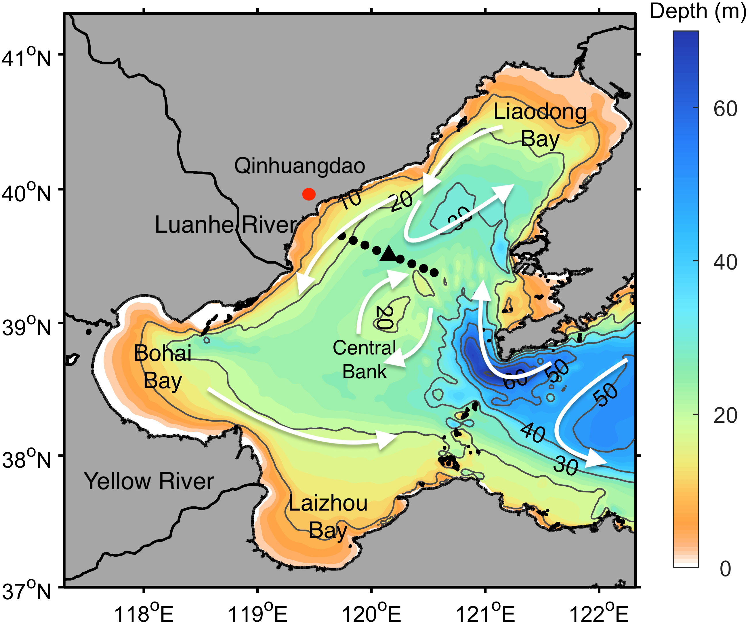
Figure 1 Bathymetry of the Bohai Sea with the sampling stations indicated. The black dots and triangles represent the transect and mooring (Stn A5) stations, respectively. White arrows are schematic circulations in the BS in summer based on the numerical results of Zhou et al. (2017).

The mooring station (Stn) A5 (with a mean water depth of 27 m) is located at the deepest region of the transect lasting 48 h from 22:00, 8 August 2018. The transect observation was carried out during 8–9 August 2018 just after finishing the mooring observation. A bottom mooring frame that carried an upward-looking acoustic Doppler current profiler (ADCP, Signature1000), a downward-looking acoustic Doppler velocimeter (ADV, Nortek), and a CTD (RBR Concerto) was equipped at Stn A5. Figure 2 shows the sketch of the observation at Stn A5. The ADCP measured vertical profiles of velocity from a height of 1.5 m to 23.5 m with a vertical resolution of 0.5 m and a temporal resolution of 1 min. The ADV measured high-frequency velocity fluctuations continuously at a rate of 32 Hz. The CTD (RBR Concerto) measured the near-bottom temperature, DO, and turbidity. Besides the mooring observations, we deployed the CTD (RBR Maestro) and a vertical microstructure profiler (VMP-200) simultaneously once an hour during daytime and once every three hours during nighttime to obtain the continuous time-depth variations of temperature, salinity, DO, chlorophyll-a, and microstructure shear (Figure 2). Information regarding the instruments used and corresponding sampling frequencies and ranges are presented in Table 1. Due to the absence of simultaneous atmospheric measurements, the sea surface temperature, net heat flux, wind speed, and significant wave height are from the ERA5 reanalysis data.

FIGURE 2

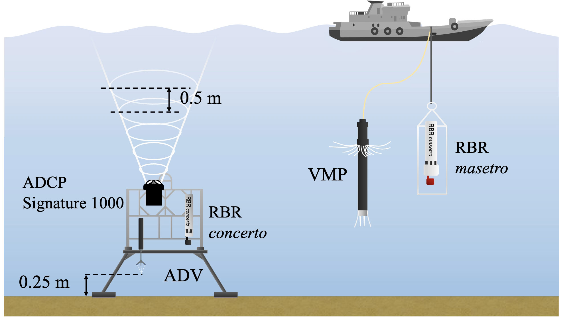
Figure 2 Sketch of the field observations.

TABLE 1

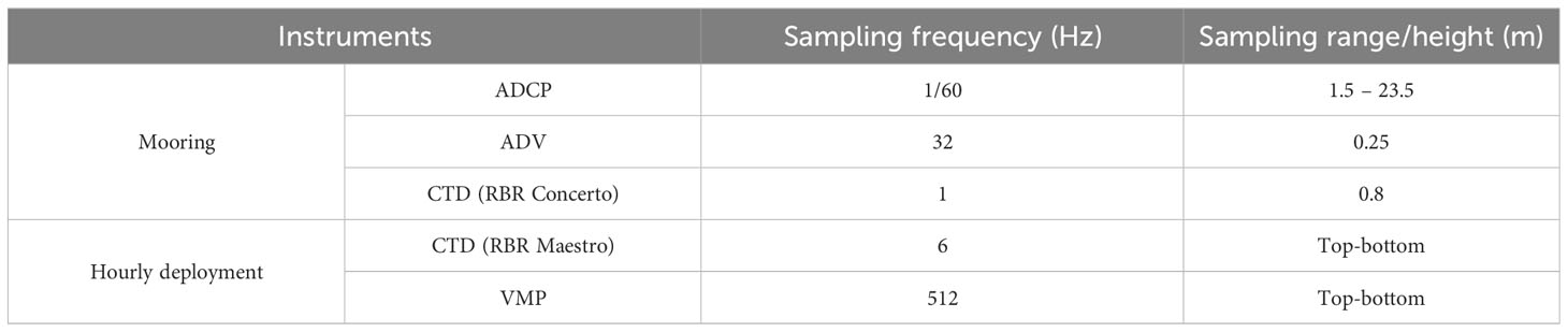
Table 1 Instrument sampling frequencies and corresponding sensor sampling ranges.

2.2 Data processing

The high-frequency velocity fluctuations measured by ADV were used to calculate the near-bottom turbulent kinetic energy dissipation rate ($ϵ$) according to the inertial dissipation method (Yang et al., 2017). In principle, the calculated vertical velocity spectra of each 1-min segment were fitted to their theoretical forms within the -5/3 inertial subrange. Based on Taylor’s frozen turbulence hypothesis, the energy spectrum can be written as

$\begin{array}{ll}{S}_{ww}(f)=\frac{\alpha \overline{U}{ϵ}^{2/3}{k}^{-5/3}}{2\pi }& \text{, (1)}\end{array}$

where $\overline{U}$ is the averaged velocity magnitude over a 1-min segment, $\alpha$ = 0.71 is the corresponding one-dimensional Kolmogorov constant, k is the wavenumber, and $S_{ww}(f)$ is the observed vertical velocity frequency spectrum. The turbulent kinetic energy dissipation rate ($ϵ$) was calculated and averaged within the subrange of 1 and 5 Hz.

Based on Prandtl’s analysis, the near-bottom velocity shear can be scaled as

$\begin{array}{ll}\frac{\partial u}{\partial z}=\frac{u_{*}}{\ell }& \text{, (2)}\end{array}$

where $\ell$ is the mixing length scale. A reasonable choice for $\ell$ near the bottom is $\ell =\kappa z$, where $\kappa$ (0.41) is the von Karman constant and z is the height above the bottom. By employing $\ell =\kappa z$, the shear production of turbulent kinetic energy (TKE) ($P=-\overline{u^{\prime }{w}^{\prime }}\frac{\partial u}{\partial z}--\overline{v^{\prime }{w}^{\prime }}\frac{\partial v}{\partial z}$) can then be simplified to $\frac{u_{*}^3}{\kappa z}$. The scaled shear production of TKE is then compared with the dissipation of turbulent kinetic energy (TKE).

The microstructure shear measured by VMP was used to calculate $ϵ$ across the water column. Under the assumption of isotropic turbulence, $ϵ$ was calculated following

$\begin{array}{ll}ϵ=7.5\nu \overline{{(\partial u/\partial z)}^2}=7.5\nu \underset{k_1}{\overset{k_2}{\int }}\varphi (k)dk& \text{, (3)}\end{array}$

where ∂u/∂z is the vertical shear of the horizontal velocity fluctuation, ν is the molecular viscosity, ϕ(k) is the power spectrum of the vertical shear, and k₁ and k₂ are the lower and upper limits of wavenumber for integration, respectively. $ϵ$ was calculated by fitting the empirical Nasmyth spectrum to the measured shear spectra over consecutive segments of 2 m with a 50% overlap. Vertical profiles of $ϵ$ with a vertical resolution of 1 m were then obtained (Xu et al., 2020a; Yang et al., 2023). The vertical eddy diffusivity ($K_{\rho }$) was calculated using the Osborn (1980) relation, $K_{\rho }=\text{Γ}\frac{ϵ}{N^2}$. The mixing efficiency (Γ) was employed to be the traditional constant value of 0.2 (Osborn, 1980).

The squared velocity shear was calculated following $S^2={(\frac{\partial u}{\partial z})}^2+{(\frac{\partial v}{\partial z})}^2$, where $u$ and $v$ are the zonal and meridional velocities, respectively. The squared buoyancy frequency was calculated according to $N^2=-\frac{g}{{\rho }_0}\frac{\partial \rho }{\partial z}$, where $g$ is the gravitational acceleration and $\rho$ is water density. The gradient Richardson number was then calculated according to Ri = $\frac{N^2}{S^2}$. The residual currents were calculated by removing tidal constituents from the raw velocity measurements. The tidal constituents were analyzed using the T_TIDE Matlab toolbox (Pawlowicz et al., 2002).

3 Results

3.1 Characteristic physical and biogeochemical features of the study area

The characteristic physical and biogeochemical features of the study area were examined based on the transect observations (Figure 3). The water column remains stratified across the transect. Despite the overall stable stratification, the stratification weakens as the bathymetry becomes shallower approaching the coast (Stns A1 and A2). The boundaries of the surface boundary layer (SBL) and bottom boundary layer (BBL) in this work are defined as the depth at which the density exceeds 0.1 kg m^-3 difference with the top and bottom density measurements, respectively. The stratified interior layer (IL) is located between the SBL and BBL. There exist apparent horizontal gradients of temperature and density in the BBL, indicating the presence of BBL fronts (Figures 3A, C). Such BBL fronts can act as horizontal barriers restricting the lateral oxygen supply which favors the maintenance of bottom oxygen depletion (Zhao et al., 2017; Zhang et al., 2022).

FIGURE 3

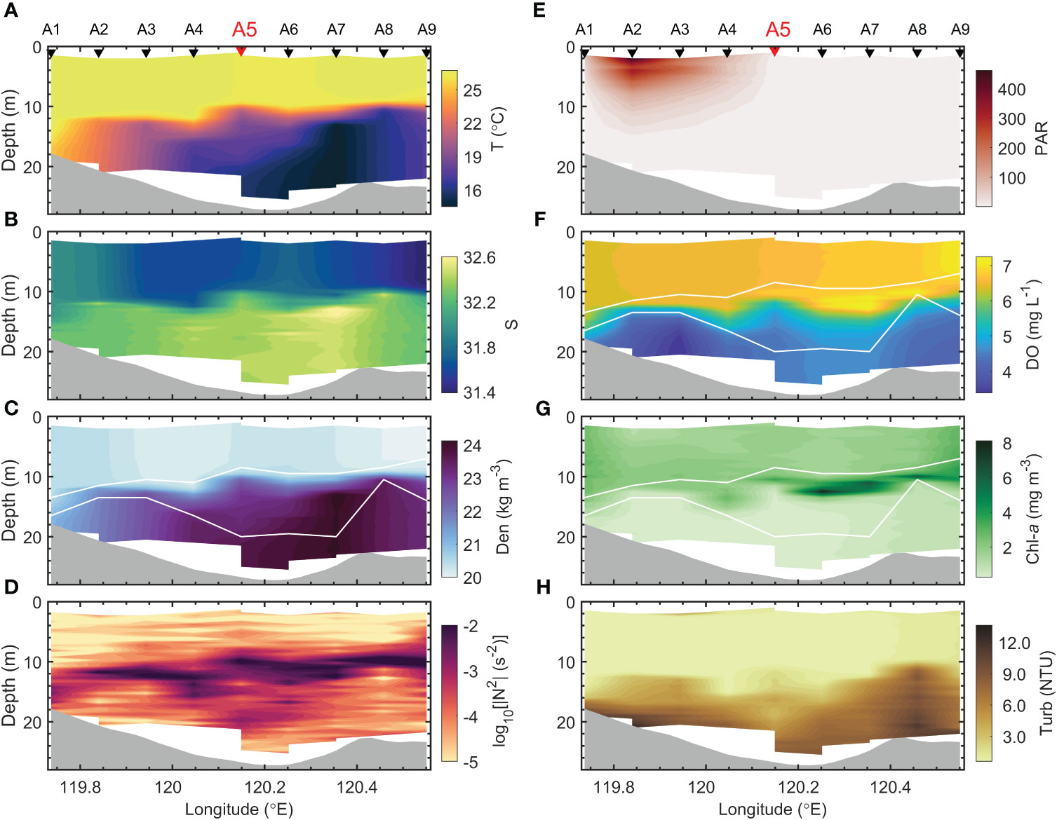
Figure 3 Spatial distribution of (A) temperature, (B) salinity, (C) density, (D) squared buoyancy frequency (N²), (E) photosynthetically active radiation (PAR), (F) dissolved oxygen (DO), (G) chlorophyll-a, and (H) turbidity. The black inverted triangles at the top represent the locations of transect stations with the station names in text nearby. The mooring station (Stn A5) is indicated with the red inverted triangle. The white contours in (C, F, G) represent the boundaries of the surface and bottom boundary layers. The white areas near the sea surface and bottom have no data due to measurement limitations.

The DO concentration shows a typical three-layer structure: the oxygenated SBL, oxygen-depleted BBL, and a transition layer between them (Figure 3F). The depth ranges of the SBL and BBL varies along the section. The SBL changes from 14 m at Stn A1 to 7 m at Stn A9. The BBL has an average thickness of ~ 8 m over the whole section. Two patchy low-DO zones are located at the west and east slopes, respectively. The lowest DO concentration appears at the west low-DO zone which is less than 4 mg L^-1. A subsurface DO maximum is found at ~ 10 m depth at Stns A6 and A7 corresponding to the high chlorophyll-a concentration there (Figure 3G). Furthermore, the transect reveals high turbidity at two low-DO zone (Figure 3H). As we will show below, the occurrence of a high-turbidity event at the mooring station can lead to severe oxygen decline. These results, therefore, coincide with each other, indicating the important role of suspended organic matter in DO consumption.

3.2 Temporal variation of hydrographic properties

The temperature and salinity at Stn A5 generally shows a three-layer structure with a warm, fresh SBL, a cold, salty BBL, and a stratified IL (Figure 4). The temperature and salinity difference between the surface and bottom layers can reach ~ 12°C, and 1, respectively. The near-surface temperature showed an increasing trend throughout the observation period (Figure 4B). This could have been induced by the warming trend of air temperature (Figure 4F). The surface warming induced a near-surface stratification in the upper ~ 8 m after 12 h (Figures 4D, E). The DO vertically changed from an oxygenated SBL to an oxygen-depleted BBL (Figure 4H). Higher subsurface DO centration occasionally occurred corresponding to the periodic occurrence of high subsurface chlorophyll-a in the IL.

FIGURE 4

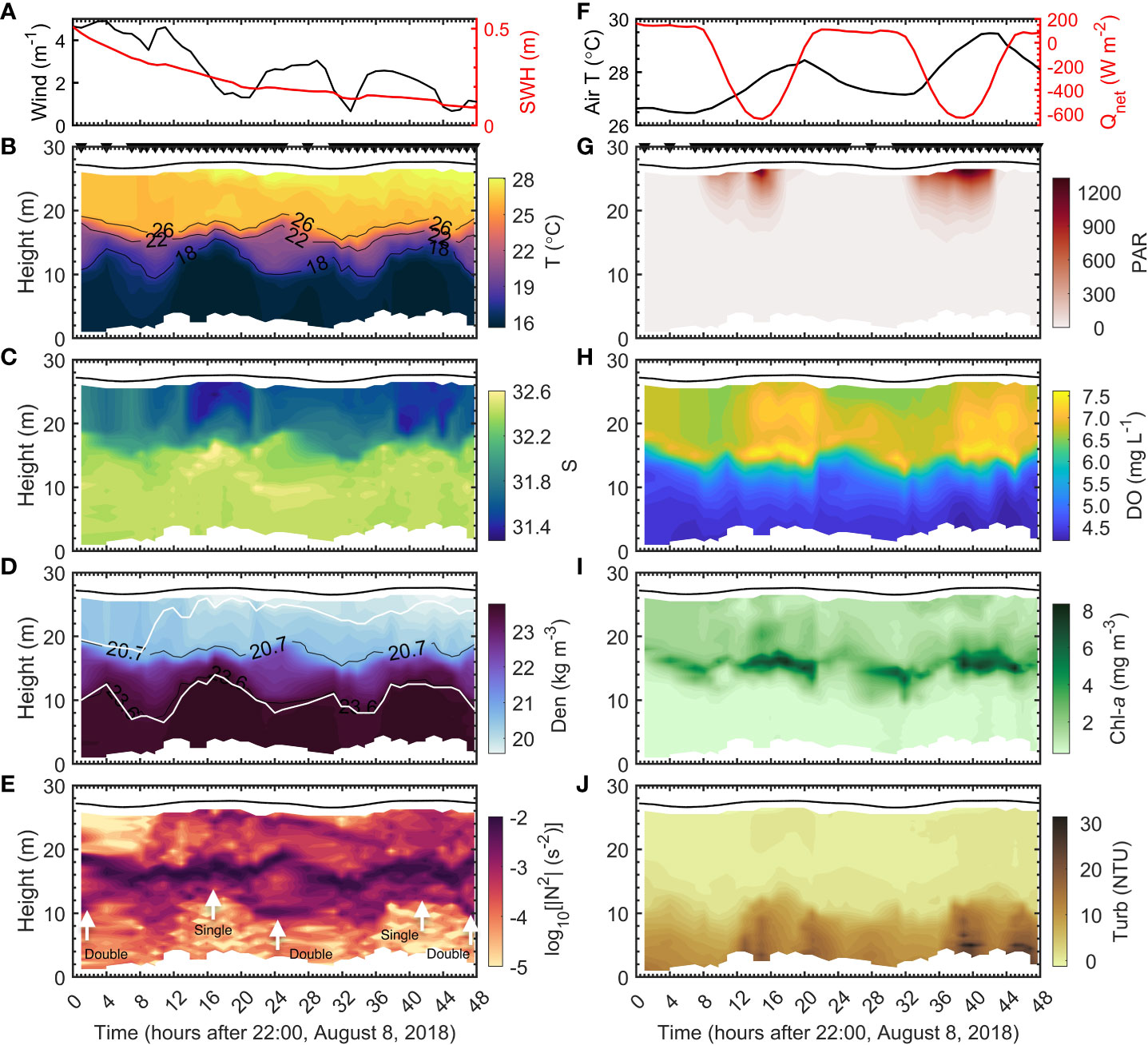
Figure 4 Temporal variations of (A) wind speed and significant wave height and (F) air temperature and net sea surface heat flux at Stn A5. Time-depth variations of (B) temperature, (C) salinity, (D) density, (E) squared buoyancy frequency (N²), (G) photosynthetically active radiation (PAR), (H) dissolved oxygen (DO), (I) chlorophyll-a, and (J) turbidity. The overlying black lines represent the time evolution of surface elevation. The black inverted triangles denote the time of deployment. The “single”, “double” and corresponding arrows in (E) denote the appearance of a single- and double-pycnocline. The white contours in (D) represent the boundaries of the surface and bottom boundary layers. The white areas near the sea surface and bottom have no data due to measurement limitations.

An interesting phenomenon observed here was that the water column showed a periodic shifting between single and double pycnocline cases (Figure 4E). Single and double pycnoclines are mainly found during the high tide and ebb phases, respectively. Figure 4D shows that the 20.7 and 23.6 kg m^-3 isopycnolines periodically move closer and further away from each other. Figures 5A, B show the representative temperature, salinity, DO, and chlorophyll-a profiles of the single- and double-pycnocline cases at 18 and 24 h, respectively. When the pycnocline was separated into two parts, the upper and lower pycnoclines were located around a height of ~18 m and ~10 m, respectively. Higher subsurface chlorophyll-a and DO concentrations appeared when there was one single pycnocline that appeared during high tides (12 – 20, 38 – 46 h).

FIGURE 5

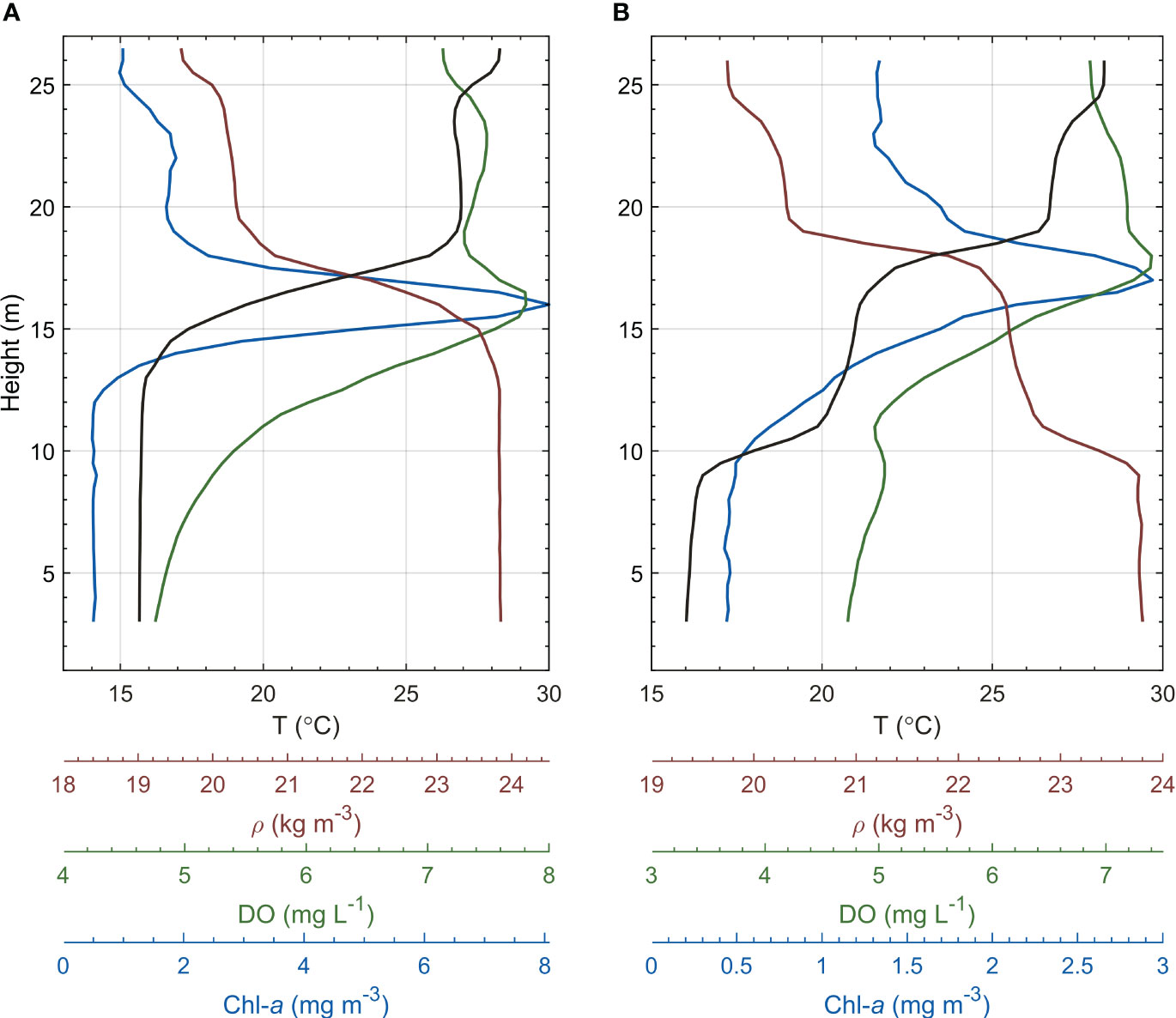
Figure 5 Vertical profiles of temperature, density, DO, and chlorophyll-a at (A) 18 h and (B) 24 h which represent typical profiles of single- and double-pycnocline cases, respectively.

The temperature and DO as measured by the moored near-bottom RBR Concerto and deepest sample of the profiling RBR Maestro are shown in Figure 6. These two measurements agreed well with each other, both showing obvious tidal variability. Tidal advection of different water masses which has apparent spatial temperature and DO gradient could induce the tidal variability of hydrographic properties at a fixed location. The tidal variability agreed with the apparent horizontal temperature and DO gradients as revealed in the transect observations (Figure 3). Although there are other factors that may also induce tidal variability, we suggest tidal horizontal advection is the dominant reason. Supporting evidence includes that the estimations of horizontal gradient based on the transect observation and the least squares method of the moored observations in temporal space show reasonable agreement with each other. This is examined in detail in Section 5.1.

FIGURE 6

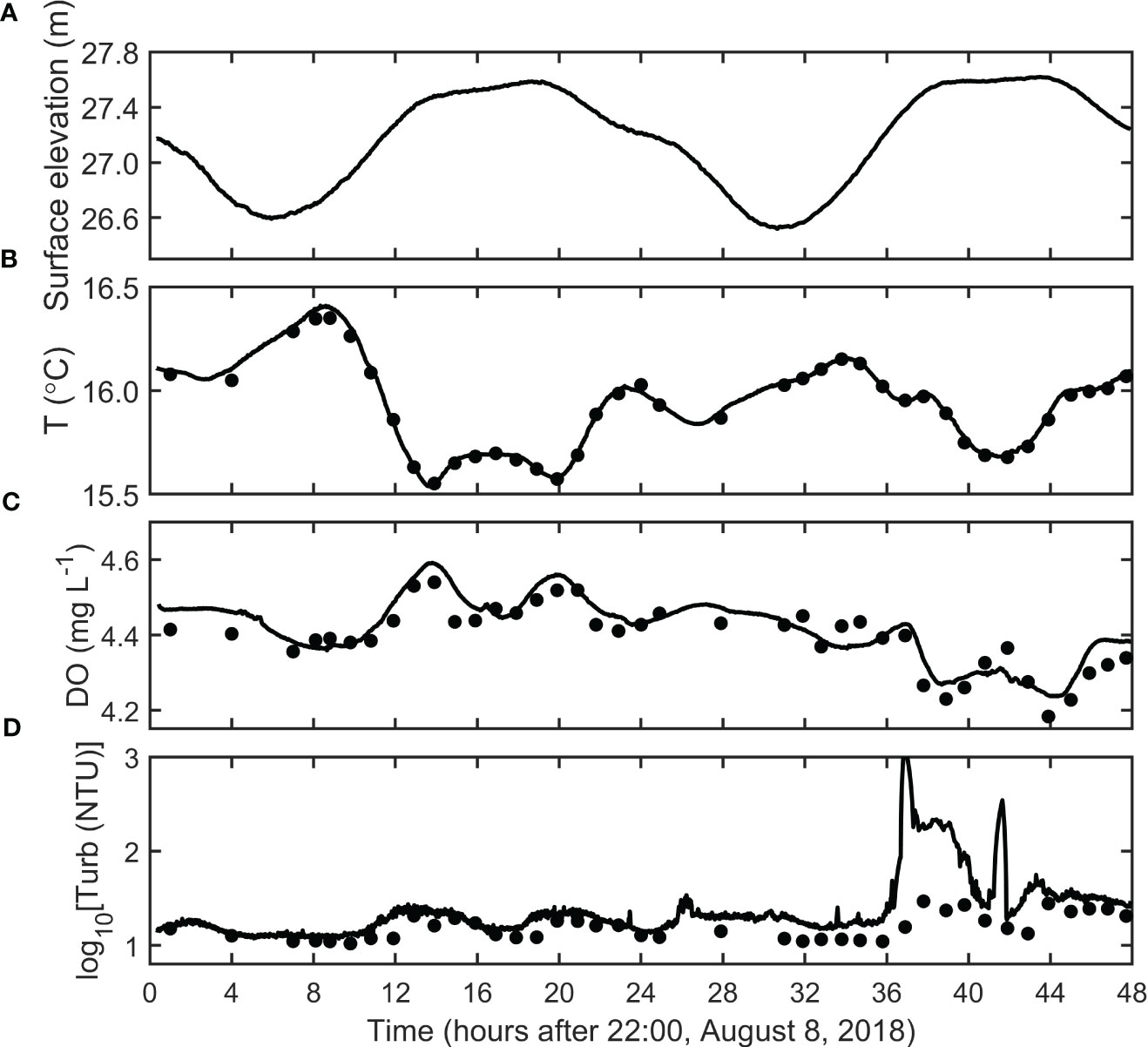
Figure 6 Time series of (A) surface elevation and near-bottom (B) temperature, (C) DO, and (D) turbidity. The black lines are measured by the RBR Concerto at 0.8 m above the bottom. The black dots in (B–D) represent the deepest sample of the profiling measurements of RBR Maestro.

The highest temperature was observed at ~ 8 and 34 h during the low tide. The near-bottom DO concentration and temperature generally showed an opposite variation trend before 37 h. The highest DO concentration was observed during high tides when the lowest temperature appeared (12 – 20 h). According to this relationship, we would expect the occurrence of another DO concentration peak during 37 – 45 h when the near-bottom temperature was low. However, we observed the lowest bottom DO concentration (~ 4.3 mg L^-1) during our observation period. This indicates that the short-term variation of DO is not only influenced by the tidal horizontal advection of different water masses, but there are also other processes influencing the evolution of DO.

Along the occurrence of low-DO, a strong high-turbidity event was observed with the near-bottom turbidity increased by one order of magnitude (Figure 6D). During that time, the profiling measurements of turbidity were lower than the moored near-bottom turbidity measurements. This may be attributed to the fact that the turbidity can be greatly enhanced when approaching the seabed. Figure 4J shows that the elevated turbidity was not restricted near the bottom, but could reach the bottom of the pycnocline. As we will show, a high-turbidity event plays an important role in inducing the low DO. The detailed bottom DO dynamics will be discussed in Section 5.

3.3 Current, shear, and turbulence properties

Figure 7A shows the barotropic tidal ellipses as measured by the bottom-moored ADCP. The barotropic flow was calculated by vertically averaging the measured velocity over the whole profile. The current rotated clockwise with the maximum barotropic velocity exceeding 0.5 m s^-1. Figure 7B shows that the reconstructed tidal ellipses resemble the current ellipses well. M₂ and K₁ represent the two most important tidal constituents with their ellipses all elongated in the direction along isobaths. The major axis of M₂ (0.36 m s^-1) is about two times larger than that of K₁ (0.19 m s^-1). This agrees with the Ocean Atlas and EOT20 model that M₂ tide is the dominant tidal constituent in the BS, having larger maximum amplitudes over that of S₂, K₁, and O₁ tides (Chen, 1992; Pan et al., 2022, their Figure 2). Figures 8A, B show that the observed velocity has little phase difference in the vertical direction. Most of the large velocity shear appeared in the pycnocline (Figure 8C). Intensified pycnocline velocity shear seemed to occur when a double pycnocline was present (0 – 4, 22 – 28, 44 – 48 h).

FIGURE 7

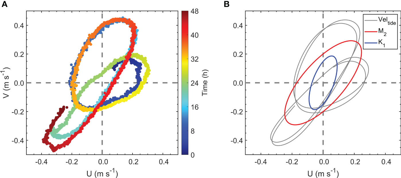
Figure 7 (A) Depth-averaged ADCP current ellipses in a 1-min interval. Colors represent the measurement time. (B) The gray line represents the reconstructed tidal current ellipses based on the harmonic analysis using the T_TIDE Matlab toolbox (Pawlowicz et al., 2002). Red and blue lines represent the M₂ and K₁ constituents, respectively.

FIGURE 8

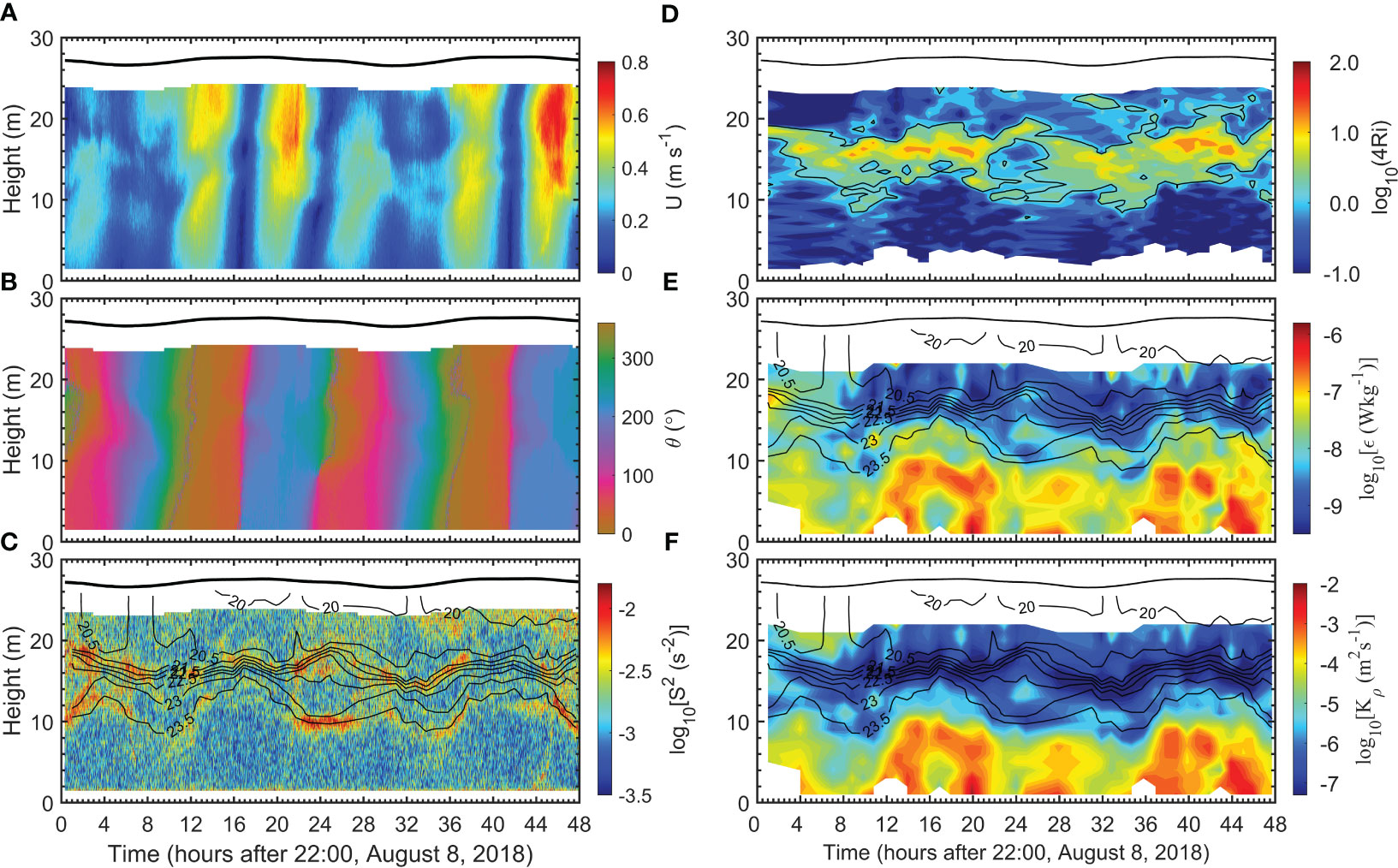
Figure 8 Time-depth variations of (A) velocity magnitude, (B) velocity direction, (C) squared velocity shear (S²), (D) Richardson number (Ri), (E) $ϵ$, and (F) $K_{\rho }$. Black contours in (D) represent Ri = 0.25. Black contours in (C, E, F) represent isopycnal lines. The overlying black lines represent the time evolution of surface elevation. The white areas near the sea surface and bottom have no data due to measurement limitations.

The measured $ϵ$ showed that the strongest turbulence ($ϵ$ > 10^-6 W kg^-1) was located in the BBL (Figure 8E). Active turbulence in the SBL was missing because we eliminated the near-surface 10 m VMP observations which were presumably contaminated by ship-induced disturbances. Furthermore, the wind speed at Stn A5 was very weak (< 4.5 m s^-1) during the observation period. The significant wave height also showed a weakening trend (Figure 4A). Dissipation in the BBL was dominated by tidally driven quarter- to semi-diurnal variability which is attributed to the tidally induced bottom friction. This agrees with the result of Xu et al. (2020b) which showed that tidal forcing can play an important role in determining the water column turbulence level in the BS. Large $ϵ$ can extend to the base of the pycnocline. The potential occurrence of shear instability can be diagnosed with the gradient Richardson number. Figure 8D shows that low Ri (Ri< 0.25) mostly occurred in the BBL corresponding to the intense turbulence there.

The near-bottom ADV measurements revealed a similar close relationship between the velocity magnitude and turbulence intensity (Figure 9). The intense dissipation could reach 5 × 10^-5 W kg^-1. Figure 9 shows that shear production of TKE P generally coincided with $ϵ$ during the observation period. This demonstrates the dominant role of shear production generated by the tidal bottom friction in inducing the near-bottom turbulence.

FIGURE 9

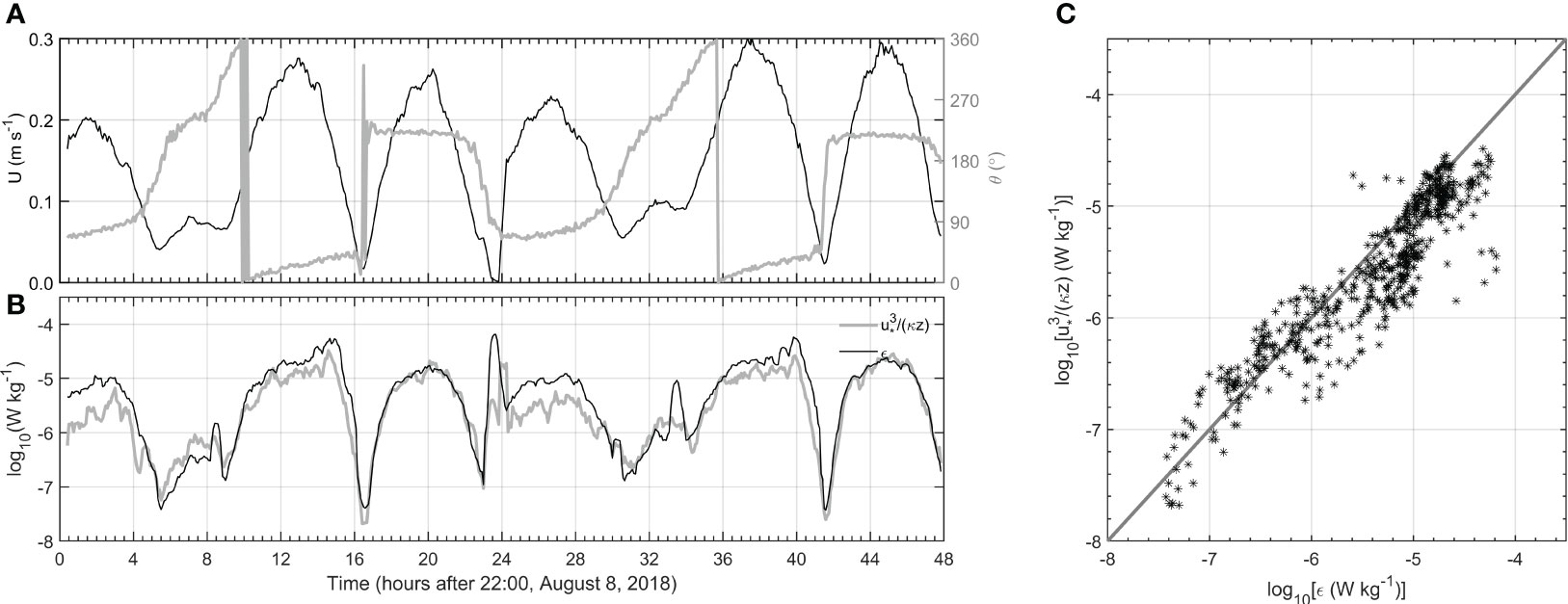
Figure 9 Time series of the near-bottom (A) velocity magnitude and direction and (B) $\epsilon$ and scaled shear production ($\frac{u_{*}^3}{\kappa z}$). (C) Observed $\epsilon$ versus the shear production based on the law of the wall. The gray line denotes P = $\epsilon$.

Turbulence within the pycnocline was weak ($ϵ$ ~ 10^-9 W kg^-1) overall due to the suppression effect of stratification. Consequently, weak mixing and low values of $K_{\rho }$ were observed within the pycnocline (Figure 8F). The pycnocline could then act as a barrier limiting the vertical DO fluxes and the replenishment of BBL oxygen. Despite the overall weak turbulence, we found occasional large $ϵ$ in the pycnocline. Stronger pycnocline turbulence ($ϵ$ ~ 10^-8 W kg^-1) was found between the upper and lower pycnoclines around a height of ~ 15 m when a double pycnocline was present. This corresponds to the observed Ri< 0.25 between the upper and lower pycnoclines which were formed due to the weak stratification there. The bottom DO budget and detailed bottom DO dynamics are discussed in detail in the next section.

4 Discussion

4.1 Role of horizontal transport to DO budget

The DO budget in the BBL has been conducted in many previous studies (Bourgault et al., 2012; Queste et al., 2016; Cui et al., 2018). Changes in the DO concentration in the BBL are dominated by physical processes (horizontal/vertical advection and vertical turbulent fluxes) and biological processes (DO consumption due to nitrification and bacterial respiration). Specifically, the biological processes include water column organic matter respiration (WR) and sediment oxygen demand (SOD).

Based on the same mooring measurements together with monthly DO measurements in the year 2017 and 2018, Song et al. (2020) diagnosed the DO budget in the BS. Song et al. (2020) showed that the average DO concentration in the bottom water linearly decreased from May to August, reaching ~ 3.2 mg L^-1 in August. The monthly DO measurements revealed a net oxygen consumption rate of 0.075 $\pm$ 0.011 mg L^-1 d^-1 in the BBL, translating into a BBL-integrated net oxygen consumption rate of 970.2 $\pm$ 141.4 mg m^-2 d^-1. The vertical turbulent diffusion flux across the pycnocline was estimated to be 6.08 ± 6.72 mg m^-2 d^-1 using the profiling measurements of $K_{\rho }$ (as measured by VMP) and DO (as measured by RBR Maestro). The concurrently determined oxygen flux at the water-sediment boundary layer (SOD) had an average value of 202.2 ± 78.1 mg m^-2 d^-1. Assuming the horizontal advection transport of DO to be zero, the WR in the BBL was then calculated to be 766.4 mg m^-2 d^-1, 79% of the net oxygen consumption in the BBL. The diagnosis of the DO budget above is based on the assumption of negligible horizontal advection transport of DO which is applicable when there are negligible horizontal DO gradients or residual currents (Rovelli et al., 2016). Here, the DO budget as diagnosed by Song et al. (2020) is revisited with the possible influence of horizontal advective DO transport tested.

Figure 6C shows that the near-bottom DO centration time series had obvious tidal variability, implying the presence of horizontal DO gradients. Figure 3 clearly shows the presence of horizontal temperature and DO gradients along the transect. The tidal variability is depicted more clearly in Figures 10C, D in that the near-bottom T and DO showed consistent evolution during the first 37 h. A periodic warm, oxygen-depleted core occurred simultaneously. This indicates the tidal horizontal advection of different water masses (Zhang et al., 2019). From a long-term view, the horizontal DO advection transport is determined by both the horizontal DO gradient and residual currents. Previous studies have shown that the study area is mainly influenced by the anti-cyclonic flow in the central BS and cyclonic circulation around the cold pools in Liaodong Bay (Zhou et al., 2017; Zhang et al., 2020, as also indicated in Figure 10A). Therefore, the situation regarding the BS here is different from some of the previous studies, for example, in the central North Sea, where both the residual current and horizontal DO gradients are small (Rovelli et al., 2016). Whether the presence of horizontal DO gradients and residual currents can contribute to the bottom DO balance was investigated next.

FIGURE 10

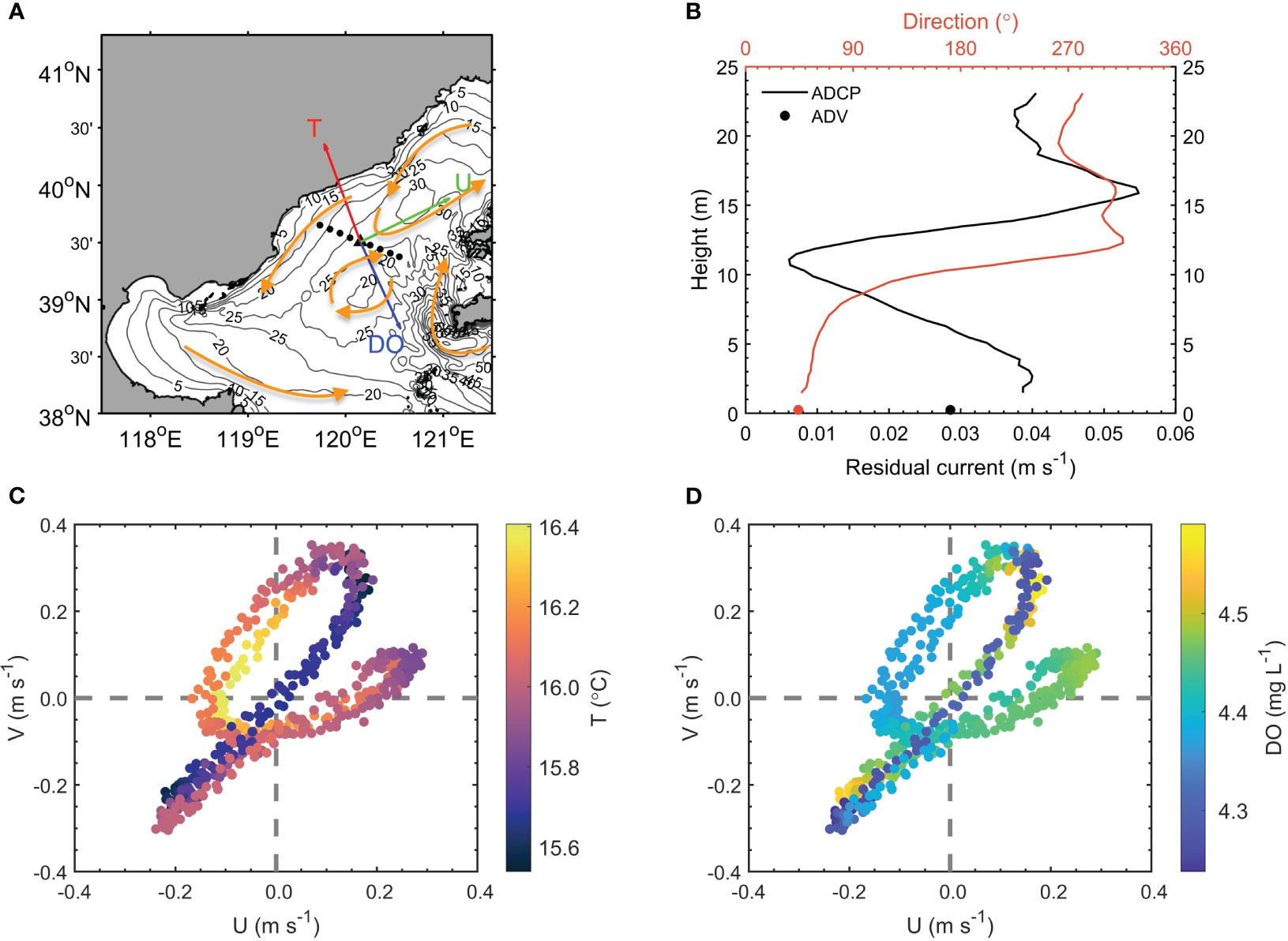
Figure 10 (A) Bathymetry (in units of m) in the BS and the location of study sites. Arrows represent the estimated directions of near-bottom horizontal gradients of temperature/DO, and the residual current. Yellow arrows are a schematic of circulations in the BS in summer based on the numerical results of Zhou et al. (2017). (B) The vertical profile of residual current magnitude and direction averaged over the observation period. Near-bottom current ellipses with the near-bottom (C) temperature, and (D) DO superimposed.

The horizontal gradient of temperature and DO was first calculated. Here the horizontal gradients are estimated based on the near-bottom temperature and DO times series and the least squares method. Assuming that the horizontal advection dominates the near-bottom hydrography transport, the temporal variation of temperature and DO follow

$\begin{array}{ll}\frac{\partial \overline{\text{ℊ}}}{\partial t}=-\overline{u}\frac{\partial \overline{\text{ℊ}}}{\partial x}-\overline{v}\frac{\partial \overline{\text{ℊ}}}{\partial y}& (4)\end{array}$

where $\overline{\text{ℊ}}$ represents the near-bottom temperature and DO; $x$ and $y$ represent the zonal and meridional directions, respectively; and $\overline{u}$ and $\overline{v}$ are the measured near-bottom zonal and meridional velocities, respectively. The mean horizontal gradient ($\frac{\partial \overline{\text{ℊ}}}{\partial x}$, $\frac{\partial \overline{\text{ℊ}}}{\partial y}$) can then be estimated using the least squares method based on Equation 2. We estimate the horizontal gradients of both temperature and DO are estimated based on measurements before 37 h. This is because that, as we will show later, the lowest DO concentration after 37 h was not driven by tidal advection. Table 2 summarizes the estimated horizontal gradients with their directions shown in Figure 10A. The horizontal DO gradient had a magnitude of 3.4 × 10^-5 mg L^-1 m^-1. The estimated near-bottom horizontal temperature and DO gradient were directed in the opposite direction which agrees with their opposite varying trends as shown in Figure 6. The horizontal gradient of T was directed to the coast, reflecting the warming of BBL T towards the coast (Figure 3A). In contrast, the horizontal gradient of DO was directed to the central bank which is associated with the low-DO zone located at the west-sloping region (Figure 3F).

TABLE 2

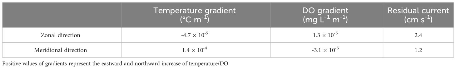
Table 2 The horizontal gradients of temperature and DO as estimated from Equation 4 and the estimated residual current.

In addition to calculating the horizontal T and DO gradient based on the near-bottom mooring measurements and the least squares method, we next calculated the horizontal DO gradient from the transect observation which allowed the examination of the gradient in the along-transect direction. The horizontal gradient at Stn A5 was calculated based on the measurements at Stns A4 and A6. The averaged values below the depth of 20 m were used which showed a decreasing and increasing trend from Stns A4 to A6 for T and DO, respectively (Figures 3A, C). The horizontal gradient of bottom T and DO in the direction from Stns A4 to A6 was then estimated to be -9.1 × 10^-5°C m^-1 and 2.2 × 10^-5 mg L^-1 m^-1, respectively. The projection of the T and DO gradients estimated from Equation 4 in the along-transect direction was -9.9 × 10^-5°C m^-1 and 2.4 × 10^-5 mg L^-1 m^-1, respectively. Therefore, the two independent estimations of horizontal gradient showed good agreement with each other with a deviation of less than 10%. This demonstrates our previous conjecture that the tidal variation of near-bottom hydrography is induced by the tidal horizontal advection of different water masses. Note that given the uncertainties involved in the calculation, one should not expect a perfect match of horizontal gradients between the above two methods. For example, the relatively long distances between transect stations and the tidal variability at transect stations (which is ignored here) can both induce uncertainties. Nevertheless, the reasonable agreement between the two methods suggests that the short-term variations of T and DO are essentially driven by the tidal horizontal advection. We speculate that the residual horizontal advection of DO may also play a role in the bottom DO balance here.

The residual current was calculated as the difference between the original current and the tidal current. The tidal current was extracted using the harmonic analysis (T_tide package). Although the residual currents in the upper layer were variable, they showed a constant northeastward direction in the BBL (figure omitted). The vertical profile of the time-averaged residual currents showed that the residual current in the BBL directs northeastward (Figure 10B). The averaged residual current was 2.7 cm s^-1 in the BBL directing northeastward (63° with 0° directing northward). This coincides with the previously concluded anti-cyclonic flow in the central BS which can in turn induce the northeastward residual current at the study site (Zhou et al., 2017).

Assuming that the horizontal DO gradient is constant in the BBL, the horizontal advection of DO to our study site was calculated using the values of the measured residual current and horizontal DO gradient. The horizontal advection of DO integrated over the BBL (13 m, to keep consistency with Song et al., 2020) had a value of 67.4 mg m^-2 d^-1. Here, a positive value represents that currents transport relatively high-oxygen water to the study site. The magnitude of horizontal DO transport was about 33% of the SOD, but was about one order over the oxygen supply via vertical turbulent flux. After considering the horizontal and vertical supply of DO in the bottom DO budget, the WR in the BBL was then calculated to be the residual reaching 841.5 mg m^-2 d^-1. The estimation of WR here was ~ 75 mg m^-2 d^-1 larger than that of Song et al. (2020), which neglected the horizontal advection and vertical diffusion supply of DO.

Based on a coupled physical-biogeochemical model, Zhang et al. (2022) showed that while the net effects of oxygen advection in the BS are negligible, the spatial distribution of DO is significantly influenced by the DO advection. The relatively low-oxygen waters off QHD are transported northward. Our results, therefore, agree with the numerical results demonstrating the role of horizontal DO advection in modulating DO depletion. While we have shown that the horizontal advection effect contributes to the BBL DO budget here, the DO advection may play a less important role than those near estuaries. For example, based on observations in the Pearl River Estuary and adjacent shelf sea, Cui et al. (2018) showed that the DO advection by gravitational circulation from DO-rich shelf benthic waters is roughly balanced by the bacterial respiration in the water column.

The main reason leading to the less important role of advection at our study site is that the directions of the residual current and horizontal DO gradient are nearly perpendicular (~ 94°) to each other. The reasons for the perpendicular direction are an interesting topic. The residual currents (circulation) in the summer BS are in geostrophic balance which mainly flows along the isopycnal lines/bottom front (Xu et al., 2023). Meanwhile, the isopycnal lines/bottom front can act as the horizontal barrier of DO; therefore, the horizontal DO gradient usually exists in the cross-front direction. This case in a shelf sea is quite different from that in a river estuary where the gravitational circulation (not in geostrophic balance) has the same direction as the horizontal DO gradient. However, as we have shown, despite the less important role of horizontal DO advection, it can still play an important role in modulating the DO variation, which agrees with the result of Zhang et al. (2022). The role of horizontal advection on the bottom DO budget over the whole BS awaits further exploration based on more observations at different sites.

4.2 High-turbidity event and its influences on bottom DO

As discussed above, the near-bottom DO showed distinct variations before and after 37 h. Warm and oxygen-depleted water occurred simultaneously which was induced by the tidal horizontal advection of different water masses as discussed above (Figure 6C). This induced a negative correlation between the near-bottom temperature and DO before 37 h. The negative correlation between temperature and DO is depicted more clearly in Figure 11. The DO showed a negative correlation with temperature before 37 h. The best linear fitting between DO and temperature followed DO = -0.21T + 7.83 using the data before 37 h (gray line in Figure 11). However, the DO concentration during 37 – 45 h deviated from the linear fitting line.

FIGURE 11

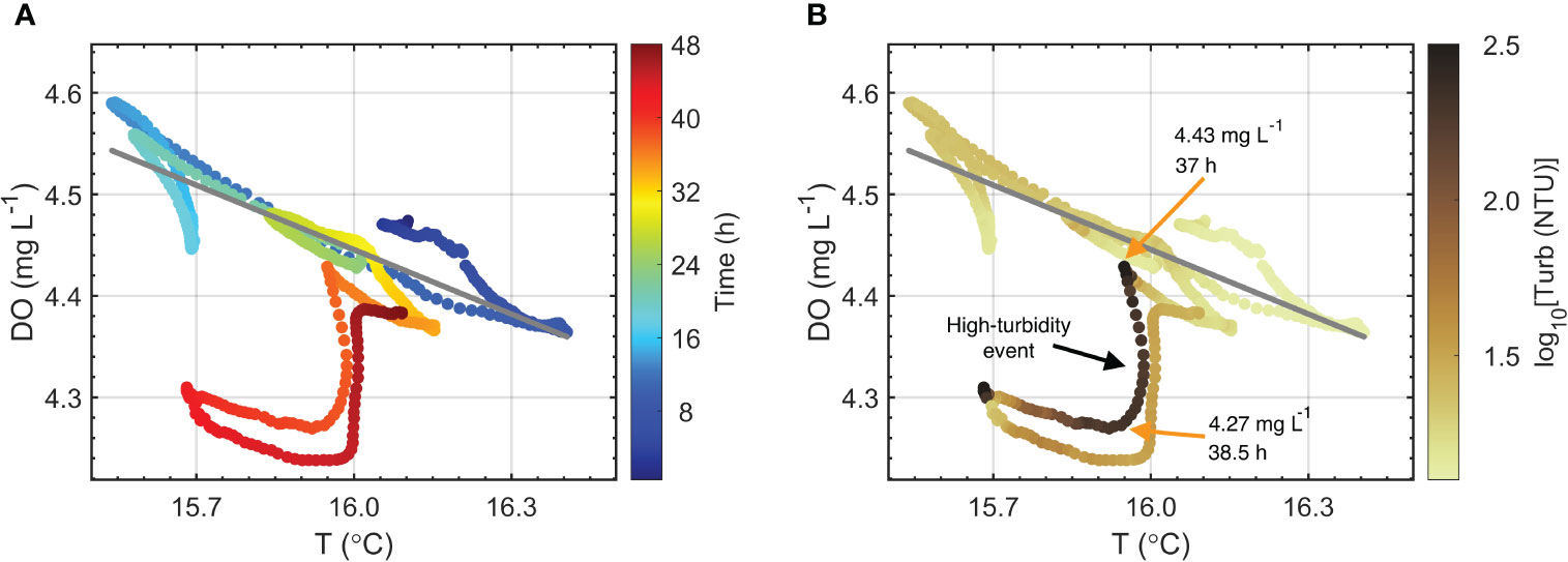
Figure 11 Temperature-DO diagram with the (A) measurement time and (B) turbidity superimposed. The gray line represents the best linear fitting between temperature and DO based on the measurements before 37 (h). The two yellow arrows marked the start and the end of the DO sudden drawdown as induced by the high-turbidity event. The corresponding measurement time and DO concentration are shown nearby.

To depict this more clearly, the temporal variation of DO was next reconstructed based on two methods. Based on the observed linear relationship between DO and temperature, the near-bottom DO concentration after 37 h was first constructed using the linear relationship between DO and temperature before 37 h. Second, the near-bottom DO after 37 h was constructed based on the concept of the tidal advection of water masses. The horizontal DO gradient estimated in section 5.1 (Table 2) and the observed near-bottom velocity were first used to estimate the temporal gradient of DO. The time series of DO concentration was then estimated by integrating the DO gradient over time. Figure 12B shows that these two approaches all predict a DO concentration peak during 38 – 44 h, which is in contrast to the observed DO minimum. The associated driving mechanism of the unexpected lowest DO concentration was investigated next.

FIGURE 12

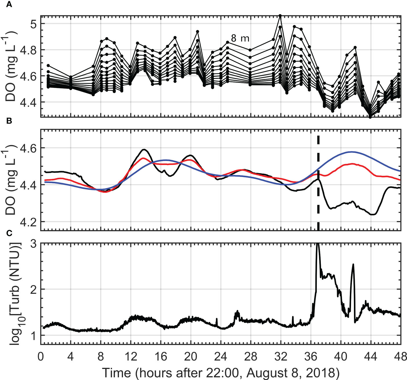
Figure 12 Time series of (A) DO in the BBL and near-bottom (B) DO and (C) turbidity. The dotted lines in (A) are separated from each other by 0.5 m with the uppermost one representing observations at a height of 8 m. The red and blue lines in (B) represent the reconstructed DO based on the best fitted linear relation with temperature and tidal advection effects, respectively. The vertical dashed line in (B) corresponds to 37 h when the measured and reconstructed DO start to deviate from each other.

The occurrence of DO minimum suggests the presence of factors other than the tidal horizontal advection influence the DO variation. Along with the occurrence of the low-DO event, we observed high near-bottom turbidity which was elevated by over one order of magnitude, reaching 260 nephelometric turbidity units (NTU) (Figure 12). Figure 11B reveals this more clearly, in that the abrupt drawdown of DO occurred simultaneously with the high turbidity. This indicates the role of the high-turbidity event in inducing the low-DO level. As discussed above, the DO consumption is mainly due to the water column organic matter respiration and sediment oxygen demand. A more rapid DO consumption during that period could have led to the observed decrease in DO concentration. In the ocean, sediment respiration is largely limited by the bioavailable surface area at the water-sediment interface. However, the bioavailable surface area can be greatly increased with the labile benthic organic matter resuspended into the water column which is available for oxidation (Greenwood et al., 2010; Queste et al., 2016). Furthermore, resuspension can also increase the exposure of anoxic, ammonium-rich sediment to oxic ammonium-poor bottom waters, thus stimulating seabed oxygen consumption via nitrification during erosional periods (Moriarty et al., 2017; Moriarty et al., 2018). These processes can then lead to the rapid oxygen consumption. Based on observations at Oyster Grounds in the North Sea, Greenwood et al. (2010) observed a strong resuspension event that led to a decrease in DO. The presented results, therefore, agree with the studies in the North Sea that the resuspension of benthic organic matter into the water column induces oxygen consumption (Greenwood et al., 2010; Queste et al., 2016).

We next sought to quantify the oxygen consumption by the high-turbidity event. Figure 11B shows that the DO dropped from 4.43 to 4.27 mg L^-1 within 1.5 h. After that, the DO reached another balanced state. We suggest that the sudden drop of DO concentration over 1.5 h was due to the rapid oxygen consumption by the high-turbidity event. Figure 12A shows that the drop of DO not only occurred near the bottom but also across the BBL. Assuming the same DO consumption rate within the BBL, the associated DO consumption rate integrated within the BBL was then estimated to be ~ 33.3 g m^-2 d^-1 (1.39 g m^-2 h^-1). This is over two orders of magnitude larger than the averaged SOD at the study site (202.2 ± 78.1 mg m^-2 d^-1) which demonstrates the important role of sediment resuspension on the BBL DO variation. This coincides with the results of the transect observations as presented above that there is high turbidity at the two low-DO zones (Figures 3F, H). The estimated increase in DO consumption rate is larger than the results of previous numerical studies. For example, based on a coupled hydrodynamic-sediment transport-biogeochemical model, Moriarty et al. (2017) showed that the modeled rates of oxygen consumption increased by factors of up to ~ 2 and ~ 8 in the seabed and below the pycnocline, respectively. The rates of oxygen consumption may depend on the amount of labile organic matter and anaerobic metabolites resuspended into the water column.

A high-turbidity event can be induced by the local sediment resuspension or advection of a non-local resuspended high-turbidity water. The simultaneous near-bottom turbulence measurements allowed us to examine the possibility of strong turbulence leading to the suspension of seafloor sediments. However, the near-bottom $ϵ$ showed regular tidal variation during the observation period which did not show abrupt intensification when high turbidity occurred (Figure 9). Natural storm events, internal waves, or human activities such as trawling can all induce the resuspension of organic material (Greenwood et al., 2010; Bianucci et al., 2018; Wang et al., 2022). The trawling intensity and distribution are patchy in the BS (Chen et al., 2022). Our study area can be subject to trawling activities which can induce severe disturbances on bottom sediment. Once the sediment is suspended, the high-turbidity water can then be advected to the study site by tidal flow.

Based on the available observations, we cannot answer the exact driving mechanism of the high-turbidity event. Regardless of the cause, we observed that high turbidity can lead to intense oxygen consumption of over two orders of magnitude larger than the SOD, resulting in the short-lived drawdown of near-bottom DO. To the best of our knowledge, no published study has investigated the effect of resuspension on oxygen depletion in the BS. The contribution of the sediment resuspension to the DO evolution over the BS depends on both the occurrence frequency and intensity of resuspension events. More observations are needed to evaluate the ecological consequence of sediment resuspension. Nevertheless, the role of sediment resuspension in controlling the near-bottom DO evolution is highlighted in this study. The presented results, therefore, also highlight the importance of the coupled physical-biogeochemical model to include the sediment resuspension effect to improve the accuracy of DO predictions.

5 Conclusions

Based on summertime mooring and transect observations off Qinhuangdao City in the BS, the properties of hydrography, turbulence, and BBL DO dynamics were studied. The study area is characterized by strong tidal forcing and obvious horizontal temperature and DO gradients in the BBL. The strongest turbulence was observed in the BBL which was induced by the bottom friction of tidal currents. The near-bottom ADV measurements showed that the largest $ϵ$ reached ~ 5 × 10^-5 W kg^-1 which could be well parameterized by the law of the wall, demonstrating the dominant role of local shear production. The near-bottom temperature and DO showed strong tidal variability. The agreement between the horizontal temperature and DO gradients estimated based on two independent methods indicated the dominant role of tidal advection of different water masses in inducing the tidal variability. Based on the least squares method, the horizontal DO gradient was estimated to be 3.4 × 10^-5 mg L^-1 directed towards the central bank. The residual current directs northeastward which is nearly perpendicular (94°) to the DO gradient. However, the calculated horizontal DO transport in the BBL reached 67.4 mg m^-2 d^-1which is about 33% of the SOD. This indicates the non-negligible role of the horizontal DO transport to the DO budget.

An interesting phenomenon observed here was the occurrence of an abnormal low-DO event after 37 h. The near-bottom DO showed a severe drawdown of 0.16 mg L^-1 in 1.5 hours. The low-DO event was different from that induced by the tidal advection effect which in contrast predicts the occurrence of a DO peak. The occurrence of low DO was next found to be induced by the occurrence of a near-bottom high-turbidity event. Resuspended benthic organic matter can greatly increase the bioavailable surface area in bottom water and seabed, which can result in much more rapid DO consumption. The DO consumption rate induced by the high-turbidity event was estimated to be ~33.3 g m^-2 d^-1 (1.39 g m^-2 h^-1) which is two orders of magnitude larger than the SOD. Although the driving mechanism of the high turbidity remains unknown, its great influence on the bottom DO variation is demonstrated clearly. The overall contribution of the sediment resuspension to the DO evolution over the BS depends on both the occurrence frequency and intensity of resuspension events which can be influenced by tidal speeds, natural storms, and trawling activities. This highlights the importance of understanding and quantifying the impact of resuspension events on the bottom DO consumption. The presented results highlight the importance of the coupled physical-biogeochemical model to include such processes in order to improve accuracy in simulating shelf sea DO depletion. An observational network simultaneously monitoring the essential physical and biogeochemical variables would also facilitate the understanding of DO depletion.

Data availability statement

The raw data supporting the conclusions of this article will be made available by the authors, without undue reservation.

Author contributions

JZ processed data, created the figures, and completed the first draft. LZ guided data analysis and the structure of the manuscript. WY, GS, and HZ provided suggestions on the manuscript. All authors contributed to the article and approved the submitted version.

Funding

The authors declare financial support was received for the research, authorship, and/or publication of this article. This work was supported by the National Natural Science Foundation of China (grant numbers 42006018, 42276009, and 42076033) and the Tianjin Natural Science Foundation (grant numbers 21JCYBJC00500 and 21JCQNJC00590).

Acknowledgments

The authors are grateful to the scientists who participated in the data collection. The colormaps used in Figures 3, 4, 8, 10, and 11 were obtained from the cmocean package (Thyng et al., 2016).

Conflict of interest

The authors declare that the research was conducted in the absence of any commercial or financial relationships that could be construed as a potential conflict of interest.

Publisher’s note

All claims expressed in this article are solely those of the authors and do not necessarily represent those of their affiliated organizations, or those of the publisher, the editors and the reviewers. Any product that may be evaluated in this article, or claim that may be made by its manufacturer, is not guaranteed or endorsed by the publisher.

References

Bianucci L., Balaguru K., Smith R. W., Leung L. R., Moriarty J. M. (2018). Contribution of hurricane-induced sediment resuspension to coastal oxygen dynamics. Sci. Rep. 8, 15740. doi: 10.1038/s41598-018-33640-3

PubMed Abstract | CrossRef Full Text | Google Scholar

Bourgault D., Cyr F., Galbraith P. S., Pelletier E. (2012). Relative importance of pelagic and sediment respiration in causing hypoxia in a deep estuary. J. Geophys. Res. 117. doi: 10.1029/2012JC007902

CrossRef Full Text | Google Scholar

Chen D. (1992). Marine Atlas in the Bohai Sea, Yellow Sea and the East China Sea (Beijing (in Chinese: Ocean Press).

Google Scholar

Chen Z., Jiang W., Lu Y., Mao X., Liu X., Wang T. (2022). Impacts of instrumented bottom frame on flow and turbulence measurements. J. Atmos. Ocean. Tech. 39 (10), 1445–1456. doi: 10.1175/JTECH-D-21-0148.1

CrossRef Full Text | Google Scholar

Chi L., Song X., Yuan Y., Wang W., Cao X., Wu Z., et al. (2020). Main factors dominating the development, formation and dissipation of hypoxia off the changjiang estuary (CE) and its adjacent waters, China. Environ. pollut. 265, 115066. doi: 10.1016/j.envpol.2020.115066

PubMed Abstract | CrossRef Full Text | Google Scholar

Cui Y. S., Wu J. X., Ren J., Xu J. (2018). Physical dynamics structures and oxygen budget of summer hypoxia in the Pearl river estuary. Limnol. Oceanogr. 64, 131–148. doi: 10.1002/lno.11025

CrossRef Full Text | Google Scholar

Diaz R. J. (2001). Overview of hypoxia around the world. J. Environ. Qual. 30, 275–281. doi: 10.2134/jeq2001.302275x

PubMed Abstract | CrossRef Full Text | Google Scholar

Diaz R. J., Rosenberg R. (2008). Spreading dead zones and consequences for marine ecosystems. Science 321, 926–929. doi: 10.1126/science.1156401

PubMed Abstract | CrossRef Full Text | Google Scholar

Fennel K., Testa J. M. (2019). Biogeochemical controls on coastal hypoxia. Ann. Rev. Mar. Sci. 11, 4.1–4.26. doi: 10.1146/annurev-marine-010318-095138

CrossRef Full Text | Google Scholar

Greenwood N., Parker E. R., Fernand L., Sivyer D. B., Weston K., Painting S. J., et al. (2010). Detection of low bottom water oxygen concentrations in the North Sea; implications for monitoring and assessment of ecosystem health. Biogeosciences 7, 1357–1373. doi: 10.5194/bg-7-1357-2010

CrossRef Full Text | Google Scholar

Moriarty J. M., Harris C. K., Fennel K., Friedrichs M. A. M., Xu K., Rabouille C. (2017). The roles of resuspension, diffusion and biogeochemical processes on oxygen dynamics offshore of the Rhône River, France: A numerical modeling study. Biogeosciences 14 (7), 1919–1946. doi: 10.5194/bg-14-1919-2017

CrossRef Full Text | Google Scholar

Moriarty J. M., Harris C. K., Friedrichs M. A. M., Fennel K., Xu K. (2018). Impact of seabed resuspension on oxygen and nitrogen dynamics in the northern Gulf of Mexico: A numerical modeling study. J. Geophys. Res. Oceans 123, 7237–7263. doi: 10.1029/2018JC013950

CrossRef Full Text | Google Scholar

Osborn T. R. (1980). Estimates of the Local rate of vertical diffusion from dissipation measurements. J. Geophys. Res. OceansJ. Phys. Oceanogr 10 (1), 83–89. doi: 10.1175/1520-0485(1980)010<0083:EOTLRO>2.0.CO;2

CrossRef Full Text | Google Scholar

Pan H. D., Jiao S. Y., Xu T. F., Lv X. Q., Wei Z. X. (2022). Investigation of tidal evolution in the Bohai Sea using the combination of satellite altimeter records and numerical models. Estuar. Coast. Shelf S. 279, 108140. doi: 10.1016/j.ecss.2022.108140

CrossRef Full Text | Google Scholar

Pawlowicz R., Beardsley B., Lentz S. (2002). Classical tidal harmonic analysis including error estimates in MATLAB using T_TIDE. Comput. Geosciences 28 (8), 929–937. doi: 10.1016/S0098-3004(02)00013-4

CrossRef Full Text | Google Scholar

Queste B. Y., Fernand L., Jickells T. D., Heywood K. J., Hind A. J. (2016). Drivers of summer oxygen depletion in the central North Sea. Biogeosciences 13 (4), 1209–1222. doi: 10.5194/bg-13-1209-2016

CrossRef Full Text | Google Scholar

Rabouille C., Conley D. J., Dai M. H., Cai W. J., Chen C. T. A., Lansard B., et al. (2008). Comparison of hypoxia among four river dominated ocean margins: The Changjiang (Yangtze), Mississippi, Pearl, and Rhône rivers. Cont. Shelf Res. 28, 1527–1537. doi: 10.1016/j.csr.2008.01.020

CrossRef Full Text | Google Scholar

Rovelli L., Dengler M., Schmidt M., Sommer S., Linke P., McGinnis D. F. (2016). Thermocline mixing and vertical oxygen fluxes in the stratified Central North Sea. Biogeosciences 13 (5), 1609. doi: 10.5194/bg-13-1609-2016

CrossRef Full Text | Google Scholar

Song N. Q., Wang N., Lu Y., Zhang J. R. (2016). Temporal and spatial characteristics of harmful algal blooms in the Bohai Sea during 1952–2014. Cont. Shelf Res. 122, 77–84. doi: 10.1016/j.csr.2016.04.006

CrossRef Full Text | Google Scholar

Song G., Zhao L., Chai F., Liu F., Li M., Xie H. (2020). Summertime oxygen depletion and acidification in Bohai Sea, China. Front. Mar. Sci. 7. doi: 10.3389/fmars.2020.00252

CrossRef Full Text | Google Scholar

Thyng K. M., Greene C. A., Hetland R. D., Zimmerle H. M., DiMarco S. F. (2016). True colors of oceanography: Guidelines for effective and accurate colormap selection. Oceanography 29 (3), 9–13. doi: 10.5670/oceanog.2016.66

CrossRef Full Text | Google Scholar

Wang H. N., Jia Y. G., Ji C. S., Jiang W. S., Bian C. W. (2022). Internal tide-induced turbulent mixing and suspended sediment transport at the bottom boundary layer of the South China Sea slope. J. Marine. Syst. 230, 103723. doi: 10.1016/j.jmarsys.2022.103723

CrossRef Full Text | Google Scholar

Wei Q., Wang B., Yao Q., Xue L., Sun J., Xin M., et al. (2019). Spatiotemporal variations in the summer hypoxia in the Bohai Sea (China) and controlling mechanisms. Mar. pollut. Bull. 138, 125–134. doi: 10.1016/j

PubMed Abstract | CrossRef Full Text | Google Scholar

Wei H., Zhao L., Zhang H., Lu Y., Song G. (2021). Summer hypoxia in Bohai Sea caused by changes in phytoplankton community. Anthropocene Coasts 4 (1), 77–86. doi: 10.1139/anc-2020-0017

CrossRef Full Text | Google Scholar

Williams C. A. J., Davis C. E., Palmer M. R., Sharples J., Mahaffey C. (2022). The three Rs: Resolving respiration robotically in shelf seas. Geophys. Res. Lett. 49, e2021GL096921. doi: 10.1029/2021GL096921

CrossRef Full Text | Google Scholar

Wollast R. (1998). “Evaluation and comparison of the global carbon cycle in the coastal zone and in the open ocean,” in The Sea, vol. 10 . Eds. Brink K. H., Robinson A. R. (New York: John Wiley and Sons), 213–252.

Google Scholar

Xu P. Z., Yang W., Zhao L., Wei H., Nie H. (2020b). Observations of turbulent mixing in the Bohai Sea during weakly stratified period. Haiyang Xuebao 42 (3), 1–9. doi: 10.3969/j.issn.0253–4193.2020.03.001

CrossRef Full Text | Google Scholar

Xu P. Z., Yang W., Zhu B. S., Wei H., Zhao L., Nie H. T. (2020a). Turbulent mixing and vertical nitrate flux induced by the semidiurnal internal tides in the southern Yellow Sea. Cont. Shelf Res. 208, 104240. doi: 10.1016/j.csr.2020.104240

CrossRef Full Text | Google Scholar

Xu Y., Zhou F., Meng Q., Zeng D., Yan T., Zhang W. (2023). How do topography and thermal front influence the water transport from the northern Laotieshan channel to the Bohai sea interior in summer? Deep-Sea Res. PT II 208, 105261. doi: 10.1016/j.dsr2.2023.105261

CrossRef Full Text | Google Scholar

Yang W., Wei H., Liu Z., Zhao L. (2023). Widespread intensified pycnocline turbulence in the summer stratified Yellow Sea. J. Geophys. Res. Oceans 128, e2022JC019023. doi: 10.1029/2022JC019023

CrossRef Full Text | Google Scholar

Yang W., Wei H., Zhao L. (2017). Observations of tidal straining within two different ocean environments in the East China Sea: Stratification and near-bottom turbulence. J. Geophys. Res. Oceans 122. doi: 10.1002/2017JC012924

CrossRef Full Text | Google Scholar

Zhai W., Zhao H., Su J., Liu P., Li Y., Zheng N. (2019). Emergence of summertime hypoxia and concurrent carbonate mineral suppression in the central Bohai Sea, China. J. Geophys. Res. Biogeosci. 124. doi: 10.1029/2019JG005120

CrossRef Full Text | Google Scholar

Zhang G., Wei H., Xiao J., Zhang H., Li Z. (2020). Variation of tidal front position in Liaodong Bay during summer 2017. Oceanologica Et Limnologia Sin. 51 (1), 1–12. doi: 10.11693/hyhz20190600110

CrossRef Full Text | Google Scholar

Zhang H., Wei H., Zhao L., Zhao H., Guo S., Zheng N. (2022). Seasonal evolution and controlling factors of bottom oxygen depletion in the bohai sea. Mar. pollut. Bull. 117 (113199), 1–11. doi: 10.1016/j.marpolbul.2021.113199

CrossRef Full Text | Google Scholar

Zhang W., Wu H., Hetland R. D., Zhu Z. (2019). On mechanisms controlling the seasonal hypoxia hot spots off the Changjiang River Estuary. J. Geophys. Res. Oceans 124. doi: 10.1029/2019JC015322

CrossRef Full Text | Google Scholar

Zhao H. D., Kao S. J., Zhai W. D., Zang K., Zheng N., Xu X., et al. (2017). Effects of stratification organic matter remineralization and bathymetry on summertime oxygen distribution in the Bohai Sea. China. Cont. Shelf Res. 134, 15–25. doi: 10.1016/j.csr.2016.12.004

CrossRef Full Text | Google Scholar

Zhou F., Huang D. J., Xue H. J., Xuan J. L., Yan T., Ni X. B., et al. (2017). Circulation associated with cold pools in the Bohai Sea on the Chinese continental shelf. Cont. Shelf Res. 137, 25–38. doi: 10.1016/j.csr.2017.02.005

CrossRef Full Text | Google Scholar