Abstract
Because of its special location and structure, the Western Pacific Subtropical High (WPSH) influences greatly the climate and weather in East Asia, especially the summer precipitation. To clarify how the interannual variability (IAV) of the WPSH is related to anomalies in the tropical sea surface temperature (SST) and atmospheric circulation, time series of the intensity index of the WPSH are subjected to wavelet analysis, showing IAV in the index. Characteristic indexes are defined for three key sea areas and the equatorial-latitude westerly region. After a continuous wavelet transform, the oscillation period of them is similar to that of the WPSH. The cross-wavelet transform of the four regional and two WPSH indexes is used to obtain the corresponding time-delay correlation. Regarding the potential correlation, WPSH weakening leads to strengthening of the westerly wind and then affects the rise of SST in the eastern equatorial Pacific Ocean. At the same time, warm water moves eastward. This gradually increases the SST in the equatorial central Pacific and warm pool area and then strengthens the WPSH under the action of the Hadley circulation. From the above analysis, a model for predicting the IAV of the WPSH intensity index is established based on the information diffusion model improved by a genetic algorithm. An experiment is conducted to predict the IAV of the WPSH intensity index, and the results show that the prediction model is accurate in predicting the IAV trend, with good prediction for 84 months. The mean absolute percentage error is 14.44% and the correlation coefficient is 0.8507. Also, the normal and abnormal years of the WPSH are used as different starting points for different prediction experiments. However, the different starting points have little influence on the predictions, showing the stability of the model. Studying the IAV of the WPSH provides a strong theoretical and scientific basis for predicting its abnormal interannual behavior and offers the prospect of socially important disaster prevention and mitigation.
1 Introduction
Traditionally, the western edge of the North Pacific High is referred to as the Western Pacific Subtropical High (WPSH). When studying the structure of the WPSH, more attention should be paid to the location of its center. When studying how the IAV of the WPSH is related to anomalies in the tropical sea surface temperature (SST) and atmospheric circulation, the position and intensity of the WPSH are analyzed. The WPSH is a very important large-scale circulation system at middle and low latitudes, and changes in its intensity and location due to SST anomalies (SSTAs) have a very important impact on the weather and climate of East Asia (Zhang et al., 2020) and especially on the summer precipitation in China (He et al., 2021).
The WPSH has strong IAV, the strongest in the lower atmosphere of the northern subtropical hemisphere in summer. The IAV of the WPSH intensity and location is influenced by SSTAs in the equatorial Middle Eastern Pacific and by the Hadley circulation (Sui et al., 2007). Meanwhile, the IAV of the WPSH can also lead to anomalous variations in SST and atmospheric circulation in the equatorial Middle Eastern Pacific (Chao et al., 2015). On the synoptic scale, the westerly or southwesterly winds on the western side of the WPSH bring warm and humid air from the tropical region into eastern China, thereby causing water vapor to accumulate in the region and making it prone to abnormal precipitation. On the seasonal scale, the northward uplift of the WPSH brings the first flood season in South China, the Meiyu season in Jianghuai, and the rainy season in China, and its southward retreat brings the typhoon and rainy season. On the interannual scale, the deviation of the location of the Meiyu front is closely related to the IAV of the WPSH (Choi and Kim, 2019).
This abnormal weather phenomenon is closely related to the WPSH IAV, so it is necessary to study the correlation between the WPSH IAV and the factors that influence it. At the same time, the relationship between the WPSH IAV and the influencing factors is discussed, as is more-accurate prediction of abnormal WPSH behavior (Ren et al., 2017; Li C. et al., 2021). It is important to understanding further the important circulation patterns that affect the entire East Asia region, which plays an essential role in disaster prevention and mitigation in East Asia (Park et al., 2010).
From the middle of the 20th century to the present, research into the structural characteristics and activity mechanisms of the WPSH has deepened gradually. In recent years, meteorologists (Sui et al., 2007; Wu and Zhou, 2008) have paid more attention to the formation and IAV of the WPSH by studying its characteristic structure and variation. In particular, the physical mechanisms behind the abrupt changes and morphological variability of the WPSH, such as its northward, southward, and sustained westward extension, have become the focus of atmospheric-circulation and medium- and long-term forecasts (Xiang et al., 2013; Sun et al., 2022), despite being difficult issues to solve.
Generally speaking, researching the WPSH IAV involves three main aspects, the first being its main oscillation periods. Analyzing the WPSH IAV has led to many conclusions being drawn, and some studies have indicated that the WPSH has two main oscillation periods, namely 2–3 y and 3–5 y (Sui et al., 2007). The second aspect concerns the factors that affect the WPSH IAV. A previous study showed that the WPSH is the link between summer precipitation in East Asia and the SST in the tropical Pacific (Zhou et al., 2009). The WPSH IAV is regulated by the SST in several sea areas, the four key ones being (i) the equatorial Middle Eastern Pacific, (ii) the tropical Indian Ocean, (iii) the subtropical Northwestern Pacific, and (iv) the tropical Atlantic (He and Zhou, 2015). The third aspect concerns the relationships between the WPSH IAV and its influencing factors, the possible physical mechanisms behind those relationships, and prediction of WPSH IAV (Zhou et al., 2022). Chowdary et al. (2012) concluded that there is a significant correlation between the tropical SSTAs in the key sea areas and the quasi-biennial oscillation (QBO) of the WPSH. Wang et al. (2000) considered that the interannual anomalous variation of the WPSH in winter and spring was due mainly to the forcing caused by the abnormal variation of the Pacific SST, especially in the Northwestern Pacific Ocean. Xie et al. (2009) and Wang and Zhou (2004) reasoned that the warm tropical Indian Ocean SSTA in summer leads to an anomalous anticyclone in the Northwestern Pacific Ocean through the mechanisms of Kelvin waves and Ekman radiation. Meanwhile, it has been found in recent years that the WPSH IAV is also related to global atmospheric warming.
Studying the mechanisms for the generation and variation of the WPSH has led to many important achievements. Currently, many studies remain focused on the relationship between a single factor and the abnormal activity of the WPSH within one season (Stowasser et al., 2007), and there have been relatively few studies on the interaction between the WPSH IAV and multiple influencing factors. In particular, its physical mechanisms and dynamic processes are yet to be understood fully (Matsumura and Horinouchi, 2016). Moreover, there has been no research to date on predicting the IAV of the WPSH. Therefore, it is necessary to establish the basic facts about the interrelation and interaction of the WPSH IAV with the anomalies in tropical SST and atmospheric circulation. As such, it is necessary to explore possible physical characteristics and dynamic mechanisms and to predict WPSH IAV. Doing so is scientifically very important for predicting abnormal WPSH behavior.
Huang (1997; 2001) proposed the concept of information diffusion and deduced the normal diffusion function based on the principles of molecular diffusion. Since then, information diffusion has been used systematically to analyze the risks of geological hazards by means of an information matrix. According to the criterion of the minimum mean square error of matrix distribution estimation, an optimal window width has been proposed that is suitable for multiple distributions and that has advantages over the empirical window width when dealing with information diffusion estimation of a single variable. However, recent studies found that the optimal window width is not ideal when interpolating data with the coexistence of time, hydrological factors, and other variables, and there remains much room for improvement.
Given the shortcomings of traditional methods for WPSH prediction, herein we introduce the idea of information diffusion and fuzzy mapping and use a genetic algorithm (GA) to improve the optimal window width. Ultimately, a new diffusion prediction model is established for the IAV of the WPSH intensity index. In this model, the information of small-sample data points is diffused fuzzily, and then the probabilistic interpolation prediction of the information of finite data points to their adjacent regions is realized. This technique can predict accurately the IAV of the WPSH intensity index, is much better than the traditional method, and facilitates fast calculations.
Based on the National Centers for Environmental Prediction (NCEP) monthly mean reanalysis data from 1948 to 2019, we mainly use the continuous wavelet transform (CWT) and cross-wavelet transform (XWT) to study the relationships between the WPSH index and the characteristic indexes of the SST and corresponding wind field in the key areas. We also discuss the dynamic mechanism and physical significance of WPSH IAV. To better predict abnormal interannual WPSH behavior and achieve socially significant disaster prevention and mitigation, we use a dynamic model based on the improved information diffusion method to predict the WPSH IAV.
2 Research data and methods
2.1 Data
The monthly mean data (January 1948 to January 2019) obtained by NCEP include the 500-hPa geopotential height field, the 500-hPa and 850-hPa zonal wind fields, and the SST field. The resolution of the geopotential height field and zonal wind fields is 2.5° × 2.5°, and that of the SST field is 2° × 2°. The data length is 854 months.
2.2 Influencing factors
Objectively, the center of the North Pacific High reflects only its position, whereas its western margin reflects its IAV more clearly. Therefore, when studying the IAV of the North Pacific High, we focus mainly on the WPSH. There have been many studies of the IAV characteristics of the WPSH, among which the QBO and quasi-three-to-five-year oscillation are the mainstream cycles. The WPSH has closed centers all year round at 500 hPa, and they are basically in the region of 110–180°E, 10–45°N. Therefore, its position remains basically unchanged, so the indexes that characterize the strength and location of the WPSH can be constructed, namely the WPSH strength index and the WPSH ridge index. The WPSH IAV is analyzed by means of power spectrum analysis.
The WPSH IAV is regulated by the air–sea interaction in several tropical sea areas, the three key ones being (i) equatorial eastern Pacific, (ii) equatorial central Pacific, and (iii) the equatorial-latitude westerly area. By defining characteristic indexes for the influencing factors and analyzing them with a CWT, the IAV period of each influencing factor is revealed clearly. The correlation between each characteristic index and the IAV rate of the WPSH is calculated, and F-test significance tests are performed to explore the correlation between the WPSH and its factors.
2.3 Methods
2.3.1 Continuous wavelet transform
The Morlet wavelet selected herein is a complex wavelet. Unlike a real wavelet, the Morlet wavelet can easily separate the coefficients and modes of the wavelet transform. Here, a mode represents a component of a certain oscillation period, and the phase can be used to study the phase correlation of time series; this method is known as a CWT. These wavelet functions are obtained through various transformations of a primitive wavelet function. The CWT of time series Xn (n = 1, …, N) is:
where the asterisk denotes complex conjugation, s is the scaling scale, and δt is the time step. The wavelet power spectrum (energy spectrum) density of a single time series is defined as , where the complex angle of represents the local phase. Because the selected signal is limited by the length of data, it is difficult to decompose in a certain time domain when decomposing an entire time-series signal. The accuracy and feasibility of the results of the CWT are affected by the boundary solution. The larger the scale is, the more obvious the boundary effect, which is why the cone of influence (COI) is introduced. Because of the influence of the boundary effect, the power spectrum outside the COI is not considered (Yu et al., 2008).
2.3.2 Cross-wavelet transform
There follows a brief introduction to some basic concepts and related features of the XWT. The XWT is a new multi-factor time-series analysis technology that combines the characteristics of cross-spectrum analysis and the wavelet transform, and it can be used to analyze the correlation of between two time series. If WX(s) and WY(s) are the CWTs of X and Y, respectively, then their cross-wavelet spectrum is defined, where the asterisk denotes complex conjugation and s is the scaling scale. The corresponding cross-wavelet power spectral density is , and the larger its value is, the higher the common high-value energy region values of X and Y and the greater their degree of correlation is.
2.3.3 Cross-wavelet phase angle
When analyzing the cross-wavelet energy spectrum, the arrow direction of the high-value energy region can be used to represent the phase correlation between the WPSH and its influencing factors. At the same time, considering the test of the confidence interval in the COI, we have the following for analyzing the correlation between them: when the arrow is pointing down, the difference between the two phases is 90°; pointing left, the difference is 180°; pointing up, the difference is 270°; pointing right, the difference is 360° (Hong et al., 2014).
2.3.4 Wavelet coherence spectrum
After the XWT is applied to the time series of the WPSH and its influencing factors, the main period and the phase correlation between them can be judged by their common high-energy region and arrow direction. However, there may be some correlation in a local range or a low-value area of the XWT. Therefore, when using the XWT to analyze the relationship between the WPSH IAV and the influencing factors, we should also use the wavelet coherence spectrum to reveal any correlation in low-value regions.
The results of the XWT are not influenced by any special circumstances, thereby making them more accurate. Therefore, based on the XWT and the wavelet coherence spectrum, the phase correlation of the time series of the WPSH and its influencing factors can be obtained more accurately.
2.4 Interannual variability of WPSH
2.4.1 Definition of WPSH characteristic indexes
In the range of 110–180°E, 10–45°N of the 500-hPa height field, the potential heights of points with H > 5840 gpm are summed and averaged, and their anomalies are calculated. These anomalies are defined as the WPSH intensity index. For example, in January 1974, the maximum value of the WPSH center region was 5838.2 gpm, which is less than 5840 gpm. So the WPSH intensity index for that month is 5838.2 gpm.
2.4.2 Research objects and specific methods
To reveal the correlations between the WPSH IAV and the anomalies in tropical SST and atmospheric circulation, the 500-hPa geopotential height data were used to obtain the intensity index of the WPSH by analyzing the monthly average NCEP data from 1948 to January 2019. The characteristic indexes of the key tropical sea areas and equatorial-latitude westerlies are defined by the SST field and the latitudinal wind field of 850 hPa.
The specific steps are as follows. First, the characteristic indexes of the WPSH and its influencing factors are filtered, and only the interannual oscillation period is preserved. The filtered characteristic indexes of the WPSH and its influencing factors are then subjected to power spectrum analysis. The 95% reliability curve is given, and the WPSH IAV and its influencing factors are obtained. Second, the filtered characteristic indexes of the WPSH and the factors are processed by CWT, and the wavelet energy spectrum is obtained to get its IAV. Finally, correlation analysis is performed of different characteristic exponents of the same time scale and number after filtering based on
where x and y are two n-dimensional vectors.
The sample number of time series obtained by wavelet transform is n = 854, and statistical tests are needed to determine whether this quantity is significant. In fact, when the sample size is fixed, a unified-criterion correlation coefficient, i.e., the critical value of the correlation coefficient, can be obtained by the t-test method as:
If r > rc, then the significance t-test is passed and there is a significant correlation.
2.4.3 Spectral analysis of WPSH intensity index
To describe and characterize the WPSH IAV, the time series of the WPSH intensity index should be selected, which is not easy to see the IAV characteristics of the WPSH. Therefore, this time series is filtered by a low-pass filter, which eliminates the seasonal variations and retains only the IAV of the WPSH. As shown in Figure 1, in the 71 years from 1948 to 2019, the WPSH intensity index basically has a two-year variation period on the interannual scale. Finally, power spectrum analysis of the filtered time series is carried out, and the power spectrum values of the intensity index of Figure 2 are obtained. Combined with the characteristics of Figures 1, 2, we conclude that the WPSH intensity index has obvious quasi-two-to-three-year and quasi-five-year oscillation periods
Figure 1

Original time series (blue line) and filtered time series (red line) of WPSH intensity index.
Figure 2

Power spectrum of WPSH intensity index.
3 Interannual variability of factors influencing the WPSH
3.1 Characteristic indexes of influencing factors
In recent years, with the deepening of the relationship between the WPSH IAV and the ocean–atmosphere interaction, it has been found that the IAV is related to the abnormal changes of SST and atmospheric circulation in some key sea areas. Herein, we select three key sea areas, namely (i) equatorial eastern Pacific, (ii) equatorial central Pacific, and (iii) the warm pool. At the same time, the selected area of atmospheric circulation anomaly is the equatorial-latitude westerly region. Within this range, the SST field and the 850-hPa latitudinal wind field of NCEP are used to define the following characteristic indexes of the relevant influencing factors. In the Nino 3 region of equatorial eastern Pacific (5°S–5°N, 150–90°W), the regional average of the SST anomaly is defined as the Nino3 index. The mean SSTA in the region of 170°E–150°W, 7.5°S–5°N is defined as the equatorial central Pacific SST index (MPSST). The mean value of the SSTA in the region 140–160°E, 0–5°N is defined as the warm pool area SST index (WP). Finally, the regional mean of the 850-hPa zonal wind anomaly over equatorial central and western Pacific (120°E–160°W, 5°S–5°N) is defined as the equatorial-latitude westerly index (WWI).
3.2 Interannual variability analysis of WPSH influencing factors
To study the IAV characteristics of the WPSH influencing factors, the characteristic index of each influencing factor is processed by wavelet filtering, and the figure after filtering can be drawn. As shown in Figures 3–6, the Nino3 and MPSST indexes have 35 peaks on the interannual scale, which represent 35 ENSO phenomena in the past 71 years. Similar periodic variations of the WP and WWI indexes indicate that there is a certain correlation between these factors and that they are all related to the WPSH IAV. However, the accuracy of that conclusion is not established sufficiently from the figures of the time-series change.
Figure 3

Original time series (blue line) and filtered time series (red line) of Nino3 index.
Figure 4

Original time series (blue line) and filtered time series (red line) of MPSST index.
Figure 5
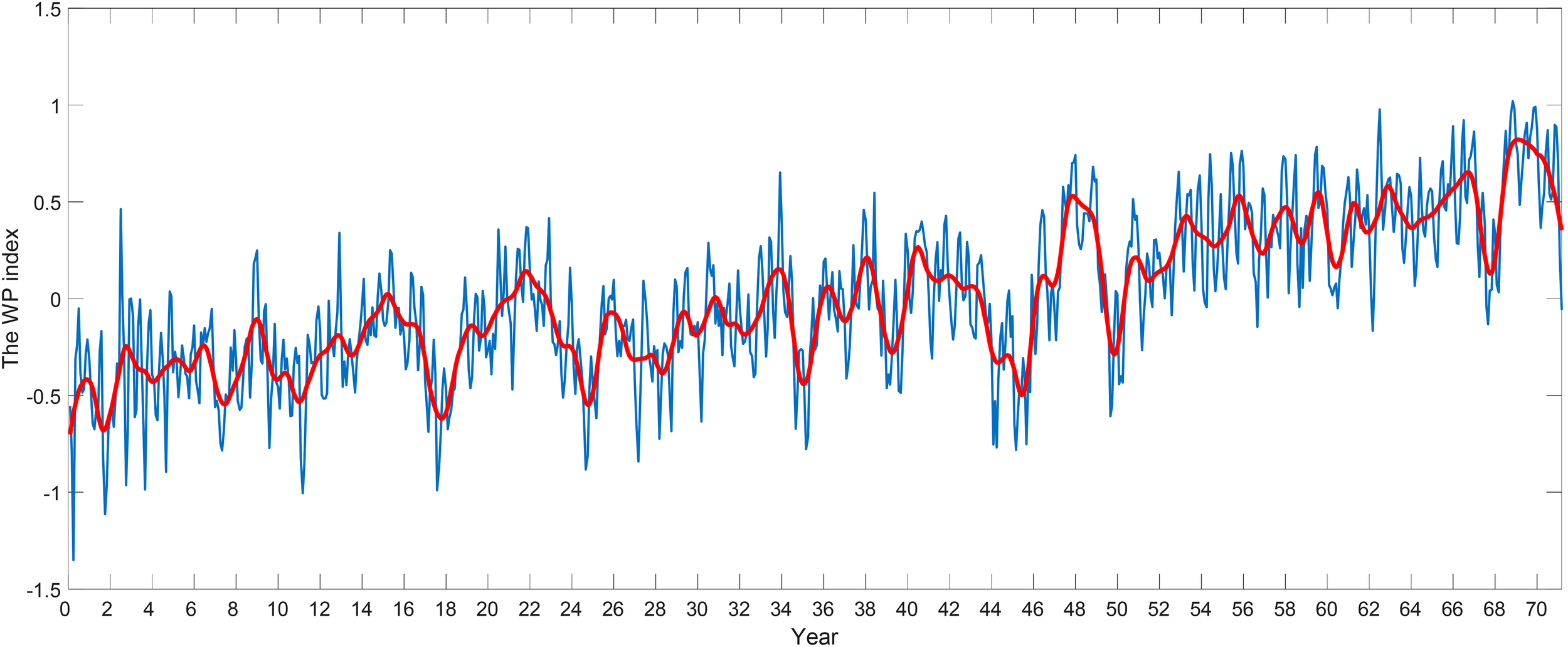
Original time series (blue line) and filtered time series (red line) of WP index.
Figure 6

Original time series (blue line) and filtered time series (red line) of WWI index.
Therefore, the CWT is needed for each characteristic index after filtering to obtain the corresponding the wavelet power spectrum. The periodic variation characteristics of each factor influencing the WPSH can be obtained more accurately, as shown in Figure 7. The wavelet energy spectrograms of the Nino3, MPSST, WP, and WWI indexes show that these influencing factors also have obvious IAV characteristics, mainly in the quasi-two-to-three-year oscillation period of about 16–32 months, the quasi-five-year oscillation period of 32–64 months, and the relatively rare quasi-eight-year oscillation period of 100 months.
Figure 7

Wavelet power spectrum of four indexes. (A) The Nino3 index (B) The MPSST index (C) The WP index (D) The WWI index.
Specifically, there are continuous high-value energy zones in the period of 16–64 months for the Nino3 index. The period of 16–32 months will be discontinuities in 71 years, while the high-value energy zones in the period of 32–64 months or so exist continuously and are distributed uniformly, which indicates that the equatorial eastern Pacific SST has a relatively obvious oscillation period: the QBO with 16–32-month interval and the quasi-four-to-five-year oscillation with 32–64 months in succession. The two cycles are stronger in the high-value energy region, which indicates that the contribution rates of the two cycles are basically the same and significant. The oscillation period is basically fixed, and there is no large deviation.
The MPSST index shows irregular high-value energy zones within 16–100 months, and the QBO period of 16–32 months occurs as with the Nino3 index. The oscillation periods of 32–64 months exist continuously. The difference is that the oscillation period of about 100 months appeared in the period of 200-600 months and coexisted with the first two periods. This shows that there are quasi-two-to-three-year, quasi-four-to-five-year, and quasi-eight-year oscillation periods in the equatorial central Pacific Ocean. In these three periods, the values of the high-energy regions of the latter two periods are higher, so their contribution rates are higher, which means their existence is more significant.
There is an irregular high-energy area of the WP index in the range of 16–100 months. The QBO period of the WP index is weaker and the irregular change is more obvious, which is a large difference from the former two indexes. Furthermore, there are more relatively low energy regions in the period of 32–64 months. The existence of three cycles is more complex. Among them, the oscillation energy period of 16–32 months is the smallest and that of 100 months is the highest. That is to say, the quasi-eight-year oscillation period of the SST in the warm pool area is more significant. The energy spectrum of the WWI index after CWT is similar to that of the Nino3 index. There is the quasi-two-to-three-year period of 16–32 months and the quasi-four-to-five-year period of 32–64 months, and the energy proportion of the high-value energy region of the two periods is very high, so the existence of the two periods is very significant. At the same time, during months 450–650, a quasi-eight-year period with high energy and significant existence appears, which indicates that the WWI index is high correlated with the Nino3 index and that both are correlated with the WPSH IAV.
3.3 Correlation analysis between interannual variability of WPSH and its influencing factors
From analyzing the time series of the WPSH and its influencing factors, we can see roughly that there is a certain correlation among them, whereupon a CWT is applied to each characteristic index. From analyzing the wavelet energy spectrogram of each index, we obtain the significant period of each index at any time and compare with the WPSH IAV to analyze its correlation. In this section, the critical value formula of correlation coefficient is used as the equation (3).
When a=0.01, tα=2.576; rc=0.0881; That is to say, when the confidence is 0.01, the critical value of the significant correlation coefficient is 0.0881, and when r > 0.0881 the correlation is significant.
The Table 1 is a table of the correlation coefficients of the WPSH intensity index and influencing factors. It can be seen that the critical value is smaller than the correlation coefficients of the four influencing factors and the WPSH intensity index, which indicates that the four factors are all significantly correlated with the WPSH intensity index. Therefore, the WPSH IAV can be studied by using the interannual anomalous changes of the SST in the equatorial latitude and three key sea areas.
Table 1
| The Nino3 index | The MPSST index | The WP index | The WWI index | |
|---|---|---|---|---|
| the WPSH intensity index | 0.5327 | 0.5603 | 0.6974 | 0.4060 |
Coefficients of correlations between WPSH intensity index and influencing factors.
Xie et al., (2009) mentioned that Indian Ocean SST has a significant impact on WPSH through the summer (June-August) after El Niño differences in spring, but we calculated the Coefficients of correlations between WPSH intensity index and Indian Ocean SST is only 0.2877, which is lower than the four factors we had selected. Moreover, we have conducted a large number of prediction experiments and found that the improved information diffusion model established using Indian Ocean SST index has significantly worse prediction performance than our previous prediction model. So we did not choose Indian Ocean SST. The reasons why the Nino4 index and the Nino West index hadn’t adopted are similar.
3.4 Time–frequency correlation analysis of WPSH and its influencing factors based on cross-wavelet transform
To date, most studies of the WPSH IAV have been focused on the correlation between single or unilateral influencing factors and the WPSH. At the same time, when studying the WPSH IAV and its relationship with influencing factors, most studies consider the time–frequency relationship and discuss the phase correlation on that basis. The results of periodic time–frequency and phase correlation in precise time series are not sufficiently accurate. It is therefore more popular to study the time–frequency and phase correlation in specific time series at the same time. With the deepening of studies of the WPSH IAV and the maturity of the air–sea coupling model, analyzing the interaction of various factors affecting the WPSH IAV will become mainstream.
A new method known as the XWT has emerged as a way to study simultaneously the correlation and phase correlation of multiple meteorological-data time series by combining wavelet analysis with cross-spectrum analysis. By synthesizing the local correlation characteristics of the time series, the time–frequency relationship of two time series is obtained, and the position correlation is also reflected. This is very suitable for analyzing and revealing the time–frequency correlation between the WPSH IAV and the anomalies of tropical SST and atmospheric circulation.
3.4.1 Correlation between WPSH and SST in eastern equatorial Pacific
Yu et al. (2008) specifically introduced how to determine the time delay correlation between different scale components of two time series in the cross wavelet transform method by using the arrow direction. So the time delay correlation between the components of each scale in two time series can be determined by the arrow direction of the phase difference. Figures 8A, B show the cross-wavelet energy spectrum and wavelet coherence spectrum of the WPSH intensity index and Nino3 index, respectively. From Figure 8, we can see that the high-value energy region of the WPSH intensity index and Nino3 index correspond to each other on the period of 32–64 months, and there is good correlation between them. At the same time, it can be seen that the phase difference between them is 315 ± 45°, which means that on the time scale of 32–64 months, the Nino3 index is ahead of the WPSH intensity index by 7/8 cycles. Meanwhile, in the time series of months 200–400 and 600–800, based on the direction indicated by the vectors in this area, the phase difference between the two indexes is 270 ± 45°, indicating that the Nino3 index is 3/4 cycles ahead of the WPSH intensity index. Finally, in the time series of months 200–600, there is still a high-value area on the period of 128 months, which means that the correlation between them is significant. Furthermore, based on the direction indicated by the vectors in this area, the phase difference is 270 ± 45°, which shows that on this time scale, the Nino3 index is 3/4 cycles ahead of the WPSH intensity index.
Figure 8

Cross-wavelet energy spectrum (A) and wavelet coherence spectrum (B) between WPSH intensity index and Nino3 index.
In summary, in the period scale of 32–64 months, after 12–24 months of SST enhancement in the eastern equatorial Pacific Ocean, the WPSH began to strengthen. In the whole time series, within the period scale of 32–64 months, the WPSH began to strengthen about 3/4 cycles after the enhancement of the SST in equatorial eastern Pacific. In the period of 200–500 months, on the period scale of 128 months or so, the WPSH began to strengthen about 3/4 cycles after the enhancement of the SST in equatorial eastern Pacific.
3.4.2 Correlation between WPSH and SST in central equatorial Pacific
As shown in Figures 9A, B, we can see that within the range of significance test in 200-800 months, the high-value energy region of the WPSH intensity index and Nino3 index correspond to each other in the period scale of 32–64 months, and there is good correlation between them. At the same time, based on the direction indicated by the vectors in this area, it can be seen that the phase difference between them is 330 ± 30°, which means that on the time scale of 32–64 months, the MPSST index is ahead of the WPSH intensity index by 11/12 cycles. Meanwhile, in the time series of months 300–400 and 550–650, based on the direction indicated by the vectors, the phase difference between the two indexes is 270 ± 45° in the period scale of 16–32 months, indicating that the MPSST index is 3/4 cycles ahead of the WPSH intensity index. Finally, in the time series of months 200–500, there is still a high-value area in the period scale of 128 months, which means that the correlation between them is significant. Furthermore, the phase difference is 270 ± 45° based on the direction indicated by the vectors in this area, which shows that within this time scale, the MPSST index is 3/4 cycles ahead of the WPSH intensity index.
Figure 9
Cross-wavelet energy spectrum (A) and wavelet coherence spectrum (B) between WPSH intensity index and MPSST index.
In summary, in the period scale of 16–32 months, the WPSH began to strengthen about 3/4 cycles after the enhancement of the SST in central equatorial Pacific. Within the period scale of 32–64 months, the WPSH began to strengthen about 11/12 cycles after the enhancement of the SST in central equatorial Pacific. On the period scale of 128 months or so, the WPSH began to strengthen about 3/4 cycles after the enhancement of the SST in central equatorial Pacific.
3.4.3 Correlation between WPSH And SST in warm pool area
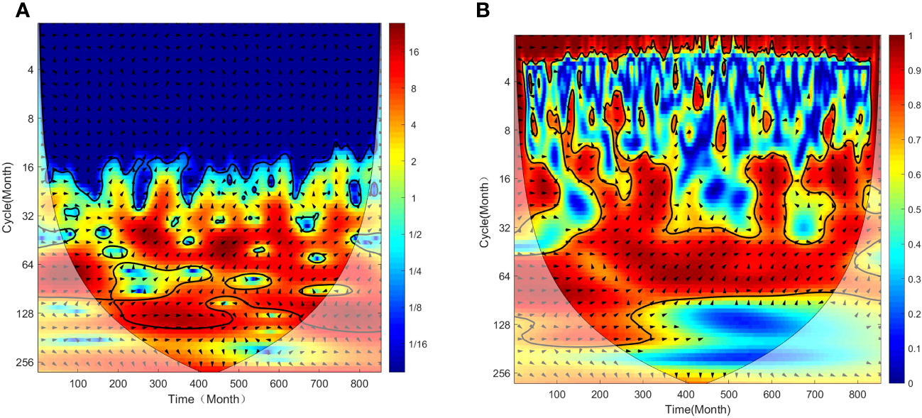
As shown in Figures 10A, B, the analysis progress of the cross-wavelet energy spectrum and wavelet coherence spectrum between the WPSH intensity index and the WP index is similar with that in sections 3-d-1 and 3-d-2 and is not elaborated here.
Figure 10

Cross-wavelet energy spectrum (A) and wavelet coherence spectrum (B) between WPSH intensity index and WP index.
In summary, in the period scale of 16–32 months, based on the direction indicated by the vectors in this area, the WPSH began to strengthen about 1/4 cycles after the enhancement of SST in the warm pool area. Within the period scale of 32–64 months, the WPSH began to strengthen about 1/4 cycles after the enhancement of SST in the warm pool area. On the period scale of 128 months or so, the WPSH began to strengthen about 7/8 cycles after the enhancement of the SST in the warm pool area.
3.4.4 Correlation between WPSH and western wind at equatorial latitude
As shown in Figures 11A, B, the analysis progress of the results of the cross-wavelet energy spectrum and wavelet coherence spectrum between the WPSH intensity index and WWI index is similar with that in sections 3-d-1 and 3-d-2 and is not elaborated here.
Figure 11

The cross-wavelet energy spectrum (A) and wavelet coherence spectrum (B) between WPSH intensity index and WWI index.
In summary, in the period scale of 16–32 months, the WPSH began to strengthen about 3/4 cycles after the enhancement of the western wind at equatorial latitudes based on the direction indicated by the vectors in this area. Within the period scale of 32–64 months, the WPSH began to strengthen about 7/8 cycles after the enhancement of the western wind at equatorial latitudes. On the period scale of 128 months or so, the WPSH began to strengthen about 7/8 cycles after the enhancement of the western wind at equatorial latitudes.
The above analysis shows that the WPSH has a quasi-two-to-three-year oscillation period of 16–32 months, a quasi-four-to-six-year oscillation period of 32–64 months, and a quasi-10-year oscillation period of 128 months. Furthermore, its IAV is related to the abnormal changes of SST in the three key regions, as well as the change of the westerly wind at equatorial latitudes. It can also be seen that the quasi-two-to-three-year oscillation period of the WPSH increased after 400 months, which is the 1980s and 1990s. This is because the SST in the warm pool area and the forcing effect of the latitude-westerly Hadley circulation strengthened, which increased the influence of the heat-source effect of the mainland on the intensity change of the WPSH.
From the time-lag correlation between the WPSH and its influencing factors, the WPSH IAV is due to the abnormal changes of tropical SST and atmospheric circulation, and vice versa. The XWT results show that regardless of the oscillation period of the WPSH IAV, the variation of the SST in eastern equatorial Pacific is always ahead of that in central equatorial Pacific and the warm pool, while the variation of the western wind at equatorial latitudes is ahead of the former three, which also shows that the anomalous variation of the atmospheric circulation impacts greatly the variation of WPSH IAV. Specifically, the weakening of the WPSH strengthens the westerly wind at equatorial latitudes on the south side of the WPSH. This strengthened westerly wind causes warmer water to diffuse eastward, which causes the SST in eastern equatorial Pacific to rise and propagate westward. As a result, the SST in equatorial central Pacific and the warm pool area increases abnormally, and the sea water warms up the atmosphere while it heating up. Under the action of the Hadley circulation, the WPSH begins to increase. With the increase of the WPSH, the westerly wind at equatorial latitudes decreases and the SST in equatorial eastern Pacific decreases. At the same time, the SST in equatorial central Pacific and the warm pool decreases anomalously and the Hadley circulation weakens, so the WPSH weakens to the south. This complete cycle of the WPSH IAV is shown in Figure 12.
Figure 12

Complete cycle of interannual variations of WPSH.
4 Establishing prediction model of interannual variability of WPSH based on improved information diffusion method
4.1 Estimation of information diffusion of WPSH intensity index
Suppose that is a knowledge sample of the above four factors (Nino3, MPSST, WP, and WWI) affecting the WPSH intensity index from January 1948 to December 2008, and the observed values Xi are recorded as li. Then suppose that . When X is incomplete, there exists a function μ(x) to diffuse the information obtained by the point li with unit magnitude according to the magnitude of μ(x). Moreover, the distribution of the original information obtained by diffusion can better reflect the general law of X, which is known as the principle of information diffusion. According to this principle, the estimation of the parent probability density function is known as diffusion estimation. The exact definition of diffusion estimation is as follows.
Let μ(x) be a Borel measurable function defined above , where d>0 is a constant and , so
This is a diffusion estimate of the parent probability density function f(l). The equation μ(x) is known as the diffusion function, and d is known as the window width.
According to Eq. (4), the key to diffusion estimation is the diffusion function μ(x). Huang (1997) used molecular diffusion theory to derive the normal diffusion function, namely
By substituting Eq. (5) into Eq. (4), the normal diffusion estimates of the parent probability density function f(l) are obtained, namely:
where h is known as the empirical window width, the formula for which is deduced according to the principle of proximity selection:
where a = min(li), b = max(li) (), and n is the sample size.
4.2 Establish fuzzy mapping relationship for intensity index of WPSH
For an “input–output” system, Ω is the parent and the input and output components are recorded as x and y, respectively. The output is the predicted value of the WPSH intensity index, and the input comprises the four factors that affect the WPSH intensity index (Nino3, MPSST, WP, and WWI) and the historical observations of the WPSH intensity index. This X×Y is the domain space of the input and output set. The experience window widths dx and dy of the input and output components can be obtained from Eq. (4). The probability density function f(x,y) of the parent Ω reflects the information distribution density of the points (x,y) in the space.
Based on probability theory and fuzzy set theory, for the input–output system, when given input x, a fuzzy set can be defined to represent the output y, and its membership function is σ(y) = f(x,y). In this way, a diffusion estimate of the parent Ω probability density function can be obtained by using the principle of information diffusion from known samples, and a mapping relationship can be established between the input and output components.
In information diffusion, small-sample data are regarded as “information injection points” scattered in the domain space X×Y of the “input–output.” Through set-valued processing, each set of sample data is expanded into the representation of fuzzy sets of multiple sample points. Aiming at the ambiguity and fuzziness of the “surrounding” boundary of sample points (x,y), the data are transmitted. In the input and output spaces, sets of “monitoring points” and are introduced, and the equation is:
where and are discrete points with equal step increments. In this way, the monitoring-point space U×V constitutes a grid distributed in the “input–output” space. The information about the “information injection points” is spread reasonably and effectively to the whole monitoring-point space through the information diffusion formula.
When the information matrix Qi of a single sample (xi,yi) at U×V is composed, the original information matrix of the sample population is:
where num is the sample point capacity. From , in which Qlx comprises the column vectors of the original information matrix, the fuzzy relation matrix can be obtained. The transformation relationship between the two matrices is:
Assuming input xi and distributing information, a fuzzy set can be obtained as:
where and . The fuzzified input and the fuzzy relation matrix R are combined fuzzily as:
Finally, the output value is obtained by deblurring:
4.3 Establishing optimum window width for WPSH intensity index
Although the empirical window width combined with the principle of fuzzy mapping has better applicability and feasibility than does the classical Kriging interpolation method in dealing with sparse SST data, it is difficult to solve the default problem of asymmetric and non-normal data. Given the defect that the empirical window width is not suitable for a non-normal distribution, an iterative formula for the optimal window width is obtained according to the criterion of minimum mean square error of matrix distribution estimation:
where max() is the maximum function, min() is the minimum function, and mean() is the average function. Suppose that ϵ is a small normal number. If any of holds, then the iteration is stopped and the optimal window width is chosen.
The optimal window width is suitable for multiple distributions and is more accurate in information diffusion estimation. However, when dealing with the different window widths obtained at different sample points in Eq. (14), only the average is used for iterative approximation, which inevitably leads to a local optimum. We must find an improved method to find a suitable window width for all sample points. GA is optimization algorithms that have been used widely in recent years. Their characteristics are global search and parallel computing, so they have good parameter optimization ability and error convergence speed. As such, we use a GA to find the suitable window width for all sample points.
4.4 Improvement of optimal window width for WPSH intensity index based on GA
The functional relationship between the window width, the diffusion function μ(x), and the knowledge sample size n is
Because f(l) is not known when dealing with the actual problem, considering the asymptotic unbiased estimation of f(l) as being , so is used instead of f(l). To facilitate computer operation, the following second-order difference scheme is adopted:
The formula for the window width is obtained by substituting Eq. (15) into Eq. (16):
Compared with the optimal-window-width iteration of Eq. (14), Eq. (17) is more concise and clear.
Next, we use a GA to search for the optimal solution from Eq. (17). For global optimization by the GA, we assume that the maximum value of the observed values corresponding to the knowledge samples X is b, that the minimum value is a, and that the possible range of the window width d is (0,(b–a)/3]. Then, n = 200 random floating-point chromosomes are generated from the above range to form the initial population . So we set up:
This is the evaluation function, which is the key to the GA. The fitness values of all the chromosomes are ranked from small to large according to the evaluation function. The fitness value is expressed as:
where index is an ordinal number, and the value range of a is (0,1); generally, we have a = 0.6. In addition to coding, population generation, setting the evaluation function, and fitness estimation, the genetic operation steps also include population paternity selection, genetic crossover, and gene mutation. The algorithm flow, calculation principle, and detailed description are given in other relevant literature (Srinivas and Patnaik, 1994). When the population evolves into the next generation with no significant change in the evaluation function, the genetic operation is stopped, and the individual with the largest fitness value at this time is selected as the ultimate improved window width of the knowledge sample X.
5 Experimental prediction of WPSH interannual variability
5.1 Prediction experiment
After establishing the prediction model of the WPSH IAV, we carried out an experiment to predict the WPSH intensity index from January 2009. The forecast results of the WPSH intensity index for the 120-month period are shown in Figure 13, from which we see that the prediction results of the first 60 months are very good. The mean absolute percentage error (MAPE) (Hu et al., 2001) was 6.84% and the correlation coefficient (CC) was 0.9251. The three peaks and three valleys of the WPSH intensity index are forecast accurately, but the result for March 2013 is a little higher than the actual data. For months 60–90, the forecast results diverged gradually but the trend remained still accurate. The MAPE was 14.44% and the CC was 0.8507. Also, the peak of the WPSH intensity index in June 2016 was forecast accurately.
Figure 13

120-month results of WPSH intensity index forecast by present model.
After nearly 90 months, the forecast results were accurate with a CC of 0.7680, and the MAPE increased gradually. The prediction curve for months 90–115 was consistent with the actual situation. The prediction results for months 0–90 are better than those for months 90–115, but after month 90 the MAPE began to increase significantly. As an example, the actual value was nearly 0.8 times lower than the predicted value in January 2018, with a false peak. So the MAPE was 23.98% but was still less than 25%. It is also observed in Figure 13 that the prediction results are unsatisfactory after 115 months, with a large oscillation. So the effective prediction period is nearly 115 months.
To summarize, Figure 13 shows that the long-term forecast up to 115 months was accurate and the MAPE values were within 25%. This indicates that our forecast model gives accurate results.
5.2 Prediction of abnormal WPSH behavior
We performed additional experiments were to validate the prediction performance further, choosing four years (1998, 2006, 1987, and 1983) of abnormally strong WPSH intensity and five years (1984, 2000, 1994, 1999, and 1985) of abnormally weak WPSH intensity. In Table 2, the prediction results for the different periods are compared with the actual results. The short- and medium-term prediction results are accurate, and the long-term (>90 months) prediction results are acceptable.
Table 2
| Statistical test Forecast events |
Short-term (1~60months) |
Medium-term (61~90 months) |
Long-term (91~120 months) |
|||
|---|---|---|---|---|---|---|
| CC | MAPE | CC | MAPE | CC | MAPE | |
| WPSH intensity index bigger event1(1998. 06 as initial values to forecast) | 0.917 | 5.14% | 0.817 | 10.88% | 0.684 | 23.51% |
| WPSH intensity index bigger event2(2006. 07 as initial values to forecast) | 0.907 | 5.33% | 0.865 | 15.27% | 0.714 | 24.68% |
| WPSH intensity index bigger event3(1987. 07 as initial values to forecast) | 0.908 | 6.04% | 0.788 | 10.92% | 0.722 | 22.57% |
| WPSH intensity index bigger event4(1983. 08 as initial values to forecast) | 0.905 | 7.11% | 0.802 | 9.44% | 0.701 | 20.14% |
| WPSH intensity index smaller event1(1984. 07 as initial values to forecast) | 0.899 | 8.13% | 0.781 | 10.65% | 0.671 | 24.15% |
| WPSH intensity index smaller event2(2000. 06 as initial values to forecast) | 0.885 | 6.45% | 0.810 | 10.57% | 0.705 | 21.33% |
| WPSH intensity index smaller event3(1994. 08 as initial values to forecast) | 0.911 | 5.72% | 0.785 | 8.65% | 0.691 | 21.13% |
| WPSH intensity index smaller event4(1999. 06 as initial values to forecast) | 0.855 | 6.42% | 0.804 | 11.02% | 0.741 | 21.22% |
| WPSH intensity index smaller event5(1985. 07 as initial values to forecast) | 0.923 | 3.55% | 0.876 | 7.12% | 0.813 | 18.45% |
| The average | 0.901 | 5.99% | 0.814 | 9.82% | 0.716 | 21.91% |
CC and MAPE between prediction results and actual values of different events in abnormal WPSH years.
5.3 Prediction of normal WPSH behavior
In section 5-b, the results of predicting abnormal WPSH behavior were good. We now consider predicting normal WPSH behavior to test our model further. We chose eight years in which the WPSH behaved normally (1986, 1989, 1992, 1995, 1996, 2001, 2004, and 2009). The short- and medium-term prediction results for the normal WPSH years were accurate and the MAPE values were within 10%. However, the long-term (>90 months) prediction results were not very consistent with the actual values, but the MAPE values were within 25%, which is acceptable.
6 Discussions and conclusions
6.1 Discussions
How to explain the quantitative relationship between the WPSH index and the East Asian rainfall index?
A lot of research pointed out that as an important member of the East Asian summer monsoon system, WPSH has a significant impact on East Asian summer precipitation due to its interannual changes (Wang and Zhi, 2015; Li X. Y. et al., 2021). The selected precipitation data is the NOAA Global Precipitation Climatology Center’s monthly precipitation dataset from January 1948 to January 2019, with a grid distance of 2.5 × 2.5, selecting the approximate location of the middle and lower reaches of the Yangtze River and its surrounding areas, with a range of 23.75 to 33.75 N and 108.75 to 123.75 E. Calculate the grid average of precipitation in this area as a precipitation index. Firstly, calculate the correlation coefficients between the WPSH intensity index, WPSH ridge line index, and WPSH western ridge point index with the precipitation index, which are 0.6613, -0.4832, and -0.3369, respectively. It can be seen that the correlation between the WPSH intensity index and the precipitation index in the middle and lower reaches of the Yangtze River is the best, and it is greater than 0.6, showing a strong positive correlation.
We further examined the correlation between the three indices of WPSH and summer precipitation in the middle and lower reaches of the Yangtze River. The Canonical Correlation Analysis (CCA) method was chosen, and the basic principle and process of this method can be seen in the relevant reference (Thompson, 2000). The variables X1,X2,X3 represented the WPSH intensity index, the WPSH ridge line index and the WPSH western ridge point index, respectively. The variables Y1,Y2,Y3 represented the precipitation in the middle and lower reaches of the Yangtze River basin in June, July, and August. Perform correlation calculations using the Canonical Correlation Analysis. The results obtained are shown in Table 3.
Table 3
| Canonical correlation | Correlation coefficients of the original two sets of variables | |
|---|---|---|
| R 1 = 0.5657 | GU(1) = 0.702 | GV(1) = 0.445 |
| GU(2) = –0.551 | GV(2) = –0.315 | |
| GU(3) = –0.215 | GV(3) = –0.531 | |
| R 2 = 0.33313 | GU(1) = –0.137 | GV(1) = 0.127 |
| GU(2) = 0.447 | GV(2) = 0.000 | |
| GU(3) = –0.817 | GV(3) = 0.413 | |
| R 3 = 0.15298 | GU(1) = 0.631 | GV(1) = 0.227 |
| GU(2) = –0.457 | GV(2) = –0.174 | |
| GU(3) = –0.331 | GV(3) = –0.567 | |
The Canonical Correlation Analysis results.
The bold indicates the value of Canonical correlation.
The results obtained from the canonical correlation analysis are tested for significance. The first canonical correlation coefficient R is significant. So, the first pair of typical variables is:
Calculate the correlation coefficient between the first typical variable and the original two sets of variables:
It can be analyzed that there is a significant positive correlation between the WPSH intensity index and summer precipitation in the Yangtze River Basin. In addition, there is a negative correlation between the WPSH ridge line and the WPSH western ridge point index with the summer precipitation. Comparing the correlation coefficients, it is still the strongest correlation between the WPSH intensity index, which is why we chose the intensity index among the three indices. The relationship between the subtropical high and summer precipitation in the Yangtze River Basin is mainly reflected in June and August, which is closely related to the precipitation in these two months.
Furthermore, EOF decomposition was performed on precipitation distribution field in the summer (June-August).The variance contribution of the first four feature mode converges relatively quickly, with their cumulative variance contribution accounting for 80.52% of the entire original field. The first four modes of the precipitation distribution field can basically reflect the main characteristics of the precipitation distribution field. In order to further understand the correlation between the precipitation distribution field and the WPSH intensity index, the first mode PC1, the second mode PC2 and the third mode PC3 obtained from the EOF decomposition of the precipitation distribution field are used for correlation analysis respectively with the WPSH intensity index, and the corresponding correlation coefficients are 0.7369, 0.6722 and -0.5841. Therefore, it can be known that there is also a strong correlation between the precipitation distribution field in the middle and lower reaches of the Yangtze River and the WPSH intensity index.
We use correlation, Canonical Correlation Analysis and composite analyses to quantify the WPSH intensity index in our study which has strong correlation with East Asian summer climate, especially with the summer precipitation in the middle and lower reaches of the Yangtze River. It is more closely related, especially in June and August.
Why we chose the WPSH intensity index to research in our paper?
There are many indicators to characterize the WPSH. The intensity index we use here is similar to the subtropical high area index, which is used to describe the intensity change of the subtropical high; In addition, there are also the ridge index and western ridge point index of the subtropical high mentioned in the previous paper such as Su and Xue (2010) and Su et al. (2017). The ridge index mainly characterizes the changes in the north-south position of the subtropical high and the northward jump and the western ridge point index of the subtropical high mainly represents the changes in the east-west position of the subtropical high. Based on the above question, the WPSH intensity index showed stronger correlation than the other two indexes. So we had chosen the WPSH intensity index. In the next step, we will use similar methods to further study the relationship between the ridge index and western ridge index of the subtropical high with the influencing factors of the East Asian monsoon system, and further test the predictive effect of the Improved Information Diffusion Model. We will reveal the interannual variation patterns of the subtropical high from more dimensions and levels. Of course, if we replace the intensity index with the ridge index or the western ridge index, the corresponding most important influencing factors may also change. This will be the focus of our next work. These indices represent different characteristics of the subtropical high, such as the intensity index representing the intensity of the WPSH, and the ridge index representing the north-south position of the WPSH northern jump. Therefore, it is not necessary to determine which index is better or which index is worse, but rather the different characteristics of the system represented by different indices.
Only data from 1979 onward, the meteorological observation satellite data began to be included in objective analysis data, why we also use the data before 1979?
Because a large number of previous studies (He and Gong, 2002; Wu and Zhou, 2008; Jiang et al., 2011; Chen et al., 2020) have also used pre 1979 data to study the interannual and interdecadal changes of WPSH, So we believe that this data issue should have little impact on our research. We had conducted sensitivity tests specifically on whether to use data before 1979. After removing the data before 1979, we conducted correlation analysis on cross wavelet and wavelet coherence, and re-established the Improved Information Diffusion Model using data after 1979 as input. However, its prediction performance was slightly worse than the previous model in our paper, but the difference was small. Through this sensitivity test, we believe that the data before 1979 had little impact on our research results. However, we will also consider whether we can do some data preprocessing to thoroughly address the impact of this climate change event and the issue of unreliable data before 1979, which is also the focus of our next work.
6.2 Conclusions
The main focus of our paper is the correlation between the WPSH IAV and the anomalies of tropical SST and atmospheric circulation, as well as on predicting the WPSH IAV.
-
From processing the monthly average data of the 500-hPa potential height obtained by NCEP from January 1948 to January 2019 for 854 months, the intensity index representing the magnitude of the WPSH intensity was obtained.
-
From the results of previous studies (Wang and Zhou, 2004; Yu et al., 2008; Matsumura et al., 2015), the SST in three key regions and the circulation variation in the westerly region at equatorial latitudes were selected as the factors affecting the WPSH IAV, which were defined as the Nino3, MPSST, WP, and WWI indexes.
-
An XWT was applied to the time series of the WPSH intensity index and influencing factors after the CWT. By observing the distributions of the energy extrema and arrows, it was found that there are quasi-two-to-three-year and quasi-five-year oscillation periods in the whole time series.
-
After determining the influencing factors, we established a prediction model for the IAV of the WPSH intensity index by means of the improved information diffusion method based on a GA, and we conducted an experiment to predict the WPSH IAV intensity index. The experimental results showed that our prediction model was accurate in predicting the trend of interannual change and good in predicting the interannual change within 84 months. The correlation coefficient was 0.8507 and the MAPE was within 14.44%. However, after 84 months, the divergence was somewhat severe, and the accuracy of the forecast decreased slightly, but the correlation coefficient was 0.7680 and the MAPE still did not exceed 25%, which was still acceptable. We also used abnormal and normal WPSH years as different starting points and conducted additional prediction experiments. It was seen that the different starting points had little influence on the prediction results, thereby showing the stability of our model.
Chao and Tianjun (2014) carried out the two IAV modes of WPSH which are simulated by 28 CMIP5–AMIP models, but the simulated anomalous WPSH was displaced northeastward and was slightly weaker compared with the observation. Moreover, they mainly simulated two annual variability models, without real-time prediction. Zhou et al. (2009) carried out GAMIL CliPAS experiments to predict the WPSH IAV in summer. They performed an 18-year prediction experiment for the standardized WPSH index from 1980 to 1998 (their Figure 4). The correlation coefficient between the predicted value and the real value was 0.56, which was significantly lower than our correlation coefficient of 0.74.
The WPSH and the 2-3, 4-5, and 8-10 year cycles of ocean variability referred to in this study are well known in the weather and climate field and previous researchers have also conducted many studies in this area. But these are all studies of statistical periodicity, which are statistical analysis and power spectrum analysis. The characteristics of cross wavelet analysis and wavelet coherence in our paper not only confirm the correctness of the oscillations discovered by previous researchers, but also map these periods to the specific year or even specific month. This means it can apply generalized periodic changes to the specific year and month (Narasimha and Bhattacharyya, 2010). The characteristic of wavelet analysis itself is signal amplifier, which can not only reveal the existence of fixed periods in a long time series, but also can be specific to a certain year whose 3-5 year or 2-3 year period is the strongest, and can also reveal which years have weaker periodicity. In addition, according to previous research (Baddoo et al., 2015), it can also be found that the cross wavelet and wavelet coherence methods can not only analyze the degree of correlation between two signals, but also obtain the phase relationship of the signals in the time-frequency space. Therefore, wavelet coherence can be used to detect common local temporal oscillations in non-stationary signals. And one time series affecting another time series, the phase of wavelet cross spectrum can be used to identify the relative lag between two time series. This function of locating temporal oscillations and determining phase lag is not previously disclosed. Moreover, this function provides rationality for the selection of predictive factors for our subsequent Improved Information Diffusion Model. In addition, the Improved Information Diffusion Model we have established for the interannual variation of WPSH has certain innovative value and had achieved good forecasting results. The main reason is that our information diffusion method has improved the quantity and quality of data samples. So this new prediction model for interannual variations of the subtropical high is also one of the most important innovations of our article.
Because of the interdecadal variability of the WPSH and SST in the tropical Pacific Ocean in the 1980s, we should also consider how that SST variation influenced the WPSH. Also worth considering is whether the information diffusion method can be improved to obtain better medium- and long-term forecasts. We will focus on these issues in future work.
Many meteorological and marine dynamic systems are chaotic systems with many influencing factors and complicated mechanisms. It is difficult for us to write their accurate dynamic equations, so we introduce statistics or machine learning methods to mine the correlation between systems from big data. In this sense, statistical modeling and machine learning or deep learning do not have a deep understanding of physical mechanisms, which is a common problem. In our future work, we will conduct sensitivity experiments on the parameters in the Improved Information Diffusion Model to discuss their physical significance. Alternatively, we will add constraints or boundary conditions that include dynamic mechanisms to the Improved Information Diffusion Model, which can add physical mechanism explanations to our model. This is the focus of our next work.
Statements
Data availability statement
The original contributions presented in the study are included in the article/supplementary materials. Further inquiries can be directed to the corresponding authors.
Author contributions
Conceptualization: MH. Methodology: JS. Software: YZ. Writing—original draft preparation: ZG. Writing—review and editing: LQ. All authors have read and agreed to the published version of the manuscript
Funding
This study is supported by the Natural Science Foundation of Hunan Province (2023JJ10054) and National Natural Science Foundation of China (No. 42375016; No. 41875061; No. 41775165; 51609254).
Conflict of interest
The authors declare that the research was conducted in the absence of any commercial or financial relationships that could be construed as a potential conflict of interest.
Publisher’s note
All claims expressed in this article are solely those of the authors and do not necessarily represent those of their affiliated organizations, or those of the publisher, the editors and the reviewers. Any product that may be evaluated in this article, or claim that may be made by its manufacturer, is not guaranteed or endorsed by the publisher.
References
1
Baddoo T. D. Guan T. D. Zhang D. Andam-Akorful S. A. (2015). Rainfall variability in the Huangfuchuang watershed and its relationship with ENSO. Water7 (7), 3243–3262. doi: 10.3390/w7073243
2
Chao H. Tianjun Z. (2014). The two interannual variability modes of the Western North Pacific Subtropical High simulated by 28 CMIP5–AMIP models. Clim. Dyn.43, 2455–2469. doi: 10.1007/s00382-014-2068-x
3
Chao H. Zhou T. J. Wu B (2015). Key sea areas and influence mechanism affecting the interannual variability of subtropical high over the Northwest Pacific in summer. Acta Meteorol. Sin. (in Chinese) 73 (05), 940–951.
4
Chen S. Q. Xu F. Li Y. J. Du J. M. Xu T. F. Ji Q. Q. et al . (2020). Summer SST in the Northwest Pacific in the past 70 years and its correlation with the variation of the western Pacific subtropical high. J. Trop. Meteorol.6, 846–854. doi: 10.16032/j.issn.1004-4965.2020.075
5
Choi W. Kim K. Y. (2019). Summertime variability of the western North Pacific subtropical high and its synoptic influences on the East Asian weather. Sci. Rep.9 (1), 1–9. doi: 10.1038/s41598-019-44414-w
6
Chowdary J. S. Xie S. P. Tokinaga H. Okumura Y. M. Kubota H. Johnson N. et al . (2012). Interdecadal variations in ENSO teleconnection to the Indo-Western Pacifc for 1870-2007. J. Climate25, 1722–1744. doi: 10.1175/JCLI-D-11-00070.1
7
He R. Chen Y. Huang Q. Wang W. P. Li G. F. (2021). Forecasting summer rainfall and streamflow over the Yangtze river valley using western Pacific subtropical high feature. Water13 (18), 2580–2588. doi: 10.3390/w13182580
8
He X.-Z. Gong D.-Y. (2002). Interdecadal change in Western Pacific Subtropical High and climatic effects. J. Geograph. Sci.12, 202–209. doi: 10.1007/BF02837475
9
He C. Zhou T. (2015). Decadal change of the connection between summer western North Pacifc Subtropical High and tropical SST in the early 1990s. Atmos. Sci. Let.16, 253–259. doi: 10.1002/asl2.550
10
Hong M. Zhang R. Zhang H. Ma C. Ge J. Zhao L. et al . (2014). The correlation between the Intraseasonal abnormal activities of the subtropical high over the western Pacific and the time delay of the Asian summer monsoon system. Trans. Atmos. Sci. (in Chinese) 37 (06), 705–714.
11
Hu T. S. Lam K. C. Ng S. T. (2001). River flow time series prediction with a range-dependent neural network. Hydrol. Sci. J.46, 729–745. doi: 10.1080/02626660109492867
12
Huang C. (1997). Principle of information diffusion. Fuzzy Sets Syst.91, 69–90. doi: 10.1016/S0165-0114(96)00257-6
13
Huang C. (2001). Information matrix and application. Int. J. Gen. Syst.30, 603–622. doi: 10.1080/03081070108960737
14
Jiang X. Li Y. Yang S. Wu R. (2011). Interannual and interdecadal variations of the South Asian and western Pacific subtropical highs and their relationships with Asian-Pacific summer climate. Meteorol. Atmos. Phys.113, 171–180. doi: 10.1007/s00703-011-0146-8
15
Li C. Lu R. Dunstone N. (2021). Prediction of the western north pacific subtropical high in summer without strong ENSO forcing. J. Meteorol. Res.35, 101–112. doi: 10.1007/s13351-021-0113-3
16
Li X. Y. Lu R. Y. Li G. (2021). Different configurations of interannualvariability of the western North Pacific subtropical high and East Asian westerly jet in summer. Adv. Atmos. Sci. doi: 10.1007/s00376-021-0339-0
17
Matsumura S. Horinouchi T. (2016). Pacifc Ocean decadal forcing of long-term changes in the western Pacifc subtropical high. Sci. Rep.6, 37765. doi: 10.1038/srep37765
18
Matsumura S. Sugimoto S. Sato T. (2015). Recent intensification of the western Pacific subtropical high associated with the East Asian summer monsoon. J. Climate28, 2873–2883. doi: 10.1175/JCLI-D-14-00569.1
19
Narasimha R. Bhattacharyya S. (2010). A wavelet cross-spectral analysis of solar–ENSO–rainfall connections in the Indian monsoons. Appl. Comput. Harmonic Anal.28 (3), 285–295. doi: 10.1016/j.acha.2010.02.005
20
Park J.-Y. Jhun J.-G. Yim S.-Y. Kim W.-M. (2010). Decadal changes in two types of the western North Pacifc subtropical high in boreal summer associated with Asian summer monsoon/El Nino-Southern Oscillation connections. J. Geophys. Res.: Atmos.115, D21129,1775–1789. doi: 10.1029/2009JD013642
21
Ren Y. Zhou B. Song L. Xiao Y. (2017). Interannual variability of western North Pacific subtropical high, East Asian jet and East Asian summer precipitation: CMIP5 simulation and projection. Quaternary Int.440, 64–70. doi: 10.1016/j.quaint.2016.08.033
22
Srinivas M. Patnaik L. M. (1994). Adaptive probabilities of crossover and mutation in genetic algorithms. IEEE Trans. Syst. Man Cybernetics24 (4), 656–667. doi: 10.1109/21.286385
23
Stowasser M. Wang Y. Hamilton K. (2007). Tropical cyclone changes in the Western North Pacific in a global warming scenario. J. Climate20, 2378–2396.
24
Su T. Xue F. (2010). The intraseasonal variation of summer monsoon circulation and rainfall in East Asia. Chin. J. Atmos. Sci.34 (3), 611–628. doi: 10.3878/j.issn.1006-9895.2010.03.13
25
Su T. Xue F. Chen M. Dong X. (2017). A mechanism study for the intraseasonal oscillation impact on the two northward jumps of the western Pacific subtropical high. Chin. J. Atmos. Sci.41 (3), 437–460. doi: 10.3878/j.issn.1006-9895.1609.16125
26
Sui C. H. Chung P. H. Li T. (2007). Interannual and interdecadal variability of the summer time wstern North Pacific subtropical high. Geophys. Res. Lett.34 (11), L11701,2245–2258. doi: 10.1029/2006GL029204
27
Sun C. Shi X. Yan H. Jing Q. X. Zeng Y. X. (2022). Forecasting the June ridge line of the western Pacific subtropical high with a machine learning method. Atmosphere13 (5), 660–668. doi: 10.3390/atmos13050660
28
Thompson B. (2000). “Canonical correlation analysis,” in Reading and understanding MORE multivariate statistics. Eds. GrimmL. G.YarnoldP. R. (Encyclopedia of statistics in behavioral science: American Psychological Association), 285–316.
29
Wang B. Wu R. G. Fu X. H. (2000). Pacific-East Asian teleconnection: How does ENSO affect East Asian climate? J. Clim.13, 1517–1536. doi: 10.1175/1520-0442(2000)013<1517:PEATHD>2.0.CO;2
30
Wang H. X. Zhi X. F. (2015). Statistical downscaling research of precipitation forecast based on TIGGE multimodel ensemble. J. Meteorol. Sci.35 (4), 8–17.
31
Wang C. Zhou L. (2004). Interannual variability of the subtropical high over the western Pacific and its correlation with ENSO. J. Trop. Meteorol. (in Chinese) 2004 (02), 137–144.
32
Wu B. Zhou T. J. (2008). Oceanic origin of the interannual and interdecadal variability of the summertime western Pacifc subtropical high. Geophys. Res. Lett.35, L13701. doi: 10.1029/2008GL034584
33
Xiang B. Wang B. Yu W. Xu S. (2013). How can anomalous western North Pacifc subtropical high intensify in late summer? Geophys. Res. Lett.40, 2349–2354. doi: 10.1002/grl.50431
34
Xie S. P. Hu K. M. Hafner J. Tokinaga H. Du Y. Huang G. et al . (2009). Indian Ocean Capacitor Effect on Indo-Western Pacific Climate during the Summer following El Niño. J. Clim.22, 730–747. doi: 10.1175/2008JCLI2544.1
35
Yu D. Zhang R. Hong M. Liu K. Wang H. Gui Q. (2008). Time delay correlation analysis between the convection activity in the central equatorial Pacific and the westward extension of the western Pacific subtropical high. Adv. Mar. Sci. (in Chinese) 2008 (03), 292–304. doi: 10.3724/SP.J.1047.2008.00014
36
Zhang D. Martin G. M. Rodríguez J. M. Ke Z. J. Chen L. J. (2020). Predictability of the western north Pacific subtropical high associated with different ENSO phases in Glosea5. J. Meteorol. Res.34, 926–940. doi: 10.1007/s13351-020-0055-1
37
Zhou J. Sun M. Xiang J. Guan J. P. Du H. D. Zhou L. (2022). Forecasting the western Pacific subtropical high index during typhoon activity using a hybrid deep learning model. Acta Oceanol. Sin.41 (4), 101–108. doi: 10.1007/s13131-021-1965-1
38
Zhou T. Yu R. Zhang J. Drange H. Cassou C. Deser C. (2009). Why the western Pacific subtropical high has extended westward since the late 1970s. J. Climate. doi: 10.1175/2008JCLI2527.1
Summary
Keywords
western Pacific subtropical high, interannual variability, intensity index, information diffusion method, tropical sea temperature, short- and medium-term prediction
Citation
Hong M, Shi J, Zhang Y, Guo Z and Qian L (2023) Predicting the interannual variability of the subtropical high over the western Pacific Ocean based on the improved information diffusion model. Front. Mar. Sci. 10:1240768. doi: 10.3389/fmars.2023.1240768
Received
15 June 2023
Accepted
10 August 2023
Published
08 September 2023
Volume
10 - 2023
Edited by
Toru Miyama, Japan Agency for Marine-Earth Science and Technology, Japan
Reviewed by
Xiao Dong, Chinese Academy of Sciences (CAS), China; Tsuyoshi Yamaura, RIKEN Center for Computational Science, Japan
Updates
Copyright
© 2023 Hong, Shi, Zhang, Guo and Qian.
This is an open-access article distributed under the terms of the Creative Commons Attribution License (CC BY). The use, distribution or reproduction in other forums is permitted, provided the original author(s) and the copyright owner(s) are credited and that the original publication in this journal is cited, in accordance with accepted academic practice. No use, distribution or reproduction is permitted which does not comply with these terms.
*Correspondence: Jian Shi, 1206609128@qq.com; Yongchui Zhang, zyc@nudt.edu.cn
Disclaimer
All claims expressed in this article are solely those of the authors and do not necessarily represent those of their affiliated organizations, or those of the publisher, the editors and the reviewers. Any product that may be evaluated in this article or claim that may be made by its manufacturer is not guaranteed or endorsed by the publisher.