Assessment of thermocline depth bias in the Seychelles-Chagos Thermocline Ridge of the Southwestern Indian Ocean simulated by the CMIP6 models

The Seychelles-Chagos Thermocline Ridge (SCTR, 5°S-10°S, 50°E-80°E) is a unique open-ocean upwelling region in the southwestern Indian Ocean. Due to the negative wind stress curl between the equatorial westerlies and southeasterly trade winds, SCTR is known as a strong upwelling region with high biological productivity, providing a primary fishing zone for the surrounding countries. Given its importance in shaping the variability of the Indian Ocean climate by understanding the sea-air interaction and its dynamics, the simulation of SCTR is evaluated using outputs from the Coupled Model Intercomparison Project Phase Sixth (CMIP6). Compared to observations, 23 out of 27 CMIP6 models tend to simulate considerably deeper SCTR thermocline depth (defined as the 20°C isotherm depth (D20))– a common bias in climate models. The deep bias is related to the easterly wind bias in the equatorial to southern Indian Ocean, which is prominent in boreal summer and fall. This easterly wind bias produces a weak annual mean Ekman pumping, especially in the boreal fall. Throughout the year, the observed Ekman pumping is positive and is driven by two components: the curl term, is associated with the wind stress curl, leads to upwelling during boreal summer to fall; the beta term, is linked to planetary beta and zonal wind stress, contributes to downwelling during boreal spring to fall. However, the easterly wind bias in the CMIP6 increases both the positive curl and negative beta terms. The beta term bias offsets the curl term bias and reduces the upwelling velocity. Furthermore, the easterly wind bias is likely caused by the reduced east-west sea surface temperature (SST) difference associated with a pronounced warm bias in the western equatorial Indian Ocean, accompanied by the east-west mean sea level pressure gradient over the Indian Ocean. Furthermore, this study finds local wind-induced Ekman pumping to be a more dominant factor in thermocline depth bias than Rossby waves, despite CMIP6 models replicating Rossby wave propagation. This study highlights the importance of the beta term in the Ekman pumping simulation. Thus, reducing the boreal summer-to-fall easterly wind bias over the Indian Ocean region may improve the thermocline depth simulation over the SCTR region.

1 Introduction

An open ocean upwelling region in the Indian Ocean, famously known as the Seychelles-Chagos Thermocline Ridge (SCTR; Hermes and Reason, 2009; D’Addezio and Subrahmanyam, 2016; George et al., 2018; Vialard et al., 2009) or the Seychelles Dome (SD; Yokoi et al., 2008; Nagura et al., 2013) or the thermocline ridge in the Indian Ocean (TRIO; Jayakumar and Gnanaseelan, 2012; Praveen Kumar et al., 2014; Deepa et al., 2019) has been observed and analyzed by many previous studies (e.g., Xie et al., 2002; Yokoi et al., 2012; Burns and Subrahmanyam, 2016; Nyadjro et al., 2017; Sabu et al., 2021). The upwelling is primarily driven by the Ekman pumping velocity associated with the negative local wind stress curl between the southeasterly trade wind and the equatorial westerlies. The equatorial westerlies generate equatorward Ekman flow, which helps to enhance the upwelling off the equator (Xie et al., 2002). The westward propagating Rossby waves act as a remote forcing and contribute to the variation of the thermocline depth in this region (Masumoto and Meyers, 1998; Yokoi et al., 2008). The seasonal variation of the SCTR thermocline depth is mainly controlled by the wind stress variation following the Indian Ocean monsoon (Yokoi et al., 2008). The sea surface temperature (SST) is also relatively warm (26-29.5°C), with a maximum during the boreal spring (March-April) and a minimum during the boreal summer in August (Foltz et al., 2010; Fathrio et al., 2017). In this study, seasons refer to those for the Northern Hemisphere. At the surface, the westward South Equatorial Current (SEC) current dominates from the southern region up to 10°S. The eastward South Equatorial Countercurrent (SECC) appears relatively weak between the equator and 5°S (Schott et al., 2009; Vialard et al., 2009). In the subsurface, zonal velocities are predominantly westward up to 20 cm/s in the northern Madagascar Island and the meridional current has relatively little variability (Nagura and Mcphaden, 2018).

Due to the nature of the upwelling region, this area produces high biological productivity and has become a focus area for tuna fishing activity (Fonteneau et al., 2008; Kim and Na, 2022; Kim et al., 2022). Substantial annual chlorophyll-a variability with a peak in summer (June-July-August) coincided with the southeast trade wind, which mixed the nutrient-rich subsurface layer with surface waters (Dilmahamod et al., 2016; George et al., 2018). The SST variability influenced by subsurface temperature has been shown to be a significant forcing for the formation of tropical cyclones in the Indian Ocean (Xie et al., 2002; Leroux et al., 2018; Tulet et al., 2021) and affects the precipitation activity in the Indian and African region (Ummenhofer et al., 2009). The SST anomaly in this region is also suggested as an indicator of the onset of the Indian summer monsoon season. In addition, the SCTR region has received attention from major observational projects such as the Second International Indian Ocean Expedition (IIOE-2; Hood et al., 2015), Cirene Cruise (Vialard et al., 2009), the Research Moored Array for African-Asian-Australian Monsoon Analysis and Prediction (RAMA; McPhaden et al., 2009), the Indian Ocean Observing System 2 (IndOOS-2; Beal et al., 2020) and the REunion NOVative research on cyclonic RISKs programme, (ReNovRisk, Tulet et al., 2021), indicating the importance of this region for climate variability around the Indian Ocean rim countries.

Previous studies have assessed the dynamics of the SCTR region by optimizing the availability of ocean-atmosphere coupled general circulation models (CGCMs). Many studies have found that the CGCMs are still inadequate to simulate the dynamics of the SCTR (e.g. Wang et al., 2021; Zhang et al., 2023). For example, Yokoi et al. (2009) found a substantial bias in the local Ekman pumping in the SCTR region from the output of 22 models of the World Climate Research Programme (WCRP) Coupled Model Intercomparison Project Phase 3 (CMIP3) models, caused by the inability of the models to reproduce the asymmetric monsoonal winds in the region. Furthermore, using 20 models of the Coupled Model Intercomparison Project Phase 5 (CMIP5), Zheng et al. (2016) found an overestimation of thermocline depth due to an easterly wind bias along the equator. The wind bias produces a westward-propagating downwelling Rossby wave in the southern part and overestimates the thermocline dome over the SCTR region (Li et al., 2015a; Zheng et al., 2016). Nagura et al. (2013) also found that the longitudinal bias in the 14 CMIP5 models of the SCTR dome shifted to the east. This bias results from an easterly wind bias that is noticeable in summer and fall and reproduces the shallow thermocline bias in the eastern Indian Ocean (Java and Sumatra coasts) via Kelvin wave dynamics. By evaluating 21 CMIP5 models, Fathrio et al. (2017) found that the SST was too warm in the western equatorial Indian Ocean during the summer monsoon season.

The outputs of the Coupled Models Intercomparison Project Phase 6 (CMIP6), a new generation of the Coupled Models Intercomparison Project (CMIP) series, have recently been made available. The CMIP6 models include the DECK (Diagnostic, Evaluation, and Characterization of Klima) and CMIP historical simulations (1850–near present) and an ensemble of 23 endorsed Model Intercomparison Projects (MIPs) (Eyring et al., 2016). Since the dynamics in the SCTR region play an essential role in global climate variability, especially in the Indian Ocean region, the ability of CMIP6 models to simulate the SCTR region is important, whether or not the CMIP6 models show an improvement over the previous CMIP generation. This study aims to evaluate the skills of CMIP6 models to simulate the SCTR by comparing them with reanalysis data. Specifically, the objective of this study is to assess the ability of CMIP6 models in reproducing the key characteristic of SCTR region, focusing on the importance of the Ekman pumping velocity as the primary local forcing and the westward propagating Rossby wave as the remote forcing. To the best of our knowledge, this study is the first to evaluate the SCTR simulation in the newly released CMIP6 climate models.

This paper is organized as follows. A brief description of the data observations and model outputs, as well as the methods used in this study, is presented in the next section. In Section 3, we revisit the SCTR formation from the reanalysis data and present the possible mechanisms that produce the CMIP6 thermocline depth bias in simulating the annual mean state of the SCTR region. In particular, we focus on the formation of wind-induced upwelling represented by the Ekman pumping velocity and the contribution of westward propagating Rossby wave to the SCTR region represented by the thermocline depth anomaly during Indian Ocean Dipole (IOD) events. Section 4 presents the discussion, focusing on the bias of the CMIP6 models compared to the observations and the previous generation of CMIP5 models. Conclusions are given in the final section.

2 Data and methods

2.1 Data

To see the ability of the CMIP6 models to simulate the thermocline depth, defined by the 20°C isotherm depth (hereafter D20), we used the outputs from historical runs of 27 CMIP6 models. The historical simulations were forced by observed atmospheric composition changes, such as greenhouse gases, aerosols, and solar radiation (Eyring et al., 2016). The details and references for the model configurations are provided in Table 1 and are available at https://pcmdi.llnl.gov/CMIP6/. We chose the data period from 1980 to 2014 of 35 years of simulation, following the rule of thumb of at least 30 years of minimum data period to obtain a reliable estimate of statistical data identity such as the mean (WMO, 2017). To check whether the CMIP6 models show an improvement over the previous CMIP generation, we use the output of 25 CMIP5 models (Taylor et al., 2012). However, for convenience, we choose a shorter data period from 1980 to 1999 of 20 years of simulation, since our main focus is to assess the CMIP6 data simulation. For the analysis of both CMIP5 and CMIP6 simulations, we used the monthly mean historical run and regridded to 0.5° x 0.5° spatial resolutions using bilinear interpolation. The details and model configuration references for CMIP5 models are provided in Supplementary Table S1.

TABLE 1

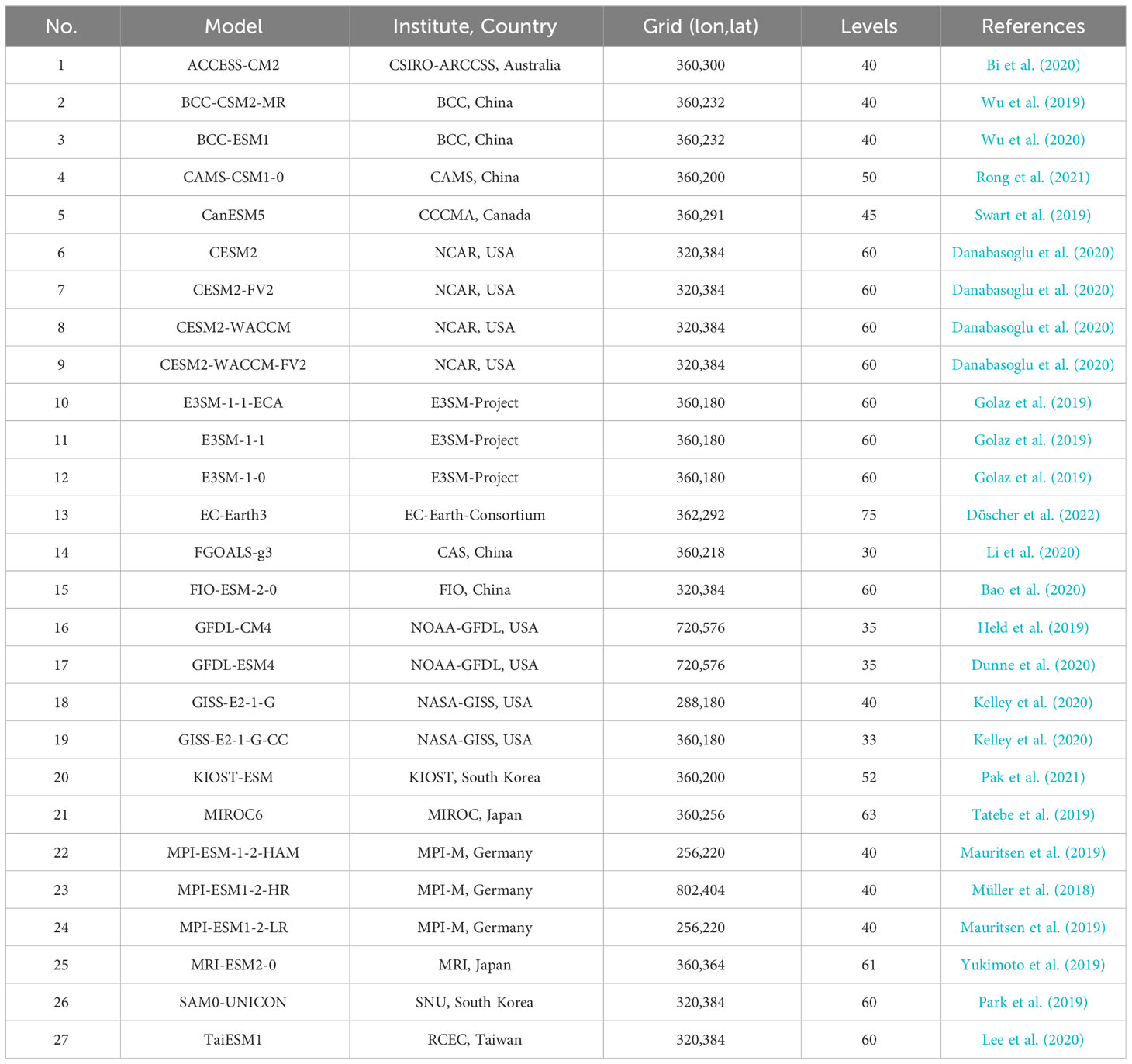
Table 1 Descriptions of the CMIP6 models used in this study.

To evaluate the skill of CMIP6 models to simulate the thermocline depth, we used monthly mean ocean temperature data from the Simple Ocean Data Assimilation version 3.4.2. (SODA3.4.2; Carton et al., 2018). SODA3.4.2 is based on the Modular Ocean Model version 5 (MOM5; Griffies, 2012), which is based on the National Oceanic and Atmospheric Administration (NOAA)/Geophysical Fluid Dynamics Laboratory (GFDL) CM2.5 coupled ocean-sea ice model (Delworth et al., 2012). It is forced by the European Centre for Medium-Range Weather Forecasts (ECMWF) ReAnalysis Interim (ERA-Interim; Dee et al., 2011) near-surface atmospheric variables in addition to downwelling shortwave and longwave radiation and includes heat and freshwater flux correction. The SODA3.4.2 uses the Coupled Ocean-Atmosphere Response Experiment version 4.0 (COARE4; Edson et al., 2013) for the bulk flux algorithms. The vertical resolution is 10 m in the upper ten levels but is coarser in the deeper ocean from the 11th to the 50th level, and the horizontal resolution of the monthly dataset is 0.5°. In addition to SODA3.4.2, we also use the reanalysis data of the EN4.2.1 (EN4; Good et al., 2013) ensemble members using the bathythermograph corrections of Levitus et al. (2009). The EN4.2.1 dataset includes subsurface temperature and salinity information, covering the period from 1900 to the present. The EN4.2.1 dataset combines data from Argo profiles, the Artic Synoptic Basin-wide Oceanography (ASBO; Curry et al., 2001) project, the Global Temperature and Salinity Profile Programme (GTSPP; Sun et al., 2010), and the World Ocean Database 2018 (WOD18; Boyer et al., 2018).

In addition to temperature data, the 10-m surface wind and mean sea level pressure were retrieved from the Climate Change Service (CCS) of the ECMWF ReAnalysis phase 5 dataset (ERA5; Hersbach et al., 2020). A major strength of ERA5 is the much higher temporal (1-hour) and spatial (31 km) resolution, which captures much finer details of atmospheric phenomena than in the previous ERA-Interim. The surface currents were retrieved from Ocean Surface Current Analyses Real-time (OSCAR) - Final 0.25 Degree Version 2.0 (https://podaac.jpl.nasa.gov/dataset/OSCAR_L4_OC_FINAL_V2.0). OSCAR is produced by Earth & Space Research (ESR, https://www.esr.org/research/oscar/). OSCAR daily ocean velocities are computed from 30-m well-mixed layer satellite-derived sea surface height gradients, combined with vector winds above the ocean and the SST gradients, by optimizing a simplified physical model for geostrophic, Ekman, and thermal wind dynamics (Bonjean and Lagerloef, 2002; ESR, 2022). It is freely available through the NASA Physical Oceanography Distributed Active Archive Center (PO.DAAC) and covers the period from 1993 to 2021. We use the same period from 1980 (1993 for ocean currents) to 2014 and the same spatial resolution of 0.5° x 0.5° for these datasets. For simplicity, we refer to these datasets as observations. Unless otherwise specified, the variables are averaged over the SCTR region from 5°S to 10°S and 50°E to 80°E and the seasons refer to that of the Northern Hemisphere. The data consisted of monthly means, and we calculated monthly anomalies by subtracting the original data to the 1980-2014 monthly climatology.

2.2 Methodology

We define the model bias for respective variables as model minus observation. We used the temperature from the SODA3.4.2 dataset to reference the D20 and SST observations. Previous studies have used the SODA dataset for a similar purpose for calculating D20 bias (e.g., Cai and Cowan, 2013; Nagura et al., 2013; Li et al., 2015a; Li et al., 2015b; Zheng et al., 2016) and is physically consistent with the observation in generating surface current dynamics in the northern Indian Ocean (Vitale et al., 2017). We defined the multi-model ensemble (MME) mean as the simple mean of 27 CMIP6 models. The thermocline depth was determined by the 20°C isothermal depth, following the previous studies of Yokoi et al. (2008); Nagura et al. (2013), and Zheng et al. (2016). The shallowest of this annual mean depth in the 5°S-10°S meridional band is referred as the thermocline dome (Yokoi et al., 2009; Nagura et al., 2013). To evaluate the performance of CMIP6 models, we calculated the annual mean of D20 bias averaged over the SCTR region. To assess the skill of CMIP6 to simulate the thermocline depth, we use the Willmott index of agreement (d). This descriptive evaluation allows for comparisons to be made across different models (Willmott, 1981; Willmott, 1982). The d ranges from 0 to 1, and when the d is closer to 1, we conclude that the respective model agrees more with the observations. In this study, we used the original form of d, defined as:

$\begin{array}{ll}d=1-\frac{{\sum }_{i=1}^n{(M_{i-}{O}_i)}^2}{{\sum }_{i=1}^n{(\left|M_i-\overline{O}\right|+\left|O_i-\overline{O}\right|)}^2}& (1)\end{array}$

where O_i and M_i are the observation and model values, respectively;$\overline{O}$ and$\overline{M}$ are the mean values for the observation and model, respectively. We also determined three models that show a high Willmott index (HWI) and three models that show low Willmott index (LWI).

We calculated the Ekman pumping velocity based on the variation of the surface wind in the SCTR region after determining the HWI and LWI. Previous studies have shown that the easterly wind bias in the CMIP5 models in the equatorial Indian Ocean is likely to produce a weak Ekman pumping. The weakened Ekman pumping produces a positive bias of the thermocline depth in the SCTR region (deeper than observed) (Yokoi et al., 2008; Yokoi et al., 2009; Cai and Cowan, 2013; Nagura et al., 2013; Li et al., 2015a; Zheng et al., 2016). Therefore, we attempted to calculate the Ekman pumping velocity using the CMIP6 dataset and compared it with the observed data.

Ekman pumping can be induced by vorticity (ζ), known as vorticity gradient-induced Ekman pumping. The total Ekman pumping equation modified by vorticity is follow (Stern, 1965; Gaube et al., 2015):

$\begin{array}{ll}\left|{\mathit{\text{W}}}_{tot}\right|=\left|\frac{1}{{\rho }_o}\mathbf{\nabla }\times \left(\frac{\mathit{\text{τ}}}{(f+\zeta )}\right)\right|& (2)\end{array}$

$\begin{array}{ll}=\left|\frac{\mathbf{\nabla }\times \mathit{\text{τ}}}{{\rho }_o(f+\zeta )}\right|+\frac{\beta {\tau }_x}{{\rho }_o{(f+\zeta )}^2}+\frac{1}{{\rho }_o{(f+\zeta )}^2}\left({\tau }_x\frac{\partial \zeta }{\partial y}-{\tau }_y\frac{\partial \zeta }{\partial x}\right)& (3)\end{array}$

$\begin{array}{ll}= W_c+W_{\beta }+W_{\zeta }& (4)\end{array}$

where ρ_o is the density of seawater (1025 kg/m³), f is the Coriolis parameter, β is the meridional gradient of the Coriolis term, and τ is surface wind stress, consisting of the zonal and meridional component τ_x and τ_y respectively. The first term in the right-hand side of Equation (3) is the Ekman pumping induced by local wind stress curl (W_c) and the second term in the right-hand side is the Ekman pumping that arise from zonal wind stress and planetary beta effect (W_β). The third term in the right-hand side of Equation (3) is related to the vorticity gradient-induced Ekman pumping or W_ζ. However, our calculations based on OSCAR data indicate that the vorticity over SCTR region (order of ~10^-7 s^-1) is relatively smaller in comparison to the Coriolis parameter (f, order of ~10^-5 s^-1) and the W_ζ(order of ~10^-8 m/s) is smaller when compared to the W_c and W_β(order of ~10^-6 m/s). Therefore, the vorticity-related term was excluded from the total Ekman pumping calculation.

Thus, the total Ekman pumping equation can be written as described in Tozuka et al. (2002) and Yokoi et al. (2008); Yokoi et al. (2009):

$\begin{array}{ll}\left|{\mathit{\text{W}}}_{tot}\right|=\left|\frac{1}{{\rho }_o}\mathbf{\nabla }\times \left(\frac{\mathit{\text{τ}}}{f}\right)\right|=\left|\frac{\mathbf{\nabla }\times \mathit{\text{τ}}}{{\rho }_{o}f}\right|+\frac{\beta {\tau }_x}{{\rho }_o{f}^2}& (5)\end{array}$

The first term on the right-hand side is proportional to the wind stress curl (hereinafter the curl term), consisting of the meridional variation of zonal wind stress and zonal variation of meridional wind stress. The second term on the right-hand side is proportional to the zonal wind stress (hereinafter the beta term).

3 Results

3.1 Thermocline depth bias in the SCTR region simulated by CMIP6 models

Figure 1 shows the thermocline depth bias from 27 CMIP6 models, represented by the difference of D20 between the models and the SODA 3.4.2 dataset. The EN4.2.1 dataset also exhibits similar results (Supplementary Figures S1, S2). Most CMIP6 models display positive D20 biases in the SCTR region, with 23 models showing positive biases and four showing negative biases. These results indicate that the thermocline depths in most CMIP6 models are deeper than observed. Specifically, out of the 27 CMIP6 models, 14 models show positive thermocline depth bias, three show negative bias, and ten models exhibit varying spatial patterns of thermocline depth bias, for example the E3SM ensemble models that demonstrate positive bias only in the SCTR region and southeastern Madagascar Island. The bias is even more prominent in certain regions than in the SCTR region. Some CMIP6 models also exhibit a strong negative D20 bias in the southern part of the Indian Ocean, near the latitude of 30°S (e.g., MPI-ESM-1-2-HAM, MPI-ESM1-2-LR, FIO-ESM-2-0, and SAM0-UNICON). The shallower-than-observed D20 in the Southern Ocean is likely caused by the overestimation of westerly wind simulation in CMIP6 climate models (Goyal et al., 2021; Deng et al., 2022), which potentially induces a relatively larger Ekman pumping velocity and shallows the thermocline depth. It is important to note that while our findings demonstrate biases in the thermocline depth across the Indian Ocean, our specific focus was on the D20 bias in the SCTR region.

FIGURE 1

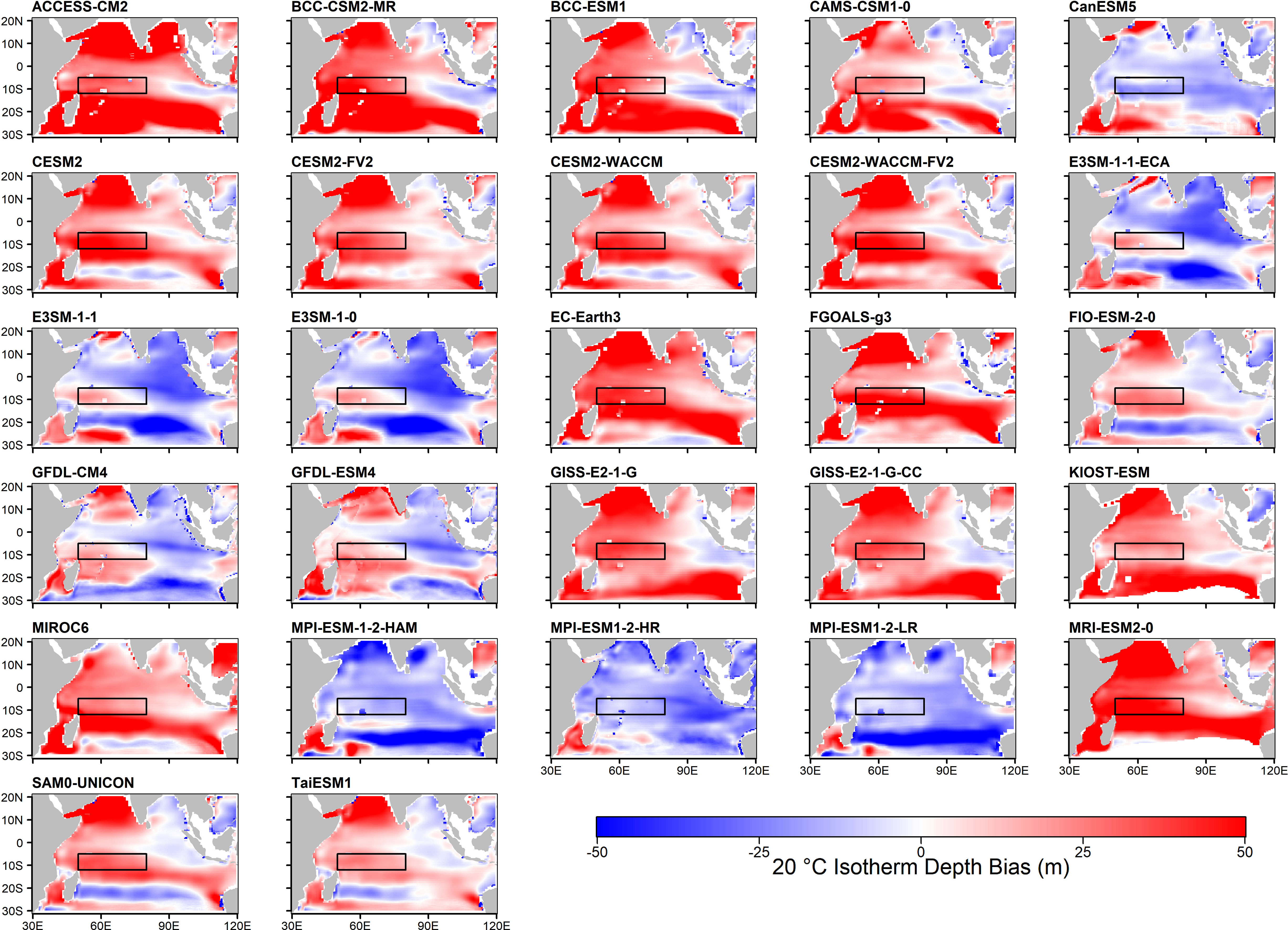
Figure 1 The annual mean of thermocline depth bias (m) from 27 CMIP6 models. Bias is calculated by model minus observation. The red color indicates positive bias, the modeled thermocline depth is deeper than observation (overestimation), and the blue color indicates negative bias, the modeled thermocline depth is shallower than observation (underestimation). The black box indicates the SCTR region from 5°S to 10°S and 50°E to 80°E.

To obtain more robust results, we calculate the D20 averaged over the SCTR region. Figure 2A shows that most CMIP6 models simulate a deeper thermocline depth compared to observations in the SCTR region. The range of simulated D20 values in the models varies from 72 m to 139 m, whereas the observed annual mean D20 in the SCTR region is around 86 m. Statistical analysis using Welch’s two-sample t-test confirms that the mean D20 in CMIP6 models significantly differs from the observation (p-value< 0.001). The three best models simulating the D20 in the SCTR region among CMIP6 models (models that show D20 bias close to zero) were simulated by E3SM-1-1, E3SM-1-0, and E3SM-1-1-ECA. The three most significant models simulating positive D20 bias in the SCTR region: MRI-ESM2-0, CESM-WACCM-FV2, and FGOALS-g3. Furthermore, the models that simulate deeper thermocline depth compared with observation have a small Willmott index of agreement value (d). Based on d, the best realistic and most unrealistic model that simulates D20 in the SCTR region is GFDL-CM4 (d = 0.61) and MRI-ESM2-0 (d = 0.23), respectively. We select GFDL-CM4, E3SM-1-0, and E3SM-1-1-ECA as the HWI. Although E3SM-1-1 (~92 m) simulates D20 slightly shallower close to observation (~86 m) compared to the GFDL-CM4 model (~94.5 m), the GFDL-CM4 (0.61) shows better d than E3SM-1-1 (0.53). We also select MRI-ESM2-0, CESM-WACCM-FV2, and FGOALS-g3 as LWI. Although the d of CESM2-FV2 (0.27) is slightly worse compared to CESM-WACCM-FV2 (0.28), the CESM-WACCM-FV2 (~130 m) simulates deeper D20 compared with CESM2-FV2 (~118 m) and thus, we select the CESM-WACCM-FV2 model as a part of LWI. The results were similar (figure not shown) when we selected E3SM-1-1 and CESM2-FV2 as included in HWI and LWI, respectively, indicating that the results are not sensitive to these changes.

FIGURE 2

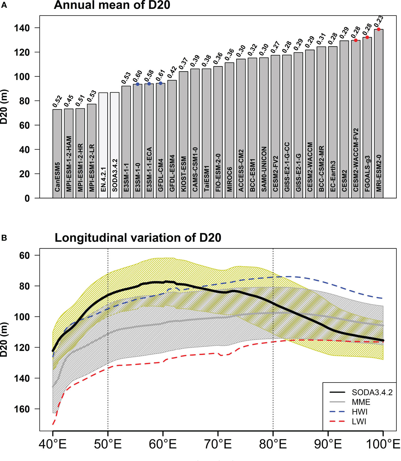
Figure 2 (A) Annual mean of D20 averaged over the SCTR region (from 5°S to 10°S and from 50°E to 80°E) from 1980 to 2014. The two light-shaded bars indicate the observed D20 from EN4.2.1 and SODA3.4.2. The blue and red dots indicate the three models that show high Willmott index (HWI) and low Willmott index (LWI), respectively. The values above the bar indicate the Willmott index of agreement (d) for the respective CMIP6 models. (B) Longitudinal variation of an annual mean of D20 averaged in 5°S to 10°S latitude band. The black and gray solid lines indicate the observation from SODA3.4.2 and multi-model ensembles (MME) mean from 27 CMIP6 models, respectively. The blue and red dash lines indicate the HWI and LWI models, respectively. In (B), the yellow shading represents one standard deviation of temporal variability from SODA3.4.2, while the gray shading represents one standard deviation of inter-model variability from CMIP6 models.

Figure 2B presents the longitudinal variation of D20 for observation, the MME mean of CMIP6 models, HWI, and LWI. In the SCTR region, the MME mean of D20 in CMIP6 models consistently indicates a significantly deeper thermocline depth compared to the observed D20 values. Furthermore, the LWI simulations also show a notable deepening of D20, surpassing even the depth indicated by the MME. Conversely, the HWI simulations exhibit D20 values that are generally in line with observed D20, although there are slight deviations such as a slight deepening in the western SCTR (50°E-65°E) and a slight shallowing in the eastern SCTR (65°E-80°E). In contrast, in the eastern Indian Ocean (80°E-100°E), both the MME and LWI align well with the observed D20, indicating a good agreement. However, the HWI in this region portray a significant shallowing of D20 compared to the observed values. Overall, these findings are in agreement with Wang et al. (2021) which show a bias in the thermocline tilt across the Indian Ocean within the CMIP6 models, where D20 tends to be shallower in the eastern Indian Ocean when compared to the western part.

Figure 3A displays the observed spatial variation of D20, revealing a shallow thermocline depth (less than 100 m) in the SCTR region between approximately 40°E and 90°E. However, the MME mean of D20 from the CMIP6 models indicates a deeper thermocline depth over the SCTR region, along with an eastward shift (Figure 3B). Notably, the area of shallow D20, less than 100 m, shows a more significant reduction in size compared to observations. Additionally, a substantial positive bias in D20 is evident, extending from the western Indian Ocean, including the SCTR region, to the southeastern Indian Ocean near the west coast of Australia (Figure 3C). Positive D20 deep bias is also prominent in the Arabian Sea and the Mozambique Channel. In the eastern Indian Ocean, the MME mean simulates a shallow D20 bias compared to observations, extending from the South Sumatra/Southern Java Sea coast to 90°E.

FIGURE 3

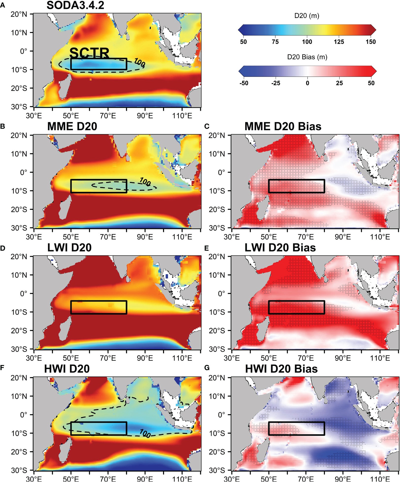
Figure 3 Spatial variation of D20 from (A) SODA3.4.2, (B) MME mean of 27 CMIP6 models, and (C) their difference/bias. (D, E) Same as (B, C) but for the models that show low Willmott index (LWI) (MRI-ESM2-0, CESM-WACCM-FV2, and FGOALS-g3). (F, G) Same as (B, C) but for the models that show high Willmott index (HWI) (GFDL-CM4, E3SM-1-0, and E3SM-1-1-ECA). The D20 bias for MME CMIP6, LWI, and HWI was calculated by subtracting the respective models from the SODA3.4.2 dataset. The hatched area indicates the D20 bias was statistically significant at a 95% confidence level based on Student’s t-test. The study period is from 1980 to 2014, and the black box denotes the SCTR region (50°E-80°E, 5°S-10°S).

Similarly, models that exhibit a positive D20 bias or LWI show a shifted and deeper thermocline depth, extending eastward across the entire Indian Ocean (Figures 3D, E). This bias exceeds the MME mean state, while a less apparent negative D20 bias is observed in the eastern Indian Ocean. On the other hand, the HWI show that the shallow thermocline extends from the SCTR region towards the east, indicating an underestimation of thermocline depth near the Sumatra coast (Figure 3F). Significant positive (negative) D20 bias is observed in the western (eastern) Indian Ocean (Figure 3G). It can be noted that the positive D20 bias in the western Indian Ocean in the MME mean is primarily contributed by models that simulate a deeper thermocline depth bias or LWI, while the negative D20 bias in the eastern Indian Ocean in the MME mean is influenced by models that better simulate D20 in the SCTR region (HWI). These interpretations of D20 bias using the MME mean are consistent with the earlier findings in Figures 1, 2.

3.2 The possible source of SCTR D20 bias in CMIP6 models from local forcing

To investigate the potential mechanisms behind the thermocline depth bias, we compared models that exhibit deeper D20 bias (LWI) with models that simulate small D20 bias (HWI) over the SCTR region. We also examined the MME mean biases, which represent the behavior of the CMIP6 models used in this study. Previous studies has indicated that upwelling in the SCTR region primarily occurs through local Ekman pumping, driven by the divergence of wind stress curl between the southeasterly trade winds in the south and westerlies in the north of the SCTR region (Xie et al., 2002; Hermes and Reason, 2008; Yokoi et al., 2008; Hermes and Reason, 2009; Schott et al., 2009). Figures 4A, B display the annual Ekman pumping velocity from ERA5 reanalysis data and the CMIP6 MME mean from 1980 to 2014, respectively. To assess the difference between the CMIP6 models and the ERA5 dataset, we calculated the Ekman pumping velocity bias and wind bias by subtracting the ERA5 values from the CMIP6 models (model minus observation). The Ekman pumping velocity bias and wind bias were averaged from 1980 to 2014 across 24 MME CMIP6 models, excluding BCC-CSM2-MR, BCC-ESM1, and CAMS-CSM1-0. The MME mean demonstrates a good reproduction of the spatial pattern of Ekman pumping velocity in both the southern and northern regions of the Indian Ocean (Figure 4B). In the south-equatorial region, approximately 5°S to 10°S, the Ekman pumping velocity shows positive values, consistent with the observations.

FIGURE 4

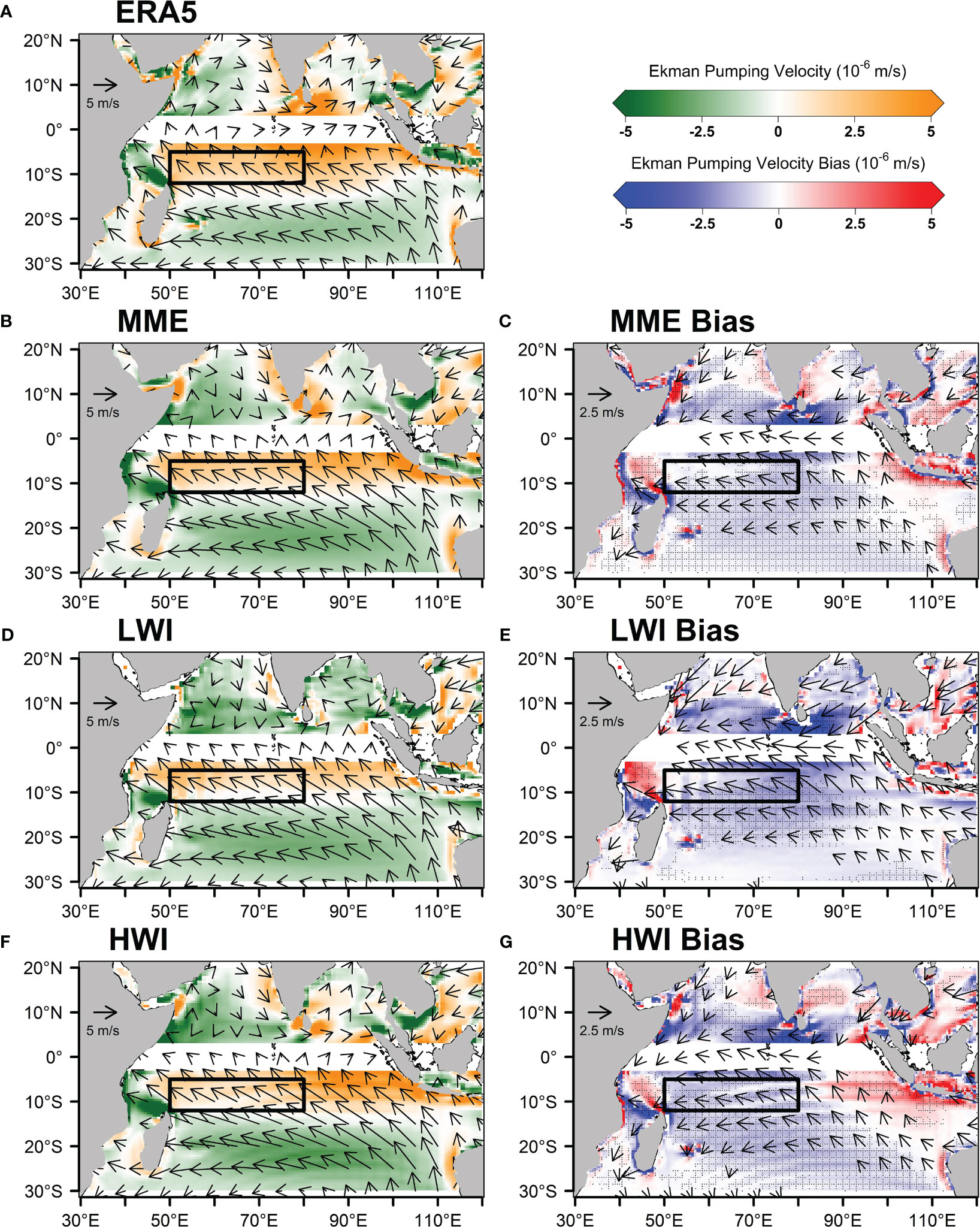
Figure 4 Annual mean of Ekman pumping velocity (color shade) and surface wind (vector) based on (A) ERA5 dataset, (B) 24 CMIP6 MME mean and (C) their difference/bias. (D, E) Same as Figure 4b and 4c but for the models that show low Willmott index (LWI) (MRI-ESM2- 0, CESM-WACCM-FV2, and FGOALS-g3). (F, G) Same as Figure 4b and 4c but for the models that show high Willmott index (HWI) (GFDL-CM4, E3SM-1-0, and E3SM-1-1-ECA). The Ekman pumping velocity and surface wind bias for MME CMIP6, LWI, and HWI were calculated by subtracting the respective models from ERA5 dataset. The hatched area indicates the Ekman pumping velocity bias was statistically significant at a 95% confidence level based on Student's t-test. The study period is from 1980 to 2014 for CMIP6, and the black box denotes the SCTR region (50oE-80oE, 5oS-10oS). Note that the wind vector scale in (B, D, F) is twice larger than in (C, E, G), and wind biases below 1 m/s have been masked out.

The CMIP6 models successfully simulate the upwelling region along the southwestern coast of Java and Sumatra. The upwelling in the southern Bay of Bengal is also captured, although it is relatively weaker compared to observations. Additionally, Figure 4C illustrates the Ekman pumping velocity bias and surface wind bias between the CMIP6 MME mean and the ERA5 dataset. In the northern Indian Ocean, the negative bias in Ekman pumping velocity varies significantly across different regions, particularly in the Arabian Sea and the southern Bay of Bengal, where northeasterly/easterly wind biases are observed. In the SCTR region, the CMIP6 models exhibit a notable negative bias in Ekman pumping velocity, particularly in the eastern part. This negative bias extends to almost the entire southern Indian Ocean, excluding the upwelling zones along the southwestern coast of Java and Sumatra and the west coast of Australia in the eastern Indian Ocean, where positive Ekman pumping velocity bias is observed. The negative bias in Ekman pumping velocity in the southern Indian Ocean is likely caused by the easterly wind bias prevalent in most parts of the Indian Ocean. Although the annual mean surface wind pattern is similar between the CMIP6 MME mean and the ERA5 data in the southern Indian Ocean, a distinct difference in surface wind direction is observed in the equatorial region, roughly between 4°N and 4°S (Figures 4A, B). The ERA5 data shows prominent westerlies in the east-equatorial region, whereas the CMIP6 models exhibit southwesterly winds. In the west-central equatorial region, the CMIP6 models show a tendency towards northward/westward movement, while southeasterly winds are observed. These discrepancies indicate the presence of easterly wind bias in the CMIP6 models (Figure 4C). The easterly wind bias is particularly pronounced in the equatorial region, leading to a reduction in the annual mean equatorial westerly winds. Additionally, it strengthens the southeasterly trade winds south of the SCTR region. The weakened equatorial westerly winds and enhanced southeasterly trade winds result in increased wind stress curl in the SCTR region (Supplementary Figure S3).

In the models with deeper D20 biases (LWI), the mean state of Ekman pumping velocity (Figure 4D) is relatively similar to that in the MME. The wind pattern in the southern Indian Ocean also shows similarities to the ERA5 dataset. However, a stronger easterly/southeasterly wind bias is present in the equatorial region, and a stronger northeasterly wind bias is observed in the northern Arabian Sea (Figure 4E). Figure 4E also demonstrates that the negative Ekman pumping velocity biases are widespread in the Indian Ocean, except in northern Madagascar. The negative Ekman pumping velocity bias in the LWI over the SCTR region is more pronounced compared to the MME mean. This stronger negative bias in Ekman pumping velocity in the LWI is attributed to the more significant easterly wind bias in the equatorial region, which is also more prominent in the LWI (Figure 4E) compared to the MME mean bias (Figure 4C). In the models with smaller D20 biases (HWI), the mean state of Ekman pumping velocity and surface wind pattern is relatively similar to observations (Figure 4F). The Ekman pumping velocity bias is smaller compared to the MME mean and LWI in the SCTR region (Figure 4G). Additionally, a relatively smaller easterly wind bias is observed in the equatorial Indian Ocean region compared to the LWI. This indicates that the models with smaller D20 biases in the SCTR region better simulate the annual mean of Ekman pumping velocity and surface wind compared to the LWI. However, negative Ekman pumping velocity and easterly wind bias still exists in the HWI. These results suggest that the negative Ekman pumping velocity bias in the CMIP6 models is likely caused by the easterly wind bias affecting the equatorial westerly wind and southeasterly trade wind in the southern Indian Ocean.

The seasonal variation of Ekman pumping velocity and the propagation of Rossby wave from the east are key factors in understanding the seasonal variability of thermocline depth (Tozuka et al., 2010; George et al., 2013; Nyadjro et al., 2017; George et al., 2018; Ma et al., 2022). In this subsection, we will focus on the role of local forcing and the role of remote forcing will be discussed in the Subsection 3.4. In order to investigate the origin of D20 biases in CMIP6 models, we analyzed the seasonal variation of Ekman pumping velocity in the SCTR region. The Ekman pumping velocity is derived from local wind and in this study, we separated it into two components: the curl term and the beta term (Tozuka et al., 2010; Yokoi et al., 2012; Nagura et al., 2013). The curl term is represented by the first term on the right-hand side of Equation (5) and largely influenced by the meridional variation of zonal wind stress (hereinafter zonal term) over the SCTR region rather than zonal variation of meridional wind stress (hereinafter meridional term) (Yokoi et al., 2008). Figure 5 shows the seasonal variation of curl term, zonal term, and meridional term and compared to observation data. The observed curl term exhibits a strong annual cycle with strong upwelling during summer and fall. The curl term also largely dominated by zonal term rather than meridional term means that the meridional gradient of zonal wind stress is more dominant than the zonal gradient of meridional wind stress (Figure 5A). In the MME (Figure 5B), the zonal term is larger compared with the observation, especially during early summer to late fall. The zonal term positive bias contributes largely to the total curl term positive bias (the respective bias was shown by red solid line in the Figure 5). In contrary, the meridional term show small negative bias with largest negative bias is in June. In the LWI (Figure 5C), the zonal term bias shows positive bias, while the meridional term bias shows negative bias. These produce positive total curl term bias throughout the year with close-to-zero bias occurred in October. In the HWI (Figure 5D), the positive bias of zonal term is the largest occurred during March and November, the largest compared with MME bias and LWI bias. The meridional term also shows negative bias, similar to the MME and LWI bias. The total curl term bias shows positive bias throughout the year except in March that shows small negative bias. According to these findings, it is evident that the bias in the curl term is predominantly influenced by the zonal term bias, resulting in a positive bias. This positive bias contributes to the enhancement of Ekman pumping.

FIGURE 5

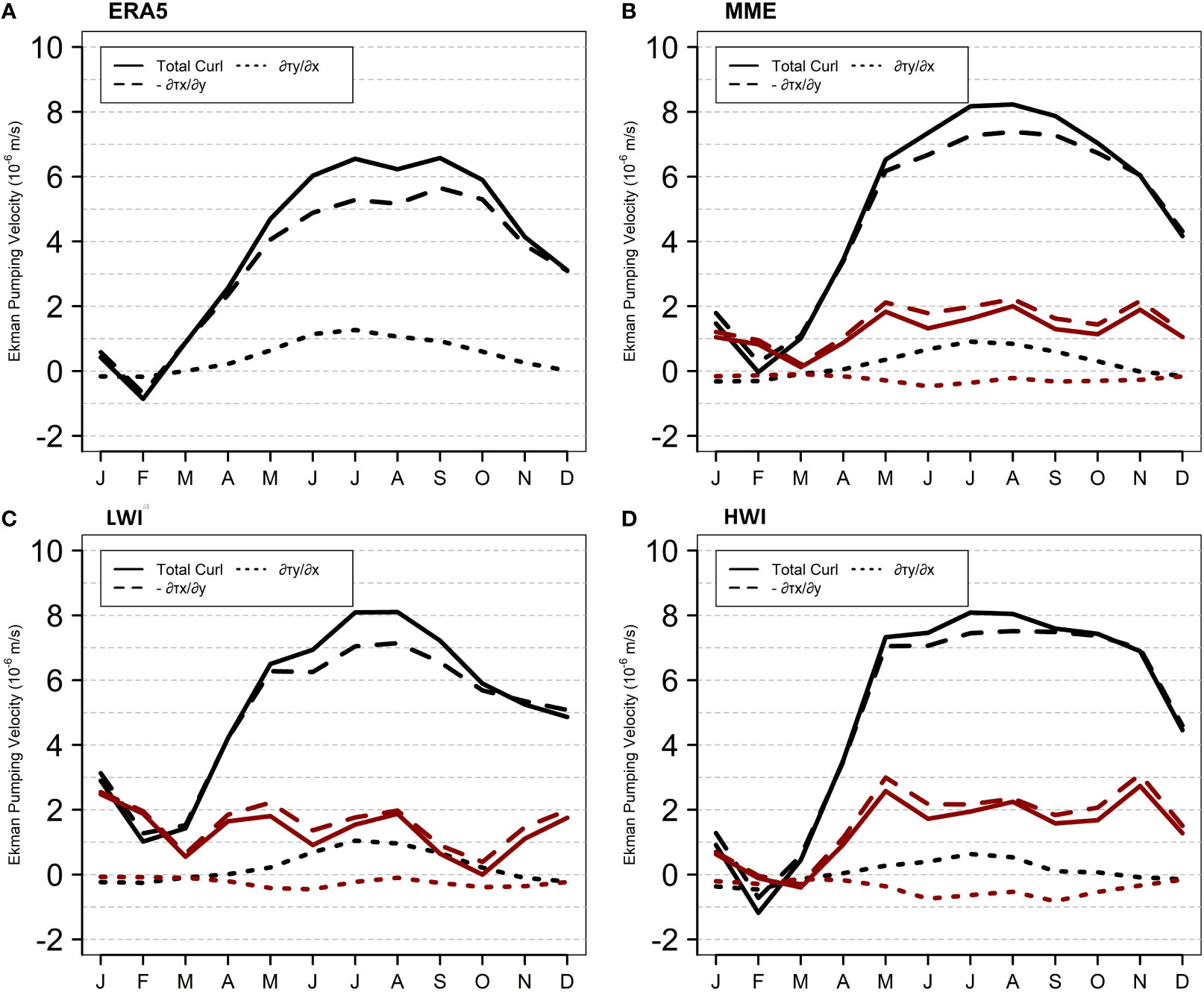
Figure 5 Monthly climatology of the curl term (solid line), zonal term ($-\frac{1}{{\rho }_{o}f}\frac{\partial {\text{τ}}_x}{\text{dy}},$ dashed line), and meridional term ($\frac{1}{{\rho }_{o}f}\frac{\partial {\text{τ}}_y}{\text{dx}}$, dotted line) for (A) the ERA5, (B) 24 CMIP6 MME mean, (C) LWI, and (D) HWI averaged over SCTR region (50°E-80°E, 5°S-10°S). Red lines in (B–D) show the difference of respective variables from the observation that was shown in (A). The period of study is from 1980 to 2014.

On the other hand, the beta term is influenced by the seasonal changes in local wind patterns associated with the Indian monsoon. It is observed from Figure 6A (dotted line) that a minimum negative beta term (downwelling) occurs in August, contributed by the summer monsoon that generates brief but stronger winds. This finding is consistent with the study by Yokoi et al. (2009), which suggests that the summer monsoon winds are intense but occur for a shorter duration, while the winter monsoon winds are weaker but last longer. In the MME of CMIP6 models (Figure 6B), the Ekman pumping velocity is underestimated from early summer in June to winter in December (shown by the negative Ekman pumping velocity bias (red solid line). The most significant deviation from observations is observed during the fall season in October, whereas relatively good agreement is found during late winter to spring with a small bias. These seasonal biases are primarily attributed to the bias in the beta term, which exhibits a larger negative bias (downwelling) compared to the positive bias (upwelling) in the curl term. In models that produce deeper D20 biases (Figure 6C), the Ekman pumping velocity is overestimated from January to May, while underestimation is observed for the remainder of the year.

FIGURE 6

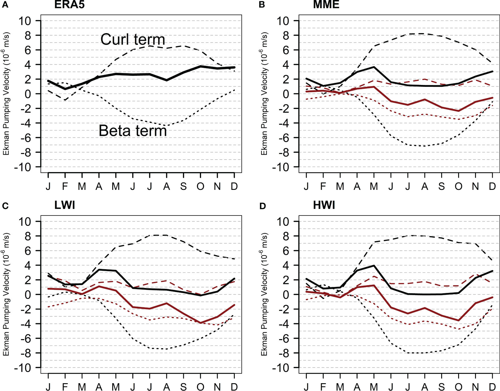
Figure 6 Monthly climatology of Ekman pumping velocity (solid line), the curl term (dashed line) and the beta term (dotted line) for (A) the ERA5, (B) 24 CMIP6 MME mean, (C) LWI, and (D) HWI averaged over SCTR region (50°E-80°E, 5°S-10°S). Red lines in (B–D) show the difference of respective variables from the observation that was shown in (A). The period of study is from 1980 to 2014.

The LWI exhibits the strongest negative bias of Ekman pumping velocity during the fall season, which might be due to an excessively large negative bias in the minimum beta term (downwelling), which suppresses the positive bias in the curl term (upwelling). The seasonal variation of Ekman pumping velocity bias in the LWI is similar to that in the MME mean because the CMIP6 models are dominated by models that simulate a negative Ekman pumping velocity bias and a positive D20 bias (deeper thermocline depth bias). In HWI (Figure 6D), the Ekman pumping velocity exhibits a similar seasonal variation compared to the LWI and MME mean. Negative biases are observed for most of the months, except in April and May. Negative biases are particularly prominent during early summer in June and July, as well as early fall in September and October. The Ekman pumping bias in LWI and HWI follows a similar seasonal pattern. However, when considering the annual mean of D20 bias, HWI exhibits smaller bias compared to LWI. This suggests that factors other than Ekman pumping contribute to the deepening of D20 bias in LWI. Another important consideration is the westward propagation of Rossby waves, which will be discussed in the Subsection 3.4.

The HWI also successfully simulates the annual cycle of the curl term, which is largely contributed by the meridional gradient of zonal wind stress and exhibits strong upwelling during the summer and fall seasons. The curl and beta terms, when analyzed separately, exhibit a strong annual cycle (Yokoi et al., 2008; Yokoi et al., 2009). However, when combined to calculate Ekman pumping velocity, a semiannual variation with two peaks per year is observed, one in spring and one in fall (Figure 5A). The SCTR region, characterized by the dominance of southeasterly trade winds in the south and the Indian monsoon in the north, leads to a nearly constant curl term from June to October (Yokoi et al., 2008; Yokoi et al., 2009). In the CMIP6, the curl term remains relatively constant for seven months, specifically from May through November, despite variations in the zonal wind stress that occurs during the summer and fall seasons (Yokoi et al., 2008). Interestingly, we find that models that simulate a shallow thermocline depth compared to observations (D20 negative bias: MPI-ESM1-2-LR, MPI-ESM1-2-HR, MPI-ESM-1-2-HAM, and CanESM5) demonstrate better performance in simulating Ekman pumping velocity or exhibit smaller biases (Supplementary Figure S4). These results indicate that the negative Ekman pumping velocity bias is significant across all models that simulate a deeper thermocline bias, with the largest bias observed during the fall season.

To further understand the negative Ekman pumping velocity bias in the SCTR region, which is likely induced by the easterly wind bias present in most of the Indian Ocean region (Figure 4), we analyze the MME mean of seasonal zonal wind bias from CMIP6 models to examine the evolution of the Ekman pumping velocity bias in the SCTR region (Figure 7). In the equatorial region, the easterly wind bias is noticeable in all months except January, February, and May. In the south of SCTR region (10°S-20°S), the wind bias is dominant from May to November. This bias is associated with the absence of westerly winds in the equatorial region. These easterly wind biases increase the meridional shear of zonal wind stress around the SCTR region and result in an increased curl term compared to observations (Figures 6B–D). However, the easterly wind biases in the southern SCTR region also enhanced the negative the beta term due to the prevalence of stronger southeasterly trade winds compared to observations (Figures 6B–D). Consequently, a prominent negative bias in the Ekman pumping velocity is observed from June to November (Figure 7), contributing to the overall weak annual mean of Ekman pumping (negative bias) (Figure 4C). This weak annual Ekman pumping is a possible cause for simulating a deeper annual mean thermocline depth in the SCTR region (Figure 3C). These results demonstrate that the CMIP6 models MME mean simulate a weak annual Ekman pumping in the SCTR region as a result of the easterly wind bias in the equatorial to the 20°S of Indian Ocean (Figures 4C; 7).

FIGURE 7

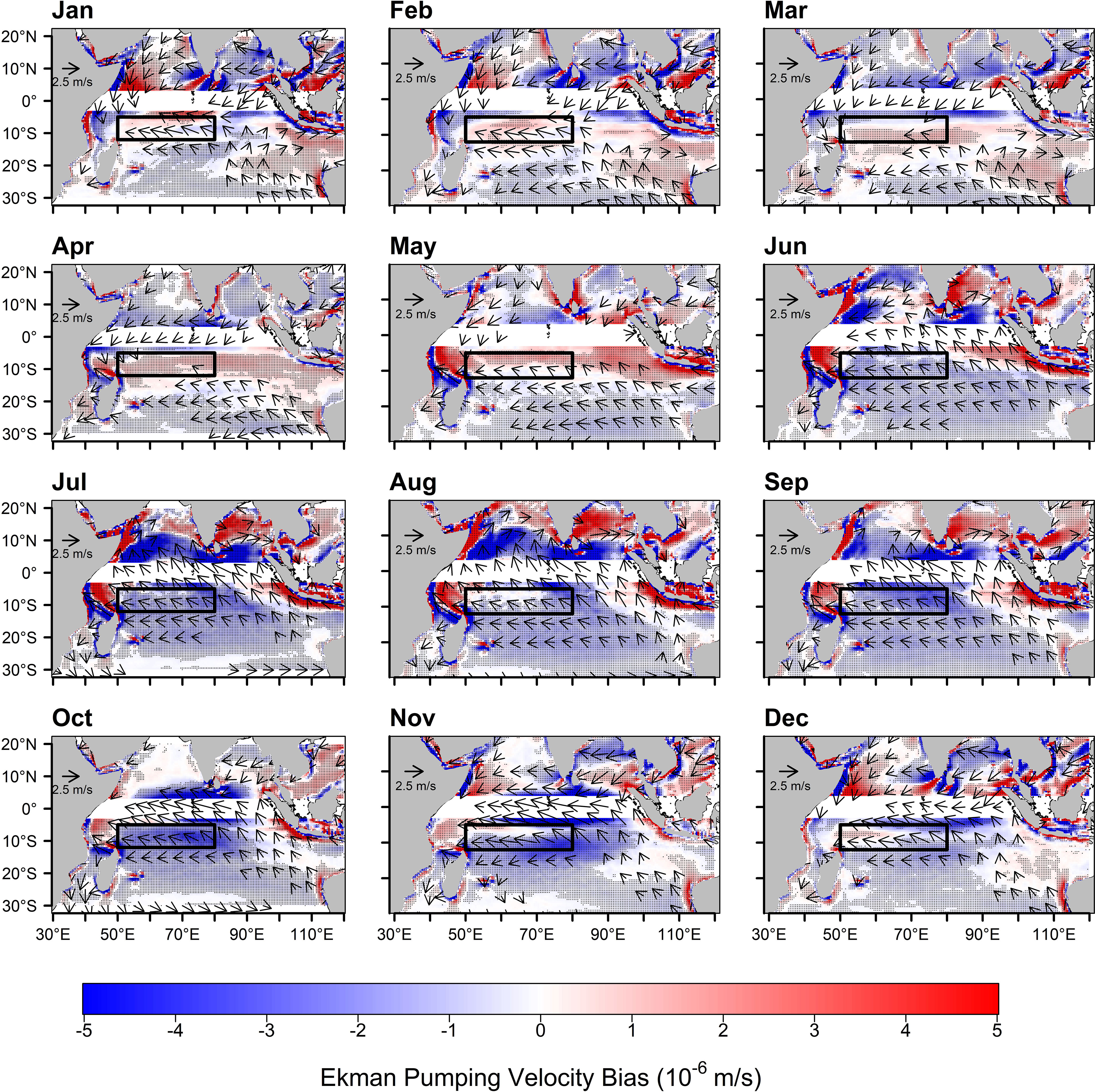
Figure 7 Monthly climatology of Ekman pumping velocity bias (color shade) and surface wind bias (vector) from MME mean of 24 CMIP6 models. Wind biases below 1 m/s have been masked out. The period of study is from 1980 to 2014 for CMIP6 models. Stippling indicates that the Ekman pumping velocity bias was significant at a 95% confidence level based on Student’s t-test.

The hypothesis that the deepening of D20 in the CMIP6 models is due to a bias in equatorial easterly winds is further supported by inter-model statistics. Figure 8A shows the connection between November-December thermocline depth and October-November Ekman pumping velocity among the CMIP6 models, which is when the negative Ekman pumping velocity bias is most significant (as indicated in Figure 6). The linear regression fitting reveals a negative correlation between thermocline depth and Ekman pumping velocity among the CMIP6 models (correlation coefficient is about -0.69 and a p-value< 0.001). This indicates that models with deeper annual mean of thermocline depth tend to exhibit weaker Ekman pumping. Additionally, Ekman pumping velocity shows a positive correlation with equatorial zonal wind in October-November (Figure 8B). Models that show westerlies or positive equatorial zonal winds are accompanied by larger positive Ekman pumping velocity in the SCTR region (correlation coefficient is around 0.85 and a p-value< 0.001). Conversely, models that show equatorial easterly winds simulate smaller Ekman pumping velocity or even negative Ekman pumping velocity (e.g. MRI-ESM2-0). Furthermore, models with positive Ekman pumping velocity (upwelling) correspond to negative wind stress curl significantly (figure not shown). The CMIP6 models also simulate larger negative wind stress curls compared to observations (Supplementary Figure S3). Equatorial zonal wind also exhibits a negative correlation with thermocline depth in the SCTR region (Figure 8C), further supporting the idea that the weaker Ekman pumping is caused by the presence of easterly wind bias in the equator, consequently deepening the thermocline depth in the SCTR region. The correlation coefficient of -0.46 in Figure 8C exceeds the 95% confidence level (p-value< 0.05).

FIGURE 8

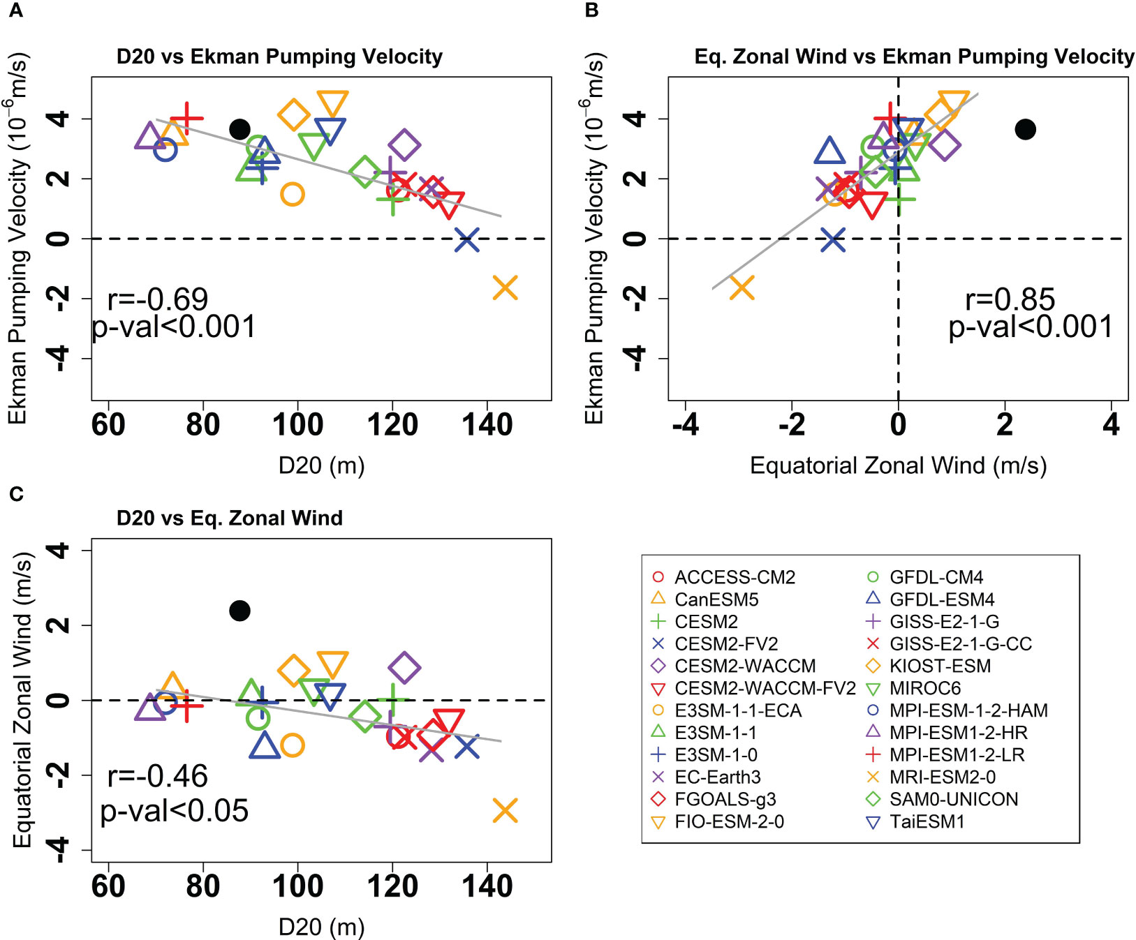
Figure 8 Scatterplot of October-November Ekman pumping velocity versus (A) November-December thermocline depth and (B) October-November equatorial zonal wind (50°E-90°E, 5°S-5°N) averaged among the 24 CMIP6 models. The scatterplot of equatorial zonal wind versus thermocline depth was also shown in (C). The Ekman pumping velocity and thermocline depth were averaged over the SCTR region (50°E-80°E, 5°S-10°S). The black dot indicates the observation from SODA3.4.2 and ERA5 dataset. The solid lines illustrate the linear regression computed by the least square method. The correlation coefficient was based on a Student’s t-test with a 95% confidence level and was shown in each panel.

3.3 The possible source of easterly wind bias: SST warm bias in the western Indian Ocean

The analysis suggests that the thermocline depth bias in the CMIP6 models is linked to the Ekman pumping velocity bias, which is in turn caused by the easterly wind bias in the Indian Ocean. To investigate the mechanism behind the easterly wind bias in the CMIP6 models, previous studies examined the CMIP5 models and proposed the possibility of an SST gradient between the western and eastern Indian Ocean as part of the IOD mode variability, which generates strong monsoon-induced equatorial easterly wind bias during the fall season (Li and Xie, 2012; Cai and Cowan, 2013; Li et al., 2015a; Li et al., 2015b; Fathrio et al., 2017). Figure 9 presents the seasonal variation of SST biases based on 27 MME CMIP6 models, overlaid with mean sea level pressure biases in the Indian Ocean region. The figure demonstrates that warmer (colder) SST biases coincide with negative (positive) sea level pressure biases, particularly in the equatorial and southern Indian Ocean. The western equatorial Indian Ocean exhibits much warmer SST biases than the eastern region, especially during the summer and fall seasons, and the warm biases extend to the middle basin from winter to spring. The difference in SST biases between the eastern and western Indian Ocean during the summer and fall is accompanied by a difference in mean sea level pressure biases. In the southern Indian Ocean, there is a positive mean sea level pressure bias throughout the year, accompanied by a dominant negative SST bias, particularly from summer to fall. In the equatorial region, a relatively warmer SST bias appears from winter to spring, accompanied by a similar negative sea level pressure bias between the east and west. Furthermore, the development of easterly (southeasterly) wind biases over the equatorial (southern) Indian Ocean from summer to fall coincides with the appearance of warmer SST bias in the western Indian Ocean. This suggests that the warmer SST bias, particularly in the western Indian Ocean, is likely to contribute to the deeper thermocline bias in the SCTR region through a stronger SST-thermocline feedback mechanism (Cai and Cowan, 2013; Li et al., 2015a). These findings support previous studies and indicate that the easterly wind bias persists in the CMIP6 models, most likely caused by the warmer SST bias in the western Indian Ocean.

FIGURE 9

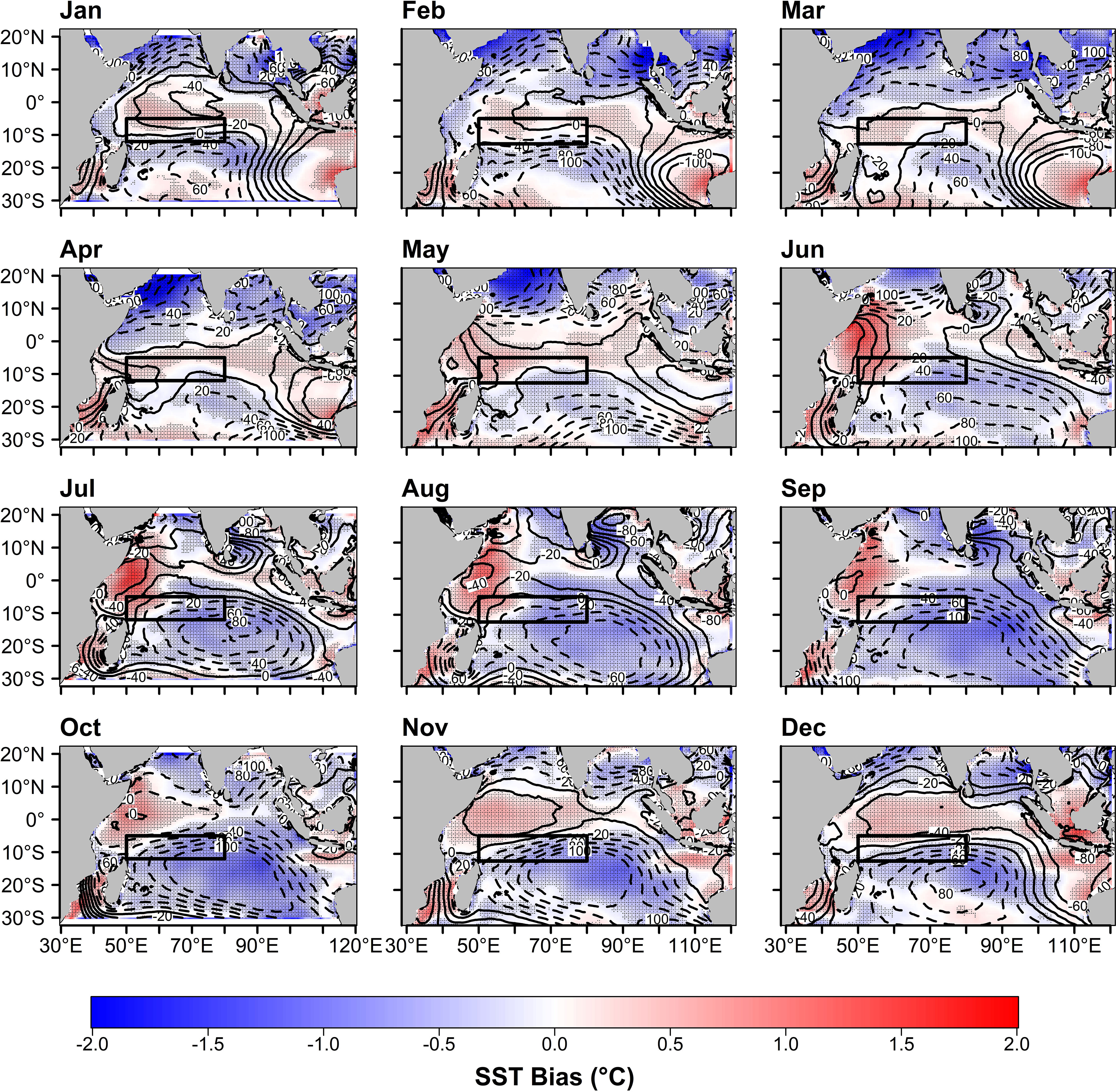
Figure 9 Monthly climatology of SST bias (colors) and mean sea level pressure bias (contours) from MME mean of 27 CMIP6 models. The contour interval for mean sea level pressure is 20 Pa and negative (positive) bias was shown by a solid (dash) line. The period of study is from 1980 to 2014 for CMIP6 models. Stippling indicates that the SST bias was significant at a 95% confidence level based on Student’s t-test. The MME mean of mean sea level pressure excluded the GFDL-CM4 model.

Inter-model statistics further support our hypothesis that the easterly wind bias in the equator originates from the difference in SST biases between the eastern and western Indian Ocean in CMIP6 models. In Figure 10A, a positive relationship is observed between the equatorial zonal wind in October-November and the east-minus-west SST difference from July-August. The models that simulate smaller positive SST difference (or even negative SST difference bias) correspond to a weakening of the zonal wind in the equator, resulting in the easterly wind bias. A significant correlation is found between equatorial zonal wind and SST difference, with a coefficient correlation is around 0.68 (p-value<0.001). Moreover, the SST difference is negatively correlated with thermocline depth, indicating that models with smaller SST differences tend to exhibit deeper thermoclines (positive D20 bias). This negative correlation is evident in Figure 10B, with a coefficient of around -0.58 (p-value<0.01). Additionally, the SST difference is positively correlated with Ekman pumping velocity (Figure 10C), suggesting that weaker SST differences correspond to weaker Ekman pumping. Therefore, the easterly wind bias induced by the SST bias difference contributes to the weakening of Ekman pumping in the SCTR region, eventually resulting in the deepening of the thermocline. Previous studies have similarly suggested that the common equatorial easterly wind bias in CMIP5 models induces excessively deep thermocline depths in the SCTR region and weakens the influence of subsurface variability on SST (Li et al., 2015a; Fathrio et al., 2017). Furthermore, the SST bias difference contributes to higher IOD peak-season amplitudes compared to observations and a slight shift towards an earlier peak in September (Cai and Cowan, 2013; McKenna et al., 2020).

FIGURE 10

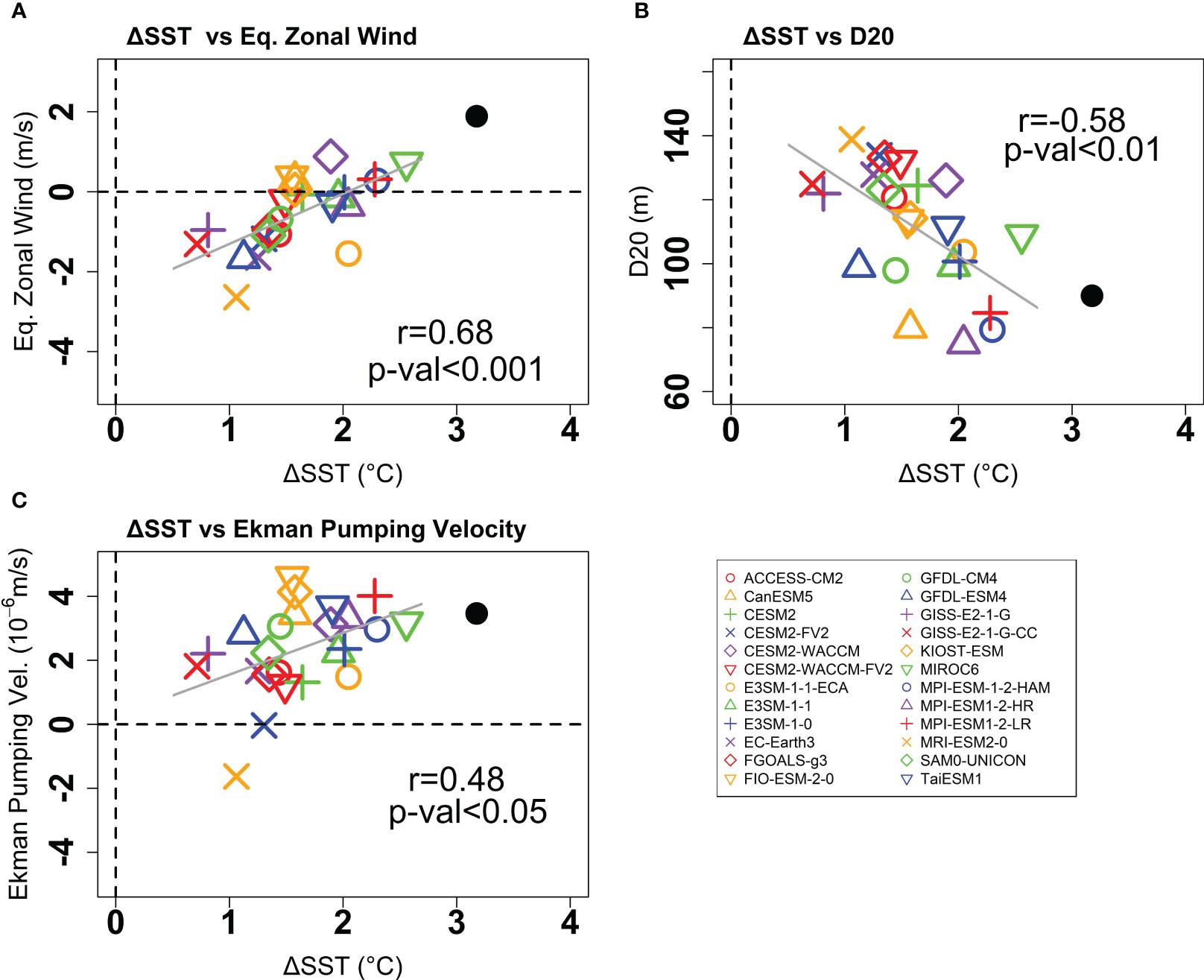
Figure 10 Scatterplot of east-minus-west SST in July-August versus (A) October-November equatorial zonal wind (50°E-90°E, 5°S-5°N), (B) November-December thermocline depth, and (C) October-November Ekman pumping velocity averaged among the 24 CMIP6 models. The western and eastern Indian Ocean was defined by 50°E-55°E and 90°E-95°E in the band of 10°S-10°N latitudes, respectively. The Ekman pumping velocity and thermocline depth were averaged over the SCTR region (50°E-80°E, 5°S-10°S). The black dot indicates the observation from SODA3.4.2 and ERA5 dataset. The solid lines illustrate the linear regression computed by the least square method. The correlation coefficient was based on a Student’s t-test with a 95% confidence level and was shown in each panel.

Although our study does not specifically focus on the source of the SST warming bias in the western Indian Ocean, we explore possible explanations based on previous research. Fathrio et al. (2017) conducted a study using 21 historical runs of CMIP5 models and proposed that the warmer SST biases in the MME CMIP5 models in the western Indian Ocean could be attributed to the advection of warm water by the East African Coastal Current (EACC). Based on their findings, we calculate the temperature advection caused by the surface ocean current using data from 25 available CMIP6 models (excluding GFDL-ESM4 and MIROC6). This analysis aims to provide insights into the potential mechanisms contributing to the simulated SST warming bias in the western Indian Ocean. The advection term can be decomposed into the zonal advection term and meridional advection term (Ng et al., 2015; Fathrio et al., 2017) as follows:

$\begin{array}{ll}-{\mathit{\text{V}}}_H·\mathbf{\nabla }{T}_H=-\left(u\frac{\partial T}{\partial x}+v\frac{\partial T}{\partial y}\right)& (6)\end{array}$

where the subscript H indicates the horizontal direction of SST (T) and ocean current (V) consisting of the zonal and meridional current u and v respectively. Figure 11 presents the scatter plot between the August-September SST bias in the western Indian Ocean to the temperature advection term. The correlation analysis reveals a positive relationship between the horizontal advection term in June-July and the western Indian Ocean SST bias in August-September (Figure 11A). This indicates that models exhibiting a positive SST bias tend to simulate a more pronounced horizontal advection term. Although the correlation coefficient falls outside the significance level, it is noteworthy that the positive association suggests that the warming SST bias could be attributed to a weakened negative horizontal advection term, indicating a cooling tendency.

FIGURE 11

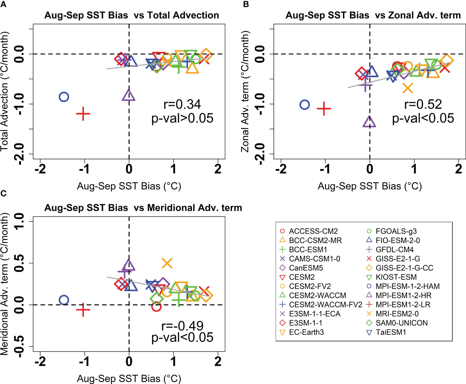
Figure 11 Scatterplot of August-September SST bias averaged over the western equatorial Indian Ocean (45°E-60°E, 10°S-10°N) among the CMIP6 models used in this study (excluding E3SM-1-0, GFDL-ESM4, and MIROC6) versus (A) temperature tendency due to horizontal advection (total advection), (B) zonal advection term, and (C) meridional advection term. The regression computations exclude two outliers: MPI-ESM-1-2-HAM and MPI-ESM1-2-LR. The solid lines illustrate the linear regression computed by the least square method. The correlation coefficient was based on a Student’s t-test with.

Moreover, the positive correlation between SST bias and the SST tendency is predominantly driven by the zonal advection term (Figure 11B). This implies that the mechanisms contributing to the warm SST bias during August-September in the western equatorial Indian Ocean involve the presence of zonal advection, with relatively warm SST biases transported over the central equatorial Indian Ocean by anomalous westward surface currents. Additionally, the EACC, flowing northeastward, facilitates the horizontal transport of relatively warm SST biases across the southwestern equatorial Indian Ocean (Schott and McCreary, 2001; Schott et al., 2009; Fathrio et al., 2017). It is worth noting that a segment of the EACC transports somewhat warm SST biases towards the Arabian Sea (Fathrio et al., 2017), leading to a negative correlation in the north-south transport of SST biases (Figure 11C). These findings point to potential mechanisms that contribute to the warm SST bias in the western equatorial Indian Ocean during the summer to fall period, partially attributed to the influence of the ocean current system.

3.4 The role of remote forcing: westward propagating Rossby wave during IOD events

The interannual variability of the SCTR in the southwestern Indian Ocean is significantly influenced by the presence of Rossby waves originating from the east, particularly during El Niño-Southern Oscillation (ENSO) and IOD events (Masumoto and Meyers, 1998; Xie et al., 2002; Nyadjro et al., 2017; Chen et al., 2022; Lee et al., 2022). For the sake of convenience, we focus solely on IOD events and compute the composite of the D20 anomaly based on both positive and negative IOD occurrences. The IOD is one of the prominent climate teleconnection patterns in the Indian Ocean, exerting considerable influence on climate variability in surrounding regions (Saji et al., 1999; Jayakumar and Gnanaseelan, 2012; Ng et al., 2014; Ng et al., 2015; Nyadjro et al., 2017; Phillips et al., 2021; Mubarrok and Jang, 2022; Sajidh and Chatterjee, 2023). In this subsection, we investigate the role of westward-propagating Rossby waves during positive and negative IOD events in the CMIP6 models, comparing them with observed data. We determine positive and negative IOD phases using the Dipole Mode Index (DMI), which measures the anomalous SST gradient between the western equatorial Indian Ocean (50°E-70°E and 10°S-10°N) and the southeastern equatorial Indian Ocean (90°E-110°E and 10°S-0°N). In this study, we define the positive (negative) IOD phase when the DMI exceeds (falls below) 0.5°C for at least of three months. Composite means of variables during IOD event years are denoted as year (0), while those in the years immediately following the event are labeled as year (+1). Noted that the occurrence of positive and negative IOD events in the CMIP6 models does not align with those observed in observation. As a result, we have chosen to select only the 5 corresponding years with the highest (lowest) values of positive (negative) DMI for each CMIP6 model in order to calculate composites for positive (negative) IOD events.

Figure 12 show the composite mean of D20 anomalies during positive IOD events. During positive IOD events, the observed positive D20 anomaly initially appears around 90°E in September (0). These positive D20 anomalies then propagate westward to the SCTR region and reach their peak from November (0) to January (+1) around 75°E. The deepened D20 anomalies persist in the western part of the SCTR until the end of the year (+1) (Figure 12A). The initiation of westward propagating Rossby wave is related to the anomalous easterly winds that are observed in the southeastern tropical Indian Ocean during July (0) (Supplementary Figure S5A). These easterly wind anomalies peak during September (0) to November (0) in the SCTR region, lead to anticyclonic wind stress curl and associated to negative Ekman pumping anomalies (downwelling) (Supplementary Figure S6A), resulting in the deepening of the thermocline east of SCTR region and further propagate to the SCTR region. These results are consistent with previous studies of Lee et al. (2022) and Nyadjro et al. (2017).

FIGURE 12

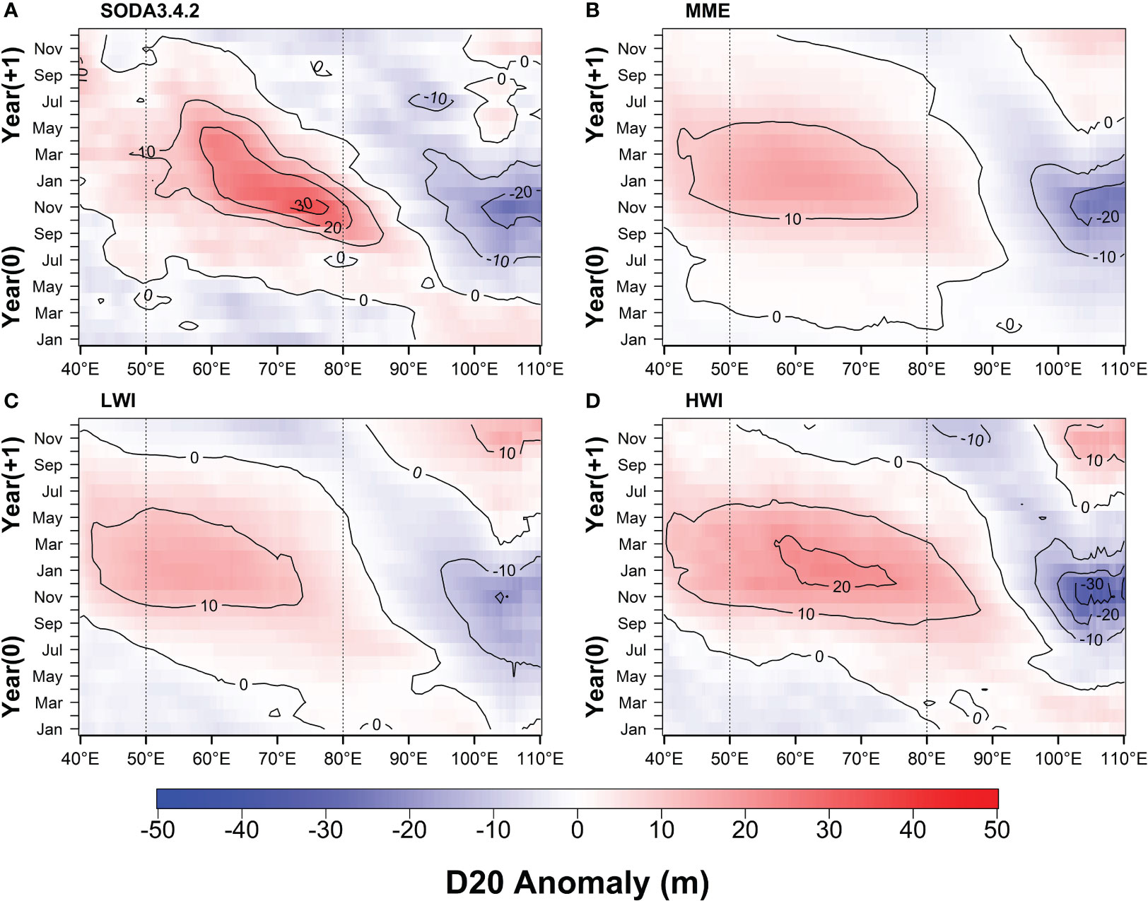
Figure 12 Composite means of D20 anomalies during IOD positive events based on (A) SODA3.4.2, (B) 27 MME CMIP6 models, (C) LWI, and (D) HWI averaged over 5°S-10°S latitudinal band. The positive events were classified using Dipole Mode Index (DMI), the anomalous SST gradient between the western equatorial Indian Ocean (50oE-70oE and 10oS-10oN) and the southeastern equatorial Indian Ocean (90°E-110°E and 10°S-0°N). The IOD events during the period of 1980−2014 based on DMI were used. The climatology used to compute the monthly anomalies represents the 1980−2014 base period. The positive IOD events are characterized by a positive DMI, larger than or equal to +0.5°C. IOD event years (year 0) and the year following the IOD events (year +1) are shown. Composite calculations were based on the five strongest positive IOD events.

In the CMIP6 models, the D20 anomalies are smaller compared to the D20 anomalies from SODA3.4.2, and this pattern is observed in both the MME mean, LWI, and HWI models. The positive D20 anomalies range from approximately 10 to 20 m in the CMIP6 models, while in SODA3.4.2, they can reach up to 30 m. The D20 anomalies (around 10 m) begin to appear around 75°E in November (0) in the MME (Figure 12B) and LWI (Figure 12C) and propagate westward through the SCTR region, reaching the western Indian Ocean (around 40°E) by May of the following year (+1). In the LWI models (Figure 12D), the D20 anomalies start to emerge east of the SCTR (around 90°E) in November (0) and gradually propagate into the SCTR region by January of the following year (+1). The D20 anomalies peak during December (0) to March (+1) around 65°E, which is slightly shifted westward compared to the observed D20 anomalies peak location. The speed of the propagation of positive D20 anomalies in the CMIP6 models is approximately 0.15 m/s for MME, 0.18 m/s for LWI, and 0.20 m/s for HWI, while it is about 0.12 m/s in SODA 3.4.2. The smaller amplitude of positive D20 anomalies is likely correlated with the weakened positive wind stress curl in the eastern Indian Ocean (Supplementary Figure S5B). During November (0), the wind stress was predominantly northeasterly around 90°E and extended to 60°E. This weakened positive curl is also associated with the reduction in negative Ekman pumping (Supplementary Figure S6B), contributing to the smaller-amplitude positive D20 anomalies compared to observations. These patterns of wind stress curl and Ekman pumping were relatively similar among MME, LWI, and HWI, although LWI extended further to the western side of SCTR.

Figure 13 illustrates the composite mean of D20 anomalies during negative IOD events. These events typically begin with the emergence of negative D20 anomalies around 90°E in June (0). Subsequently, these negative D20 anomalies propagate westward and peak from November (0) to January (+1) around 75°E. The shallow D20 anomalies persist in the western part of the SCTR until May to June of the following year (+1) (Figure 13A). The initiation of westward-propagating Rossby waves is closely linked to anomalous westerly winds observed in the southeastern tropical Indian Ocean during July (0) (Supplementary Figure S7A). These westerly wind anomalies reach their peak from September (0) to November (0), resulting in negative wind stress curl anomaly and positive Ekman pumping anomalies (upwelling) (Supplementary Figure S8A). These atmospheric conditions lead to the shallowing of the thermocline east of the SCTR region, further propagating westward into the SCTR region.

FIGURE 13

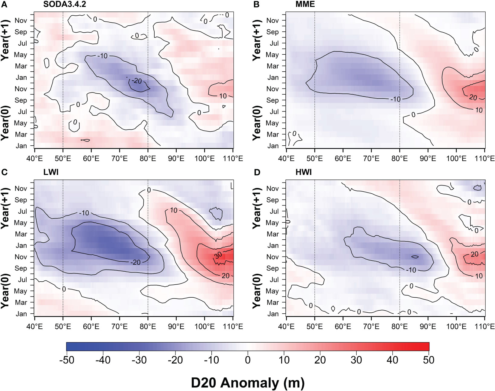
Figure 13 Composite means of D20 anomalies during IOD negative events based on (A) SODA3.4.2, (B) 27 MME CMIP6 models, (C) LWI, and (D) HWI averaged over 5°S-10°S latitudinal band. The negative events were classified using Dipole Mode Index (DMI), the anomalous SST gradient between the western equatorial Indian Ocean (50oE-70oE and 10oS-10oN) and the southeastern equatorial Indian Ocean (90°E-110°E and 10°S-0°N). The IOD events during the period of 1980−2014 based on DMI were used. The climatology used to compute the monthly anomalies represents the 1980−2014 base period. The negative IOD events are characterized by a negative DMI, smaller than or equal to −0.5°C. IOD event years (year 0) and the year following the IOD events (year +1) are shown. Composite calculations were based on the five strongest negative IOD events.

The negative D20 anomalies from CMIP6 models exhibit smaller magnitudes when compared to the D20 anomalies observed in SODA3.4.2 for the MME mean and HWI models. The negative D20 anomalies in the MME mean and HWI models is approximately -10 m, whereas in SODA3.4.2, it can reach depths of up to -20 m. The negative D20 anomalies in LWI is larger compared to the MME and HWI (~ -20 m) and extend to the western SCTR in the May (+1). The onset of D20 anomalies (approximately -10 m) is observed around 85°E in both the MME (Figure 13B) and LWI (Figure 13C) models during September (0). These anomalies then propagate westward through the SCTR region, reaching the western Indian Ocean (around 50°E) by May of the subsequent year (+1). In the HWI models (Figure 13D), the emergence of D20 anomalies initiates to the east of the SCTR (around 90°E) in September (0) and gradually progresses into the SCTR region (around 60°E) by March of the following year (+1). The peak of D20 anomalies occurs during the period from December (0) to March (+1) around 65°E, with a slight westward shift compared to the observed peak locations.

The speed of propagation of negative D20 anomalies in the CMIP6 models is estimated to be around 0.21 m/s for MME, 0.16 m/s for LWI, and 0.22 m/s for HWI, whereas it measures approximately 0.11 m/s in SODA 3.4.2. The reduced amplitude of negative D20 anomalies in the CMIP6 models is likely associated with existence of wind stress curl in the eastern Indian Ocean (Supplementary Figure S7B). Specifically, in August (0) to November (0), the wind stress is predominantly southwesterly around 90°E, extending to 70°E. This weakened negative curl is further correlated with a decrease in positive Ekman pumping (Supplementary Figure S8B), contributing to the smaller amplitudes of negative D20 anomalies compared to the observations. These patterns of wind stress curl exhibit relative similarity among MME, LWI, and HWI, although LWI extends further to the eastern side of the SCTR (60°E). The Ekman pumping patterns also show a positive bias around 90°E in the July (0) and reach to the 50°E and 60°E for LWI and MME, respectively, in the November (0).

To characterize the westward propagating Rossby wave patterns in the CMIP6 models, we computed the skewness of D20 anomalies and SST anomalies spatially averaged over the SCTR region (Supplementary Figure S11). In the observations, the D20 anomalies exhibited positive skewness, indicating that the SCTR region were predominantly influenced by positive anomalies, likely associated with positive IOD events. This aligns with the earlier findings in Figures 12A; 13A, which showed that observed positive D20 anomalies during positive IOD events had larger amplitudes compared to observed negative D20 anomalies during negative IOD events. However, in contrast to the observations, most CMIP6 models displayed smaller skewness and were characterized by negative skewness (20 out of 27 models) (Supplementary Figure S11A). This implies that in the CMIP6 models, D20 anomalies were primarily driven by negative anomalies rather than positive ones. Additionally, we examined the skewness of SST anomalies as shown in Supplementary Figure S11B. In the observations, SST anomalies exhibited positive skewness, indicating that warm anomalies in the SCTR region were more pronounced than cold anomalies. This pattern may be attributed to strong positive IOD events, which are indicated by warm SST anomalies in the western Indian Ocean compared to cold SST anomalies during negative IOD events, driven by the asymmetry of the positive Bjerknes feedback mechanism (Ng et al., 2014; Ng and Cai, 2016; McKenna et al., 2020; An et al., 2023). In contrast, in the CMIP6 models, the majority of models showed negative skewness in SST bias (23 out of 27 models). This suggests that the distribution of SST anomalies in these models was largely influenced by contributions from cold SST anomalies rather than warm ones. This finding is consistent with Supplementary Figure S11A, which indicated that skewness of D20 anomalies in the CMIP6 models were also predominantly influenced by negative D20 anomalies (associated with upwelling), resulting in the prevalence of cold SST anomalies.

4 Discussion

Previous studies have demonstrated that the SCTR is primarily influenced by local Ekman pumping velocity, driven by a combination of southeasterly trade winds and westerly winds near the equator, resulting in a negative wind stress curl (Xie et al., 2002; Hermes and Reason, 2008; Yokoi et al., 2008). The climate teleconnection patterns, such as IOD, also can trigger oceanic Rossby wave from the east and travel westward, controlling the interannual variability in the SCTR region (Xie et al., 2002; Schott et al., 2009; Jayakumar and Gnanaseelan, 2012; Ma et al., 2022). Due to its shallow thermocline depth, the SCTR region is known for strong sea-air interaction (Klein et al., 1999; Tozuka et al., 2010) and is considered a crucial area for IOD prediction (Luo et al., 2008). Additionally, previous studies utilizing observational and reanalysis data have emphasized the SCTR region is essential in shaping climate variations in the Indian Ocean (McPhaden et al., 2009; Vailard et al., 2009). While attempts have been made to assess the dynamics of the SCTR region using available CGCMs, it has been observed that these models still inadequately simulate the SCTR dynamics. Consequently, improving the simulation of the SCTR region in state-of-the-art CGCMs has become crucial. In this study, our aim is to evaluate the capability of CMIP6 models in simulating the thermocline depth and its variability over the SCTR region by comparing them with observational data. By analyzing output from the CMIP6 models, we have investigated potential factors contributing to the thermocline depth variations in the SCTR region in the southwestern Indian Ocean.

Similar to the findings of Yokoi et al. (2009) and Li et al. (2015a), our analysis reveals that the CMIP6 models simulate a deeper thermocline depth in the SCTR region compared to observations. The Ekman pumping over the SCTR region is weaker in the CMIP6 models than in the observational data. The largest bias in Ekman pumping velocity occurs during the fall season and is primarily driven by the beta term, which is proportional to the strength in zonal wind stress bias above the SCTR region. Notably, the CMIP6 models exhibit a significant easterly wind bias in the equatorial and southern Indian Ocean during summer and fall. This easterly wind bias likely contributes to the strengthening of the curl term, which is largely proportional to the meridional changes in zonal wind stress (resulting in upwelling and a positive bias in Ekman pumping velocity). However, the easterly wind bias also reinforces the negative beta term (resulting in downwelling and a negative bias in Ekman pumping velocity), which surpasses the curl term and leads to an overall negative bias in the total Ekman pumping velocity (smaller than observed). The easterly wind bias is likely induced by the SST difference (east-minus-west) between the eastern and western Indian Ocean, with positive (negative) SST biases present over the western (eastern) Indian Ocean, consequently reducing the SST difference compared to observations.

Specifically, the positive SST bias observed over the western Indian Ocean is likely a result of the horizontal transport of relatively warm SST biases by ocean currents across the southwestern equatorial Indian Ocean, facilitated by the EACC. This finding is consistent with the results of Fathrio et al. (2017), which emphasized the significance of ocean currents in the development of SST biases in the western equatorial Indian Ocean. Additionally, the warm SST bias in the western Indian Ocean may be attributed to the weakened South Asian summer monsoon in the western basin during summer, as highlighted by Boos and Hurley (2013); Li et al. (2015b), and Li and Xie (2012). The CMIP5 models indicate that the southwest summer monsoon is too weak over the Arabian Sea, leading to a warm SST bias in the western equatorial Indian Ocean (Li et al., 2015a). During fall, the Bjerknes feedback mechanism intensifies the SST biases, resulting in an IOD-like pattern accompanied by easterly wind bias and a pronounced eastward shoaling of the thermocline depth over the equatorial Indian Ocean (Li et al., 2015a). Our findings demonstrate that the eastward shoaling is evident in most of the CMIP6 models examined in this study (Figure 2B), and the thermocline depth bias exhibits shallower (deeper) depths in the eastern (western) Indian Ocean (Figure 3C), supporting the earlier conclusions of Li et al. (2015a). Moreover, we observed a shift in the SCTR thermocline dome towards the east. This eastward displacement of the dome is likely a consequence of the eastward shoaling thermocline depth in most of the CMIP6 models (Wang et al., 2021). This phenomenon has been documented in previous research, such as Nagura et al. (2013), who demonstrated that the eastward migration of the thermocline dome in the CMIP5 models can be primarily attributed to prominent easterly biases along the equator during boreal summer and fall, consistent with the results made in the present study. These easterly biases, particularly notable near the equator, lead to shallower thermocline biases along the Java and Sumatra coasts through Kelvin wave dynamics and create a spurious upwelling dome in the region. Although further study is required to see the Kelvin wave dynamic in the CMIP6 models, this mechanism likely contributes to the eastward shift in the SCTR thermocline dome observed in the CMIP6 models. These results indicate that the bias associated with the wind system in the CMIP5 models appears to persist as an unresolved issue in the CMIP6 models.

Several studies have emphasized the significance of the curl term and beta term in the Ekman pumping velocity, which contribute to the formation of shallow thermocline depths in CMIP models (Yokoi et al., 2009; Nagura et al., 2013). In this study, we observed that the easterly wind bias amplifies the meridional shear of zonal wind stress, thereby intensifying the positive curl term. This finding differs from the conclusions of Nagura et al. (2013), who discussed a reduction in the curl term due to a decrease in meridional shear of zonal wind stress caused by easterly wind bias. This apparent contradiction can be attributed to two reasons. Firstly, our study defines the SCTR region as located from 50°E to 80°E and from 5°S to 10°S, whereas Nagura et al. (2013) focused on a slightly different geographical range, ranging from 60°E to 90°E and from 5°S to 12°S. This variation in the chosen study area boundaries can impact the sensitivity of thermocline depth variability observed. Furthermore, previous studies, such as those conducted by Praveen Kumar et al. (2014) and Trenary and Han (2012), have indicated that the semi-annual variability in this region significantly increases to the west of 70–80°E and north of 10°S. Conversely, in the southern part of the region, specifically between 8°S and 12°S, the dominant pattern is characterized by an annual cycle. These regional variations underscore the importance of defining the specific boundaries when studying the SCTR region’s thermocline depth variability. Secondly, our findings indicate a prominent easterly wind bias during summer to fall, extending from the equator to around 15°S in the southern part of the SCTR region. In contrast, Nagura et al. (2013) highlighted the existence of a westerly wind bias at 15°S latitude. This discrepancy possibly reflects differences in the characteristics of easterly wind bias between CMIP5 and CMIP6 models, which could serve as an intriguing topic for future research. Nevertheless, our present study demonstrates that the beta term counteracts the curl term, leading to a negative bias in the Ekman pumping velocity. Consequently, this deepens the thermocline depth in the SCTR region, supporting with the findings of previous studies.

This study identifies the existence of the positive bias in thermocline depth in the SCTR region of the southwestern tropical Indian Ocean in CMIP6 models, which is consistent with previous generations of CMIPs, namely CMIP3 (Yokoi et al., 2009) and CMIP5 (Nagura et al., 2013; Zheng et al., 2016). To provide a brief comparison, we also calculated the D20 bias for 25 CMIP5 models, as portrayed in Supplementary Figure S9. Similar to CMIP6 models, the previous CMIP5 models also exhibit an overestimation of thermocline depth compared to observations, with 22 out of 25 models showing positive biases. However, in contrast to the CMIP6 models that generally exhibit positive thermocline biases across the entire Indian Ocean region, the spatial variation of D20 bias in CMIP5 models differs from model to model. For example, some CMIP5 models demonstrate strong negative biases in the southern part of the Indian Ocean, near the latitude of 30°S (e.g., CSIRO-Mk3-6-0, IPSL-CM5A, MIROC-ESM). This negative bias in thermocline depth is also evident in some CMIP6 models, such as MPI-ESM-1-2-HAM, MPI-ESM1-2-LR, FIO-ESM-2-0, and SAM0-UNICON (Figure 1). The shallower-than-observed D20 in the Southern Ocean is likely caused by the overestimation of westerly wind simulation in CMIP6 climate models (Goyal et al., 2021; Deng et al., 2022), which potentially induces relatively larger Ekman pumping velocities and consequently shallows the thermocline depth. Another notable D20 bias is observed in the northern Indian Ocean, particularly in the Arabian Sea, for both CMIP5 (e.g., CanESM2, CCSM4, GFDL-ESM2M) and CMIP6 models (e.g., CESM2, FGOALS-g3, KIOST-ESM) that show an overestimation of D20 bias. Furthermore, the MME mean of D20 bias in CMIP6 models is slightly deeper compared to CMIP5 models (Supplementary Figure S10). The Welch’s two-sample t-test indicates that the mean D20 bias does not exhibit a statistically significant difference between CMIP6 and CMIP5 (p-value=0.83). However, the inter-model variability, as measured by the MME standard deviation of D20 bias in CMIP models, is smaller in CMIP6 models compared to CMIP5 models (with standard deviations of approximately 18.81 m and 20.77 m, respectively). These findings suggest that although CMIP6 models have shown improved inter-model variability in D20 bias, they are not substantially better in simulating thermocline depth compared to CMIP5 models.

In this study, we focus on examining the bias in thermocline depth attributed to local forcing, particularly the bias in Ekman pumping velocity driven by easterly wind bias. It is worth noting that the variability observed in the SCTR region may also be subject to remote forcing factors. For instance, the propagation of westward Rossby waves could play a significant role in influencing the SCTR region’s characteristics. We observed that the propagation of D20 anomalies during IOD events in the CMIP6 models is relatively limited compared to what is seen in observations. Additionally, the Rossby waves in the models tend to travel at a faster speed from the eastern to the western Indian Ocean. Li et al. (2015a) identified the westward-propagating downwelling Rossby wave in the southern Indian Ocean as a significant factor contributing to the excessively deep thermocline depth bias over the SCTR region in CMIP5 models. The Rossby wave in the tropical southern Indian Ocean was induced by easterly wind bias in the equatorial region, similar to the equatorial easterly wind anomalies during El Niño that induce a southern Indian Ocean Rossby wave. The present study reveals that the persistent equatorial easterly wind bias in CMIP6 models is a primary factor driving the excessively deep thermocline depth bias. However, our study demonstrates that the influence of Rossby waves on thermocline depth bias is not as significant as the local forcing caused by Ekman pumping induced by local winds, even though the CMIP6 models can successfully reproduce the eastward propagation of Rossby waves. The time-longitude section of thermocline depth bias reveals that the positive bias predominantly occurs during the winter season in the region around 50°E to 80°E, rather than originating from the eastern part (Supplementary Figure S12). There is also a possibility that the signal of the Rossby wave from the east has been mixed by its interaction with the local processes (Xie et al., 2002; Hermes and Reason, 2008). Additionally, the westward-propagating downwelling (upwelling) Rossby waves originating from the east during positive (negative) IOD events play a role in the surface layer, inducing warm (cool) SST anomalies (Ng et al., 2015). In observations, the SST warming in the western part during positive IOD events is more pronounced compared to the SST cooling during negative IOD events (indicated by positive SST anomaly skewness and positive D20 anomaly skewness). However, in most CMIP6 models, we observe negative SST anomaly skewness and negative D20 anomaly skewness. One plausible explanation for this is the significant influence of the nonlinear positive Bjerknes feedback on D20 anomalies and SST anomaly skewness. During positive IOD events, the thermocline-induced warming is relatively weak. This is because, in response to anomalous easterlies, further deepening of the already deep climatological mean thermocline depth has little impact on surface SST. Consequently, a deep mean thermocline allows cold SST anomalies to develop more strongly, while the growth of warm SST anomalies is weaker. These conditions result in negative skewness of SST anomalies, indicating that the cold SST anomaly signal is more prominent in the context of the warmer climatological mean SST (Ng et al., 2014; Ng and Cai, 2016).

In addition, the configuration of individual models, such as vertical mixing schemes (Yuchao et al., 2020) and spatio-temporal resolutions (Nagura et al., 2013), used in this study may have influenced the magnitude of thermocline depth bias in the CMIP6 models. Previous study by Feng et al. (2023) showed that, in addition to the easterly wind bias, the vertical mixing and vertical shear in current was contributed to the subsurface temperature bias in the tropical Indian Ocean. The increasing trend in the freshwater flux in the CMIP6 models contributes to the more stable stratification, decreasing the vertical mixing between mixed layer and deeper layer and, consequently, inducing a warming bias in SST (Ke-xin and Fei, 2022). Furthermore, previous research by Nagura et al. (2013) indicated that the spatial resolution of CMIP5 models is not a crucial factor in simulating the thermocline depth. Additionally, they found that model parameterizations, such as atmospheric convection schemes and ocean-mixed layer schemes, have less impact on the simulation of thermocline depth. However, in the present study, a simple correlation analysis reveals some interesting findings. There is a negative relationship between the zonal resolutions of the individual models used in this study (Table 1) and the thermocline depth bias, with a correlation coefficient of approximately -0.33 and a p-value of around 0.086. This indicates that at a 90% confidence level, models with higher zonal resolutions tend to produce smaller thermocline depth biases. Conversely, when considering the meridional resolutions of the models, there is no significant correlation with the thermocline depth bias, as evidenced by a correlation coefficient of around 0.01 and a p-value of approximately 0.93. These results suggest that the zonal resolution plays a more critical role in shaping the thermocline depth than the meridional resolution. Considering the significance of accurately simulating the SCTR region, these findings imply the need for future improvements in model configuration, particularly with regards to enhancing spatial resolution, to capture the characteristics of the thermocline depth better.

5 Conclusions

This study analyzes the thermocline depth bias over the SCTR region by focusing on the influence of local forcing in the 27 CMIP6 models. Similar to the previous generation of CMIP models, the CMIP6 models show that the thermocline depth over the SCTR region is considerably deeper compared to observations. Of the 27 CMIP6 models analyzed, 23 models reproduce a deeper thermocline depth. This deep bias is probably caused by the weakening of the Ekman pumping in the SCTR region. The easterly wind bias is pronounced in the equator to the southern Indian Ocean around 20°S, weakening the westerly wind at the equator and strengthening the southeasterly trade wind in the southern SCTR region. The combination of these wind systems affects the two components of the Ekman pumping velocity, the curl term and the beta term. In the models that produce deeper thermocline depth bias over SCTR region, the easterly wind biases are most significant during summer to fall, increasing both the curl and beta terms. The curl term is intensified by the positive changes in the meridional shear of zonal wind stress while the beta term is proportional to the increase in the zonal wind speed. The negative beta term offsets the positive curl term, resulting in the smaller annual mean Ekman pumping velocity compared with observation. The negative bias in the beta term is largest in fall, coinciding with the largest negative bias of Ekman pumping velocity while the largest positive bias of curl term occurs in winter. This indicates that the bias in the beta term contributes largely to the negative bias in the Ekman pumping velocity rather than the bias in the curl term does. It is concluded that the weak annual mean Ekman pumping in the SCTR is a consequence of the easterly wind bias, which contributes to the unrealistic beta term simulation and is a possible source of the deep thermocline depth bias in the CMIP6 models.

Furthermore, the inter-model statistics show that the SST difference between the eastern and western Indian Ocean is correlated with the easterly wind bias. In the observation, the annual mean state of SST over the eastern of the Indian Ocean is warmer than that on the western side. This difference between east and west (east-minus-west) is positive, contributing to the annual mean westerly wind in the equatorial region. However, warmer (colder) SST was found in the western (eastern) equatorial Indian Ocean in the MME mean of the CMIP6 models. These SST biases reduce the east-west SST difference, weakening the westerly wind in the equatorial Indian Ocean. These patterns of the SST bias are similar to those of the SST anomaly during the positive IOD (Saji et al., 1999; Ng et al., 2015), suggesting that air-sea exchange in the equatorial region is important in controlling the mean state. In addition, we examined the connection between the warm SST bias in the western Indian Ocean and the ocean current simulated by CMIP6 models. The positive SST bias in the western Indian Ocean is probably contributed by a horizontal transport of relatively warm SST biases through the EACC from the southwestern equatorial Indian Ocean. Although further study is needed, the warm SST bias appears to be triggered by a relatively weak South Asian summer monsoon in the western basin (Li and Xie, 2012; Boos and Hurley, 2013; Li et al., 2015b).

The present study briefly shows that the thermocline depth bias over the SCTR region is relatively similar between CMIP6 and CMIP5 models (Supplementary Figures S9, S10). Apart from the impact of local forcing on shaping the bias in SCTR thermocline depth, it is worth noting that the influence of remote forcing in simulating the variability of the SCTR region is relatively weak, dominated by negative D20 anomaly and play a role in causing the thermocline depth to become shallower. Rossby waves are a crucial component in understanding the dynamics of thermocline depth and SST anomalies during IOD events in the SCTR region. While CMIP6 models capture some aspects of Rossby wave propagation, the local processes associated with wind-driven Ekman pumping seem to have a more dominant influence on thermocline depth biases in these models. In conclusion, this study highlights a considerably deeper thermocline depth bias in the CMIP6 model compared to observation data. This bias is associated with weakening of the Ekman pumping, which is caused by an easterly wind bias in the equatorial region. The easterly wind bias leads to an increased negative bias of the beta term and a positive bias of the curl term, resulting in a compromised representation of the Ekman pumping process. Given the crucial role of ocean-atmosphere interactions and their impact on climate variability in the Indian Ocean, it is essential to improve the beta term by reducing the easterly wind bias in the Indian Ocean region through the development of state-of-the-art climate models. By addressing these biases, a more accurate simulation of the thermocline depth in the SCTR region can lead to a better understanding of future projections on the Indian Ocean climate dynamics and its potential impacts on the surrounding countries.

Data availability statement

The original contributions presented in the study are included in the article/Supplementary Material. Further inquiries can be directed to the corresponding author.

Author contributions

SM and CJ proposed the main ideas. SM collected the data, performed the data analysis, and wrote the original manuscript. CJ and FA critically reviewed the data analysis results. All authors participated in the discussion, contributed to improving the manuscript, and approved the submitted version.

Funding

The author(s) declare financial support was received for the research, authorship, and/or publication of this article. This study was supported by the project titled “KIOS (KIOST Indian Ocean Study): Korea-US Joint Observation Study of the Indian Ocean (20220548, PM63470)” and “Korea-China Joint Ocean Research Center (20220407)”, funded by the Ministry of Oceans and Fisheries, Korea and also supported by the Korea Meteorological Administration Research and Development Program under Grant KMI2021-01511.

Acknowledgments

We wish to thank the climate modeling groups (Table 1; Supplementary Table S1) for producing and making available their model output, the WCRP’s Working Group on Coupled Modeling (WGCM) for organizing the CMIP6 analysis activity, the Program for Climate Model Diagnostics and Intercomparison (PCMDI) for collecting and archiving the CMIP6 multi-model data. We express our gratitude to the reviewers for their invaluable feedback and constructive comments, which have significantly improved the quality of this paper.

Conflict of interest

The authors declare that the research was conducted in the absence of any commercial or financial relationships that could be construed as a potential conflict of interest.

Publisher’s note

All claims expressed in this article are solely those of the authors and do not necessarily represent those of their affiliated organizations, or those of the publisher, the editors and the reviewers. Any product that may be evaluated in this article, or claim that may be made by its manufacturer, is not guaranteed or endorsed by the publisher.

Supplementary material

The Supplementary Material for this article can be found online at: https://www.frontiersin.org/articles/10.3389/fmars.2023.1239885/full#supplementary-material

References

An S., Park H. J., Kim S. K., Cai W., Santoso A., Kim D., et al. (2023). Main drivers of Indian Ocean Dipole asymmetry revealed by a simple IOD model. NPJ Climate Atmospheric Sci. 6 (1), 1–7. doi: 10.1038/s41612-023-00422-2

CrossRef Full Text | Google Scholar

Bao Y., Song Z., Qiao F. (2020). FIO-ESM version 2.0: model description and evaluation. J. Geophysical Research: Oceans 125 (6), 1–21. doi: 10.1029/2019JC016036

CrossRef Full Text | Google Scholar

Beal L. M., Vialard J., Roxy M. K., Li J., Andres M., Annamalai H., et al. (2020). A Road Map to IndOOS-2: Better Observations of the Rapidly Warming Indian Ocean. Bull. Am. Meteorol. Soc. 101(11), E1891–E1913. doi: 10.1175/BAMS-D-19-0209.1

CrossRef Full Text | Google Scholar

Bi D., Dix M., Marsland S., O’farrell S., Sullivan A., Bodman R., et al. (2020). Configuration and spin-up of ACCESS-CM2, the new generation Australian Community Climate and Earth System Simulator Coupled Model. J. South. Hemisphere Earth Syst. Sci. 70 (1), 225–251. doi: 10.1071/ES19040

CrossRef Full Text | Google Scholar

Bonjean F., Lagerloef G. S. E. (2002). Diagnostic model and analysis of the surface currents in the Tropical Pacific Ocean. J. Phys. Oceanography 32 (10), 2938–2954. doi: 10.1175/1520-0485(2002)032<2938:DMAAOT>2.0.CO;2

CrossRef Full Text | Google Scholar

Boos W. R., Hurley J. V. (2013). Thermodynamic bias in the multimodel mean boreal summer monsoon. J. Climate 26 (7), 2279–2287. doi: 10.1175/JCLI-D-12-00493.1

CrossRef Full Text | Google Scholar

Boyer T. P., Baranova O. K., Coleman C., Garcia H. E., Grodsky A., Locarnini R. A., et al. (2018). World Ocean Database 2018. In Mishonov A. V. (Ed.) Technical Ed., NOAA Atlas NESDIS 87. Available at https://www.ncei.noaa.gov/products/world-ocean-database. (Accessed March 25, 2022).

Google Scholar

Burns J. M., Subrahmanyam B. (2016). Variability of the Seychelles-chagos thermocline ridge dynamics in connection with ENSO and Indian ocean dipole. IEEE Geosci. Remote Sens. Lett. 13 (12), 2019–2023. doi: 10.1109/LGRS.2016.2621353

CrossRef Full Text | Google Scholar

Cai W., Cowan T. (2013). Why is the amplitude of the Indian ocean dipole overly large in CMIP3 and CMIP5 climate models? Geophysical Res. Lett. 40 (6), 1200–1205. doi: 10.1002/grl.50208

CrossRef Full Text | Google Scholar

Carton J. A., Chepurin G. A., Chen L. (2018). SODA3: a new ocean climate reanalysis. J. Climate 31 (17), 6967–6983. doi: 10.1175/jcli-d-18-0149.1

CrossRef Full Text | Google Scholar

Chen G., Huang R. X., Peng Q., Chu X. (2022). A time-dependent sverdrup relation and its application to the Indian ocean. J. Phys. Oceanography 52 (6), 1233–1244. doi: 10.1175/JPO-D-21-0223.1

CrossRef Full Text | Google Scholar

Curry J. A., Schramm J. L., Perovich D. K., Pinto J. O. (2001). Applications of SHEBA/FIRE data to evaluation of snow/ice albedo parameterizations. J. Geophysical Res. Atmospheres 106 (D14), 15345–15355. doi: 10.1029/2000JD900311

CrossRef Full Text | Google Scholar

D’Addezio J. M., Subrahmanyam B. (2016). The role of salinity on the interannual variability of the Seychelles-Chagos thermocline ridge. Remote Sens. Environ. 180, 178–192. doi: 10.1016/j.rse.2016.02.051

CrossRef Full Text | Google Scholar

Danabasoglu G., Lamarque J. F., Bacmeister J., Bailey D. A., DuVivier A. K., Edwards J., et al. (2020). The community earth system model version 2 (CESM2). J. Adv. Modeling Earth Syst. 12 (2), 1–35. doi: 10.1029/2019MS001916

CrossRef Full Text | Google Scholar

Dee D. P., Uppala S. M., Simmons A. J., Berrisford P., Poli P., Kobayashi S., et al. (2011). The ERA-Interim reanalysis: configuration and performance of the data assimilation system. Q. J. R. Meteorological Soc. 137 (656), 553–597. doi: 10.1002/qj.828

CrossRef Full Text | Google Scholar

Deepa J. S., Gnanaseelan C., Mohapatra S., Chowdary J. S., Karmakar A., Kakatkar R., et al. (2019). The Tropical Indian Ocean decadal sea level response to the Pacific Decadal Oscillation forcing. Climate Dynamics 52 (7–8), 5045–5058. doi: 10.1007/s00382-018-4431-9

CrossRef Full Text | Google Scholar

Delworth T. L., Rosati A., Anderson W., Adcroft A. J., Balaji V., Benson R., et al. (2012). Simulated climate and climate change in the GFDL CM2.5 high-resolution coupled climate model. J. Climate 25 (8), 2755–2781. doi: 10.1175/JCLI-D-11-00316.1

CrossRef Full Text | Google Scholar

Deng K., Azorin-Molina C., Yang S., Hu C., Zhang G., Minola L., et al. (2022). Changes of Southern Hemisphere westerlies in the future warming climate. Atmospheric Res. 270 (July 2021), 106040. doi: 10.1016/j.atmosres.2022.106040

CrossRef Full Text | Google Scholar

Dilmahamod A. F., Hermes J. C., Reason C. J. C. (2016). Chlorophyll-a variability in the Seychelles-Chagos Thermocline Ridge: analysis of a coupled biophysical model. J. Mar. Syst. 154, 220–232. doi: 10.1016/j.jmarsys.2015.10.011

CrossRef Full Text | Google Scholar

Döscher R., Acosta M., Alessandri A., Anthoni P., Arsouze T., Bergman T., et al. (2022). The EC-Earth3 Earth system model for the Coupled Model Intercomparison Project 6. Geoscientific Model. Dev. 15 (7), 2973–3020. doi: 10.5194/gmd-15-2973-2022

CrossRef Full Text | Google Scholar

Dunne J. P., Horowitz L. W., Adcroft A. J., Ginoux P., Held I. M., John J. G., et al. (2020). The GFDL earth system model version 4.1 (GFDL-ESM 4.1): overall coupled model description and simulation characteristics. J. Adv. Modeling Earth Syst. 12 (11), 1–56. doi: 10.1029/2019MS002015

CrossRef Full Text | Google Scholar

Edson J. B., Jampana V., Weller R. A., Bigorre S. P., Plueddemann A. J., Fairall C. W., et al. (2013). On the exchange of momentum over the open ocean. J. Phys. Oceanography 43 (8), 1589–1610. doi: 10.1175/JPO-D-12-0173.1

CrossRef Full Text | Google Scholar

ESR (2022) Ocean surface current analyses real-time (OSCAR) surface currents - final 0.25 degree (Version 2.0). Ver. 2.0 (CA, USA: PO.DAAC). Available at: https://Doi.Org/10.5067/OSCAR-25F20 (Accessed 2023-01-12).

Google Scholar

Eyring V., Bony S., Meehl G. A., Senior C. A., Stevens B., Stouffer R. J., et al. (2016). Overview of the Coupled Model Intercomparison Project Phase 6 (CMIP6) experimental design and organization. Geoscientific Model. Dev. 9 (5), 1937–1958. doi: 10.5194/gmd-9-1937-2016

CrossRef Full Text | Google Scholar

Fathrio I., Iizuka S., Manda A., Kodama Y.-M., Ishida S., Moteki Q., et al. (2017). Assessment of western Indian Ocean SST bias of CMIP5 models. J. Geophysical Research: Oceans 122, 3123–3140. doi: 10.1002/2016JC012443.Received

CrossRef Full Text | Google Scholar

Feng J., Lian T., Chen D. (2023). Tropical Indian Ocean mixed layer bias in CMIP6 CGCMs primarily attributed to the AGCM surface wind bias. J. Climate 36 (12), 4169–4188. doi: 10.1175/JCLI-D-22-0546.1

CrossRef Full Text | Google Scholar

Foltz G. R., Vialard J., Kumar B. P., Mcphaden M. J. (2010). Seasonal mixed layer heat balance of the southwestern tropical Indian Ocean. J. Climate 23 (4), 947–965. doi: 10.1175/2009JCLI3268.1

CrossRef Full Text | Google Scholar

Fonteneau A., Lucas V., Tewkai E., Delgado A., Demarcq H. (2008). Mesoscale exploitation of a major tuna concentration in the Indian Ocean. Aquat. Living Resour. 21 (2), 109–121. doi: 10.1051/alr:2008028

CrossRef Full Text | Google Scholar

Gaube P., Chelton D. B., Samelson R. M., Schlax M. G., O’Neill L. W. (2015). Satellite observations of mesoscale eddy-induced Ekman pumping. J. Phys. Oceanography 45 (1), 104–132. doi: 10.1175/JPO-D-14-0032.1

CrossRef Full Text | Google Scholar

George J. V., Nuncio M., Anilkumar N., Chacko R., Rajashekhar D. (2018). Seasonal surface chlorophyll a variability in the Seychelles-Chagos Thermocline Ridge. Curr. Sci. 114 (4), 868–878. doi: 10.18520/cs/v114/i04/868-878

CrossRef Full Text | Google Scholar

George J. V., Nuncio M., Chacko R., Anilkumar N., Noronha S. B., Patil S. M., et al. (2013). Role of physical processes in chlorophyll distribution in the western tropical Indian Ocean. J. Mar. Syst. 113–114, 1–12. doi: 10.1016/j.jmarsys.2012.12.001

CrossRef Full Text | Google Scholar

Golaz J. C., Caldwell P. M., Van Roekel L. P., Petersen M. R., Tang Q., Wolfe J. D., et al. (2019). The DOE E3SM coupled model version 1: overview and evaluation at standard resolution. J. Adv. Modeling Earth Syst. 11 (7), 2089–2129. doi: 10.1029/2018MS001603

CrossRef Full Text | Google Scholar

Good S. A., Martin M. J., Rayner N. A. (2013). EN4: quality controlled ocean temperature and salinity profiles and monthly objective analyses with uncertainty estimates. J. Geophysical Research: Oceans 118 (12), 6704–6716. doi: 10.1002/2013JC009067

CrossRef Full Text | Google Scholar

Goyal R., Sen Gupta A., Jucker M., England M. H. (2021). Historical and projected changes in the Southern hemisphere surface westerlies. Geophysical Res. Lett. 48 (4), 1–13. doi: 10.1029/2020GL090849

CrossRef Full Text | Google Scholar

Griffies S. M. (2012). Elements of the Modular Ocean Model (MOM): 2012 release (GFDL Ocean Group Technical Report No. 7). Princeton, NJ: NOAA/Geophysical Fluid Dynamics Laboratory. 614 + xiii. Available at: https://mom-ocean.github.io/assets/pdfs/MOM5_manual.pdf. (Accessed June 14, 2022).

Google Scholar

Held I. M., Guo H., Adcroft A., Dunne J. P., Horowitz L. W., Krasting J., et al. (2019). Structure and performance of GFDL’s CM4.0 climate model. J. Adv. Modeling Earth Syst. 11 (11), 3691–3727. doi: 10.1029/2019MS001829

CrossRef Full Text | Google Scholar

Hermes J. C., Reason C. J. C. (2008). Annual cycle of the South Indian Ocean (Seychelles-Chagos) thermocline ridge in a regional ocean model. J. Geophysical Research: Oceans 113 (4), 1–10. doi: 10.1029/2007JC004363

CrossRef Full Text | Google Scholar

Hermes J. C., Reason C. J. C. (2009). The sensitivity of the Seychelles-chagos thermocline ridge to large-scale wind anomalies. ICES J. Mar. Sci. 66 (7), 1455–1466. doi: 10.1093/icesjms/fsp074

CrossRef Full Text | Google Scholar

Hersbach H., Bell B., Berrisford P., Hirahara S., Horányi A., Muñoz-Sabater J., et al. (2020). The ERA5 global reanalysis. Q. J. R. Meteorological Soc. 146 (730), 1999–2049. doi: 10.1002/qj.3803

CrossRef Full Text | Google Scholar

Hood R. R., Bange H. W., Beal L., Beckley L., Burkill P., Cowie G. L., et al. (2015). The Second International Indian Ocean Expedition (IIOE-2): A Basin-Wide Research Program-Science Plan (2015–2020). Newark, NJ: Scientific Committee on Oceanic Research. Available at: https://www.oceandocs.org/handle/1834/9675. (Accessed August 13, 2020).

Google Scholar

Jayakumar A., Gnanaseelan C. (2012). Anomalous intraseasonal events in the thermocline ridge region of Southern Tropical Indian Ocean and their regional impacts. J. Geophysical Research: Oceans 117 (3), 1–16. doi: 10.1029/2011JC007357

CrossRef Full Text | Google Scholar

Kelley M., Schmidt G. A., Nazarenko L. S., Bauer S. E., Ruedy R., Russell G. L., et al. (2020). GISS-E2.1: configurations and climatology. J. Adv. Modeling Earth Syst. 12 (8), 1–38. doi: 10.1029/2019MS002025

CrossRef Full Text | Google Scholar

Ke-xin L., Fei Z. (2022). Effects of a freshening trend on upper-ocean stratification over the central tropical Pacific and their representation by CMIP6 models. Deep-Sea Res. Part II: Topical Stud. Oceanography 195 (November 2021), 104999. doi: 10.1016/j.dsr2.2021.104999

CrossRef Full Text | Google Scholar

Kim M., Kang J. H., Rho T. K., Kang H. W., Kang D. J., Park J. H., et al. (2022). Mesozooplankton community variability in the Seychelles–Chagos Thermocline Ridge in the western Indian Ocean. J. Mar. Syst. 225 (April 2021), 103649. doi: 10.1016/j.jmarsys.2021.103649

CrossRef Full Text | Google Scholar

Kim J., Na H. (2022). Interannual Variability of Yellowfin Tuna (Thunnus albacares) and Bigeye Tuna (Thunnus obesus) Catches in the Southwestern Tropical Indian Ocean and Its Relationship to Climate Variability. Front. Mar. Sci. 9 (April). doi: 10.3389/fmars.2022.857405

PubMed Abstract | CrossRef Full Text | Google Scholar

Klein S. A., Soden B. J., Lau N. C. (1999). Remote sea surface temperature variations during ENSO: Evidence for a tropical atmospheric bridge. J. Climate 12 (4), 917–932. doi: 10.1175/1520-0442(1999)012<0917:RSSTVD>2.0.CO;2

CrossRef Full Text | Google Scholar

Lee E., Kim C., Na H. (2022). Suppressed upwelling events in the Seychelles–chagos thermocline ridge of the southwestern tropical Indian Ocean. Ocean Sci. J. 57 (2), 305–313. doi: 10.1007/s12601-022-00075-x

CrossRef Full Text | Google Scholar

Lee W. L., Wang Y. C., Shiu C. J., Tsai I. C., Tu C. Y., Lan Y. Y., et al. (2020). Taiwan Earth System Model Version 1: Description and evaluation of mean state. Geoscientific Model. Dev. 13 (9), 3887–3904. doi: 10.5194/gmd-13-3887-2020

CrossRef Full Text | Google Scholar

Leroux M. D., Meister J., Mekies D., Dorla A. L., Caroff P. (2018). A climatology of southwest Indian Ocean tropical systems: Their number, tracks, impacts, sizes, empirical maximum potential intensity, and intensity changes. J. Appl. Meteorology Climatology 57 (4), 1021–1041. doi: 10.1175/JAMC-D-17-0094.1

CrossRef Full Text | Google Scholar

Levitus S., Antonov J. I., Boyer T. P., Locarnini R. A., Garcia H. E., Mishonov A. V. (2009). Global ocean heat content 1955-2008 in light of recently revealed instrumentation problems. Geophysical Res. Lett. 36 (7), 1–5. doi: 10.1029/2008GL037155

CrossRef Full Text | Google Scholar

Li G., Xie S. P. (2012). Origins of tropical-wide SST biases in CMIP multi-model ensembles. Geophysical Res. Lett. 39 (22), 1–5. doi: 10.1029/2012GL053777

CrossRef Full Text | Google Scholar

Li G., Xie S. P., Du Y. (2015a). Climate model errors over the South Indian Ocean thermocline dome and their effect on the basin mode of interannual variability. J. Climate 28 (8), 3093–3098. doi: 10.1175/JCLI-D-14-00810.1

CrossRef Full Text | Google Scholar

Li G., Xie S. P., Du Y. (2015b). Monsoon-induced biases of climate models over the tropical Indian Ocean. J. Climate 28 (8), 3058–3072. doi: 10.1175/JCLI-D-14-00740.1

CrossRef Full Text | Google Scholar

Li L., Yu Y., Tang Y., Lin P., Xie J., Song M., et al. (2020). The flexible global ocean-Atmosphere-Land system model grid-Point version 3 (FGOALS-g3): description and evaluation. J. Adv. Modeling Earth Syst. 12 (9), 1–28. doi: 10.1029/2019MS002012

CrossRef Full Text | Google Scholar

Luo J. J., Behera S., Masumoto Y., Sakuma H., Yamagata T. (2008). Successful prediction of the consecutive IOD in 2006 and 2007. Geophysical Res. Lett. 35 (14), 1–6. doi: 10.1029/2007GL032793

CrossRef Full Text | Google Scholar

Ma X., Chen G., Li Y., Zeng L. (2022). Interannual variability of sea surface chlorophyll a in the southern tropical Indian Ocean: Local versus remote forcing. Deep-Sea Res. Part I: Oceanographic Res. Papers 190 (June), 103914. doi: 10.1016/j.dsr.2022.103914

CrossRef Full Text | Google Scholar

Masumoto Y., Meyers G. (1998). Forced Rossby waves in the southern tropical Indian Ocean. J. Geophysical Research: Oceans 103 (C12), 27589–27602. doi: 10.1029/98JC02546

CrossRef Full Text | Google Scholar

Mauritsen T., Bader J., Becker T., Behrens J., Bittner M., Brokopf R., et al. (2019). Developments in the MPI-M earth system model version 1.2 (MPI-ESM1.2) and its response to increasing CO2. J. Adv. Modeling Earth Syst. 11 (4), 998–1038. doi: 10.1029/2018MS001400

CrossRef Full Text | Google Scholar

McKenna S., Santoso A., Gupta A., Taschetto A. S., Cai W. (2020). Indian Ocean Dipole in CMIP5 and CMIP6: characteristics, biases, and links to ENSO. Sci. Rep. 10 (1), 1–13. doi: 10.1038/s41598-020-68268-9

PubMed Abstract | CrossRef Full Text | Google Scholar

McPhaden M. J., Meyers G., Ando K., Masumoto Y., Murty V. S. N., Ravichandran M., et al. (2009). RAMA: The research moored array for African-Asian-Australian monsoon analysis and prediction. Bull. Am. Meteorological Soc. 90 (4), 459–480. doi: 10.1175/2008BAMS2608.1

CrossRef Full Text | Google Scholar

Mubarrok S., Jang C. J. (2022). Annual maximum precipitation in Indonesia and its association to climate teleconnection patterns: an extreme value analysis. Sci. Online Lett. Atmosphere 18, 187–192. doi: 10.2151/SOLA.2022-030

CrossRef Full Text | Google Scholar

Müller W. A., Jungclaus J. H., Mauritsen T., Baehr J., Bittner M., Budich R., et al. (2018). A higher-resolution version of the max planck institute earth system model (MPI-ESM1.2-HR). J. Adv. Modeling Earth Syst. 10 (7), 1383–1413. doi: 10.1029/2017MS001217

CrossRef Full Text | Google Scholar

Nagura M., Mcphaden M. J. (2018). The shallow overturning circulation in the Indian Ocean. J. Phys. Oceanography 48 (2), 413–434. doi: 10.1175/jpo-d-17-0127.1

CrossRef Full Text | Google Scholar

Nagura M., Sasaki W., Tozuka T., Luo J. J., Behera S. K., Yamagata T. (2013). Longitudinal biases in the Seychelles Dome simulated by 35 ocean-atmosphere coupled general circulation models. J. Geophysical Research: Oceans 118 (2), 831–846. doi: 10.1029/2012JC008352

CrossRef Full Text | Google Scholar

Ng B., Cai W. (2016). Present-day zonal wind influences projected Indian Ocean Dipole skewness. Geophysical Res. Lett. 43 (21), 11,392–11,399. doi: 10.1002/2016GL071208

CrossRef Full Text | Google Scholar

Ng B., Cai W., Walsh K. (2014). The role of the SST-thermocline relationship in Indian Ocean Dipole skewness and its response to global warming. Sci. Rep. 4, 1–6. doi: 10.1038/srep06034

CrossRef Full Text | Google Scholar

Ng B., Cai W., Walsh K., Santoso A. (2015). Nonlinear processes reinforce extreme Indian Ocean Dipole events. Sci. Rep. 5, 1–10. doi: 10.1038/srep11697

CrossRef Full Text | Google Scholar

Nyadjro E. S., Jensen T. G., Richman J. G., Shriver J. F. (2017). On the relationship between wind, SST, and the thermocline in the Seychelles-chagos thermocline ridge. IEEE Geosci. Remote Sens. Lett. 14 (12), 2315–2319. doi: 10.1109/LGRS.2017.2762961

CrossRef Full Text | Google Scholar

Pak G., Noh Y., Lee M. I., Yeh S. W., Kim D., Kim S. Y., et al. (2021). Korea institute of ocean science and technology earth system model and its simulation characteristics. Ocean Sci. J. 56 (1), 18–45. doi: 10.1007/s12601-021-00001-7

CrossRef Full Text | Google Scholar

Park S., Shin J., Kim S., Oh E., Kim Y. (2019). Global climate simulated by the Seoul National University Atmosphere Model version 0 with a unified convection scheme (SAM0-UNICON). J. Climate 32 (10), 2917–2949. doi: 10.1175/JCLI-D-18-0796.1

CrossRef Full Text | Google Scholar

Phillips H. E., Tandon A., Furue R., Hood R., Ummenhofer C. C., Benthuysen J. A., et al. (2021). Progress in understanding of Indian Ocean circulation, variability, air-sea exchange, and impacts on biogeochemistry. Ocean Sci. 17 (6), 1677–1751. doi: 10.5194/os-17-1677-2021

CrossRef Full Text | Google Scholar

Praveen Kumar B., Vialard J., Lengaigne M., Murty V. S. N., Foltz G. R., McPhaden M. J., et al. (2014). Processes of interannual mixed layer temperature variability in the thermocline ridge of the Indian Ocean. Climate Dynamics 43 (9–10), 2377–2397. doi: 10.1007/s00382-014-2059-y

CrossRef Full Text | Google Scholar

Rong X., Li J., Chen H., Su J., Hua L., Zhang Z., et al. (2021). The CMIP6 historical simulation datasets produced by the climate system model CAMS-CSM. Adv. Atmospheric Sci. 38 (2), 285–295. doi: 10.1007/s00376-020-0171-y

CrossRef Full Text | Google Scholar

Sabu P., Subeesh M. P., George J. V., Anilkumar N. P., Ravichandran M. (2021). Enhanced subsurface mixing due to near-inertial waves: observation from Seychelles-Chagos Thermocline Ridge. Ocean Dynamics 71 (4), 391–409. doi: 10.1007/s10236-020-01430-z

CrossRef Full Text | Google Scholar

Saji N., Goswami B., Vinayachandran P., Yamagata T. (1999). A dipole mode in the Tropical Ocean. Nature 401 (6751), 360–363. doi: 10.1038/43854

PubMed Abstract | CrossRef Full Text | Google Scholar

Sajidh C. K., Chatterjee A. (2023). Indian Ocean dynamic sea level, its variability and projections in CMIP6 models. Climate Dynamics 61 (5), 2229–2252. doi: 10.1007/s00382-023-06676-z

CrossRef Full Text | Google Scholar

Schott F. A., McCreary J. P. (2001). The monsoon circulation of the Indian Ocean. Prog. Oceanography 51 (1), 1–123. doi: 10.1016/S0079-6611(01)00083-0

CrossRef Full Text | Google Scholar

Schott F. A., Xie S. P., McCreary J. P. (2009). Indian ocean circulation and climate variability. Rev. Geophysics 47 (1), 1–46. doi: 10.1029/2007RG000245

CrossRef Full Text | Google Scholar

Stern M. E. (1965). Interaction of a uniform wind stress with a geostrophic vortex. Deep-Sea Res. Oceanographic Abstracts 12 (3), 355–367. doi: 10.1016/0011-7471(65)90007-0

CrossRef Full Text | Google Scholar

Sun C., Thresher A., Keeley R., Hall N., Hamilton M., Chinn P., et al (2010). “The data management system for the global temperature and salinity profile programme,” in edited by Hall J., Harrison D. E., Stammer D. Proceedings of OceanObs.09: Sustained Ocean Observations and Information for Society, Venice, Italy, 21-25 September 2009, Vol. 2. ESA Publ. WPP-306. doi: 10.5270/OceanObs09.cwp.86

CrossRef Full Text | Google Scholar

Swart N. C., Cole J. N. S., Kharin V. V., Lazare M., Scinocca J. F., Gillett N. P., et al. (2019). The canadian earth system model version 5 (CanESM5.0.3). Geoscientific Model. Dev. 12 (11), 4823–4873. doi: 10.5194/gmd-12-4823-2019

CrossRef Full Text | Google Scholar

Tatebe H., Ogura T., Nitta T., Komuro Y., Ogochi K., Takemura T., et al. (2019). Description and basic evaluation of simulated mean state, internal variability, and climate sensitivity in MIROC6. Geoscientific Model. Dev. 12 (7), 2727–2765. doi: 10.5194/gmd-12-2727-2019

CrossRef Full Text | Google Scholar

Taylor K. E., Stouffer R. J., Meehl G. A. (2012). An overview of CMIP5 and the experiment design. Bull. Am. Meteorological Soc. 93 (4), 485–498. doi: 10.1175/BAMS-D-11-00094.1

CrossRef Full Text | Google Scholar

Tozuka T., Kagimoto T., Masumoto Y., Yamagata T. (2002). Simulated multiscale variations in the western tropical Pacific: The Mindanao Dome revisited. J. Phys. Oceanography 32 (5), 1338–1359. doi: 10.1175/1520-0485(2002)032<1338:SMVITW>2.0.CO;2

CrossRef Full Text | Google Scholar

Tozuka T., Yokoi T., Yamagata T. (2010). A modeling study of interannual variations of the Seychelles Dome. J. Geophysical Research: Oceans 115 (4), 1–14. doi: 10.1029/2009JC005547

CrossRef Full Text | Google Scholar

Trenary L., Han W. (2012). Intraseasonal to interannual variability of South Indian ocean sea level and thermocline: remote vs. local forcing. J. Phys. Oceanogr. 42, 602–627. doi: 10.1175/JPO-D-11-084.1

CrossRef Full Text | Google Scholar

Tulet P., Aunay B., Barruol G., Barthe C., Belon R., Bielli S., et al. (2021). ReNovRisk: a multidisciplinary programme to study the cyclonic risks in the South-West Indian Ocean. Natural Hazards 107 (2), 1191–1223. doi: 10.1007/s11069-021-04624-w

CrossRef Full Text | Google Scholar

Ummenhofer C. C., Gupta A., England M. H., Reason C. J. C. (2009). Contributions of Indian Ocean sea surface temperatures to enhanced East African rainfall. J. Climate 22 (4), 993–1013. doi: 10.1175/2008JCLI2493.1

CrossRef Full Text | Google Scholar

Vialard J., Duvel J. P., Mcphaden M. J., Bouruet-Aubertot P., Ward B., Key E., et al. (2009). Cirene: Air - Sea interactions in the Seychelles-Chagos thermocline ridge region. Bull. Am. Meteorological Soc. 90 (1), 45–61. doi: 10.1175/2008BAMS2499.2

CrossRef Full Text | Google Scholar

Vitale S. S., DiMarco S. F., Seidel H. F., Wang Z. (2017). Circulation analysis in the northwest Indian Ocean using ARGO floats and surface drifter observations, and SODA reanalysis output. Dynamics Atmospheres Oceans 78, 57–70. doi: 10.1016/j.dynatmoce.2017.02.002

CrossRef Full Text | Google Scholar

Wang G., Cai W., Santoso A. (2021). Simulated thermocline tilt over the tropical Indian ocean and its influence on future sea surface temperature variability. Geophysical Res. Lett. 48 (6), 1–9. doi: 10.1029/2020GL091902

CrossRef Full Text | Google Scholar

Willmott C. J. (1981). On the validation of models. Phys. Geogr. 2 (2), 184–194. doi: 10.1080/02723646.1981.10642213

CrossRef Full Text | Google Scholar

Willmott C. J. (1982). Some comments on the evaluation of model performance. Bull. - Am. Meteorological Soc. 63 (11), 1309–1313. doi: 10.1175/1520-0477(1982)063<1309:SCOTEO>2.0.CO;2

CrossRef Full Text | Google Scholar

WMO (2017) Guidelines on the calculation of climate normals. Available at: https://library.wmo.int/doc_num.php?explnum_id=4166.

Google Scholar

Wu T., Lu Y., Fang Y., Xin X., Li L., Li W., et al. (2019). The Beijing Climate Center Climate System Model (BCC-CSM): The main progress from CMIP5 to CMIP6. Geoscientific Model. Dev. 12 (4), 1573–1600. doi: 10.5194/gmd-12-1573-2019

CrossRef Full Text | Google Scholar

Wu T., Zhang F., Zhang J., Jie W., Zhang Y., Wu F., et al. (2020). Beijing Climate Center Earth System Model version 1 (BCC-ESM1): Model description and evaluation of aerosol simulations. Geoscientific Model. Dev. 13 (3), 977–1005. doi: 10.5194/gmd-13-977-2020

CrossRef Full Text | Google Scholar

Xie S. P., Annamalai H., Schott F. A., McCreary J. P. (2002). Structure and mechanisms of South Indian Ocean climate variability. J. Climate 15 (8), 864–878. doi: 10.1175/1520-0442(2002)015<0864:SAMOSI>2.0.CO;2

CrossRef Full Text | Google Scholar

Yokoi T., Tozuka T., Yamagata T. (2008). Seasonal variation of the Seychelles dome. J. Climate 21 (15), 3740–3754. doi: 10.1175/2008JCLI1957.1

CrossRef Full Text | Google Scholar

Yokoi T., Tozuka T., Yamagata T. (2009). Seasonal variations of the Seychelles Dome simulated in the CMIP3 models. J. Phys. Oceanography 39 (2), 449–457. doi: 10.1175/2008JPO3914.1

CrossRef Full Text | Google Scholar

Yokoi T., Tozuka T., Yamagata T. (2012). Seasonal and interannual variations of the SST above the Seychelles Dome. J. Climate 25 (2), 800–814. doi: 10.1175/JCLI-D-10-05001.1

CrossRef Full Text | Google Scholar

Yuchao Z. H. U., Zhang R. H., Sun J. (2020). North pacific upper-ocean cold temperature biases in CMIP6 simulations and the role of regional vertical mixing. J. Climate 33 (17), 7523–7538. doi: 10.1175/JCLI-D-19-0654.1

CrossRef Full Text | Google Scholar

Yukimoto S., Kawai H., Koshiro T., Oshima N., Yoshida K., Urakawa S., et al. (2019). The meteorological research institute Earth system model version 2.0, MRI-ESM2.0: Description and basic evaluation of the physical component. J. Meteorological Soc. Japan 97 (5), 931–965. doi: 10.2151/jmsj.2019-051

CrossRef Full Text | Google Scholar

Zhang Q., Liu B., Li S., Zhou T. (2023). Understanding models’ Global sea surface temperature bias in mean state: from CMIP5 to CMIP6. Geophysical Res. Lett. 50 (4), 1–11. doi: 10.1029/2022GL100888

CrossRef Full Text | Google Scholar

Zheng X. T., Gao L., Li G., Du Y. (2016). The Southwest Indian Ocean thermocline dome in CMIP5 models: Historical simulation and future projection. Adv. Atmospheric Sci. 33 (4), 489–503. doi: 10.1007/s00376-015-5076-9

CrossRef Full Text | Google Scholar