 Zhenhao Xu
 Gang Huang
 Fei Ji
 Bo Liu7
- 1State Key Laboratory of Numerical Modeling for Atmospheric Sciences and Geophysical Fluid Dynamics, Institute of Atmospheric Physics, Chinese Academy of Sciences, Beijing, China
- 2Laboratory for Regional Oceanography and Numerical Modeling, Qingdao National Laboratory for Marine Science and Technology, Qingdao, China
- 3Research Center for Advanced Science and Technology, University of Tokyo, Tokyo, Japan
- 4College of Earth and Planetary Sciences, University of Chinese Academy of Sciences, Beijing, China
- 5College of Atmospheric Sciences, Lanzhou University, Lanzhou, China
- 6Collaborative Innovation Center for Western Ecological Safety, Lanzhou University, Lanzhou, China
- 7School of Computer Science and Technology, University of Science and Technology of China, Hefei, China
Understanding the multi-scale variabilities of global sea surface temperature (GSST) is extremely critical for deepening the comprehension of surface climate change. Great efforts have been made to study the multi-scale features of GSST, however, aiming to fully reveal the local features, here we propose a combined approach, incorporating an adaptive method named Ensemble Empirical Mode Decomposition (EEMD), and Pairwise-Rotated EOF (REOF), to separate signals on various frequency bands and eliminate the confounded EOF signatures. The results show that the explained variance of high-frequency components (HFC) in the equatorial central-eastern and south mid-latitude Pacific could reach more than 60%. The grid points where the variance contributions of low-frequency components (LFC) are greater than 40% are mainly concentrated in the subpolar North Atlantic and the Southern Ocean in both Pacific and Atlantic sectors, while that for secular trend (ST) hitting beyond 60% are displayed in the North Indian Ocean, the Southern Ocean from the tip of southwest Africa expanded to the southern side of Australia, Indo-western Pacific, east of the continents in both hemispheres and tropical Atlantic. By applying the EOF/REOF analysis, the leading modes of the HFC, LFC, and ST are then yielded. It is found that the patterns of the HFC are associated with El Niño-South Oscillation (ENSO) diversity, inferring the dominance and independence of the Eastern Pacific (EP) and Central Pacific (CP) El Niño. Meanwhile, Atlantic Multidecadal Oscillation (AMO) and Pacific Decadal Oscillation (PDO) emerge in the rotated modes of the LFC, with the former exhibiting an Atlantic-Pacific coupling.
1 Introduction
The long-term warming of the climate system is indisputable, widely covering the atmosphere, ocean, and cryosphere. In the last decade, the global-mean surface temperature (GMST) was 1.09°C higher than that in 1850-1900, approaching the targets of the Paris Agreement (IPCC, 2021). However, over the past century, the observed GMST has shown a stepwise upward evolution, which should be attributed mainly to the combined effects of the continuously increasing concentration of human-emitted greenhouse gases (GHGs) and the modulations of multi-scale internal variabilities. (Kosaka and Xie, 2013; Kosaka and Xie, 2016; Yao et al., 2016a; Huang et al., 2017b; Yao et al., 2017; Chen and Tung, 2018a).
As an essential role in the climate system, the oceans occupy more than 70% of the Earth’s surface, highly regulating global and regional climate by exchanging momentum, heat, and water vapor with the atmosphere. Energy fluxes at the sea-air interface greatly depend on the sea surface temperature (SST) and several vital atmospheric parameters, including wind speed, air temperature, and humidity (Deser et al., 2010), making SST well suited for monitoring climate change and revealing critical variability patterns. By coupling with the atmosphere, the ocean spontaneously triggers multi-scale variabilities of the GSST (Brown et al., 2015), such as El Niño-Southern Oscillation (ENSO) (Bjerknes, 1972; Rasmusson and Carpenter, 1982; Trenberth and Hoar, 1997; Rayner et al., 2003; McPhaden et al., 2006; Sarachik and Cane, 2010), which can be further classified as eastern Pacific (EP) and central Pacific (CP) El Niño (Trenberth and Stepaniak, 2001; Ashok et al., 2007; Ashok and Yamagata, 2009; Kug et al., 2009; Yeh et al., 2009; Takahashi et al., 2011; Sullivan et al., 2016; Timmermann et al., 2018), and Indian Ocean Dipole (IOD) (Saji et al., 1999; Webster et al., 1999) on the interannual time scale; Pacific Decadal Oscillation (PDO) (Mantua et al., 1997; Minobe, 1999; Newman et al., 2016) and Atlantic Multidecadal Oscillation (AMO) (Folland et al., 1986; Schlesinger and Ramankutty, 1994; Delworth and Mann, 2000; Schlesinger et al., 2000; Knight et al., 2005) on the decadal to multi-decadal time scales (Yao et al., 2016a; Chen and Tung, 2018a). These internal variabilities at different time scales, superimposed on the long-term trend, vividly compose the diverse climate change processes.
Great efforts have been made to reveal the multi-scale features of GSST. There is, however, no indication that long-term trends should be linear, despite the fact that some earlier research on GSST trends were predominantly based on linear assumptions (Wu et al., 2007; IPCC, 2013). And the results related to the linearity approach are also highly dependent on the subjective decision of the time interval (Ji et al., 2014; Xu et al., 2021; Xu et al., 2022). Likewise, there is no prior function of any oscillatory components on the other time scales. The period and frequency should be time-varying with the non-stationary nature of time series (Huang et al., 1998). Yet the studies based on the Fourier Transform or low-pass-filter are also heavily limited by arbitrary assumptions, entirely departing from the core principle of ‘data-driven’. Moreover, some studies focusing on multi-scale variabilities of surface temperature are discussed from a global or regional mean perspective (e.g., Yao et al., 2016a; Zhang et al., 2019; Coleman, 2022). However, analysis based on the GMST or global-mean sea surface temperature (GMSST) may eliminate a number of local characteristics and then arrive at a general conclusion that the secular trend has contributed to the majority of the deviations. At any grid points globally, does the long-term trend predominate the variance contribution? Although Mann and Park (1994) developed a method named Multi-taper Method Singular Value Decomposition (MTM-SVD), which could carry out a local frequency domain spatio-temporal decomposition of data variance, evaluating if a particular large-scale pattern exists within a narrow frequency band and reconstructing. They argued that there is no consistent evidence to prove the existence of decadal or longer internal variabilities (Mann et al., 2020), and volcanic forcing may be a potential driver (Mann et al., 2021). However, it is hard to fully demonstrate the local features according to the specific frequency determined from the entire variable field, and motivated by previous studies, we aim to uncover multi-scale variabilities’ spatio-temporal features using observational data instead of arguing whether they are part of the climate system or a response to external forcings.
Additionally, analyses using the Empirical Orthogonal Function (EOF) method are constantly plagued by “mode mixing,” which is partly caused by the blending of the signatures of global warming and other dynamical patterns. Alternatively, several dynamical patterns linked to their dominant frequency bands appear in the same spatial mode, which greatly confuses the real physical facts (Zhang et al., 2010; Chen et al., 2017; Chen and Tung, 2018a; Feng et al., 2020a; Feng and Tung, 2020b). Besides, though Huang et al. (2017b) proposed the decadal modulated oscillation (DMO), covering the ENSO, PDO, AMO, and Arctic Oscillation (AO), they do not separate these climate variabilities well in their Figure 7 and Table 2 from a frequency perspective. Thus, perhaps it is more appropriate to separate the frequency bands of the GSST series grid-by-grid before using EOF analysis. Then apply the rotation algorithm to eliminate the confounded signatures, which may be more consistent with the actual physical facts.
To better investigate the multi-scale variability features of the GSST over the past century, here we take advantage of an adaptive analysis method named Ensemble Empirical Mode Decomposition (EEMD) (Huang et al., 1998; Huang and Wu, 2008; Wu and Huang, 2009). By now, this advanced method has been widely taken advantage of in climate and environment research, driving several novel conclusions (e.g., Franzke, 2009; Qian et al., 2010; Wu et al., 2011; Chen et al., 2014; Ji et al., 2014; Niu et al., 2017; Xu et al., 2021; Wu et al., 2022; Xu et al., 2022). Benefiting from this method, the high-frequency components (HFC), low-frequency components (LFC), and a secular trend (ST) of the SST series can be extracted (See Section 2 for more details), the variance contributions of which will be further investigated. Subsequently, EOF analysis is applied to separate the principal spatio-temporal structures in each frequency band. Furthermore, the Pairwise-Rotated EOF (REOF) analysis (Chen and Wallace, 2016; Chen et al., 2017; Chen and Tung, 2018a) is then employed to eliminate ‘mode mixing,’ making it approachable to some well-known climate patterns. Overall, a broader understanding and interpretation of these multi-scale variability features of the GSST could enrich and deepen our comprehension of the global surface climate change even the climate system.
The other sections are arranged as follows: Section 2 describes the SST dataset and research methodologies. Section 3 discusses the main features of the GMSST. Section 4 displays the local variance contributions of the multi-scale variabilities. Section 5 demonstrates the main space-time modes of the GSST tied to different frequency bands. Finally, Section 6 summarizes and discusses this paper.
2 Data and methods
2.1 Data
2.1.1 Observation data
Research on the GSST variabilities always faces a dilemma in both the accuracy and length of the observational data. On the one hand, despite the availability of satellite data with a high spatial resolution in recent decades, the observation period of it is so short that a longer time scale analysis, including multi-decadal or centennial, cannot be met. While on the other hand, some ship-based archives in the early twentieth century are coarse and sparse, distorting the SST obtained by statistical methods.
The Extended Reconstructed Sea Surface Temperature (ERSST) dataset Version 5 (newest version until now, Huang et al., 2017a), which is derived from the International Comprehensive Ocean-Atmosphere Dataset (ICOADS) Release 3 (Freeman et al., 2017), provides monthly SST data from January 1854 to the present (1900-2020 is used in this study), with a spatial resolution of 2° × 2°. By taking Argo floats and the Hadley Centre Ice-SST version 2 (HadISST2) ice concentration into account, ERSST v5 improves upon the previous version ERSST v4 (Huang et al., 2014; Liu et al., 2015; Huang et al., 2016), making the spatial variabilities of the SST anomaly (SSTA) more realistic in both tropical and midlatitude oceans (Huang et al., 2018).
2.1.2 Climate indices
In addition, to further investigate the relationship between the internal oscillations of the climate system and multi-scale variabilities of the GSST, several climate indices, including the Eastern Pacific (EP) El Niño index, the Central Pacific (CP) El Niño index (Sullivan et al., 2016), the PDO index (Mantua et al., 1997; Zhang et al., 1997), and the AMO index (Enfield et al., 2001; Trenberth and Shea, 2006) are also discussed here. All these indices mentioned above are available through publicly available websites.
2.2 Methods
2.2.1 Divisions of the main ocean basins
It was previously assumed that the Pacific, Atlantic, and Indian Oceans extend south of Antarctica. However, as the only part that completely surrounds the Earth without being separated by the continents, the Southern Ocean has gradually been evidenced to play an essential role in the climate system. Therefore, in this study, the global ocean basin is divided into four main basins, including the Pacific Ocean (64°N-10°N, 112°E-180°-100°W; 8°N-28°S, 112°E-180°-80°W), the Atlantic Ocean (64°N-10°N, 100°W-0°-10°E; 8°N-28°S, 80°W-0°-10°E), the Indian Ocean (20°N-28°S, 20°E-110°E), and the Southern Ocean (30°S-88°S, 0°-358°E).
2.2.2 Ensemble empirical mode decomposition
To discuss the multi-scale variability features of GSST, here, the Ensemble Empirical Mode Decomposition (EEMD) method is applied to extract various frequency components. The so-called EEMD is achieved by adding white noise to the original series, then taking the ensemble mean (Huang et al., 1998; Huang and Wu, 2008; Wu and Huang, 2009). In our study, the SST series was decomposed grid-by-grid individually, the processing flow of which is also called the Multi-dimensional Ensemble Empirical Mode Decomposition (MEEMD) method (Wu et al., 2009), which has spatial and temporal locality properties.
With EEMD decomposition, a nonlinear and non-stationary time series x(t) (e.g., SST) can be decomposed into several Intrinsic Mode Functions (IMFs, hereafter cj(t) (j = 1,2,3…,m), strictly) and a secular trend (r(t)), a curve either monotonic or containing only one extremum:
Following Wu and Huang (2009) and Xu et al. (2021), the amplitude of white noise is 0.2 times relative to the variance of the raw data, and N = 400 ensemble members is applied. In addition, the number of cj(t), marked as m, is determined as follows:
Where M is the data length, referring to 121 for the annual-mean data and 121 × 12 for the monthly data.
The EEMD algorithm is also considered as a binary filter. Empirically, the approximate period of cj(t) is around three times longer than the sampling interval, while the remaining components cj(t) (j = 1,2,3…,m) all have twice the period of the predecessor (Flandrin and Goncalves, 2004; Wu and Huang, 2004; Wu and Huang, 2010). For exploring the variability characteristics of GSST over multi- scales, an additional overlay of the components derived by EEMD is further applied. Therefore, we regard the cj(t) below 10 years as the interannual variabilities (i.e., high-frequency component, HFC), while the sum of the remaining cj(t) indicates the decadal to multi-decadal variabilities (i.e., low-frequency component, LFC). And in turn, the residual term shows the secular trend (Chen and Tung, 2018a). Besides, Wu et al. (2011) proposed a down-sampling method to estimate the uncertainty of each component extracted by the EEMD method (see more details in references). Although previous applications of the EEMD method have primarily focused on some specific components (e.g., Chen et al., 2013; Ji et al., 2014; Wei et al., 2019; Xu et al., 2021; Wu et al., 2022; Xu et al., 2022), a comprehensive discussion of the characteristics of all components will be conducted in this study.
2.2.3 Pairwise-rotated empirical orthogonal function
The GSST series are high-dimensional and contain extremely complex information. The SST series of any grid point cannot be simply expressed as a linear combination of the existing SST series in some specific grid points. Therefore, how to compress the complicated SST variability information to an exceedingly limited number of variables is a critical task. Currently, many studies (e.g., North et al., 1982; Quadrelli et al., 2005; Dommenget and Latif, 2008; Zhang et al., 2010; Chen and Wallace, 2015) use the conventional (i.e., unrotated) EOF to separate the spatio-temporal structure of the data:
where PCi refers to the ith principal component (axis), while EOFi represents the ith spatial pattern (eigenvector). Yet the results are often suffering from “mode mixing”, which affects the comprehension of the real physical facts due to the mathematically enforced orthogonality caused by EOF analysis. But there is no evidence indicating that the spatial patterns of dynamical modes or global change signals are also orthogonal (Chen and Wallace, 2016; Chen et al., 2017).
Fortunately, a rotation algorithm is proposed to eliminate the distortion of physical facts by mode mixing. The Rotated EOF analysis comprises two categories, strictly. One uses the varimax rotation of a subset of the EOF modes to avoid the blending of the signatures (Kaiser, 1958; Richman, 1986; Wilks, 2011) and the other is pairwise rotation (Takahashi et al., 2011; Chen et al., 2017). The Pairwise-Rotated EOF, also known as the REOF, is more precisely targeted for particular dynamical modes via an orthogonal rotation matrix as opposed to the former (Takahashi et al., 2011; Dommenget et al., 2013; Chen and Wallace, 2016; Chen and Tung, 2018a; Li et al., 2021), which requires the subjective selection of the leading EOFs to engage in rotations arbitrarily:
Note that all PCs are standardized. By pair-rotation of the PCs as in Equation (4), the independence of the PCs is still maintained, but the related spatial pattern is not irrationally constrained by orthogonality. To determine the angle of rotation, Chen et al. (2017) provided three criteria or algorithm, including the spatially averaged squared covariance (SASC), the frequency-averaged squared covariance (FASC), and the trend transfer, but only SASC are suitable here for this study with its formula:
where [] means a weighted average for a specific region, where the mode mixing pattern emerges. The reason why the FASC and ‘trend transfer’ is not applicable is that the oscillations in different frequency bands have already been isolated by EEMD decomposition. We declare that the results should be insensitive to the choice of region boundary, as long as they are not too far apart.
3 Main features of global-mean sea surface temperature
Since the industrial revolution, a large amount of carbon dioxide emitted by human activities has been driving up the Earth’s surface temperature due to its greenhouse effect. As a key indicator for monitoring climate change, the GMSST shows a long-term warming trend over the past century, while overlays several oscillations on relatively higher frequency bands. Although GMSST is of smaller amplitude than GMST owing to the smaller heap capacity of the land, both of them have similar characteristics. As presented in Figure 1A, the evolution of GMSST resembles a rising staircase (Kosaka and Xie, 2013; Kosaka and Xie, 2016; Yao et al., 2017; Chen and Tung, 2018b; Huang et al., 2022): the secular upward trend was interrupted occasionally by several hiatus periods (the blue shading), defined by where the instantaneous warming rate of multi-decadal variabilities (MDV) is zero, occurring in the early twentieth century (1900-1908), the mid-twentieth-century (1942-1974), and the junction of the twentieth and twenty-first centuries (2003-2010), respectively. Overall, the global warming slowdown period we obtain highly matches the previous studies (e.g. Kosaka and Xie, 2016; Yao et al., 2016a; Yao et al., 2017). A common feature is that global warming hiatus stages are often accompanied by the opposite orientations between LFC and ST, partially canceling each other out. While during rapid warming, LFC remains relatively stable or slightly increases, thus highlighting the upward trend of the ST. Figure 2A shows the evolution of the multi-scale variabilities of mean SST for several ocean basins, with their correlation coefficients (Figures 2B–D). Their long-term trends exhibit extremely similar consistency (see Figure 2D). Moreover, it can be observed that global warming hiatus tends to correspond with declining stages of LFC in the major four oceans. However, no similar features are present during rapid warming. Our conclusion does not contradict the results of Yao et al. (2017), because the long-term trend is not separated in their work. The spatial patterns obtained by regressing the GSST onto the HFC, LFC, and ST are shown in Figures 1B–D, respectively. Regarding the HFC (Figure 1B), the northern tropical Atlantic mode (NTAM) and the southern subtropical Atlantic mode (SSAM) in the Atlantic, as well as the Indian Ocean Basin Mode (IOBM) of the Indian Ocean basin, are all mentioned as being associated with ENSO variability at low latitudes (Rasmusson and Carpenter, 1982; Lau et al., 1997; Xie and Carton, 2004; Huang and Shukla, 2005). At mid-latitudes, the PDO-like and Southern Hemisphere PDO (SPDO)-like patterns are also linked to the tropical ENSO variability through the atmospheric bridge. While for the LFC (Figure 1C), two dominant spatial patterns emerge, characterized by the horseshoe-shaped pattern in North Pacific and an interhemispheric dipole in the Atlantic, that is, uniform warming in the North Hemisphere while cooling in the South Hemisphere, and vice versa, which bear resemblance to the PDO and AMO, respectively. The results shown above are roughly similar to Wu et al. (2011) and Chen et al. (2017). Moreover, since we extend the frequency range from interdecadal to multi-decadal, the oscillations longer than 10 years in the South Pacific and southwest Indian Ocean are also captured (Mantua et al., 1997; Yao et al., 2016b). When turning to the ST (Figure 1D), the spatial pattern is almost universally positive, except for the subpolar North Atlantic, which is associated with the so-called “warm hole” (Drijfhout et al., 2012; Woollings et al., 2012; Marshall et al., 2015; Xu et al., 2021; Xu et al., 2022). Meanwhile, the larger values are mainly distributed across the tropical Indian Ocean in the northern hemisphere, the Southern Ocean around the southern side of Africa, the southeastern side of Australia, east of the continents in both hemispheres linked to the western boundary currents with their mid-latitude extensions, and the eastern tropical Atlantic.
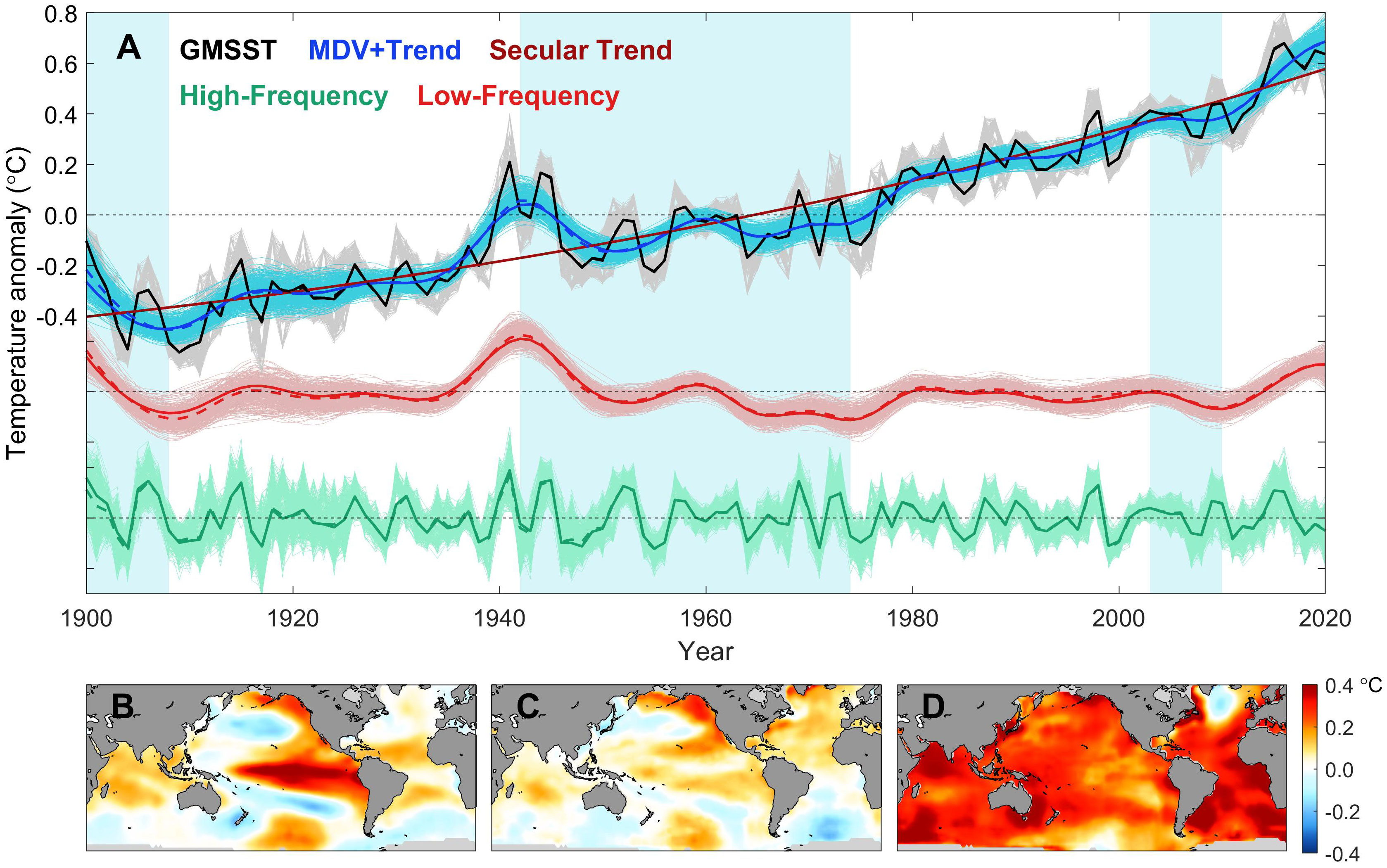
Figure 1 Multi-scale variability features of sea surface temperature. (A) EEMD decomposition of the GMSST (black solid line) based on annual-mean data. The high-frequency components (HFC, shorter than decadal), low-frequency components (LFC, longer than decadal), and secular trend (ST) are indicated with green, red, and brown solid lines, respectively. The dashed lines denote the ensemble mean of the light color lines. The blue lines, which are referred to as the multi-decadal variabilities (MDV), are the sum of the red and brown lines, regarded as a well-smoothed version of the original series. The uncertainty of the raw data, HFC, LFC, and MDV are estimated by the down-sampling method, shown in the light solid grey, green, red, and blue lines, respectively. The blue shading represents the periods of global warming slowdown. The climatology is based on the 1900-2020 mean. (B–D) Regression patterns of the GSST upon the HFC, LFC, and ST, respectively (Unit: °C). Note that these three components above are normalized firstly to unit standard deviation, and those grid points covered by ice during at least one-third of the period of 1900-2020 are filled with grey.
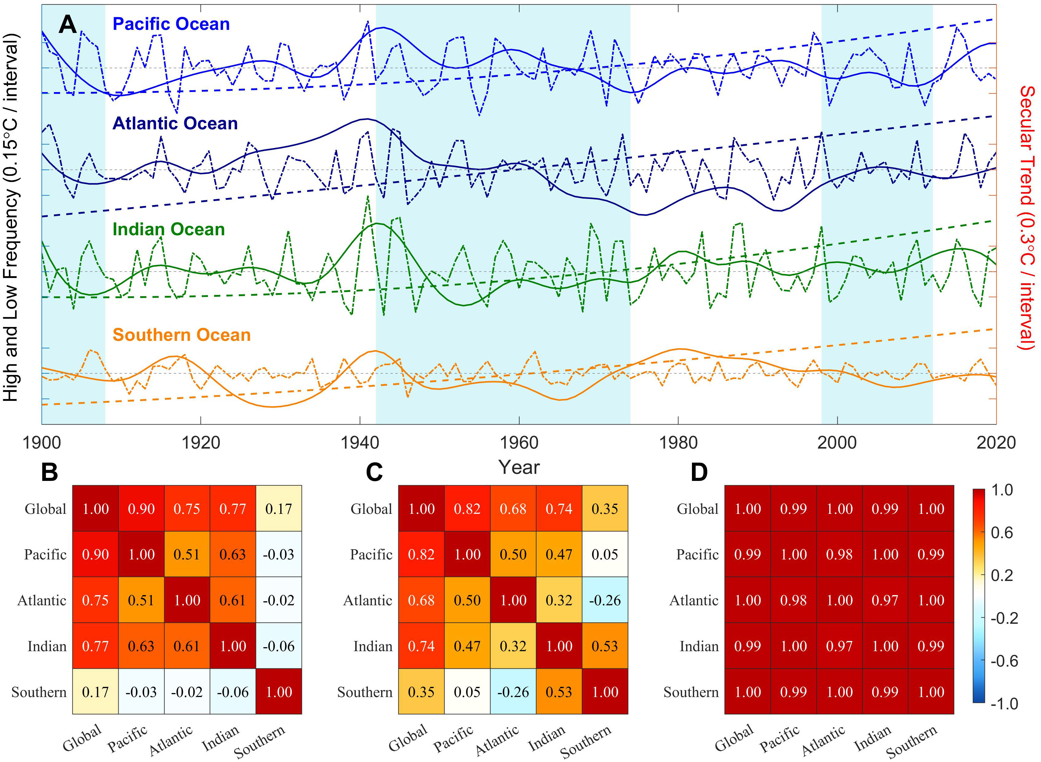
Figure 2 Multi-scale evolution features of the GMSST or regional-mean SST. (A) Evolution of the high-frequency components (dash-dotted lines), low-frequency components (solid lines), and secular trends (dashed lines) of the GMSST, the Pacific Ocean, the Atlantic Ocean, the Indian Ocean, and the Southern Ocean, respectively (unit: °C). Note that the values of secular trends should be referenced to the right axis. The blue shading represents global warming hiatus, same as Figure 1A. (B–D) The correlation coefficients of the high-frequency components, low-frequency components, and secular trends, among the GMSST, the Pacific Ocean, the Atlantic Ocean, the Indian Ocean, and the Southern Ocean, respectively. Note that the grids which do not pass the significance test (around 95% confidence level) have been colored white.
4 Variance contribution of multi-scale variabilities
Previous studies show that the evolution of the GMSST is typically dominated by the ST (e.g., Chen et al., 2017; Zhang et al., 2019; Xu et al., 2022). However, no more attention was paid to the local features. Here, benefiting from the spatial locality of the MEEMD method (Wu et al., 2009; Ji et al., 2014; Xu et al., 2021), the explained variance of the HFC, LFC, and ST will be analyzed grid-by-grid, respectively, based on the annual-mean SST data. The annual-mean data were used for the EEMD decomposition rather than monthly data since the explained variance of the extratropical regions’ annual cycle component might reach more than 90% (Stine, 2010; Vecchio et al., 2010), which would make it difficult to comprehend the other components.
Figure 3 exhibits the variance contributions (or explained variance) of these three components mentioned above at each grid point. The explained variance of the HFC in the equatorial central-east and south mid-latitude Pacific could reach more than 60%, and that in regions such as the North Pacific, the northern tropical Atlantic, the mid-latitude Atlantic in both hemispheres, and the Indo-western Pacific also exceed 40%. These grid points, which are primarily located in the subpolar North Atlantic and Southern Ocean in both the Pacific and Atlantic sectors, are those where the LFC variance contribution is greater than 40%. Meanwhile, the variance contribution of those grid points over the North Pacific and South Indian Ocean are also around 20-40%. The most significant discrepancies between the HFC and LFC patterns are centralized in the Pacific, with slight deviations in the tropical and subtropical Atlantic (see Figure S1). Turning to the ST, it is noted that the key characteristics are somewhat similar to those in Figure 1D, showing that the values greater than 60% are displayed in the tropical Indian Ocean in the northern hemisphere, the Southern Ocean, which extends from the tip of southwest Africa to the southern side of Australia, the Indo-western Pacific, east of the continents in both hemispheres, and the tropical Atlantic, whose areas are also the most noticeable regions where the ST differs markedly from the other two components (shown in Figure S1).
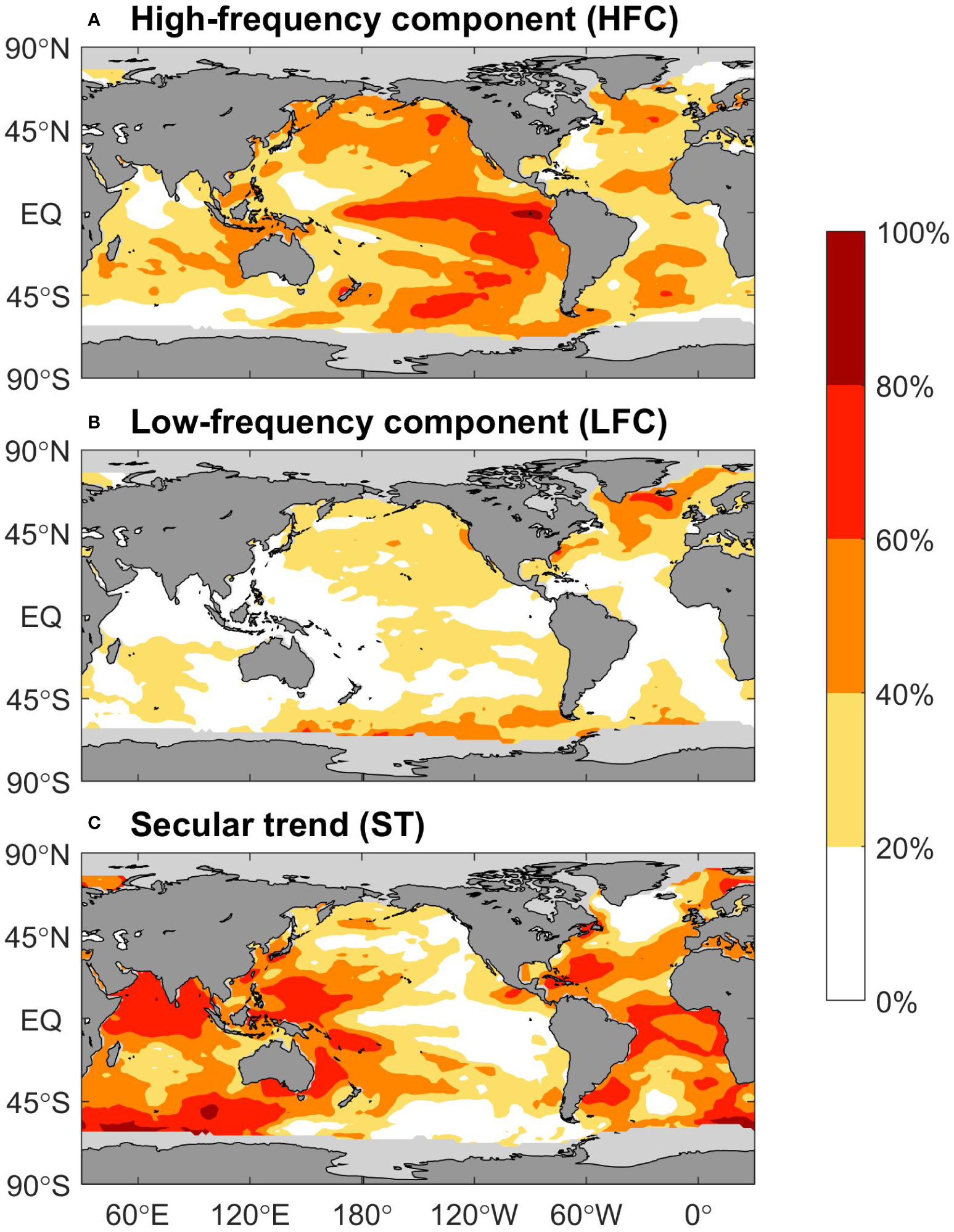
Figure 3 Variance contributions of (A) High-frequency component (HFC), (B) Low-frequency components, and (C), Secular trend at each grid (unit: %). Those grid points covered by ice during at least one-third of the period of 1900-2020 are all filled with grey. Note that for any specific grid point, the total variance contribution of these three parts above should be 100%.
The explained variances tied to different frequency bands among different ocean basins have remarkable discrepancies, so here we further investigate the multi-scale variability features of the mean SST in several regions, which is shown in Figures 4, 5. From a regional perspective, the secular trends of SST contribute to the largest part of the variance, suggesting that global warming still remains the most conspicuous feature (Figure 4A). It is also notable that the variance contributions of the HFC in the Pacific and the Indian Ocean are as many as two and three times higher than the GMSST, respectively (Figures 4A, B), which may be related to the interannual variabilities such as the ENSO and IOD. What’s more, it seems that the amplitude of the HFC in the Southern Ocean is smaller than that in the remaining three ocean basins, according to Figure 2A. Another feature is that the HFC of the Southern Ocean has little correlation with other regions (see Figure 2B), possibly as a result of its isolation, whereas the HFC of the Pacific, Atlantic, and Indian Oceans can interact or connect via some tropical physical processes (Li et al., 2016; Cai et al., 2019). In addition, the explained variances of the LFC in four basins are all approximately two times higher than that of the GMSST, with the largest one in the Atlantic (Figure 4A). The reason why the LFC of the GMSST has a smaller explained variance (Figure 4B) may be attributed to the superposition of positive and negative phases of the decadal to multi-decadal signals among different ocean basins.
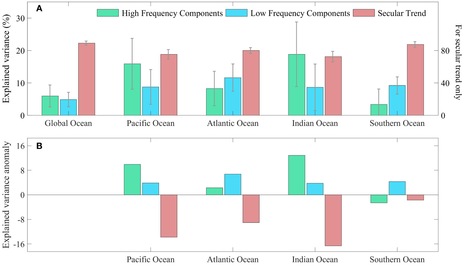
Figure 4 Variance contributions of multi-scale variabilities of the GMSST or regional averaged SST (unit: %). (A) Variance contributions and uncertainty interval (around 95% confidence level) of the high-frequency components, low-frequency components, and secular trends, for the GMSST, the Pacific Ocean, the Atlantic Ocean, the Indian Ocean, and the Southern Ocean, respectively. (B) Variance contribution anomaly of the four main ocean basins mentioned above relative to the GMSST. Note that all the error bars should be referenced to the left axis.
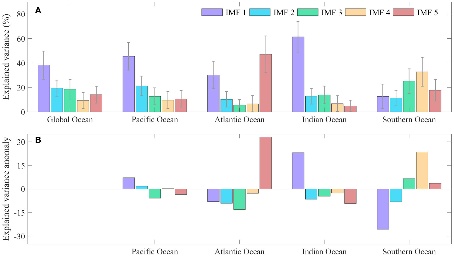
Figure 5 Variance contributions of the Intrinsic Mode Functions (IMFs) of the GMSST or regional averaged SST (unit: %). (A) Variance contributions and uncertainty interval (around 95% confidence level) of IMFs for the GMSST, the Pacific Ocean, the Atlantic Ocean, the Indian Ocean, and the Southern Ocean, respectively. (B) Variance contributions anomaly of the four main basins above relative to the GMSST. Note that the secular trends or residuals are not included here.
More specifically, Figure 5A presents the variance contribution of all the IMFs. Since the secular trend accounts for most of the explained variance for region-averaged SST, it is not involved in the discussion again here. As mentioned in the methods section, HFC is composed of IMF1 and IMF2. It shows that the HFC variance contribution in the Pacific and Indian Ocean, which are greater than GMSST, could be primarily traced back to the IMF1, with an estimated period of about 3-4 years (see Figure 5B and Table S1), roughly three times longer than the sampling frequency of the raw data. There is a well-recognized decadal oscillation signal, PDO, but the explained variances of IMF3 and IMF4 in the Pacific basin are not dramatically greater than the others (see Figure 5A). The reason may be that the explained variance of the LFC in the Pacific basin is highly diminished due to the offset of compensating patterns of PDO in the northwest and northeast Pacific (Chen and Tung, 2018a). However, the variance contribution of IMF5 is notably higher than the GMSST as well as the other ocean basins, which could be related to the AMO.
5 EOF analysis of the multi-scale variabilities
In this section, EOF analysis will be used to reveal the main spatio-temporal characteristics of monthly GSST in different frequency bands. Regarding monthly SST series, nine IMFs and a long-term trend can be obtained by the EEMD decomposition, according to Eq. (2). Based on the binary filter property of the EEMD method, the periods of IMF1 are approximately 3 months and IMF2 to IMF9 are twice as long as the former, respectively. In general, IMF1 represents the ultra-high frequency information of the intra-annual scale, while IMF2 and IMF3 contain annual cycle components, all of which are not involved in EOF analysis. Therefore, IMF3 to IMF6 are summed as the HFC, while IMF7 to IMF9 are summed as the LFC.
The three leading EOFs and PCs of the HFC of the monthly GSST are presented in Figure 6. The explained variance of the first mode (29.4%) is larger than the others. However, due to the orthogonality of the EOF approach, these spatial patterns have overlapping centers of action and perturbation polarities juxtaposed from visual observation, making it difficult to distinguish the signals at tropical and extratropical Pacific. To estimate the optimal angle for rotating EOF1-EOF3 patterns, an evaluation of the SASC metric proposed by Chen et al. (2017) is regarded as a critical reference. As mentioned in Section 2, the other two metrics named FASC and ‘trend transfer’ do not properly suit the discussion here, as the MEEMD decomposition has already separated the components of the GSST series at different time scales for each grid point. The rotation of the EOFs and PCs was performed in two steps. It is clarified that after each rotation step, the (R)EOFs and (R)PCs will be reordered according to the newest explained variance. Figures 7A, B) exhibit the values of the SASC as a function of the rotation angle, which are associated with the rotation between PC1 and PC3 (step (i)) as well as RPC2 and PC3 (step (ii)), respectively. All the curves in Figure 7 act as sinusoidal-like functions, but at different phase. The minimum evaluated values corresponding to step (i) and (ii) are at about 43° and 78°, with selected regions in (18°N-28°N, 172°W-152°W) and (10°S-10°N, 138°E-178°E), respectively. The modes after rotation are shown in Figure S2 (after the first step) and Figure 8. After pairwise rotation, it is found that the spatial patterns of REOF1 and REOF2 are predominantly concentrated in the central-eastern and central Pacific along the equator, respectively, representing ENSO diversity, i.e., EP and CP El Niño. The explained variances of these two rotated modes are very close (18.4% and 16.3%) and maintain orthogonality, indicating that besides being the dominant modes at interannual timescale, EP and CP El Niño also exhibit independent properties of each other, which aligns with the previous studies (e.g., Ashok et al., 2007; Ren and Jin, 2011; Timmermann et al., 2018).
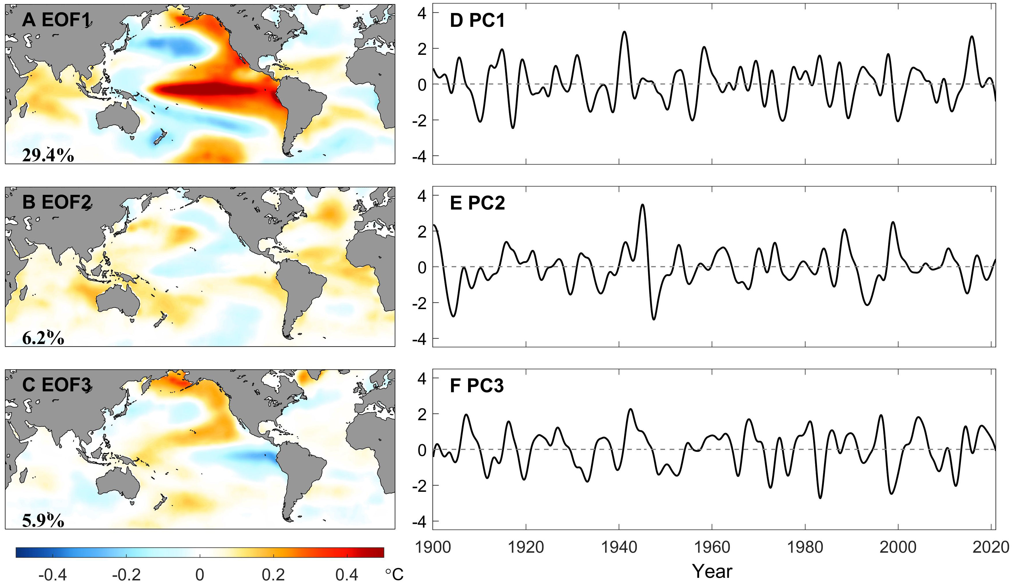
Figure 6 Conventional (i.e., unrotated) EOFs (left panel) and PCs (right panel) of the high-frequency components of monthly GSST extracted by the EEMD method for the period of record 1900-2020. Percentages of explained variance are printed at the bottom left on the EOF maps.
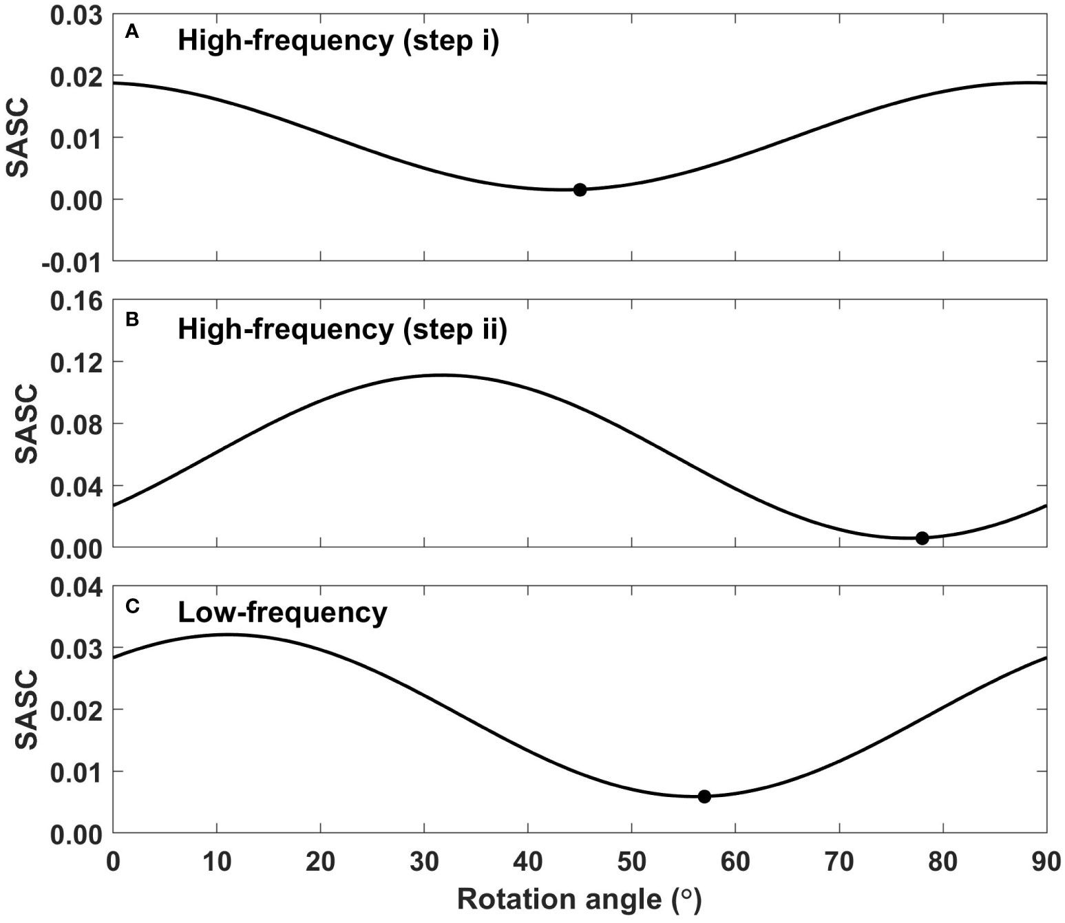
Figure 7 The spatially averaged squared covariance (SASC) metric is plotted as a function of the rotation angle. (A) pairwise rotation between PC1 and PC3 in Figure 6 (step i, EOFs and PCs are then re-ranked according to explained variance). (B) pairwise rotation between RPC2 and PC3 in Figure S1 (step ii). (C) pairwise rotation between PC1 and PC2 in Figure 9.
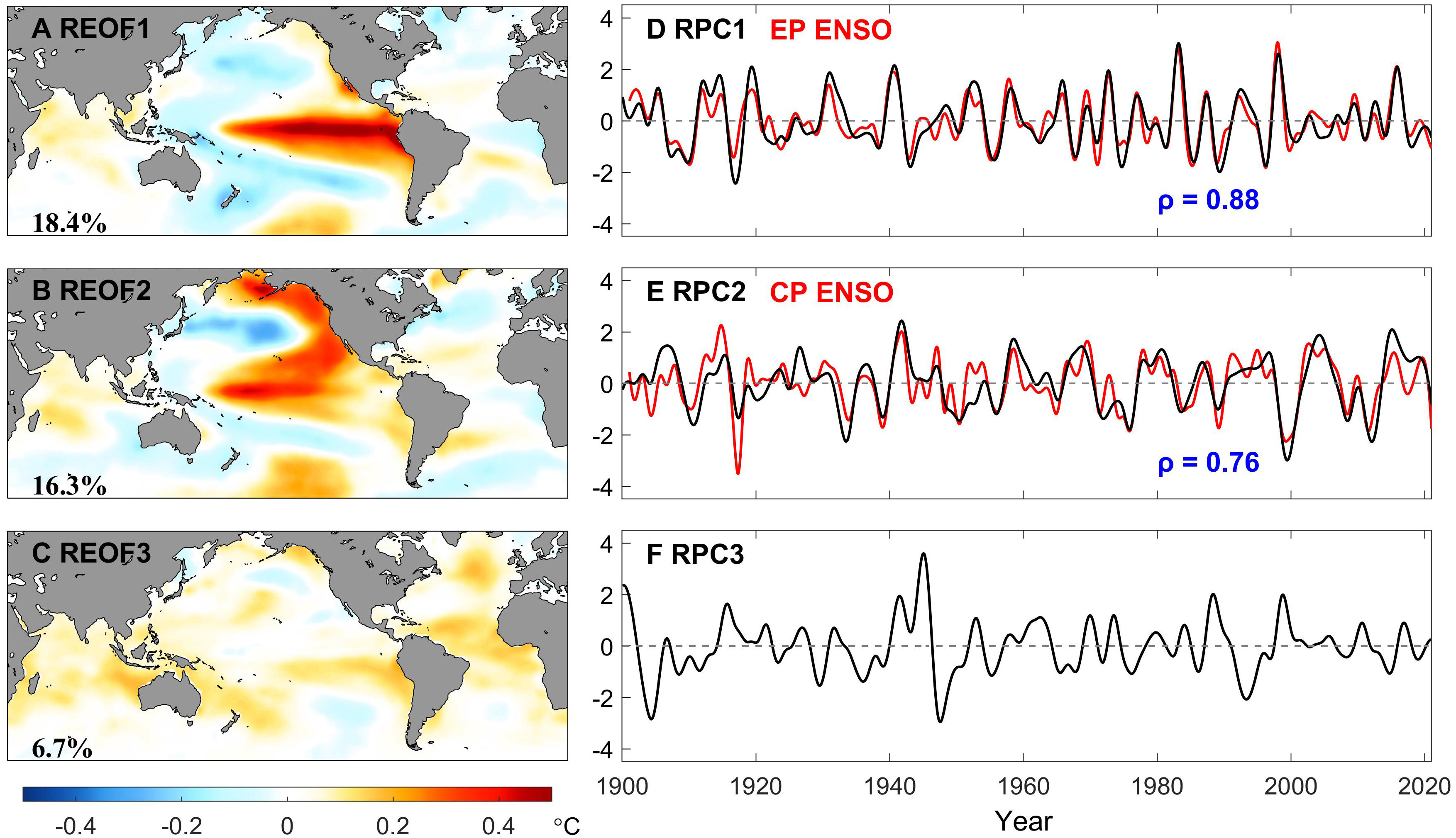
Figure 8 Pairwise-rotated EOFs (left panel) and PCs (right panel) of the high-frequency components of monthly GSST extracted by the EEMD method for the period of record 1900-2020 after both steps (i) and (ii). Percentages of explained variance are printed at the bottom left on the EOF maps. In the right panel, the high-frequency components of the EP El Niño and CP El Niño indices (sum of the IMFs 4-6) are shown by the red lines, while the blue values indicate their correlation coefficients with RPC1 and RPC2, respectively.
Parallelly, Figure 9 exhibits the two leading EOFs and PCs of the LFC, which explaines around 66% variance in total. It is reported that due to the orthogonality constraint of spatial modes, although EOF1 pattern has some AMO features, the signals in Pacific basin are also irrationally assigned, resulting in the mode mixing of the Atlantic and Pacific. Similarly, the SASC criterion is adopted to determine the optimal rotation angle under the target region (0°-66°N, 32°W-2°W), which is plotted in Figure 7C, for detaching the PDO and AMO. It is shown that the optimal rotation angle is 56°. The REOFs shown in Figure 10 are associated with the AMO-like and PDO-like patterns. However, as presented in REOF1, the positive AMO mode is accompanied by a cooling pattern of the equatorial Pacific, and vice versa. By analyzing the low-pass-filtered GSST data, Chen et al. (2017) argued that there exists an Atlantic-Pacific coupling, not an illusion caused by mode mixing, so that REOF cannot eliminate it through any angle in the two-dimensional phase space, but conversely, the PDO-like mode does not demonstrate an AMO-like pattern.
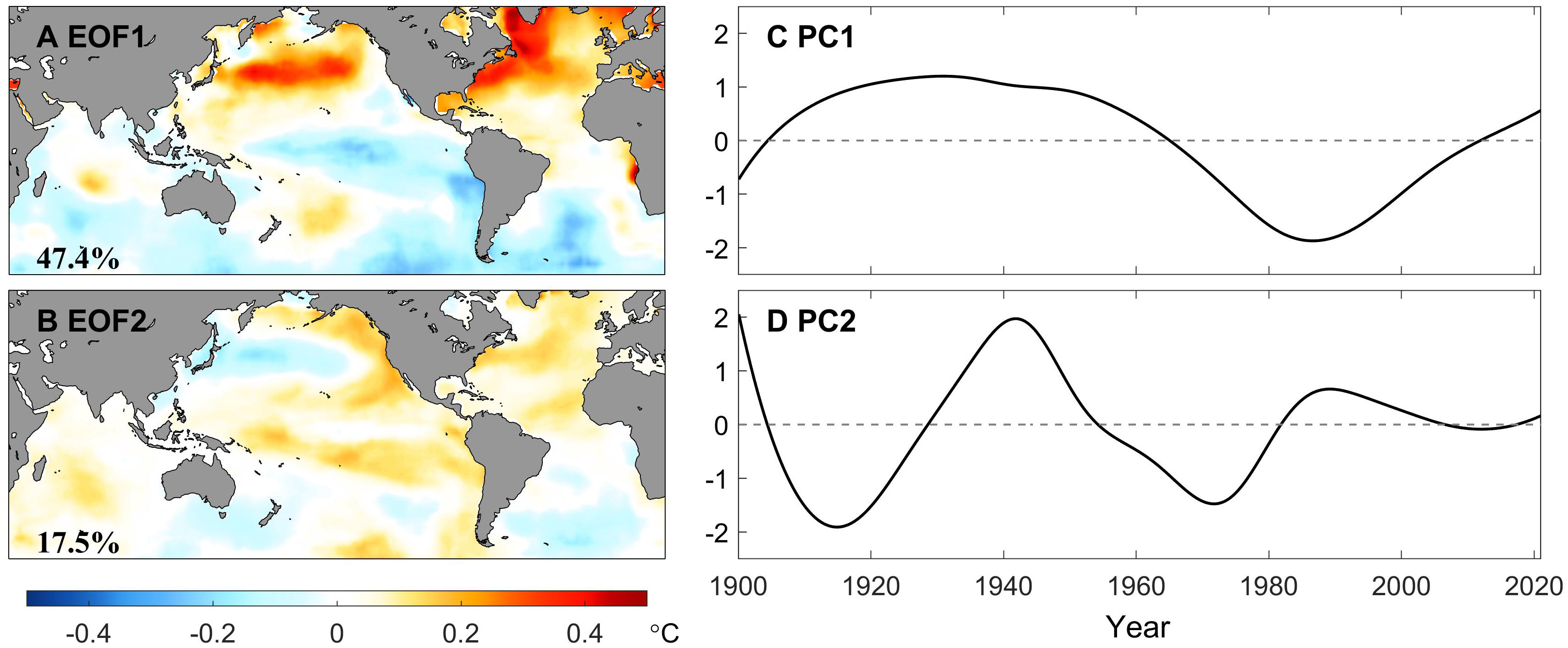
Figure 9 Conventional (i.e., unrotated) EOFs (left panel) and PCs (right panel) of the low-frequency components of monthly GSST extracted by the EEMD method for the period of record 1900-2020. Percentages of explained variance are printed at the bottom left on the EOF maps.
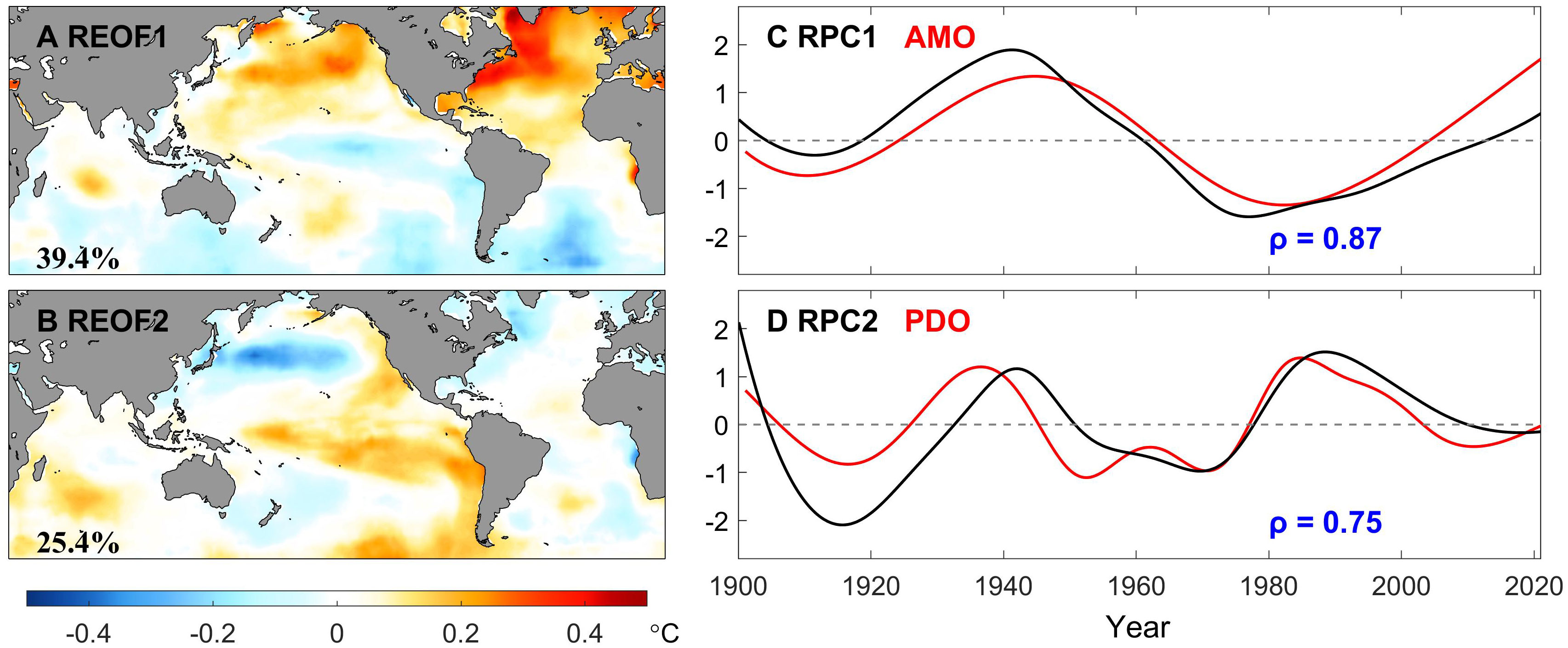
Figure 10 Pairwise-rotated EOFs (left panel) and PCs (right panel) of the low-frequency components of monthly GSST extracted by the EEMD method for the period of record 1900-2020. Percentages of explained variance are printed at the bottom left on the EOF maps. In the right panel, the low-frequency components of the AMO (total of IMFs 8-9) and PDO indices (total of IMFs 7-9) are shown by the red line, while the blue values indicate their correlation coefficients with RPC1 and RPC2, respectively.
Finally, the main features of the secular trend are displayed in Figure 11, which substantially matches the findings revealed by Xu et al. (2021, 2022) by portraying the EEMD trends. The two leading EOFs have explained almost all of the variance here, especially the EOF1 even reaching more than 95%. We argue that the EOF1 pattern, as well as the PC1, are mainly related to global warming, with almost everywhere showing the warming trend, except for the subpolar North Atlantic (cooling pattern), the tropical central Pacific, and the Southern Ocean in the Pacific sector (close to zero, implying no signal, according to Equation (3)). Unlike the monotonic increase of PC1, PC2 resembles a parabola with an upward opening. By combining the EOF2, the second mode depicts a secular trend of decrease followed by increasing in the equatorial central Pacific and the Southern Ocean in the Pacific sector (even very slightly), with the turning point around the middle of the last century. Just the opposite, several regions such as the North Pacific show a first upward followed by a downward trend. Although this feature is also represented in Figure 2 given by Xu et al. (2021), the discrepancies still exist and probably can be attributed to the fact that the secular trends are analyzed directly here, whereas they defined the EEMD trend first.
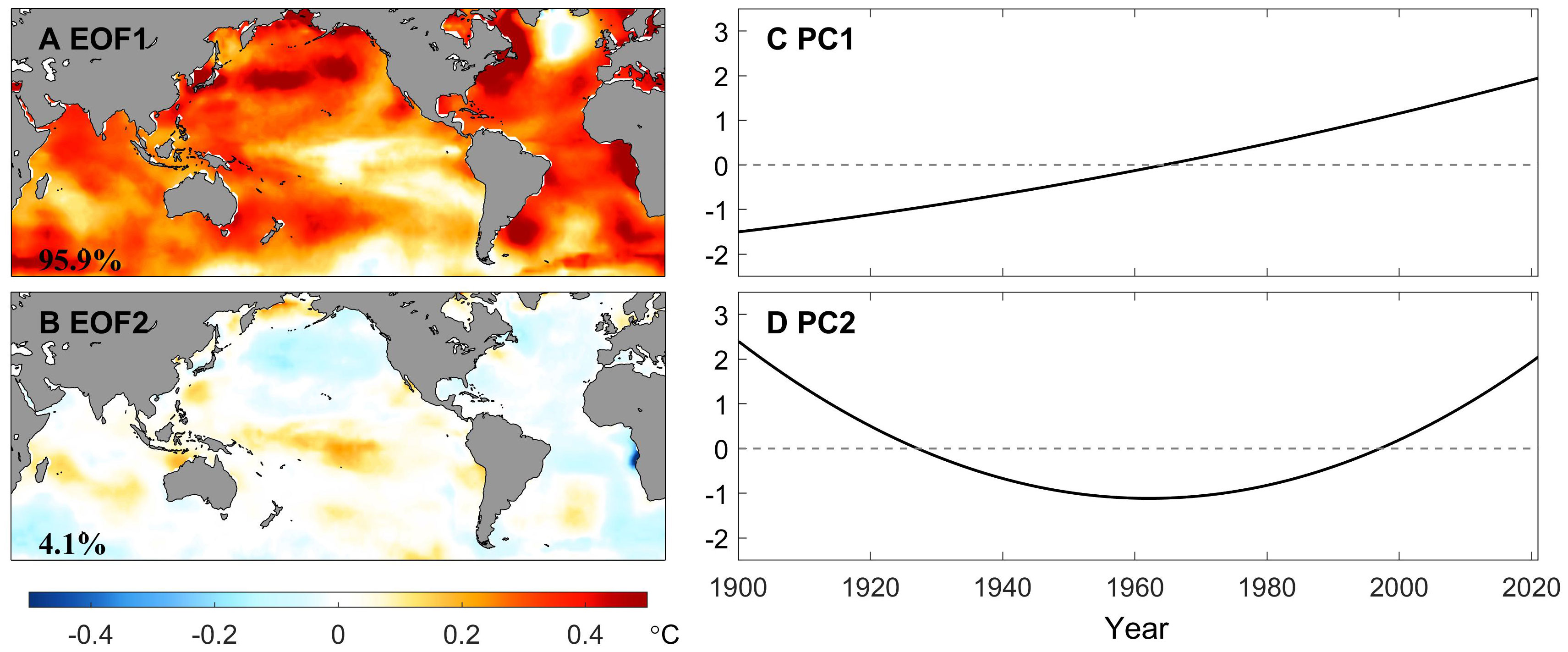
Figure 11 Conventional (i.e., unrotated) EOFs (left panel) and PCs (right panel) of the secular trends of monthly GSST extracted by the EEMD method for the period of record 1900-2020. Percentages of explained variance are printed at the bottom left on the EOF maps.
6 Conclusions and discussions
In this study, the EEMD method is applied grid-by-grid to extract the multi-scale variabilities of the GSST. By superimposing the IMFs in nearly frequency bands, the HFC, LFC, and ST at each grid point are obtained, respectively. It is found that the global warming slowdown is highly modulated by the LFC signals stuck in a downward stage, as the decadal to multi-decadal oscillations in the four main ocean basins are mostly in the downward or negative phases. By regressing the GSST onto the HFC, LFC, and ST, we also found that the pattern of the HFC is associated with the ENSO, NTAM, SSAM, and IOBM at low latitudes, as well as the PDO-like and SPDO-like patterns at mid-latitudes, which are induced by tropical Pacific variabilities through the atmospheric bridge. The LFC shows a horseshoe-shaped pattern in North Pacific and an interhemispheric dipole in the Atlantic, related to the PDO and AMO, respectively. With the exception of the subpolar North Atlantic, the ST’s regressing pattern is almost always positive. Larger values are primarily found in the tropical Indian Ocean in the northern hemisphere, the Southern Ocean surrounding southern Africa, the southeast coast of Australia, east of the continents in both hemispheres connected to the western boundary currents with their mid-latitude extensions, and the eastern tropical Atlantic.
By taking advantage of the spatial locality of the MEEMD method, the variance contributions of multi-scale variabilities for each grid point are explored. It has been also revealed that the explained variance of the HFC in the equatorial central-eastern Pacific, and the mid-latitude Pacific in the southern hemisphere could reach more than 60%, whereas the pattern of the LFC is mainly concentrated in subpolar North Atlantic and the Southern Ocean in both Pacific and Atlantic sectors, larger than 40%. The explained variance of the ST hitting beyond 60% is widely throughout the Indian Ocean in the northern hemisphere, the Southern Ocean from the tip of southwest Africa expanded to the southern side of Australia, the Indo-western Pacific, east of the continents in both hemispheres, and the tropical Atlantic. Moreover, the relative variance contributions of the multi-scale variabilities of specific IMFs are further analyzed in several ocean basins, exhibiting characteristics from a regional mean perspective.
The main space-time modes of the variabilities in different frequency bands obtained by EOF analysis show unjustified mixing. Therefore, pairwise rotation is then applied for eliminating the overlapping centers with opposite polarities, which is regarded as a compensator for the regions with the same polarity, enabling the orthogonality of the spatial modes. It is identified that on the high frequency band, ENSO diversity is the dominant, characterized by the presence of CP and EP El Niño in the first two REOF modes, while regarding the low frequency band, the AMO and PDO emerge. It can thus be concluded that the diversity of ENSO, manifesting as EP and CP El Niño, constitutes two primary orthogonal axes on the interannual scale. Meanwhile, when considering the decadal to multi-decadal scales, the AMO and PDO stand out as the key axes, which could be viewed as an extension to the findings of Chen et al. (2017).
There are still some shortages that need to discuss. On the one hand, it has to be admitted that in the early record period as well as during World War II, the scarcity of raw data and the backwardness of observation tools resulted in the poor quality of reconstructed SST data jointly, which perhaps caused a large uncertainty. On the other hand, for those signals with periods longer than decadal, it is so hard to meet statistically significant when we calculate their correlation coefficients with the RPCs due to an extremely few statistical degrees of freedom caused by limited historical record length. Despite these, we still insist that the results gained from the pairwise rotated EOF analysis are enlightening. Besides, deeper mechanisms of these features still need to be further explored, and we also face more blank about how these nonlinear modulated among these ocean basins.
All in all, the purpose of this work is trying to find a novel solution or perspective for the analysis of the multi-scale variabilities, which we are strongly convinced is beneficial to have a better comprehension of the global climate change for both the past and future, even in the slightest hint. It is also worth noting that the multi-scale variability of GSST holds significant implications for atmospheric variables. For instance, overall, under global warming, the long-term increasing trend of the SST may contribute to the intensification of tropical cyclones (TCs), which has been substantiated through observations (e.g., Sobel et al., 2016; Wang et al., 2022), theoretical analyses (Emanuel, 1987), and numerical experiments (Knutson and Tuleya, 2004; Knutson et al., 2020; Emanuel, 2021). However, on a regional scale, internal variability, such as the Interdecadal Pacific Oscillation (IPO), can also exert a significant regulatory impact on TCs’ activity (Zhao et al., 2020). Consequently, how the multi-scale variabilities of GSST influence atmospheric variables and its future evolution, still deserves further research.
Data availability statement
Publicly available datasets were analyzed in this study. This data can be found here: NOAA_ERSST_V5 data provided by the NOAA/OAR/ESRL PSD, Boulder, Colorado, USA, from their website at https://www.esrl.noaa.gov/psd/.
Author contributions
ZX, GH, and FJ conceived this study. ZX led to writing the initial manuscript in discussion with FJ. ZX did the data analysis and produced figures. FJ improved this manuscript. All authors contributed to the article and approved the submitted version.
Funding
This work was jointly supported by the National Natural Science Foundation of China (42141019, 41831175, 91937302, 41721004, 42275034 and 42075029), and Strategic Priority Research Program of Chinese Academy of Sciences (XDA20060501). The first author, ZX, was supported by China Scholarship Council (CSC) during his exchanged study at the University of Tokyo.
Acknowledgments
We thank Prof. Xiaoyao Chen for providing data analysis codes and useful discussions. Mr. Jinshuo Wang and Mr. Chenglin Lv provided several technical supports in MATLAB. We would also like to thank Mr. Hongzhao Sun for helpful mathematical analysis suggestions. NOAA_ERSST_V5 data is provided by the NOAA/OAR/ESRL PSD, Boulder, Colorado, USA, from their website at https://www.esrl.noaa.gov/psd/. The other climate indices are all available at https://icar.nuist.edu.cn/main.htm, https://ds.data.jma.go.jp/tcc/tcc/products/elnino/decadal/pdo.html, and http://www.psl.noaa.gov/data/timeseries/AMO.
Conflict of interest
The authors declare that the research was conducted in the absence of any commercial or financial relationships that could be construed as a potential conflict of interest.
Publisher’s note
All claims expressed in this article are solely those of the authors and do not necessarily represent those of their affiliated organizations, or those of the publisher, the editors and the reviewers. Any product that may be evaluated in this article, or claim that may be made by its manufacturer, is not guaranteed or endorsed by the publisher.
Supplementary material
The Supplementary Material for this article can be found online at: https://www.frontiersin.org/articles/10.3389/fmars.2023.1238320/full#supplementary-material
References
Ashok K., Behera S. K., Rao S. A., Weng H., Yamagata T. (2007). Modoki and its possible teleconnection. J. Geophys. Res. Oceans 112 (C11). doi: 10.1029/2006JC003798
Ashok K., Yamagata T. (2009). Climate change: The El Niño with a difference. Nature 461 (7623), 481–484. doi: 10.1038/461481a
Bjerknes J. (1972). Large-scale atmospheric response to the 1964–65 Pacific equatorial warming. J. Phys. Oceanogr. 2, 212–217. doi: 10.1175/1520-0485(1972)002<0212:LSARTT>2.0.CO;2
Brown P. T., Li W., Cordero E. C., Mauget S. A. (2015). Comparing the model-simulated global warming signal to observations using empirical estimates of unforced noise. Sci. Rep. 5 (1), 1–9. doi: 10.1038/srep09957
Cai W., Wu L., Lengaigne M., Li T., McGregor S., Kug J. S., et al. (2019). Pantropical climate interactions. Science 363, eaav4236. doi: 10.1126/science.aav4236
Chen X. Y., Feng Y., Huang N. E. (2014). Global sea level trend during 1993–2012 Global Planet. Change 112 (2014), 26–32. doi: 10.1016/j.gloplacha.2013.11.001
Chen X., Tung K. K. (2018a). Global-mean surface temperature variability: space-time perspective from rotated EOFs. Clim. Dyn. 51, 1719–1732. doi: 10.1007/s00382-017-3979-0
Chen X. Y., Tung K.-K. (2018b). Global surface warming enhanced by weak Atlantic overturning circulation. Nature 559, 387–391. doi: 10.1038/s41586-018-0320
Chen X. Y., Wallace J. M. (2015). ENSO-like variability: 1900-2013. J. Climate 28 (24), 9623–9641. doi: 10.1175/JCLI-D-15-0322.1
Chen X. Y., Wallace J. M. (2016). Orthogonal PDO and ENSO indices. J. Climate 29, 3883–3892. doi: 10.1175/JCLI-D-15-0684.1
Chen X. Y., Wallace J. M., Tung K.-K. (2017). Pairwise-rotated EOFs of global SST. J. Climate 30, 5473–5489. doi: 10.1175/JCLI-D-16-0786.1
Chen X., Zhang Y., Zhang M., Feng Y., Wu Z., Qiao F., et al. (2013). Intercomparison between observed and simulated variability in global ocean heat content using empirical mode decomposition, part I: modulated annual cycle. Clim. Dyn. 41 (11-12), 2797–2815. doi: 10.1007/s00382-012-1554-2
Coleman C. D. (2022). Improved complete ensemble empirical mode decompositions with adaptive noise of global, hemispherical and tropical temperature anoMalies 1850–2021. Theor. Appl. Climatol 150, 35–52. doi: 10.1007/s00704-022-04064-x
Delworth T. L., Mann M. E. (2000). Observed and simulated multidecadal variability in the Northern Hemisphere. Clim. Dyn. 16, 661–676. doi: 10.1007/s003820000075
Deser C., Alexander M. A., Xie S.-P., Phillips A. S. (2010). Sea surface temperature variability: patterns and mechanisms. Annu. Rev. Mar. Sci. 2, 115–143. doi: 10.1146/annurev-marine-120408-151453
Dommenget D., Bayr T., Frauen C. (2013). Analysis of the non-linearity in the pattern and time evolution of El Niño southern oscillation. Clim. Dyn. 40, 2825–2847. doi: 10.1007/s00382-012-1475-0
Dommenget D., Latif M. (2008). Generation of hyper climate modes. Geophys. Res. Lett. 35, L02706. doi: 10.1029/2007GL031087
Drijfhout S., van Oldenborgh G. J., Cimatoribus A. (2012). Is a Decline of AMOC causing the warming hole above the North Atlantic in observed and modeled warming patterns? J. Clim. 25 (24), 8373–8379. doi: 10.1175/JCLI-D-12-00490.1
Emanuel K. A. (1987). The dependence of hurricane intensity on climate. Nature 326, 483–485. doi: 10.1038/326483a0
Emanuel K. (2021). Response of global tropical cyclone activity to increasing CO2: results from downscaling CMIP6 models. J. Clim. 34, 57–70. doi: 10.1175/JCLI-D-20-0367.1
Enfield D. B., Mestas-Nunez A. M., Trimble P. J. (2001). The Atlantic multidecadal oscillation and its relation to rainfall and river flows in the continental U.S. Geophys. Res. Lett. 28, 2077–2080. doi: 10.1029/2000GL012745
Feng Y., Chen X., Tung K. K. (2020a). ENSO diversity and the recent appearance of Central Pacific ENSO. Clim. Dyn. 54, 413–433. doi: 10.1007/s00382-019-05005-7
Feng Y., Tung K. K. (2020b). ENSO modulation: real and apparent; implications for decadal prediction. Clim. Dyn. 54, 615–629. doi: 10.1007/s00382-019-05016-4
Flandrin P., Goncalves P. (2004). Empirical mode decompositions as data-driven wavelet-like expansions. Int. J. Wavelets Multiresolut. Inf. Process. 2, 477–496. doi: 10.1142/S0219691304000561
Folland C. K., Palmer T. N., Parker D. E. (1986). Sahel rainfall worldwide sea temperatures. Nature 320 (6063), 602–606. doi: 10.1038/320602a0
Franzke C. (2009). Multi-scale analysis of teleconnection indices: climate noise and nonlinear trend analysis. Nonlinear Processes Geophysics 16, 65–76. doi: 10.5194/npg-16-65-2009
Freeman E., Woodruff S. D., Worley S. J., Lubker S. J., Kent E. C., Angel W. E., et al. (2017). ICOADS Release 3.0: A major update to the historical marine climate record. Int. J. Climatol. 37, 2211–2232. doi: 10.1002/joc.4775
Huang B., Angel W., Boyer T., Cheng L., Chepurin G., Freeman E., et al. (2018). Evaluating SST analyses with independent ocean profile observations. J. Climate 31, 5015–5030. doi: 10.1175/JCLI-D-17-0824.1
Huang B., Banzon V. F., Freeman E., Lawrimore J., Liu W., Peterson T. C., et al. (2014). Extended Reconstructed Sea Surface Temperature version 4 (ERSST.v4): Part I. Upgrades and intercomparisons. J. Climate 28, 911–930. doi: 10.1175/JCLI-D-14-00006.1
Huang B., Thorne P. W., Banzon V. F., Boyer T., Chepurin G., Lawrimore J. H., et al. (2017a). Extended Reconstructed Sea Surface Temperature version 5 (ERSSTv5), Upgrades, validations, and intercomparisons. J. Climate 30 (20), 8179–8205. doi: 10.1175/JCLI-D-16-0836.1
Huang N. E., Shen Z., Long S. R., Wu M. C., Shih H. H., Zheng Q., et al. (1998). The empirical mode decomposition and the Hilbert spectrum for nonlinear and non-stationary time series analysis. Proc. R Soc. Lond. A Math Phys. Sci. 454, 903–995. doi: 10.1098/rspa.1998.0193
Huang B., Shukla J. (2005). Ocean-atmosphere interactions in the tropical and subtropical Atlantic ocean. J. Climate 18 (11), 1652–1672. doi: 10.1175/JCLI3368.1
Huang B., Thorne P. W., Smith T. M., Liu W., Lawrimore J., Banzon V. F., et al (2016). Further exploring and quantifying uncertainties for extended reconstructed sea surface temperature (ERSST) version 4 (v4). J. Climate 29, 3119–3142. doi: 10.1175/JCLI-D-15-0430.1
Huang N. E., Wu Z. (2008). A review on Hilbert-Huang transform: Method and its applications to geophysical studies. Rev. Geophys. 46 (2). doi: 10.1029/2007RG000228
Huang J., Xie Y., Guan X., Li D., Ji F. (2017b). The dynamics of the warming hiatus over the Northern Hemisphere. Clim. Dyn. 48, 424–446. doi: 10.1007/s00382-016-3085-8
Huang G., Xu Z., Qu X., Cao J., Long S., Yang K., et al. (2022). Critical climate issues towards carbon neutrality targets. Fundam. Res. 2 (3), 396–400. doi: 10.1016/j.fmre.2022.02.011
IPCC. (2013). “Climate change 2021: the physical science basis,” in Contribution of working group I to the fifth assessment report of IPCC the intergovernmental panel on climate change Eds Stocker T. F., Qin D., Plattner G. K., Tignor M. M., Allen S. K., Boschung. J. (Cambridge University Press), 1535.
IPCC. (2021). “Climate change 2021: the physical science basis,” in Contribution of working group I to the sixth assessment report of the intergovernmental panel on climate change. Eds. Masson-Delmotte V., Zhai P., Pirani A., Connors S. L., Péan C., Berger S. B, et al. (IPCC), 2.
Ji F., Wu Z., Huang J., Chassignet E. P. (2014). Evolution of land surface air temperature trend. Nat. Clim. Chang. 4, 462–466. doi: 10.1038/nclimate2223
Kaiser H. F. (1958). The varimax criterion for analytic rotation in factor analysis. Psychometrika 23, 187–200. doi: 10.1007/BF02289233
Knight J. R., Allan R. J., Folland C. K., Vellinga M. (2005). A signature of persistent natural thermohaline circulation cycles in observed climate. Geophys Res. Lett. 32 (20). doi: 10.1029/2005GL024233
Knutson T., Camargo S. J., Chan J. C., Emanuel K., Ho C. H., Kossin J., et al. (2020). Tropical cyclones and climate change assessment: Part II: projected response to anthropogenic warming. Bull. Amer. Meteor. Soc. 101, E303–E322. doi: 10.1175/BAMS-D-18-0194.1
Knutson T. R., Tuleya R. E. (2004). Impact of CO2-induced warming on simulated hurricane intensity and precipitation: Sensitivity to the choice of climate model and convective parameterization. J. Clim. 17, 3477–3495. doi: 10.1175/1520-0442(2004)017<3477:IOCWOS>2.0.CO;2
Kosaka Y., Xie S.-P. (2013). Recent global-warming hiatus tied to equatorial Pacific surface cooling. Nature 501, 403–407. doi: 10.1038/nature12534
Kosaka Y., Xie S.-P. (2016). The tropical pacific as a key pacemaker of the variable rates of global warming. Nat. Geosci 9, 669–673. doi: 10.1038/ngeo2770
Kug J. S., Jin F. F., An S. I. (2009). Two types of el Niño events: Cold tongue El Niño and warm pool El Niño. J. Clim. 22 (6), 1499–1515. doi: 10.1175/2008JCLI2624.1
Lau K. M., Wu H. T., Bony S. (1997). The role of large-scale atmospheric circulation in the relationship between tropical convection and sea surface temperature. J. Clim 10 (3), 381–392. doi: 10.1175/1520-0442(1997)010<0381:TROLSA>2.0.CO;2
Li Y., Ge J., Dong Z., Hu X., Yang X., Wang M., et al. (2021). Pairwise-rotated EOFs of global cloud cover and their linkages to sea surface temperature. IntJ Climatol. 41, 2342–2359. doi: 10.1002/joc.6962
Li X., Xie S. P., Gille S. T., Yoo C.. (2016). Atlantic-induced pan-tropical climate change over the past three decades. Nat. Clim. Change. 6, 275–279. doi: 10.1038/nclimate2840
Liu W., Huang B., Thorne P. W., Banzon V. F., Zhang H. M., Freeman E., et al. (2015). Extended Reconstructed Sea Surface Temperature version 4 (ERSST.v4): Part II. Parametric and structural uncertainty estimations. J. Climate 28, 931–951. doi: 10.1175/JCLI-D-14-00007.1
Mann M. E., Park J. (1994). Global-scale modes of surface temperature variability on interannual to century timescales. J. Geophys. Res. 99, 25819. doi: 10.1029/94JD02396
Mann M. E., Steinman B. A., Brouillette D. J., Miller S. K.. (2021). Multidecadal climate oscillations during the past millennium driven by volcanic forcing. Science 371 (6533), 1014–1019. doi: 10.1126/science.abc5810
Mann M. E., Steinman B. A., Miller S. K. (2020). Absence of internal multidecadal and interdecadal oscillations in climate model simulations. Nat. Commun. 11, 49. doi: 10.1038/s41467-019-13823-w
Mantua N. J., Hare S. R., Zhang Y., Wallace J. M., Francis R. C. (1997). A Pacific interdecadal climate oscillation with impacts on salmon production. Bull. Am. Meteorol. Soc. 78 (6), 1069–1079. doi: 10.1175/1520-0477(1997)078<1069:APICOW>2.0.CO;2
Marshall J., Scott J. R., Armour K. C., Campin J. M., Kelley M., Romanou A. (2015). The oceans role in the transient response of climate to abrupt greenhouse gas forcing. Clim Dyn. 44, 2287–2299. doi: 10.1007/s00382-014-2308-0
McPhaden M. J., Zebiac S. E., Glantz M. H. (2006). ENSO as an integrating concept in earth science. Science 314, 1740–1745. doi: 10.1126/science.1132588
Minobe S. (1999). Resonance in bidecadal and pentadecadal climate oscillations over the North Pacific: role in climatic regime shifts. Geophys Res. Lett. 26 (7), 855–858. doi: 10.1029/1999GL900119
Newman M., Alexander M. A., Ault T. R., Cobb K. M., Deser C., Di Lorenzo E., et al. (2016). The pacific decadal oscillation, revisited. J. Clim. 29 (12), 4399–4427. doi: 10.1175/JCLI-D-15-0508.1
Niu M., Gan K., Sun S., Li F. (2017). Application of decomposition-ensemble learning paradigm with phase space reconstruction for day-ahead PM2.5 concentration forecasting. J. Environ. Manage. 196, 110–118. doi: 10.1016/j.jenvman.2017.02.071
North G. R., Bell T. L., Cahalan R. F., Moeng F. J. (1982). Sampling errors in the estimation of empirical orthogonal functions. Mon. Wea. Rev. 110, 699–706. doi: 10.1175/1520-0493(1982)110<0699:SEITEO>2.0.CO;2
Qian C., Wu Z., Fu C., Zhou T. (2010). On multi-timescale variability of temperature in China in modulated annual cycle reference frame. Adv. Atmospheric Sci. 27, 1169–1182. doi: 10.1007/s00376-009-9121-4
Quadrelli R., Bretherton C. S., Wallace J. M. (2005). On sampling errors in empirical orthogonal functions. J. Climate 18, 3704–3710. doi: 10.1175/JCLI3500.1
Rasmusson E. M., Carpenter T. H. (1982). Variations in the tropical sea surface temperature and surface wind fields associated with the Southern Oscillation–El Niño. Mon. Wea. Rev. 110, 354–384. doi: 10.1175/1520-0493(1982)110<0354:VITSST>2.0.CO;2
Rayner N. A., Parker D. E., Horton E., Folland C. K., Alexander L. V., Rowell D. P., et al. (2003). Global analyses of sea surface temperature, sea ice, and night marine air temperature since the late nineteenth century. J. Geophys. Res. 108, 4407. doi: 10.1029/2002JD002670
Ren H. L., Jin F. F. (2011). Niño indices for two types of ENSO. Geophys. Res. Lett. 38 (4). doi: 10.1029/2010GL046031
Richman M. B. (1986). Rotation of principal components. J. Climatol. 6, 293–335. doi: 10.1002/joc.3370060305
Saji N. H., Goswami B. N., Vinayachandran P. N., Yamagata T.. (1999). A dipole mode in the tropical Indian Ocean. Nature 401, 360–363. doi: 10.1038/43854
Sarachik E., Cane M. A. (2010). The El Nino-Southern oscillation phenomenon (Cambridge: Cambridge University Press).
Schlesinger M. E., Ramankutty N. (1994). An oscillation in the global climate system of period 65–70 years. Nature 367, 723–726. doi: 10.1038/367723a0
Schlesinger B. M., Ramankutty N., Andronova N. (2000). Temperature oscillations in the north atlantic. Science 28, 547–548. doi: 10.1126/science.289.5479.547b
Sobel A. H., Camargo S. J., Hall T. M., Lee C. Y., Tippett M. K., Wing A. A.. (2016). Human influence on tropical cyclone intensity. Science 353, 242–246. doi: 10.1126/science.aaf6574
Sullivan A., Luo J.-J., Hirst A. C., Bi D., Cai W., He J. (2016). Robust contribution of decadal anoMalies to the frequency of central-Pacific El Niño. Sci. Rep. 6, 38540. doi: 10.1038/srep38540
Takahashi K., Montecinos A., Goubanova K., Dewitte B. (2011). ENSO regimes: Reinterpreting the canonical and Modoki El Niño. Geophys. Res. Lett. 38, L10704. doi: 10.1029/2011GL047364
Timmermann A., An S. I., Kug J. S., Jin F. F., Cai W., Capotondi A., et al. (2018). El niño–southern oscillation complexity. Nature 559, 535–545. doi: 10.1038/s41586-018-0252-6
Trenberth, Hoar T. J. (1997). El Niño and climate change. Geophys. Res. Lett. 24, 3057–3060. doi: 10.1029/97GL03092
Trenberth K. E., Shea D. J. (2006). Atlantic hurricanes and natural variability in 2005. Geophys. Res. Lett. 33, L12704. doi: 10.1029/2006GL026894
Trenberth K. E., Stepaniak D. P. (2001). Indices of el Niño evolution. J. Clim. 14, 1697–1701. doi: 10.1175/1520-0442(2001)014<1697:LIOENO>2.0.CO;2
Vecchio A., Capparelli V., Carbone V. (2010). The complex dynamics of the seasonal component of USA’s surface temperature. Atmospheric Chem. Phys. 10 (19), 9657–9665. doi: 10.5194/acp-10-9657-2010
Wang G., Wu L., Mei W., Xie S. P. (2022). Ocean currents show global intensification of weak tropical cyclones. Nature 611, 496–500. doi: 10.1038/s41586-022-05326-4
Webster P. J., Moore A. M., Loschnigg J. P., Leben R. R. (1999). Coupled ocean–atmosphere dynamics in the Indian Ocean during 1997–1998. Nature 401, 356–360. doi: 10.1038/43848
Wei M., Qiao F., Guo Y., Deng J., Song Z., Shu Q., et al. (2019). Quantifying the importance of interannual, interdecadal and multidecadal climate natural variabilities in the modulation of global warming rates. Clim. Dyn. 53, 6715–6672. doi: 10.1007/s00382-019-04955-2
Wilks D. S. (2011). Statistical Methods in the Atmospheric Sciences. 3rd Edition, (Academic Press: Oxford).
Woollings T., Gregory J. M., Pinto J. G., Reyers M., Brayshaw D. J. (2012). Response of the North Atlantic storm track to climate change shaped by ocean-atmosphere coupling. Nat. Geosci. 5, 313–317. doi: 10.1038/ngeo1438
Wu Z., Huang N. E. (2004). A study of the characteristics of white noise using the empirical mode decomposition method. Proc. R. Soc Lond. A. 460, 1597–1611. doi: 10.1098/rspa.2003.1221
Wu Z., Huang N. E. (2009). Ensemble empirical mode decomposition: A noise-assisted data analysis method. Adv. Adapt Data Anal. 01, 1–41. doi: 10.1142/S1793536909000047
Wu Z., Huang N. E. (2010). On the filtering properties of the empirical mode decomposition. Adv. Adapt. Data Anal. 2, 397–414. doi: 10.1142/S1793536910000604
Wu Z., Huang N. E., Chen X. (2009). The multi-dimensional ensemble empirical mode decomposition method. Adv. Adapt Data Anal. 01, 339–372. doi: 10.1142/S1793536909000187
Wu Z., Huang N. E., Long S. R., Peng C. K. (2007). On the trend, detrending, and variability of nonlinear and nonstationary time series. Proc. Natl. Acad. Sci. U.S.A. 104, 14889–14894. doi: 10.1073/pnas.0701020104
Wu Z., Huang N. E., Wallace J. M., Smoliak B. V., Chen X.. (2011). On the time-varying trend in global-mean surface temperature. Clim. Dyn. 37 (3–4), 759–773. doi: 10.1007/s00382-011-1128-8
Wu W., Ji F., Hu S., He Y., Wei Y., Xu Z., et al. (2022). Future evolution of global land surface air temperature trend based on Coupled Model Intercomparison Project Phase 6 models. Int. J. Climatol. 42 (15), 7611–7627. doi: 10.1002/joc.7668
Xie S.-P., Carton J. A. (2004). “Tropical atlantic variability: patterns, mechanisms, and impacts.” in Earth’s climate: the ocean-atmosphere interaction. Vol. 147. Geophysical Monograph Series, 147, 121–142. doi: 10.1029/147.GM07
Xu Z., Huang G., Ji F., Liu B., Chang F., Li X. (2022). Robustness of the long-term nonlinear evolution of global sea surface temperature trend. Geosci. Lett. 9 (1), 1–9. doi: 10.1186/s40562-022-00234-x
Xu Z., Ji F., Liu B., Feng T., Gao Y., He Y., et al. (2021). Long-term evolution of global sea surface temperature trend. Int. J. Climatol. 41, 4494–4508. doi: 10.1002/joc.7082
Yao S.-L., Huang G., Wu R., Qu X. (2016a). The global warming hiatus–a natural product of interactions of a secular warming trend and a multi-decadal oscillation. Theor. Appl. Climatol. 123 (1), 349–360. doi: 10.1007/s00704-014-1358-x
Yao S., Huang G., Wu R., Qu X., Chen D. (2016b). Inhomogeneous warming of the Tropical Indian Ocean in the CMIP5 model simulation during 1900-2005 and associated mechanisms. Clim. Dyn. 46 (1), 619–636. doi: 10.1007/s00382-015-2602-5
Yao S.-L., Luo J.-J., Huang G., Wang P. (2017). Distinct global warming rates tied to multiple ocean surface temperature changes. Nat. Clim. Chang. 7, 486–491. doi: 10.1038/nclimate3304
Yeh S. W., Kug J. S., Dewitte B., Kwon M. H., Kirtman B. P., Jin F. F.. (2009). El Niño in a changing climate. Nature 461, 511–514. doi: 10.1038/nature08316
Zhang C., Li S., Luo F., Huang Z. (2019). The global warming hiatus has faded away: An analysis of 2014–2016 global surface air temperatures. Int. J. Climatol. 39, 4853–4868. doi: 10.1002/joc.6114
Zhang W., Li J., Zhao X. (2010). Sea surface temperature cooling mode in the Pacific cold tongue. J. Geophys. Res. 115, C12042. doi: 10.1029/2010JC006501
Zhang Y., Wallace J. M., Battisti D. S. (1997). ENSO-like interdecadal variability: 1900–93. J. Climate 10, 1004–1020. doi: 10.1175/1520-0442(1997)010<1004:ELIV>2.0.CO;2
Keywords: global sea surface temperature, multi-scale variabilities, variance contribution, climate modes, EEMD, pairwise-rotated EOF
Citation: Xu Z, Huang G, Ji F and Liu B (2023) Multi-scale variability features of global sea surface temperature over the past century. Front. Mar. Sci. 10:1238320. doi: 10.3389/fmars.2023.1238320
Received: 12 June 2023; Accepted: 24 July 2023;
Published: 29 August 2023.
Edited by:
Toru Miyama, Japan Agency for Marine-Earth Science and Technology, JapanReviewed by:
Xuguang Sun, Nanjing University, ChinaVictor Torres, National Autonomous University of Mexico, Mexico
Copyright © 2023 Xu, Huang, Ji and Liu. This is an open-access article distributed under the terms of the Creative Commons Attribution License (CC BY). The use, distribution or reproduction in other forums is permitted, provided the original author(s) and the copyright owner(s) are credited and that the original publication in this journal is cited, in accordance with accepted academic practice. No use, distribution or reproduction is permitted which does not comply with these terms.
*Correspondence: Gang Huang, aGdAbWFpbC5pYXAuYWMuY24=; Fei Ji, amlmQGx6dS5lZHUuY24=
†ORCID: Zhenhao Xu, orcid.org/0000-0001-5997-7439
Gang Huang, orcid.org/0000-0002-8692-7856
Fei Ji, orcid.org/0000-0002-7985-1558