Plankton community structure in response to hydrothermal iron inputs along the Tonga-Kermadec arc

The Western Tropical South Pacific (WTSP) basin has been identified as a hotspot of atmospheric dinitrogen fixation due to the high dissolved iron ([DFe]) concentrations (up to 66 nM) in the photic layer linked with the release of shallow hydrothermal fluids along the Tonga-Kermadec arc. Yet, the effect of such hydrothermal fluids in structuring the plankton community remains poorly studied. During the TONGA cruise (November-December 2019), we collected micro- (20-200 μm) and meso-plankton (>200 μm) samples in the photic layer (0-200 m) along a west to east zonal transect crossing the Tonga volcanic arc, in particular two volcanoes associated with shallow hydrothermal vents (< 500 m) in the Lau Basin, and both sides of the arc represented by Melanesian waters and the South Pacific Gyre. Samples were analyzed by quantitative imaging (FlowCam and ZooScan) and then coupled with acoustic observations, allowing us to study the potential transfer of phytoplankton blooms to higher planktonic trophic levels. We show that micro- and meso-plankton exhibit high abundances and biomasses in the Lau Basin and, to some extent, in Melanesian waters, suggesting that shallow hydrothermal inputs sustain the planktonic food web, creating productive waters in this otherwise oligotrophic region. In terms of planktonic community structure, we identified major changes with high [DFe] inputs, promoting the development of a low diversity planktonic community dominated by diazotrophic cyanobacteria. Furthermore, in order to quantify the effect of the shallow hydrothermal vents on chlorophyll a concentrations, we used Lagrangian dispersal models. We show that chlorophyll a concentrations were significantly higher inside the Lagrangian plume, which came into contact with the two hydrothermal sites, confirming the profound impact of shallow hydrothermal vents on plankton production.

1 Introduction

The Western Tropical South Pacific (WTSP) is one of the least studied ocean basins notably in terms of the planktonic food web. In surface, it is characterized by oligotrophic conditions, with high stratification accompanied by a virtual absence of destratification periods, limiting nutrient inputs from the deep ocean (Ustick et al., 2021). However, the WTSP has been recognized as a hotspot of dinitrogen (N₂) fixation organisms (Bonnet et al., 2017; Bonnet et al., 2018), contributing ~21% of global fixed N inputs (Bonnet et al., 2017). These N₂-fixation organisms are called diazotrophs and play an essential role in the ocean, as they are responsible for the supply of new nitrogen (N) bio-available at the ocean surface. Diazotrophs alleviate N limitation in 60% of our oceans, helping to maintain ocean primary productivity that in turn, support the food web, organic carbon export and sequestration to the deep ocean (Zehr and Capone, 2020; Bonnet et al., 2023). However, their growth is hampered by the high iron (Fe) demand of their nitrogenase enzyme while Fe bioavailability in the ocean is often limited.

In the WTPS, two biogeochemical subregions, separated by the Tonga-Kermadec arc have been described: (i) in the east, the South Pacific Gyre is characterized by ultra-oligotrophic waters with a deep chlorophyll maximum (DCM) located at ~150 m, and low N₂ fixation rates (~85 µmol N m^-2 d^-1; Bonnet et al., 2018) despite sufficient phosphate concentrations (0.11 µmol L^-1; Moutin et al., 2008; Moutin et al., 2018), and (ii) in the west, the Melanesian waters and the Lau Basin are characterized by less oligotrophic waters (DCM located at ~70 m), very high N₂ fixation rates (~631 µmol N m^-2 d^-1; Bonnet et al., 2018), i.e. far above typical rates generally measured in the (sub)tropical ocean (10-100 µmol N m^-2 d^-1) and phosphate concentrations close to detection limit (Moutin et al., 2018). In this latter subregion, such high N₂ fixation rates have been attributed to the release of high dissolved iron ([DFe]) concentrations by shallow hydrothermal vents along the Tonga volcanic arc (Bonnet et al., 2023) (~2,6 vents/100 km; Massoth et al., 2007; German et al., 2016), that can reach up to 66 nM in the euphotic layer (Guieu et al., 2018).

The vast majority of studies conducted in the WTSP have thus focused on the interactions between trace metals and the first levels of the planktonic food web. They mostly focused on the biogeographical distribution of picoplankton (Campbell et al., 2005; Buitenhuis et al., 2012; Bock et al., 2018), diatoms (Leblanc et al., 2018), and diazotrophs (Bonnet et al., 2015; Bonnet et al., 2017; Bonnet et al., 2018; Stenegren et al., 2018; Lory et al., 2022). They associated the DFe-fertilized region of the Melanesian and Lau Basin waters with an increase of Synechococcus abundances relative to Prochlorococcus in the pico-plankton population (Bock et al., 2018), a large dominance of pennates and diatom-diazotroph associations (DDAs) in the diatom community (Leblanc et al., 2018) and an important bloom of diazotroph Trichodesmium while ultra-oligotrophic waters of the South Pacific Gyre were associated with small unicellular diazotroph UCYN-B. Trichodesmium and the UCYN-B have been described to dominate the diazotroph community composition (>80%) in the WTSP (Stenegren et al., 2018). Yet, higher trophic levels have been poorly explored. It is still not clear how the bloom-forming diazotrophs influence overall phytoplankton community composition, food webs and trophic transfer in the open sea (Suikkanen et al., 2021). In particular, the role of diazotroph blooms in structuring the planktonic food web in this region is poorly understood (Le Borgne et al., 2011), although several authors have reported that diazotroph-derived nitrogen is efficiently transferred to meso-zooplankton communities (> 200 μm) (Caffin et al., 2018; Carlotti et al., 2018). Moreover, the precise role of DFe inputs on zooplankton communities remains unknown in this region, despite resulting in significant changes in the planktonic community composition in other regions (Caputi et al., 2019).

During the TONGA cruise (Guieu and Bonnet, 2019), we collected plankton samples in the photic layer (0-200 m) along a west to east zonal transect crossing the Tonga volcanic arc, in particular above two volcanoes associated with shallow hydrothermal vents (< 500 m) in the Lau Basin, and both sides of the arc represented oligotrophic Melanesian waters and the ultra-oligotrophic South Pacific Gyre. The objective of this study is to explore the effect of DFe-rich shallow hydrothermal fluids on a large range of planktonic communities (size > 20 μm) including micro-phytoplankton to macro-zooplankton in the photic layer (0-200 m). We highlight that all the size range of plankton communities harbor high abundances and biomasses in the Lau Basin located close to the Tonga volcanic arc. In this study, we uncovered a spatial structuring of the micro-planktonic community by diazotrophic organisms, which in turn, support meso- and macro-planktonic production.

2 Materials and methods

2.1 Sampling methods

This study was conducted as part of the TONGA expedition (GEOTRACES GPpr14; Guieu and Bonnet, 2019; https://doi.org/10.17600/18000884), which took place in the WTSP Ocean from 31/10/2019 to 05/12/2019 (35 days), onboard the R/V L’Atalante, along a transect extending from New Caledonia to the western end of the South Pacific Gyre (Figure 1). Two types of stations were sampled: (i) nine short-duration (SD) stations (SD 01, 02, 03, 04, 06, 07, 08, 11 and 12; Figure 1) were dedicated to biogeochemical sampling through water column vertical casts and (ii) two long-duration (LD) stations (LD 05 and 10; Figure 1B) were dedicated to study the impacts of hydrothermal fluids from two shallow sources along a ~17 km transect. Each of these transects included 5 substations, named from T1 to T5, with T5 being the closest to the hydrothermal source. The strategy used for the detection of hydrothermal sources is detailed in Bonnet et al. (2023) and Tilliette et al. (2022). A west to east transect allowed to characterize the different biogeochemical subregions crossed (Figure 1B).

FIGURE 1

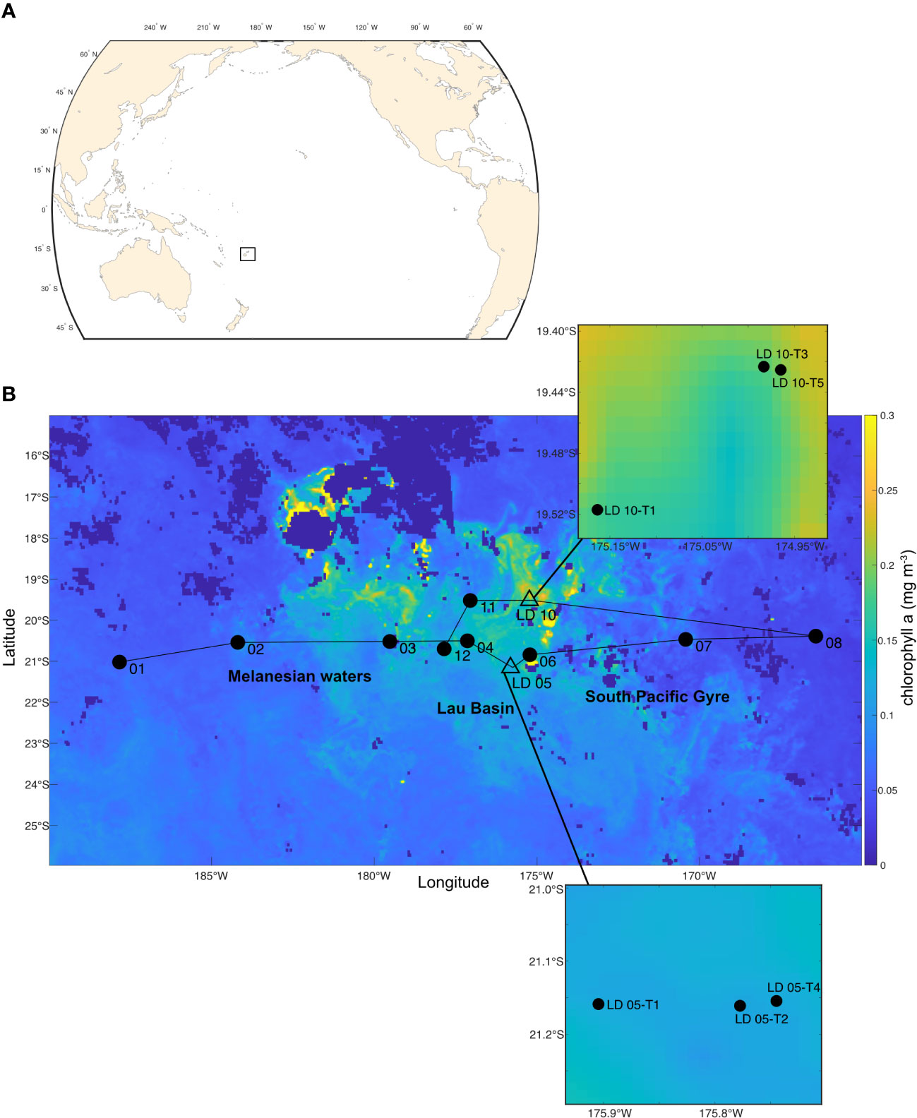
Figure 1 (A) Map of the Pacific Ocean showing the position of the Tonga Kermadec arc area by the black square. (B) Sampling map of the TONGA campaign superposed on the average chlorophyll a concentration ([Chl a]; mg m^-3) of November 2019 (data from MODIS-Aqua resolution of 4 km). Different oceanic regions were occupied during the cruise: Melanesian waters including short duration (SD) stations 01, 02 and 03, Lau Basin including SD 04, 11 and 12 as well as long duration (LD) stations 05 and 10, and the South Pacific Gyre including SD 06, 07 and 08. Zooms were performed on the substations with plankton sampling of the LD stations: LD 05-T1, -T2, and -T4 and LD 10-T1, -T3 and -T5.

Plankton was sampled during the day with WP2 nets of 200 μm and 35 μm mesh size, towed vertically from 0 to 200 m during simultaneous deployments. The 35 μm net was not deployed at SD 01 and both nets were not deployed at SD 09. Within the LD stations, plankton nets were deployed for substations LD 05-T1, -T2, and -T4, and LD 10-T1, -T3 and -T5. As the nets were not equipped with flowmeters, the filtered volumes were estimated by multiplying the net opening area (0.25 m²) by the length of cable unwound for each deployment (i.e. 200 m). This calculation potentially leads to an overestimation of the sampled volume since the possible backflow is not corrected (Heron, 1968). Samples from the 200 μm nets were directly concentrated onboard using a 100 μm sieve and preserved in a 4% formaldehyde solution. Samples from the 35 μm nets were separated into 5 subsamples for different analyses: the fraction intended for the present analysis was concentrated using a 20 μm sieve, preserved in acidic lugol solution and stored in opaque bottles. The 35 μm net sample from SD 02 was identified as potentially biased (abundance and size structure different by several orders of magnitude, symptomatic of an inconsistency in the sample subdivision strategy after collection) and was therefore excluded from our analysis.

2.2 Acquisition and treatment of plankton imaging data

2.2.1 FlowCam

The FlowCam analyzer imaging instrument (Fluid Imaging Technologies; Sieracki et al., 1998) equipped with a ×4 objective was used to study the micro-plankton samples (size range of 20-200 μm) from the 35 µm net at the Quantitative Imaging Platform (PIQv) of the Institut de la Mer de Villefranche. This instrument is an automated microscope taking digital images while microscopic particles are pumped through a capillary imaging chamber. Each sample was previously passed through a sieve of 200 μm to remove large objects which could clog the FlowCam imaging cell. Samples were then diluted or concentrated to achieve optimal object flow, and were run through a 300 μm deep glass cell. The auto-image mode was used to image the particles in the focal plane at a constant rate.

2.2.2 ZooScan

The ZooScan imaging instrument (Gorsky et al., 2010) was used to study the meso-plankton (> 200 μm). Samples from the 200 μm nets were gently filtered through 1000 μm and 100 μm mesh and transferred to filtered seawater. They were separated into two size classes: 200-1000 µm and > 1000 µm. Fractions were then split using a Motoda box (Motoda, 1959) to reach a concentration of approximately 1000 objects per subsample and scanned using the ZooScan. This sampling strategy allowed to consider correctly both the numerous small organisms and the large ones, which could be under-sampled if subsampled together by the Motoda box.

2.2.3 Image annotation

For both instruments, the full methodology used is displayed in their respective manual (https://sites.google.com/view/piqv/piqv-manuals/instruments-manuals). Briefly, images generated by the FlowCam and ZooScan were processed using the ZooProcess software (Gorsky et al., 2010) that extract segmented objects as vignettes, with a series of morphometric measurements that were imported into the EcoTaxa web platform (Picheral et al., 2017) for taxonomic classification. Using image recognition algorithms, predicted taxonomic categories were validated or corrected by a trained taxonomist. Overall, 51 406 vignettes were classified into 149 taxa for the ZooScan analyses, and 109 185 vignettes were classified into 124 taxa for the FlowCam analyses. For the majority, the taxonomic classification effort was possible up to the genus and only in rare cases up to the species. A number of organisms could not be reliably identified due to a lack of identification criteria and were therefore grouped into temporary categories (t00x) following similar morphological criteria.

2.2.4 Diazotrophs images

On the FlowCam vignettes, different morphologies of cyanobacteria were identified as diazotrophs, with sizes ranging between 20 and 200 μm. Among them were identified the cyanobacteria Katagnymene spiralis, free-living Richelia but also in symbiosis within Rhizosolenids diatoms (category Rhizosolenids inter-Richelia) and colonies of unicellular cyanobacteria (UCYN, allowing a sufficient size for detection by FlowCam imagery), likely corresponding to colonies of UCYN-B very abundant in this region (Bonnet et al., 2018; Stenegren et al., 2018). As the identification criteria are insufficient to reliably associate morphologies to genus, we grouped these cyanobacterial morphologies into morphotype categories named cyano a, cyano b and “t005_F”. On an identification basis of Tenório et al. (2018), the cyano a category could correspond to some Katagnymene species while cyano b could correspond to Trichodesmium but we chose to keep morpho groups as other authors, such as Lundgren et al. (2005), consider both morphotypes as Trichodesmium. We were also able to identify diazotrophic cyanobacteria on ZooScan vignettes (organisms > 200 μm): the cyanobacterium Katagnymene spiralis and a morphology group “cyanobacteria’’ probably corresponding to Trichodesmium species. Examples illustrating these diazotrophs vignettes and morphologies can be found in Figure 2 or directly in the open access project EcoTaxa: https://ecotaxa.obs-vlfr.fr/prj/2841 for the FlowCam and https://ecotaxa.obs-vlfr.fr/prj/2832 for the ZooScan.

FIGURE 2

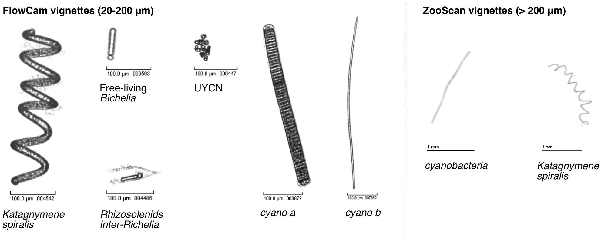
Figure 2 Examples of vignettes (FlowCam and ZooScan vignettes) for each category of organisms identified as diazotrophs. All of these categories were grouped into the functional plankton group ‘cyanobacteria’ for the 3rd analysis (see part 2.3 and 3.4).

2.3 Numerical and statistical analysis

Using a custom-made processing tool (https://github.com/ecotaxa/ecotaxatoolbox), the data were structured in two distinct databases (ZooScan and FlowCam). Major and minor axes of the best ellipsoidal approximation were used to estimate the biovolume (mm³ m^-3) of each object according to the recommendation of Vandromme et al. (2012). Size was expressed as equivalent spherical diameter (ESD, μm). The individual biovolumes of the organisms were arranged in Normalized Biomass Size Spectra (NBSS) as described by Platt (1978) along a harmonic range of biovolume so that the minimal and maximal biovolumes of each class be linked by: Bv_max= 2^0.25 Bv_min. The NBSS was obtained by dividing the total biovolume of each size class by its biovolume interval (Bv_range=Bv_max-Bv_min). The NBSS was representative of the number of organisms (abundance within one factor) per size class. This can provides insight into ecosystem structure and function through the “size spectra” approach, which generalizes Elton’s pyramid of numbers (Elton, 1927). For each database, considering the volumes of water filtered by the nets, plankton concentration in individu per m^-3 (ind m^-3) and biovolume were calculated for each taxonomic annotation and for several levels of grouping: living or non-living, and a functional group annotation. Fifteen planktonic functional groups were defined. The full list of functional group annotations linked with their EcoTaxa taxonomic label can be found in Supplementary Table 1. Diversity was calculated with the Shannon Index (H).

Hierarchical clustering analyses (HAC; descriptive complete link method, Hellinger distance; Legendre and Legendre, 2012) were performed on the relative abundance to group stations with similar planktonic compositions. Principal component analysis (PCA) was performed on the relative abundance (Hellinger transformation; Legendre and Legendre, 2012) of all taxonomic annotations. To link both analyses, the groupings obtained in the HAC analysis were reprojected into the PCA space. The addition of environmental data (temperature, salinity, oxygen, nitrite: NO_2, nitrate: NO₃^-, ammonium: NH₄, phosphate: PO₄^3-, dissolved iron: DFe, particulate iron: Pfe, silicate: Si(OH)₄, manganese: Mn, aluminum: Al and fluorescence; see part 2.4) as supplementary data was performed in the PCA, allowing to cross-link the environmental influence with the taxonomic composition of the station. Spearman correlation tests were performed between different variables (alpha risk set at 0.05%).

2.4 Plankton adjustment and assembling

In order to study the whole community (all planktonic organisms > 20 μm), we merged the two databases (FlowCam and ZooScan) into one single cross-calibrated database. In its lowest size range, each dataset from FlowCam and ZooScan displayed an undersampling which is symptomatic of either incorrect detection of objects due to optical limitation of device or undersampling of net by mesh extrusion of organisms (Figure 3A; Lombard et al., 2019). Therefore, all parts of the NBSS below the maximal abundance of each device were discarded (Figure 3B). For the highest size range of each dataset, very large organisms were associated with a presence-absence signal rather than a quantitative concentration due to insufficient sampling effort, and were disregarded (Figure 3B). We chose as an objective criterion to discard every NBSS size bin separated by more than five empty size bins. A clear difference of intercepts between NBSS spectra of the two instruments was detected (Figure 3B). Using the ZooScan as a reference, we used overlapping observations between the two instruments (for overlapping observations of size classes 1 to i) at a given station j to produce a cross-size classes average correction coefficient at the station scale such as: NBSS _{FlowCam adjusted j} = NBSS _{FlowCam j} × mean (NBSS _{FlowCam ij/}NBSS _{ZooScan ij}). Results of this correction are shown in Figure 3C.

FIGURE 3

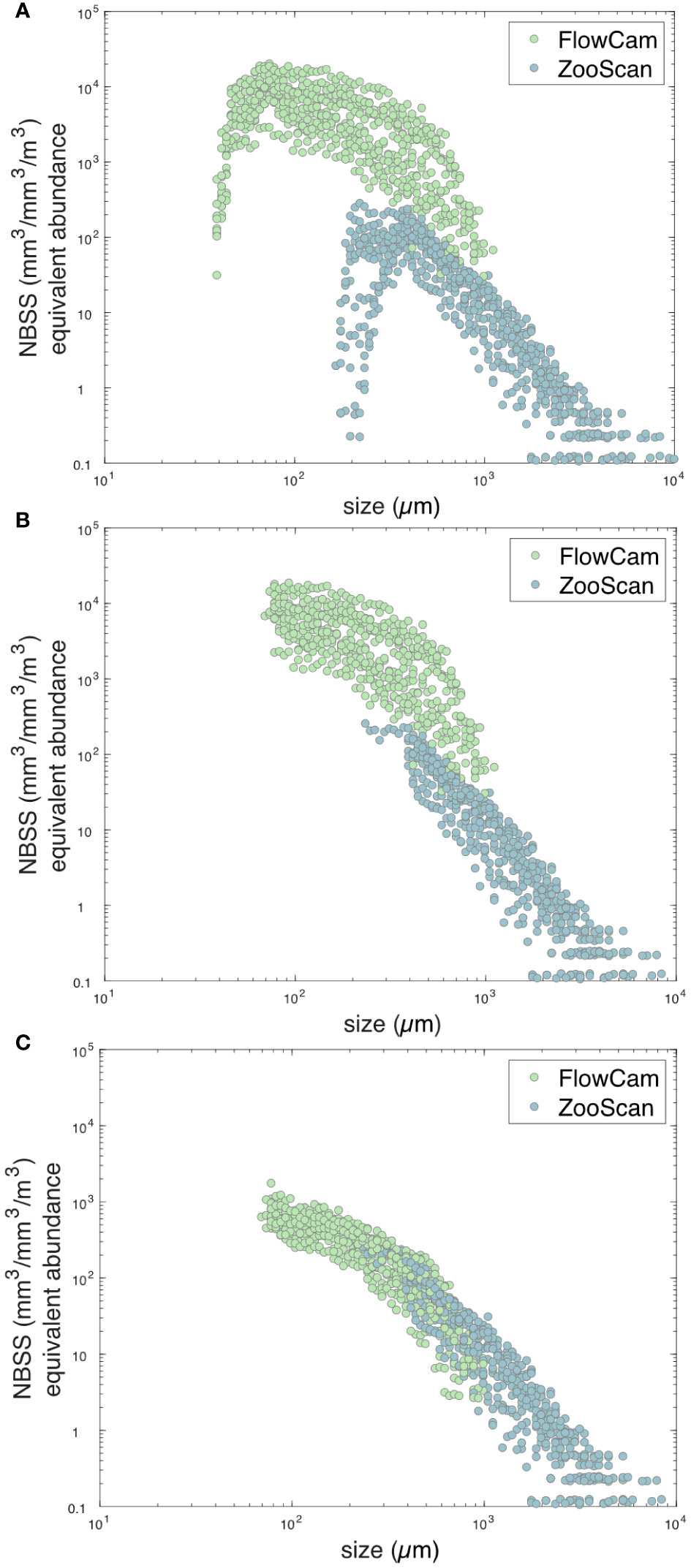
Figure 3 Normalized Biovolume Size Spectra (NBSS) in mm^-3 m^-3 representative of the number of living organisms per size class (μm) imaged with the two different quantitative imaging devices: FlowCam and ZooScan. (A) NBSS representation of the raw data before the correction methods. (B) NBSS representation of the intermediate data with the correction of the undersampling in the lowest and largest class size. (C) NBSS representation of the adjusted data with the application of the cross-size class average correction coefficient (ZooScan was used as a reference).

Finally, to have a unique dataset in the overlapping size range, an average between the values of NBSS _{FlowCam adjusted i,j} and NBSS _{ZooScan i,j} was performed for each station at the functional and trophic group levels. From these unique NBSS spectra, concentrations and biovolumes were calculated. A non-negligible risk to duplicate counts of organisms exists at the original taxonomic identification level, which may differ in taxonomical resolutions between instruments. For example, while different morphotypes of cyanobacteria can be identified with the FlowCam, they are only identified at the level of the phylum cyanobacteria with the ZooScan. To avoid this, assembly at the initial taxonomic identification level was not used, and was only done at functional and trophic levels. We performed a HAC on the normalized biovolume (square root transformation) to group together stations with similar functional planktonic groups. PCA was performed on the normalized biovolume of functional planktonic groups. To link the two analyses, the groupings obtained in the HAC analysis were reprojected into the PCA space. The association with the environment was tested by adding environmental variables as supplementary variables in the analysis and evaluating their correlations to the PCA components. For all linear relationships, we used a robust linear fit which is less sensitive to potential outliers (Greco et al., 2019).

2.5 Environmental data

Temperature, conductivity (salinity), pressure (depth) and dissolved oxygen vertical profiles were obtained using a rosette-mounted CTD SBE 9 plus sensor (data available on SEANOE: https://doi.org/10.17882/88169). At each station, conventional CTD casts were conducted to sample inorganic nutrients using a rosette equipped with 24 Niskin bottles (12 L) and Trace-Metal clean Rosette (TMR) casts were performed for dissolved and particulate trace metal sampling. Seawater samples were collected according to the GEOTRACES guidelines using a Titanium rosette equipped with 24 Teflon-coated 12-L Go-Flos bottles (General Oceanics) and operated along a Kevlar cable. The cleaning protocols for sampling bottles and equipment also followed the GEOTRACES Cookbook (Cutter et al., 2017). CTD and TMC profiles showed a difference in calibration for the O₂ sensors. A linear regression was performed using a robust method (Greco et al., 2019) to adjust the TMC profiles to the quality controlled CTD profiles.

2.5.1 Dfe data

[DFe] was measured from TMR casts by flow injection with online preconcentration and chemiluminescence detection. Each sample was analyzed in triplicate and following GEOTRACES recommendations for validation. Full protocol and dataset can be found in Tilliette et al. (2022).

2.5.2 Nutrients

Inorganic nutrients (NO_2, NO₃^-, PO₄^3- and Si(OH)₄) were measured as detailed in Bonnet et al. (2018): 20 mL of filtered water samples were collected into High Density PolyEthylene (HDPE) flasks. Filtration by gravity was done through a Sartobrand cartridge from each CTD niskin. NO₂, NO₃^- and PO₄^3- samples were frozen at -20°C while Si(OH)₄ samples were only refrigerated pending analysis. For ammonium (NH₄), 20 mL samples were collected into PC 60 mL Nalgene Oak Ridge bottles. Analysis was performed on board using a Fluorimeter TD-700 Turner Designs using Holmes et al. (1999) method.

2.5.3 Particulate trace elements

Trace element measurements were carried out within 12 months of collection by a SF-HR-ICP-MS Element XR instrument (Thermo Fisher, Bremen, Germany), at Pôle Spectrométrie Océan (IFREMER, France). The method employed was similar to that of Planquette and Sherrell (2012). Particulate Mn (pMn), pFe and pAl were used as proxies to trace hydrothermal inputs.

2.5.4 Interpolation of environmental data

Data were interpolated on the vertical dimension to have a regular depth step (one value every meter from 0 to 200 m) and thus make the dataset homogeneous to reduce the sampling bias. Macronutrients (NH₄, NO₃^-, PO₄^3- and Si(OH)₄), DFe and pTM data were polynomially interpolated with a fourth order polynomial function (1), while NO₂ data were interpolated following the Gaussian Model (2):

$\begin{array}{ll}f(x) : x^{4}p1+x^{3}p2+x^{2}p3+x^{1}p4 + p5& (1)\end{array}$

$\begin{array}{ll}f(x)= a1 \times e^{-{((x-b1)/c1)}^2}& (2)\end{array}$

Because macronutrients, DFe and pTM were generally not collected above 10 m, the surface reference depth was set at 10 m. This also avoids much of the strong variability due to the diurnal cycle in the upper ocean. For all interpolation with a fourth order polynomial function, an upper bound was imposed by setting the deepest concentration value to 200 m. For each station, the Mixed Layer Depth (MLD) has been calculated as the depth where θ = θ_10m ± 0,2°C (de Boyer Montégut, 2004). The MLD ranged from minimum 17 m (SD 07) to maximum 71 m (SD 03). Two values were finally calculated per environmental parameter by averaging the interpolated data from the surface to the MLD (data “up”) and then from the MLD to 200 m (data “down”). The DCM was estimated as the depth at which fluorescence (proxy for Chl a) is maximum, according to Sauzède et al. (2015).

2.6 Acoustic data: indicator of macro-zooplankton biomass and density

Continuous acoustic measurements were made with a calibrated (Foote, 1987) Simrad EK60 echosounder operating at two frequencies: 38 and 200 kHz. To focus on the acoustic scattering in the photic layer, we only used the 200 kHz frequency, with a maximum acquisition range of 120 m. Power and pulse length were 45 W and 1024 μs, respectively. Data used in this study were acquired with an average ping interval of 7 s when the vessel speed was higher than 2 knots. Acoustic data were scrutinized, corrected and analyzed using the “Movies3D” software developed at the Institut Français de Recherche pour l’Exploitation de la Mer (Ifremer; Trenkel et al., 2009) combined with the French open-source tool “Matecho” (Perrot et al., 2018) from the Institut de Recherche pour le Développement (IRD). Noise from the surface was removed (from 3 m below the transducer, i.e. 8 m depth from the surface), the bottom ghost echoes were excluded, and the bottom line was corrected. Single-ping interferences from electrical noise or other acoustic instruments, and periods with either noise or attenuated signal due to inclement weather were removed using the filters described by Ryan et al. (2015). Background noise was estimated and subtracted using methods described by de Robertis and Higginbottom (2007). The nautical area scattering coefficient (NASC in m² nmi^-2), an indicator of marine organism biomass, and the volume backscattering strength (Sv in dB re 1 m^-1), an indicator of the marine organism density, were calculated. Acoustic symbols and units used here follow Maclennan (2002). Data were echo-integrated into 1 m high layers over a 0.1 nm giving one ESU (Elementary Sampling Unit) with a -100 dB threshold from 8 m down to 120 m depth. Diel vertical migration (DVM) is a common behavior for zooplankton and micro-nekton that can be observed at almost all spatial scales (Haury et al., 1978). Acoustic data were thus split into day, night and crepuscular periods (dawn and dusk). Day and night periods were defined based on the solar elevation angle: daytime when the solar elevation is higher than 18° and night when the solar elevation is lower than 18°, as described in Lehodey et al. (2015).

2.7 Lagrangian analysis

2.7.1 Velocity currents and trajectories calculation

Horizontal current velocities were provided by the Copernicus Marine Environment Monitoring Service (CMEMS, http://marine.copernicus.eu/). These are considered representative of the velocities in the first ~50 m of the water column, include a geostrophic and Ekman components, and have a daily resolution and 1/25° spatial resolution (product SEALEVEL_GLO_PHY_L4_REP_OBSERVATIONS_008_047). Trajectories were calculated with a 3 hours time step, using a Runge-Kutta scheme of order 4.

2.7.2 Chlorophyll a data

Chlorophyll [CHL a] data were obtained from the OCEANCOLOUR_GLO_BGC_L4_MY_009_104-TDS product which was provided by CMEMS platform (product version cmems_obs-oc_glo_bgc-plankton_my_l4-gapfree-multi-4km_P1D). This is satellite product of level 4 with 4 km spatial resolution and is provided daily. Daily fields of [CHL a] for the month of November 2019 were averaged together, providing the mean [CHL a] of our region of interest during the campaign period.

2.7.3 Detection of the lagrangian plume stemming from the 2 target volcanoes

In order to quantify the effect of the Tonga Arc on phytoplankton concentration, we analyzed whether water parcels displaying enhanced [Chl a] had been in contact with the two shallow hydrothermal vents. To achieve this, a regular grid of 0.1° cell-size (~11 km) covering the study region was created. Each point, considered representative of a water parcel, was advected backward in time from a day t₀ until t₀-150 days. Then, for each water parcel, we identified how many days before it eventually passed over one of the two volcanoes (considered as a disk of 0.5° (~55 km) radius). This metric, hereafter the Lagrangian plume, was calculated using the 1^st of November 2019 as t₀. This operation was repeated for each day between the 1^st and the 30^th of November 2019, and the 30 Lagrangian plume fields were averaged together. Points that did not come into contact with either volcano were excluded from the average. The two volcanoes were considered in correspondence with LD 10-T5 and LD 05-T4, which were the closest stations to the hydrothermal vents. This approach has already been validated to study the island mass effect, and has made it possible to reproduce the Kerguelen and Crozet blooms (Sanial et al., 2014; d’Ovidio et al., 2015; Sanial et al., 2015) or, more recently, the phytoplankton bloom stemming from seamounts in the Southern Ocean (Sergi et al., 2020).

2.7.4 Bootstrap test

A bootstrap test was performed to test whether water parcels which came into contact with the volcanoes, and the water parcels which did not, presented different [CHL a] values. For this purpose, firstly we calculated the [Chl a] value for each point of the regular grid (using the mean [Chl a] of November 2019). Secondly, we divided the grid points into two groups: those which have been in contact with volcanoes, less than τ days before, and those who did not. The statistical independence of the two groups was tested with a Mann-Whytney or U test. Finally, a bootstrap analysis was applied following the methodologies in Baudena et al. (2021). As τ, we tested different values, ranging from 5 to 150 days. We selected a tau of 115 days because it was the greatest value for which the difference between the two groups was significant.

3 Results

3.1 Environmental characteristics

The Melanesian waters and the South Pacific Gyre were characterized by oligotrophic waters ([Chl a]< 0.15 mg m^-3; Figure 1; DCM: 100-180 m). In contrast, the Lau Basin was characterized by mesotrophic waters in the vicinity of the Tonga arc ([Chl a] > 0.15 mg m^-3; Figure 1; DCM: 70-90 m). NO₃^- concentrations at the surface (0-50 m) were consistently close or below the detection limit (0.05 μmol L^-1) throughout the transect, while PO₄^3- concentrations were typically 0.1 μmol L^-1 in oligotrophic zones and depleted down to detection limit (0.05 μmol L^-1) in the mesotrophic zone (i.e. Lau Basin). Concerning the dFe values (Tilliette et al., 2022), stations furthest from the Tonga-Kermadec arc in the South Pacific Gyre (i.e., SD 7 and 8) were characterized by low [dFe] in the photic layer (< 0.2 nmol kg^-1). The station SD 6, closest to the arc was slightly different from the other stations of the gyre. Although [dFe] remain low throughout the whole water column (< 0.3-0.4 nmol kg^-1, [dFe] were higher than those at SD 7 and 8 in the surface layer. Melanesian waters were characterized by a dFe enrichment in the photic layer compared to the waters of the South Pacific gyre with [dFe] as high as 0.4-0.5 nmol kg^-1. In the Lau Basin, we observed higher [dFe] than in the South Pacific gyre as well as in Melanesian waters for all stations. SD 11 had the highest [dFe] of the SD in the Lau Basin in the photic layer (0.4-0.6 nmol kg^-1). SD 12 presented the least enriched photic layer, with [dFe] similar to those observed to the east (~0.2 nmol kg^-1). Sea surface temperature (SST) ranged from 24.3°C (SD 01) to 27.3°C (LD 10-T3) above the MLD.

3.2 Description of the micro-plankton community (20-200 μm)

3.2.1 Quantification

The highest micro-plankton concentrations were found at stations west of the Tonga arc, reaching a maximum at SD 11 (8.60 10⁴ ind m^-3), LD 10-T5 and LD 10-T3, followed by LD 05-T1 and LD 05-T2 (Figure 4A). The minimum of micro-plankton abundance was found in SD 06 (8.75 10³ ind m^-3) located right to the east of the Tonga Arc. The average concentration of micro-plankton in the Lau Basin was 4.33 10⁴ ind m^-3. Micro-plankton concentrations in the South Pacific Gyre were 2.28 times lower on average (1.90 10⁴ ind m^-3).

FIGURE 4

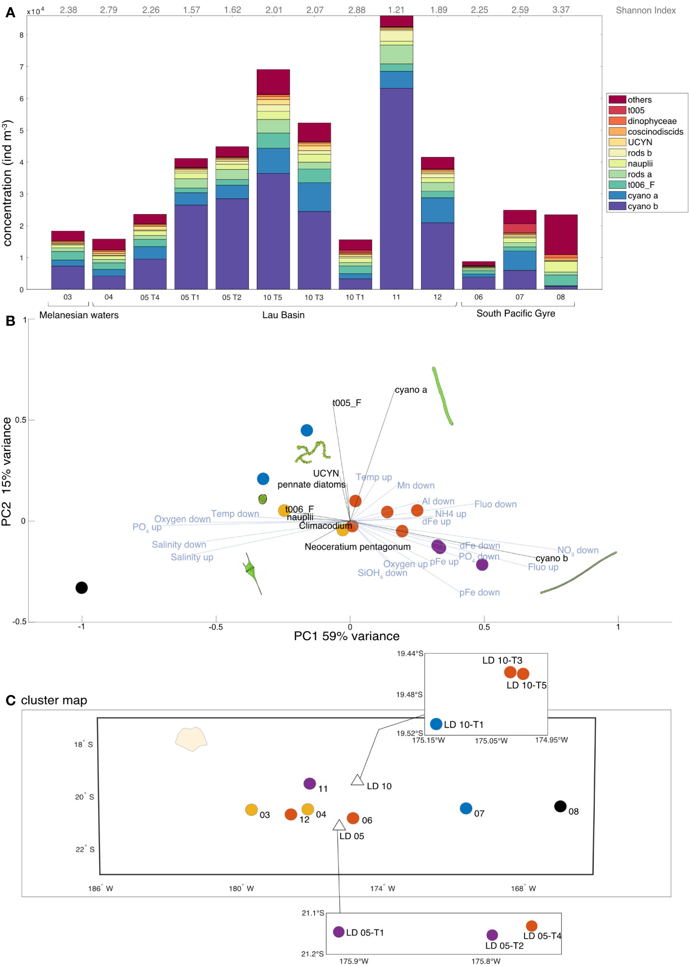
Figure 4 (A) Micro-plankton concentration (ind m^-3) and composition of the 10 most abundant taxa (representing about 88% of the dataset). The rest of the micro-planktonic organisms (114 taxa) were grouped within the category “others”. Values of the Shannon diversity Index are indicated in grey. (B) Principal Component Analysis (PCA) on relative abundances of micro-plankton (Hellinger-transformed data). Only environmental data (in blue) with a contribution greater than 0.25 and taxonomic data (in black) with a contribution greater than 0.18 are shown for ease of reading. The environmental variables are the averages of interpolated data from the surface to the MLD (up) and then from the MLD to 200 m (down). The colors correspond to the five characteristic clusters determined via an independent hierarchical analysis (HAC) with Euclidean distance. (C) Projection of the clusters determined by HAC on the transect map with the corresponding station numbers. Credit plankton illustration: Tohora Ereere.

3.2.2 Community composition

In terms of community composition, diazotrophic cyanobacteria clearly dominated, notably cyano a and b, UCYN colonies and t005_F, accounting for 69% on average of the total micro-planktonic concentration (total: 5.00 10⁵ ind m^-3), with a maximum at SD 11 (80% of the total community). This dominance was confirmed by the linear regression between cyanobacteria and total micro-plankton concentration (R2 = 0.92). Furthermore, a significant negative correlation was found between the micro-plankton concentration and the Shannon diversity Index (data not shown; y = 1.72 10^-5 x + 3.17; R² = -0.72, p = 0.007). The majority of the variance in the PCA (Figure 4B; PC1; 59% of variance) showed that the diazotroph dominance correlated with water rich in DFe, Chl a and pTM (pAl and pMn), and low salinity and PO₄^3- concentrations. Changes in community correlated to [DFe] were observed. First, a community dominated by cyano b (probably genus Trichodesmium) correlated to high [DFe] was found. Secondly, cyano a and t005_F (probably genus Katagnymene for both) were associated to UCYN. Then, a cyanobacteria-poor community was correlated with low [DFe]. Diazotrophic cyanobacteria-poor stations had a more diverse micro-plankton community, such as at SD 08 in the South Pacific Gyre which differed strongly from other stations. Even if this difference represents a few percentages of variance (Figure 4B; PC2; 15%), different cyanobacteria distribution was found in the Lau Basin notably between the two LD stations. More cyano a and t005_F (Katagnymene) were found at LD 10 while more cyano b (Trichodesmium) were measured at LD 05. This can also be seen on the cluster map (Figure 4C), with stations close to the Tonga arc showing clusters characterized by cyanobacteria dominance, except for LD 10-T1 which is associated with SD 07 in the South Pacific Gyre.

3.3 Description of the meso-plankton community (>200 μm)

3.3.1 Quantification

The highest meso-plankton concentrations (Figure 5A) were found in the Lau Basin at LD 10-T5 (510.6 ind m^-3), followed by LD 10-T3 station (446.0 ind m^-3) then by LD 05 sub-stations and at SD 11 and 12. The average concentration in the Lau Basin was 328.9 ind m^-3. In contrast, low concentrations were found in the oligotrophic zone of the South Pacific Gyre, with SD 07 (78.6 ind m^-3) and SD 08 (112.7 ind m^-3). The mean concentration in the South Pacific Gyre was 132.8 ind m^-3, while Melanesian waters showed an intermediate mean meso-plankton concentration of 232.6 ind m^-3. Contrary to the micro-plankton where the concentration was negatively correlated to the diversity (cyanobacteria dominance opposed to a diverse community), no significant correlation was found between meso-plankton concentration and the Shannon diversity Index (data not shown; y = - 8.20 x 10-4 + 3.12; R2 = 0.51; p = 0.06). The relative abundances underlined a shift from copepod dominance to co-dominance of cyanobacteria and copepods (or over-dominance of cyanobacteria in some cases) west of the Tonga arc as one approaches the arc.

FIGURE 5

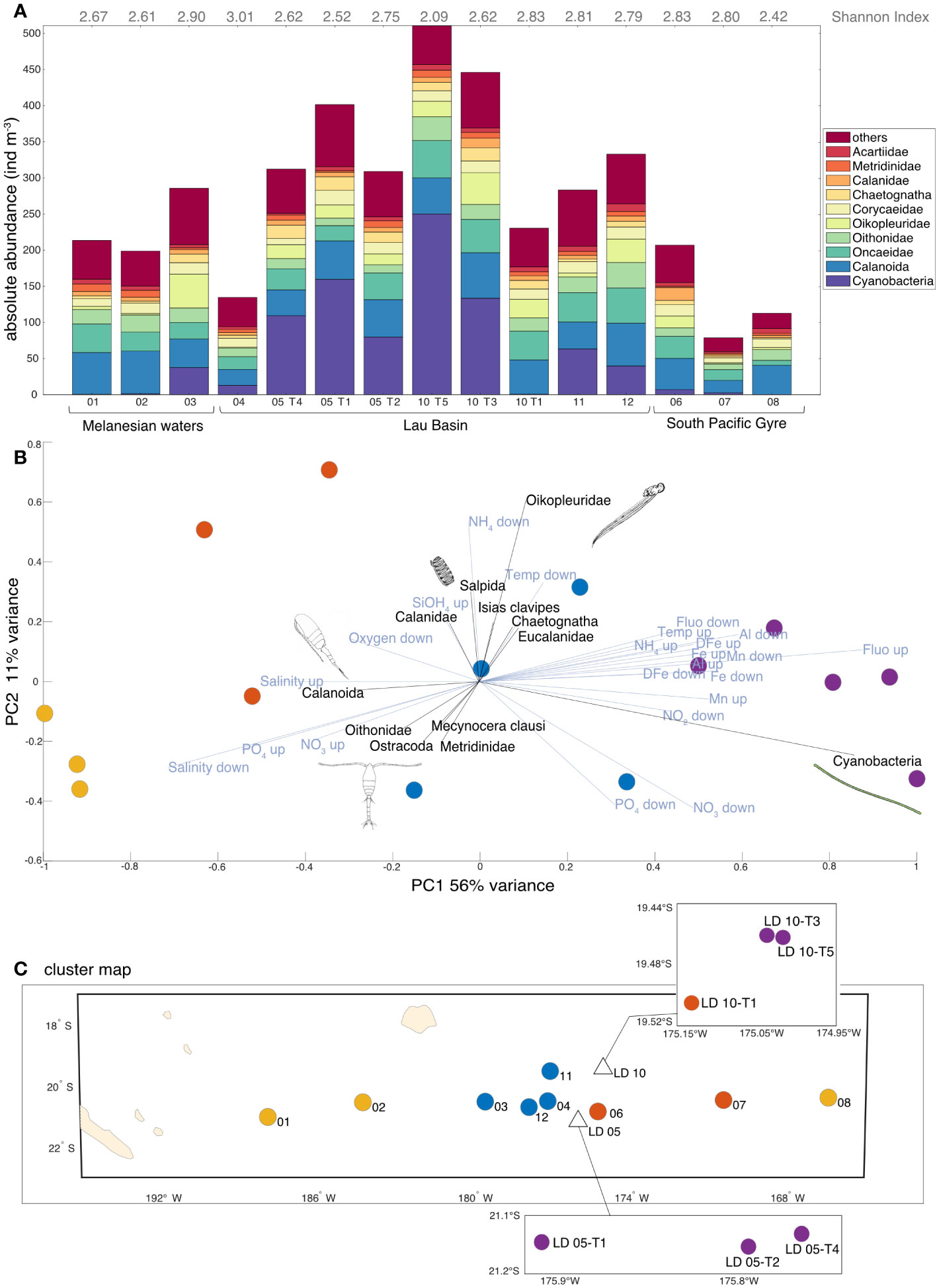
Figure 5 (A) Meso-plankton concentration and composition of the 10 most abundant groups (representing about 79% of the dataset). The rest of the planktonic organisms (139 taxa) are grouped within the category “others”. Values of the Shannon Index diversity are indicated in grey. (B) Principal Component Analysis (PCA) on relative abundances of meso-plankton (Hellinger-transformed data). Only environmental data (in blue) with a contribution greater than 0.25 and taxonomic data (in black) with a contribution greater than 0.17 are shown for ease of reading. The colors correspond to the four characteristic clusters determined via an independent hierarchical analysis (HAC) with Euclidean distance. The environmental variables are the averages of interpolated data from the surface to the MLD (up) and then from the MLD to 200 m (down). (C) Projection of the clusters determined by HAC on the transect map with the corresponding station numbers. Credit plankton illustration: Tohora Ereere.

3.3.2 Community composition

PCA coupled with cluster analysis (Figures 5B, C) showed a very strong signal on meso-planktonic community change. The maximum of the variance (PC1: 56% of variance; Figure 5B) showed a clear gradient, with (i) the more diverse communities dominated by different copepod genus within SD far from the Tonga Arc (SD 08, 01, 02); (ii) distinctive communities in SD 06, 07 and LD 10-T1, (iii) communities with a rather gelatinous composition (i.e. salpida, oikopleura, chaetognatha, generally filter-feeding and detritivorous organisms) at most SD of the Lau Basin, and (iv) cyanobacteria-dominated communities at LD sub-stations close to the Tonga Arc. Cyanobacteria-dominated sub-stations were correlated with waters rich in DFe, Chl a and pTM (pAl and pMn), but with low salinity and PO₄^3-.

3.4 Description of the plankton community as a whole

3.4.1 Quantification

To consider both micro- and meso-plankton equally, we considered their biovolume (proxy for biomass) rather than their concentration. An increase in plankton biovolume (Figure 6A) was observed in the Lau Basin with the highest biovolumes observed at LD 10-T3 and LD 05-T1 (i.e. 100.15 and 94.98 mm³ m^-3, respectively). The mean biovolume in the Lau Basin was 66.44 mm³ m^-3 while the mean biovolume in the South Pacific Gyre was 35.64 mm³ m^-3. The lowest planktonic biovolumes were found in these oligotrophic waters, especially at SD 07 and 08 where biovolumes reached values of 13.32 and 16.32 mm³ m^-3, respectively.

FIGURE 6

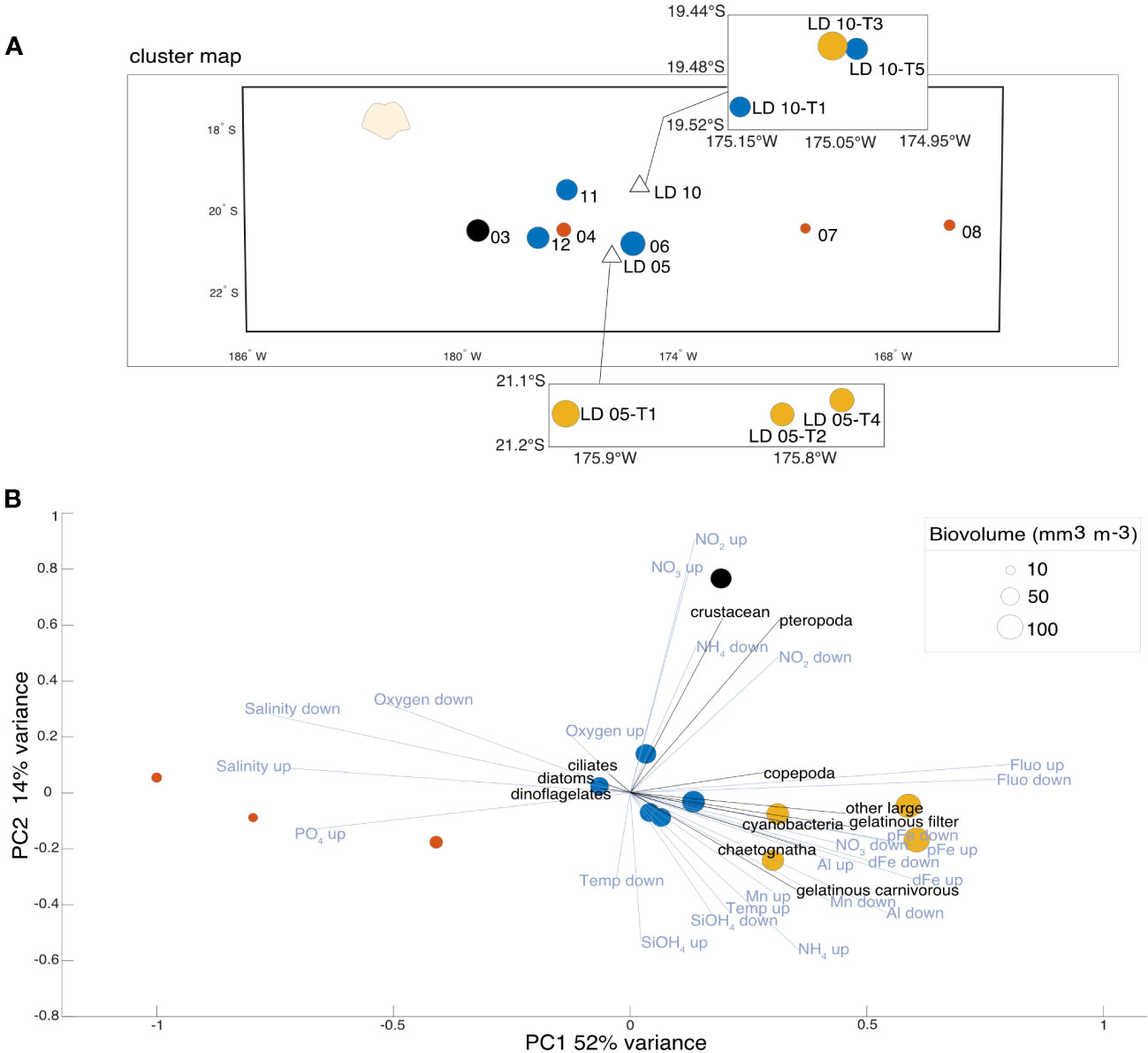
Figure 6 (A) Projection of the clusters determined by hierarchical analysis (HAC) on the transect map with the corresponding station numbers, points size corresponding to biovolume. (B) PCA on normalized biovolume (equivalent to biomass) of the plankton functional types (pft; in black). Only environmental data (in blue) with a contribution greater than 0.25 are shown for ease of reading. The environmental variables are the averages of interpolated data from the surface to the MLD (up) and then from the MLD to 200 m (down). The size corresponds to the plankton biovolume (mm³ mm^-3) at each station. The colors correspond to the four characteristic clusters determined via the hierarchical analysis (HAC) with Euclidean distance.

3.4.2 Community composition

The planktonic community identified at SD 04, in the Lau Basin, was similar to those measured in the stations in the gyre, reaching a low biovolume (26.31 mm³ m^-3; Figures 6A, B). The PCA (Figure 6B) described a plankton community dominated by cyanobacteria associated with gelatinous organisms (pft: filter feeders, carnivores and chaetognatha) and directly correlated with waters rich in DFe, Chl a and pTM (pAl and pMn) but with low salinity and PO₄^3-. The cyanobacteria-dominated community, associated in previous analyses with LD stations, appears from this analysis to be more representative of LD 05. Indeed, two of the three LD 10 substations were associated with the more diverse planktonic communities in the Lau Basin by the clustering analysis. SD 03, located in the Melanesian waters, is distinguished from the other stations by its high crustacean and pteropod biovolume correlated with high surface NO₃^- concentrations. The oligotrophic zone of the South Pacific Gyre is composed of a community dominated by small autotrophs (pft: ciliates, diatoms, and dinoflagellates).

3.5 Impact on the higher food web (macro-zooplankton and fish) with acoustic detection

Acoustic detection analysis was carried out to gain an overview of the upper food web, mainly meso- and macro-zooplankton. To this end, we represented the results of acoustic detection during the cruise trajectory, with an indicator of the density of these organisms (Sv) in Figure 7A and an indicator of their biomass (NASC) in Figure 7B. The oligotrophic waters of the South Pacific Gyre were identified as poor in biomass and density of meso-plankton and fish (i.e minimum NASC of 5.60 m² nmi^-2 at 167°W in the South Pacific Gyre; Figure 7B). A clear progressive increase in biomass towards the Lau Basin was observed. A biomass peak (up to NASC of 7.40 m² nmi^-2 at 177°W; Figure 7B) was observed in the Lau Basin near the Tonga Arc where the maximum plankton biomass was also observed (see sections 3.2, 3.3 and 3.4). A slight decrease in biomass (NASC average of 6.52 ± 3.32 m² nmi^-2 from 180°W to 193°W; Figure 7B) was visible in the Melanesian waters compared to the Lau Basin, although it was still higher than the biomass observed in the South Pacific Gyre.

FIGURE 7

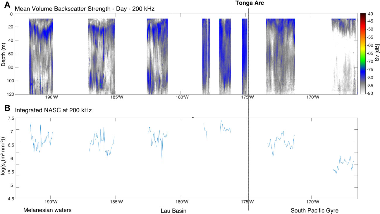
Figure 7 (A) Synthetic averaged acoustic density (Sv) echogram at 200 kHz from 8 to 120 m during the day. Color bar indicates Sv in dB re 1 m^-1. The organisms observed by these acoustic methods are mainly macro-zooplankton and fish. (B) Integrated acoustic biomass (nautical area scattering coefficient NASC in log(s_A(m² nmi^-2)) at 200 m. The Sv and NASC are averaged on a 0.05° longitude step grid. For (A) and (B), the approximate position (Ruellan and Lagabrielle, 2005) of the Tonga arc is represented by a black dotted line.

3.6 Lagrangian dispersion around the two target hydrothermal vents of the Tonga Arc

The Lagrangian plume, averaged over the month of November 2019, reveals a global dispersion towards the southeast (Figure 8A). The water parcels sampled at SD 06 (i.e. South Pacific Gyre), 11, 12 and 04 (i.e. Lau Basin) passed above the hydrothermal vents 35, 106, 114, and 103 days before the sampling, respectively. Conversely, water parcels sampled in the western oligotrophic Gyre (SD 08 and 09) and Melanesian waters (SD 01, 02 and 03) did not pass above the hydrothermal vents in the previous 115 days (see 2.7). To determine whether the hydrothermal vents affected the primary productivity of the region, the Lagrangian plume contour at 115 days was superposed on the mean [Chl a] of November 2019, finding a remarkable agreement (Figure 8B). For instance, a meander at around 22°S, 167°W characterized by an enhanced [Chl a] concentration, passed over the vents ~100 days before. To quantify whether the observed differences in Chl a content inside and outside the Lagrangian plume contour were significant, we performed a bootstrap test (Figure 8C) over the whole region. The test revealed that the [Chl a] was significantly higher inside the Lagragian plume (0.1044 mg m^-3) than outside (0.0738 mg m^-3; Figure 8C). Notably, we obtained a significant decrease in [Chl a] content as a function of the amount of time since the water parcel passed over the volcanoes (R² = 0.49, p< 0.05, slope: -0.0027 mg m^-3 d^-1; see Supplementary Figure 1). In other words, as water parcels moved away from the hydrothermal vents, their [Chl a] content decreased. The area of the 115-day Lagrangian influence patch is equal to 412 770 km² (white dashed surface air: Figures 8A, B). Complementing our results, previous and subsequent years (averaged over the month of November 2017, 2018, 2020 and 2021, see Supplementary Figure 2) also show an overall southeastward dispersion of Chl a, similar with our study year.

FIGURE 8

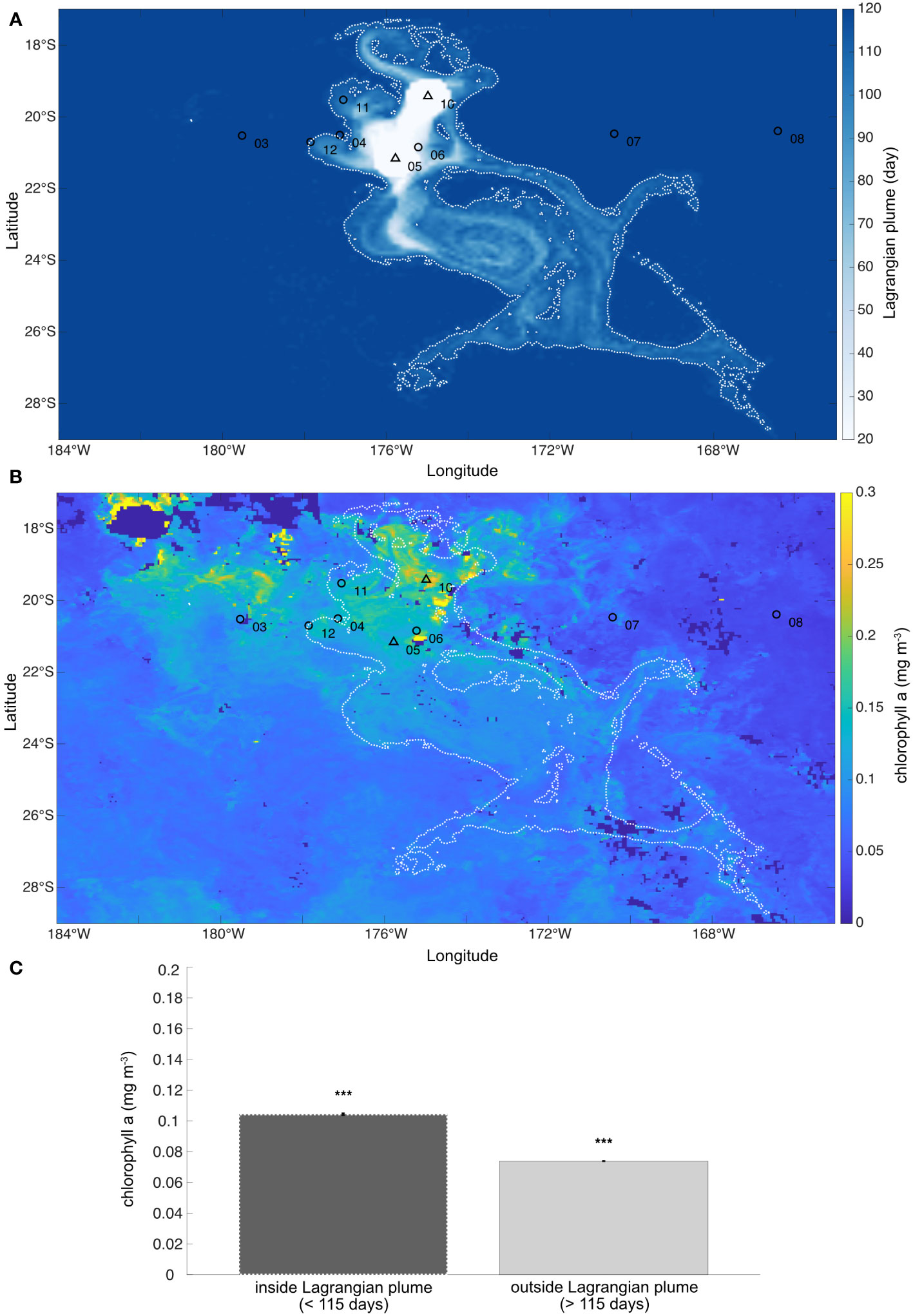
Figure 8 (A) Average Lagrangian plume for November 2019 in the WTSP region. The color of each point indicates how many days before the corresponding water parcel came into contact with one of the two target hydrothermal vents (black triangles). White dashed lines show the contours of the Lagrangian plume at 115 days. (B) Average chlorophyll a concentration ([Chl a]; mg m^-3) observed in November 2019 (monthly-mean composite image, data from MODIS-Aqua at 4 km resolution). White dashed lines show the contours of the Lagrangian plume at 115 days reported in panel (A). (C) Bootstrap results. The dark gray column shows the average [Chl a] inside the Lagrangian plume, i.e. at the locations showing a Lagrangian plume value less than 115 days, considered under the effect of the hydrothermal sources. Conversely, the light gray column shows the average [Chl a] outside the Lagrangian plume, i.e. at the locations showing a Lagrangian plume value greater than 115 days, considered as not affected by hydrothermalism. Error bars indicate the standard deviation. The three stars indicate the significance of the bootstrap test (p< 0.001) between the [Chl a] values inside and outside the Lagrangian plume.

4 Discussion

The main goal of the TONGA project was to evaluate the potential impact of shallow hydrothermal inputs in the vicinity of the Tonga volcanic arc on planktonic communities and organic carbon export to the deep ocean (Bonnet et al., 2023). This study highlights that plankton communities, from micro- to macro-plankton, harbor high abundances and biomasses in the Lau Basin located close to the Tonga volcanic arc and, to a lesser extent, in Melanesian waters located west of the arc (Figure 9). These high abundances and biomasses were correlated with the environmental signatures indicative of the hydrothermal vents, as indicated by Guieu et al. (2018) and Bonnet et al. (2023): waters rich in DFe, Chl a and particulate trace element (pAl and pMn) but low in salinity and PO₄^3- (see PCA Figures 4–6). Therefore, they are associated with these hydrothermal vents in a good agreement with Bonnet et al. (2023) who demonstrated that Fe-rich fluids released close to the shallow volcano represent a significant Fe source for planktonic communities in surface waters.

FIGURE 9

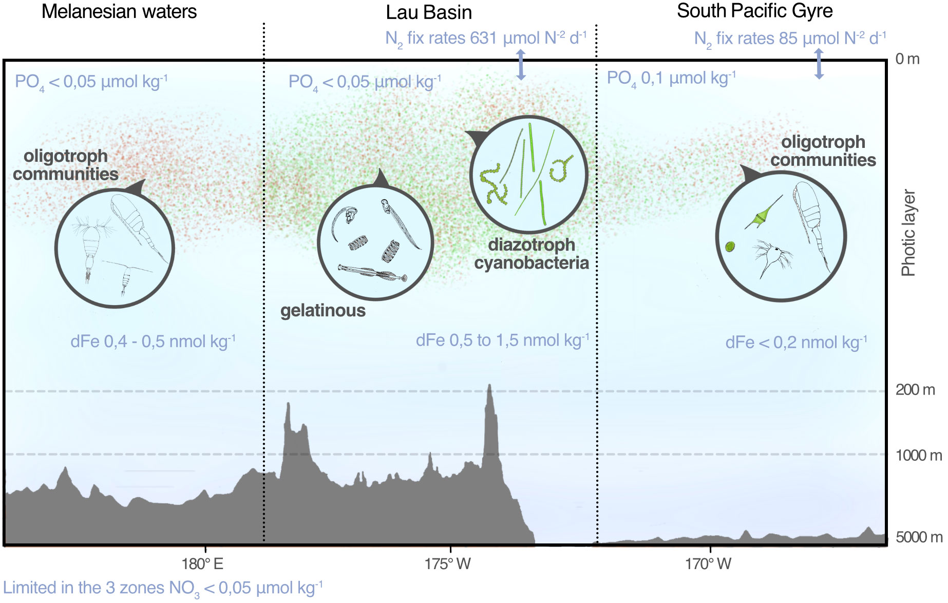
Figure 9 Summary diagram of the study results. The green and pink clouds represent the order of magnitude of the abundances of micro-plankton and meso-plankton, respectively (see Figures 3 and 4). Zooms show an overview of the plankton communities found. N₂ fixation rates (N₂ fix rates) are from Bonnet et al. (2017) and dissolved iron concentrations ([DFe]) are from Tilliette et al. (2022). Credit illustration: Tohora Ereere.

4.1 Major impact of DFe-rich hydrothermal inputs on the diazotrophic micro-phytoplankton community

4.1.1 Clear dominance of diazotrophs

The highest concentrations of micro-plankton were observed west of the Tonga Arc in the Lau Basin, reaching maximums at stations near the Arc, while the minimums of micro-plankton concentration were observed east of the Tonga Arc in the South Pacific Gyre (Figure 4A). The high micro-plankton concentration was dominated by diazotrophs in the Lau Basin, accounting for up to 80% of the micro-plankton community near hydrothermal vents (Figure 4A). This strong dominance of the community by diazotrophs has also been demonstrated in Lory et al. (2022) and Bonnet et al. (2023) through quantitative PCR (qPCR) during the TONGA cruise, and in Leblanc et al. (2018) through Sedgewick-rafter chamber during OUTPACE cruise. Globally, this is in good agreement with the characterization of the WTSP as an N₂ fixation hotspot, particularly for the Lau Basin and Melanesian waters, which exhibit very high N₂ fixation rates of ~631 µmol N m^-2 d^-1 due to diazotrophs (Bonnet et al., 2018). Our results demonstrate a spatial correlation between high diazotroph concentrations and high DFe inputs from hydrothermal vents into the photic layer (DFe_up in the PCA; Figure 4B). This is confirmed by Bonnet et al. (2018) and Bonnet et al. (2023), who demonstrate a significantly positive correlation between N₂ fixation and [DFe] in this region. Planktonic diazotrophs play a crucial role in supplying new available nitrogen as they are capable of assimilating atmospheric N₂, thus overcoming N deficiency. However, besides phosphorus requirements, diazotrophs also have high iron demands due to the iron-rich enzyme involved in the N₂ fixation process (Zehr, 2011). Therefore, the high concentrations of diazotrophs observed in the Lau Basin can be attributed to nitrate limitation (surface [NO₃^-] close to or below the detection limit of 0.05 μmol L^-1; see 3.1) and to the DFe input from hydrothermal vents into the photic layer ([DFe] of 66 nM: Guieu et al., 2018; [DFe] of 47 nM: Tilliette et al., 2022). Additionally, our analysis of the variance in PCA Figure 4B revealed that the dominant presence of diazotrophs correlated with low concentrations of [PO₄^3-] (depleted to the detection limit of 0.05 μmol L^-1; see 3.1), which aligns with the consumption of [PO₄^3-] by diazotrophs. Conversely, in the Gyre, the low concentration of diazotrophs resulting from DFe limitation allows for the accumulation of PO₄^3-, which explains the high [PO₄^3-] measurements in the South Pacific Gyre (0.1 μmol L-1; see 3.1).

4.1.2 Diazotroph composition along the transect

In terms of diazotroph composition, we observed a community mostly composed of cyano a (probably Katagnymene), cyano b (probably Trichodesmium), UCYN-B colonies and t005_F (probably Katagnymene). Additionally, we identified the presence of Katagnymene spiralis, Richelia alone or in DDAs (Rhizosolenids inter-Richelia). Leblanc et al. (2018) also described this diazotrophic composition in plankton nets during the OUTPACE cruise, highlighting the dominance of Trichodesmium, Richelia intracellularis (alone or in DDAs), UCYN-B and other filamentous cyanobacteria such as Katagnymene. Our results demonstrate a distribution of the diazotrophic community along a [DFe] gradient. In the Lau Basin, west of the Tonga Arc, we observed a cyano b-dominated community (Trichodesmium) associated with the highest [DFe]. As we move towards lower [DFe], there is a transition to a community dominated by cyano a, t005_F (probably Katagnymene for both), and UCYN-B (Figure 4). The t005_F category appears to correspond to the mucilaginous sheath of Katagnymene and may indicate the transition to an ultra-oligotrophic zone in the South Pacific Gyre, where DFe is too scarce to support the growth of these diazotrophs.

However, it’s important to note that the quantitative imaging used in this study has a limitation in the size range observed, only capturing diazotrophs larger than 20 µm. In complement to this, qPCR analyses were performed during the OUTPACE and TONGA cruises, allowing the detection of the main diazotroph groups (Stenegren et al., 2018; Lory et al., 2022; Bonnet et al., 2023) in the micro (>10 µm), nano- (2-10 µm), and pico-planktonic (0.2-2 µm) fractions. The distribution of diazotrophs observed in our study (> 20 µm) aligns with the findings described by Stenegren et al. (2018) during the OUTPACE cruise, who reported a surface diazotrophic community dominated by Trichodesmium and UCYN-B, with Trichodesmium primarily associated with oligotrophic waters in the Melanesian and Lau Basin, and UCYN-B predominant in the ultra-oligotrophic waters of the South Pacific Gyre. However, contrasting results were obtained from the TONGA omics analysis (Lory et al., in prep; qPCR of nifH gene, a biomarker used to study the diversity and fixation of diazotrophs). They revealed that surface diazotrophic communities were mainly dominated by UCYN-A (on average, 63% of stations sampled in the photic layer. UCYN-A was not detectable using our imaging methods as it falls below the size threshold of 20 µm. Trichodesmium accounted for 27% (average over stations sampled in the photic layer), while UCYN-B represented approximately 9% (average over stations sampled in the photic layer). This contrast could be potentially explained on the one hand by the different target size range between the methods. It has also been shown that taxonomic assignments between the two omics/imaging data sources are not always comparable as they each present different methodological biases, although they are complementary and could derive mutual benefits (da Silva, 2022). However, in terms of distribution, these qPCR data from the TONGA cruise further confirmed that Trichodesmium dominates near the Tonga Arc, while UCYN-B concentrations are highest in the vicinity of hydrothermal vents and within the oligotrophic gyre. These findings also provided additional insights into UCYN-A, which was found to be most abundant away from hydrothermal vents, including in certain areas of the Lau Basin and Melanesian waters.

4.2 Propagation through the plankton food web

4.2.1 To the non-diazotrophic micro-plankton community

Diazotrophic micro-plankton clearly dominate in the Lau Basin and Melanesian waters stations. Indeed, the micro-plankton communities near hydrothermal vents exhibit significantly low Shannon diversity Index (Figure 4A). In comparison, the absolute abundance of non-diazotrophic micro-phytoplankton in the Lau Basin averages at 1.31 x 10⁴ ind.m^-3, representing approximately 30% of the total micro-phytoplankton abundance in the Lau Basin. In the Melanesian waters, the absolute abundance of non-diazotrophic micro-phytoplankton is 8.78 x 10³ ind.m^-3, accounting for approximately 48% of the total micro-phytoplankton abundance in Melanesian waters. In the oligotrophic Gyre, the average absolute abundance of non-diazotrophic micro-phytoplankton is comparable to the Lau Basin, at 1.27 x 10⁴. Thus, these findings do not suggest a significant increase in the concentration of non-diazotrophic micro-plankton across the studied areas. However, in such nitrogen-limited waters, high N₂ fixation may be a main source of new N to surface waters (Gruber, 2008) and may allow the development of non-diazotrophic phytoplankton. An increasing number of studies has demonstrated that dinitrogen fixed by diazotrophs is rapidly transferred to non-diazotrophic plankton, particularly in this region by Adam et al. (2016); Bonnet et al. (2016); Berthelot et al. (2016); Caffin et al. (2018). Several studies have proposed a link between Trichodesmium blooms and subsequent increases in non-diazotrophic phytoplankton (Mulholland et al., 2004; Lee Chen et al., 2011). It is possible that our sampling occurred during the Trichodesmium bloom, which could potentially explain the absence of a signal indicating an increase in non-diazotrophic micro-phytoplankton. Indeed, Tilliette et al. (2023) performed an 9-day experiment in 300 L reactors onboard the TONGA cruise, to examine the effects of hydrothermal fluids on the succession of natural plankton communities. They showed a growth of the non-diazotrophic species occurred at days 2-4 after the Trichodesmium bloom, when phosphate and nitrate concentrations were nearly depleted. Nitrogen was made available to non-diazotrophic phytoplankton through N₂ fixation and the use of rather abundant DOP as an alternative P-source may have allowed their growth (Tilliette et al., 2022). Additionally, another potential hypothesis to consider, which complements the other, is the possibility of top-down control by grazing meso-zooplankton. We show that these organisms exhibit high abundance and biomass near the Tonga Arc (Figures 5 and 6) and thus, may consume directly non-diazotrophic plankton more readily and rapidly than Trichodesmium which, according to Capone et al. (1997), remains largely unconsumed. Therefore, the combination of these two hypotheses potentially helps to explain why we do not obtain a significant increase in non-diazotrophic micro-phytoplankton concentration.

4.2.2 To the meso-zooplankton community

The role of diazotroph blooms in structuring higher trophic levels of the planktonic food web have been poorly explored (Le Borgne et al., 2011). Cyanobacteria such as Trichodesmium are one of the groups with potential direct and indirect effects on herbivorous zooplankton, therefore affecting the trophic transfer efficiency (Suikannen et al., 2021). Molecular techniques are available to detect diazotrophs in the gut contents of zooplankton (i.e Hunt et al., 2016). Such analyses were not carried out as part of TONGA, and we limit our discussion to the correlations observed between the distribution and increase in abundance of zooplankton species and diazotroph bloom.

In this study, we uncovered a spatial structuring of the micro-planktonic community by diazotrophic organisms, which could, in turn, support meso-planktonic production. We observed important meso-planktonic concentrations (reaching up to 510.6 ind m^-3 near the hydrothermal vents; Figure 5) and overall high plankton biovolume in the Lau Basin (averaging 67.8 mm³ m^-3; Figure 6). Regarding composition, our findings demonstrate a clear spatial correlation between the meso-planktonic community and its proximity to the hydrothermal vents. Diverse communities dominated by various copepod genera were found further away from the Tonga Arc, contrasting with communities dominated by cyanobacteria and primarily associated with gelatinous organisms (e.g., filter feeders and carnivores) near the Tonga Arc (Figures 5, 6).

Our distribution of the meso-zooplankton community aligns well with the findings of Carlotti et al. (2018) during the OUTPACE cruise in the same region. They observed a similar decreasing trend in meso-zooplankton abundance and biomass from east to west, with a distinct decline in the South Pacific Gyre, which corresponds to the increased contribution of copepods to the meso-zooplankton as we also observed (Figure 5). These results can suggest that gelatinous organisms, primarily filter-feeding organisms, likely feed on pico- or nano-cyanobacteria such as the abundant UCYN-A and -B species highlighted by Lory et al. (qPCR data from the cruise; see section 4.1, in prep.). Gelatinous organisms also contribute to marine snow, providing a food source for detritivorous organisms that can also consume the large Trichodesmium species (Koski and Lombard, 2022). These filter feeders and detritus feeders are, in turn, likely consumed by carnivorous meso-zooplankton, which exhibit relatively high abundances in our study (Figure 6: gelatinous carnivores, chaetognatha, copepoda, and other larger species).

4.2.3 Potential consumption of zooplankton on diazotrophs

Recent studies have provided evidence of zooplankton species feeding on various types of diazotrophs, particularly in this region (during the OUTPACE cruise: Caffin et al., 2018; Carlotti et al., 2018). This is consistent with several studies that have demonstrated the efficient transfer of diazotroph-derived nitrogen to meso-zooplankton communities (> 200 μm; Caffin et al., 2018; Carlotti et al., 2018). Carlotti et al. (2018), based on ¹⁵N isotopic data, have established a link between zooplankton abundances and Trichodesmium blooms. They found that about 50-95% of the zooplankton N content originates from N₂ fixation in the western part of the Tonga Arc. Caffin et al. (2018) employed nanometre-scale secondary ion mass spectrometry (nanoSIMS) in combination with ¹⁵N₂ isotopic labeling and flow cytometry cell sorting to quantify the transfer of diazotroph-derived nitrogen (DDN) to meso-zooplankton. They suggest that the transfer of DDN to meso-zooplankton is higher with UCYN-B than with Trichodesmium, as UCYN-B can be directly grazed due to its small size (2-3 µm), as mentioned by Hunt et al. (2016). This finding can align with one of hypothesis of a high abundance of filter-feeding gelatinous organisms likely feeding on pico- or nano-cyanobacteria. It supports the idea of a direct transfer of DDN from UCYN-B to meso-zooplankton by a direct consumption of meso-zooplankton to UCYN-B. An complementary hypothesis is also the direct consumption of Trichodesmium and Katagnymene species by meso-zooplankton. Trichodesmium has been considered as a food source for zooplankton species, particularly harpacticoid copepods (O’Neil and Roman, 1994; O’Neil, 1998; Koski and Lombard, 2022). In contrast to our results and with previous studies by Carlotti et al. (2018) and Caffin et al. (2018); Turner (2014) have shown that high cyanobacteria biomass does not necessarily lead to an increase in zooplankton biomass, as Trichodesmium can be toxic or inedible. It may even cause a decline in the zooplankton community due to Trichodesmium-derived compounds that weaken organisms and facilitate the spread of viral infections (Guo and Tester, 1994). The direct via zooplankton grazing, has been considered limited due to cyanobacteria possessing cyanotoxins (Guo and Tester, 1994), large cell size in the case of filamentous cyanobacteria such as Trichodesmium and poor nutritional quality (O’Neil and Roman, 1992). However, in the case of the WTSP, our studies have revealed a diazotrophic community supported by DFe inputs from hydrothermal vents, which in turn supports meso-planktonic production.

4.2.4 Complementarity of acoustic data: to the meso- and macro-zooplankton community

The complementary use of acoustic data has provided us with an overview of the transfer to trophic levels higher than meso-zooplankton. These tools allow for the simultaneous assessment of macro-plankton and fish organism density and biomass, but they cannot differentiate between organism types or accurately assess their biomass (Lombard et al., 2019). Our results demonstrate a signal indicative of a zone with low macro-zooplankton density and biomass in the oligotrophic Gyre as we show with imaging data (Figure 5). In a similar way to imaging results too, a signal representative of a rich zone was observed in the Lau Basin and Melanesian waters. Vertical integration of acoustic energy analysis at 200 kHz and the Sv -80 dB signal provide density (Figure 7A) and biomass (Figure 7B) estimates of macro-zooplankton, specifically gelatinous organisms such as siphonophorae and jellyfish, according to Benoit-Bird and Lawson (2016), which aligns directly with the gelatinous signal observed in our imaging methods (Figures 5 and 6). Therefore, these additional analyses confirm and support our conclusion that diazotrophic communities support the production of higher trophic levels (meso- and macro-zooplankton) in the planktonic food web.

4.3 Lagrangian plume effect

By calculating the Lagrangian plume stemming from the position of the two hydrothermal vents, it was possible to reconstruct remarkably well the chlorophyll bloom during November 2019 (Figure 8). Hydrothermally-influenced waters (i.e. those coming in contact with hydrothermal vents) showed [Chl a] significantly higher than waters which did not come in contact with the volcanoes. In addition, the [Chl a] content in the hydrothermally-influenced waters gradually decreased a few months after their passage through the zone of hydrothermal influence. These observations were associated with a 4.2-fold increase in micro-plankton abundance in the Lau basin (Figure 4). This process is consistent with other types of natural Fe fertilization such as island mass effect (Gove et al., 2016). From a spatial point of view, the influence of these potential iron inputs was calculated to be approximately 412 770 km² (for 115-day Lagrangian influence zone; see 3.6). In a very consistent approach, Bonnet et al. (2023), calculated a fluid bloom area of 360,000 km² (taking the satellite image of the expedition period, an isoline 0.9 µg/l and a reference to gyre station ST8; see details in Bonnet et al. (2023). Such a geographical range is much larger than those reported in previous studies on the Island Mass Effect (up to about 30 km from the shore in Gove et al., 2016, and about 45 000 km² in Blain et al., 2008). This highlighted the major role of such shallow hydrothermal emissions on the primary productivity of the region which impact the entire planktonic food web. Although our study focused on the impact of two hydrothermal sources on the biology, it is important to note that this observed bloom is probably the result of the impact from a multitude of sources localized along the Tonga Arc (Massoth et al., 2007).

4.4 Conclusion on the biogeochemical impact

Our study has revealed a response of the entire ecosystem’s trophic structure to shallow hydrothermal DFe inputs, ranging from micro-phytoplankton to macro-zooplankton (covering a broad size spectrum from 20 μm to a few cm). These findings further strengthen the notion of diazotroph dominance in response to DFe inputs from the Tonga hydrothermal vents. The specific role of DFe inputs on zooplankton communities in this region has remained largely unknown, despite significant planktonic community composition changes observed in other regions (Caputi et al., 2019). Our study has demonstrated the support provided by the diazotrophic community to higher trophic levels, such as meso- and macro-zooplankton production in the Lau Basin zone, particularly highlighting the presence of abundant gelatinous organisms. Indeed, it is well-known that phytoplankton drives the trophic structures of ecosystems (Iverson, 1990; Frederiksen et al., 2006; Boersma et al., 2014; Block et al., 2011) and contributes to the increase in meso-zooplankton. In the Lau Basin, the increase was found to be 2.4 times more abundant on average compared to the oligotrophic Gyre. Meso-zooplankton, as secondary producers in the food web, play in turn a significant role in material flux to higher trophic levels and ultimately to the deep ocean. They contribute to carbon export through fecal production and their diel vertical migrations (Steinberg and Landry, 2017). Thus, this study reaffirms the importance of nutrient regulation in shaping plankton communities and demonstrates that disturbances caused by shallow hydrothermal sources along the Tonga Arc have a profound impact on the entire planktonic food web, affecting the ecosystem as a whole and the biogeochemical context of the region.

Data availability statement

The original contributions presented in the study are included in the article/Supplementary Material, further inquiries can be directed to the corresponding author/s.

Author contributions

ZM: wrote the manuscript, carried out the analysis (in the PIQv platform, taxonomical annotation and statistical analysis). MV: help on the analysis (in the PIQv platform and taxonomical annotation), revisited the manuscript. AB: Lagrangian analysis, revisited the manuscript. CT: provide DFe data, revisited the manuscript. JH and AL-D: provide acoustic data, revisited the manuscript. NB: sampling on board, revisited the manuscript. CG and SB: supervises the study, sampling on board, revisited the manuscript. FL: supervises the study, help on statical analysis, revisited the manuscript. All authors contributed to the article and approved the submitted version.

Funding

TONGA cruise https://doi.org/10.17600/18000884) funded by the Agence Nationale de la Recherche (grant TONGA ANR-18- CE01-0016 and grant CINNAMON ANR-17-CE2-0014-01), the LEFE-CyBER program (CNRS-INSU), the A-Midex foundation, the Institut de Recherche pour le Développement (IRD).

Acknowledgments

This research is a contribution of the TONGA project (Shallow hydrothermal source of trace elements: potential impacts on biological productivity and the bioloGicAl carbon pump. The authors warmly thank the crew of the R/V L’Atalante for outstanding shipboard operations, the DT-INSU, the PIQv team of the Villefranche-sur-Mer laboratory for their help in the analysis of the imaging samples. We also thank the Belmont Forum project “World Wibe Web of Plankton Image Curation” (WWWPIC, grant No ANR-18-BELM-003).

Conflict of interest

The authors declare that the research was conducted in the absence of any commercial or financial relationships that could be construed as a potential conflict of interest.

Publisher’s note

All claims expressed in this article are solely those of the authors and do not necessarily represent those of their affiliated organizations, or those of the publisher, the editors and the reviewers. Any product that may be evaluated in this article, or claim that may be made by its manufacturer, is not guaranteed or endorsed by the publisher.

Supplementary material

The Supplementary Material for this article can be found online at: https://www.frontiersin.org/articles/10.3389/fmars.2023.1232923/full#supplementary-material

Supplementary Figure 1 | Average [Chl a] (mg m^-3; y-axis) as a function of the Lagrangian plume, i.e. the time of passage above the volcanoes (x-axis). The time of passage was averaged over 5-day bins, from 0 to 115 days (dark gray columns). Lagrangian plume values larger than 115 days were considered as a unique time bin (light gray column). Error bars indicate the standard deviation. Locations with a Lagrangian plume lower than 115 days are considered as affected by the hydrothermal sources, while those showing a Lagrangian plume value greater than 115 days are considered as not affected by hydrothermalism. The black dotted line represents the linear fit between the chlorophyll a concentration and the time of passage above the sources, which was statistically significant (R² = 0.49, p< 0.05 and slope = -0.0027).

Supplementary Figure 2 | Map of the average chlorophyll a concentration ([Chl a]; mg m^-3) of November 2017, 2018, 2020 and 2021 (data from MODIS-Aqua resolution of 4 km). The two target hydrothermal vents are represented by black triangles.

Supplementary Table 1 | Taxonomic content of the micro- and macro- planktonic taxo-functional groups annotation (pft) defined for the analyses of surface structure.

References

Adam B., Klawonn I., Svedén J. B., Bergkvist J., Nahar N., Walve J., et al. (2016). N2-fixation, ammonium release and N-transfer to the microbial and classical food web within a plankton community. ISME J. 10, 450–459. doi: 10.1038/ismej.2015.126

PubMed Abstract | CrossRef Full Text | Google Scholar

Baudena A., Ser-Giacomi E., D’Onofrio D., Capet X., Cotté C., Cherel Y., et al. (2021). Fine-scale structures as spots of increased fish concentration in the open ocean. Sci. Rep. 11, 15805. doi: 10.1038/s41598-021-94368-1

PubMed Abstract | CrossRef Full Text | Google Scholar

Benoit-Bird K. J., Lawson G. L. (2016). Ecological insights from pelagic habitats acquired using active acoustic techniques. Annu. Rev. Mar. Sci. 8, 463–490. doi: 10.1146/annurev-marine-122414-034001

CrossRef Full Text | Google Scholar

Berthelot H., Bonnet S., Grosso O., Cornet V., Barani A.. (2016). Transfer of diazotroph-derived nitrogen towards non-diazotrophicplanktonic communities: a comparative study between Trichodesmium erythraeum Crocosphaera watsonii and Cyanothece sp. Biogeosciences 13, 4005–4021. doi: 10.5194/bg-13-4005-2016

CrossRef Full Text | Google Scholar

Blain S., Sarthou G., Laan P. (2008). Distribution of dissolved iron during the natural iron-fertilization experiment KEOPS (Kerguelen Plateau, Southern Ocean). Deep Sea Res. Part II: Topical Stud. Oceanography 55, 594–605. doi: 10.1016/j.dsr2.2007.12.028

CrossRef Full Text | Google Scholar

Block B. A., Jonsen I. D, Jorgensen S. J, Winship A. J., Shaffer S. A, Bograd S. J., et al. (2011). Tracking apex marine predator movements in a dynamic ocean. Nature 475, 86–90. doi: 10.1038/nature10082

PubMed Abstract | CrossRef Full Text | Google Scholar

Bock N., Van Wambeke F., Dion M., Duhamel S. (2018). Microbial community structure in the western tropical South Pacific. Biogeosciences 15, 3909–3925. doi: 10.5194/bg-15-3909-2018

CrossRef Full Text | Google Scholar

Boersma K. S., Bogan M. T., Henrichs B. A., Lytle D. A. (2014). Top predator removals have consistent effects on large species despite high environmental variability. Oikos 123, 807–816. doi: 10.1111/oik.00925

CrossRef Full Text | Google Scholar

Bonnet S., Benavides M., Le Moigne F. A. C., Camps M., Torremocha A., Grosso O., et al. (2023). Diazotrophs are overlooked contributors to carbon and nitrogen export to the deep ocean. ISME J. 17, 47–58. doi: 10.1038/s41396-022-01319-3

PubMed Abstract | CrossRef Full Text | Google Scholar

Bonnet S., Berthelot H., Turk-Kubo K., Fawcett S., Rahav E., L’Helguen S., et al. (2016). Dynamics of N2 fixation and fate of diazotroph-derived nitrogen in a low-nutrient, low-chlorophyll ecosystem: results from the VAHINE mesocosm experiment (New Caledonia). Biogeosciences 13, 2653–2673. doi: 10.5194/bg-13-2653-2016

CrossRef Full Text | Google Scholar

Bonnet S., Caffin M., Berthelot H., Grosso O., Benavides M., Helias-Nunige S., et al. (2018). In-depth characterization of diazotroph activity across the western tropical South Pacific hotspot of N2 fixation (OUTPACE cruise). Biogeosciences 15, 4215–4232. doi: 10.5194/bg-15-4215-2018

CrossRef Full Text | Google Scholar

Bonnet S., Caffin M., Berthelot H., Moutin T. (2017). Hot spot of N ₂ fixation in the western tropical South Pacific pleads for a spatial decoupling between N ₂ fixation and denitrification. Proc. Natl. Acad. Sci. U.S.A. 114. doi: 10.1073/pnas.1619514114

PubMed Abstract | CrossRef Full Text | Google Scholar

Bonnet S., Rodier M., Turk-Kubo K. A., Germineaud C., Menkes C., Ganachaud A., et al. (2015). Contrasted geographical distribution of N ₂ fixation rates and nif H phylotypes in the Coral and Solomon Seas (southwestern Pacific) during austral winter conditions: N ₂ FIXATION AND DIVERSITY IN THE PACIFIC. Global Biogeochem. Cycles 29, 1874–1892. doi: 10.1002/2015GB005117

CrossRef Full Text | Google Scholar

Buitenhuis E. T., Li W. K. W., Vaulot D., Lomas M. W., Landry M. R., Partensky F., et al. (2012). Picophytoplankton biomass distribution in the global ocean. Earth Syst. Sci. Data 4, 37–46. doi: 10.5194/essd-4-37-2012

CrossRef Full Text | Google Scholar

Caffin M., Berthelot H., Cornet-Barthaux V., Barani A., Bonnet S. (2018). Transfer of diazotroph-derived nitrogen to the planktonic food web across gradients of N2 fixation activity and diversity in the western tropical South Pacific Ocean. Biogeosciences 15, 3795–3810. doi: 10.5194/bg-15-3795-2018

CrossRef Full Text | Google Scholar

Campbell L., Carpenter E. J., Montoya J. (2005). Picoplankton community structure within and outside a Trichodesmium bloom in the southwestern Pacific Ocean. Vie et Milieu 55 (3), 185–195.

Google Scholar

Capone D. G., Zehr J. P., Paerl H. W., Bergman B., Carpenter E. J. (1997). Trichodesmium , a globally significant marine cyanobacterium. Science 276, 1221–1229. doi: 10.1126/science.276.5316.1221

CrossRef Full Text | Google Scholar

Caputi L., Carradec Q., Eveillard D., Kirilovsky A., Pelletier E., Pierella Karlusich J. J., et al. (2019). Community-level responses to iron availability in open ocean plankton ecosystems. Global Biogeochem. Cycles 33, 391–419. doi: 10.1029/2018GB006022

CrossRef Full Text | Google Scholar

Carlotti F., Pagano M., Guilloux L., Donoso K., Valdés V., Grosso O., et al. (2018). Meso-zooplankton structure and functioning in the western tropical South Pacific along the 20th parallel south during the OUTPACE survey (February–April 2015). Biogeosciences 15, 7273–7297. doi: 10.5194/bg-15-7273-2018

CrossRef Full Text | Google Scholar

Cutter G., Casciotti K., Croot P., Geibert W., Heimbürger L.-E., Lohan M., et al. (2017). Sampling and sample-handling protocols for GEOTRACES cruises. Version 3 (Ocean Best Practices: GEOTRACES International Project Office). doi: 10.25607/OBP-2

CrossRef Full Text | Google Scholar

da Silva O. (2022). Structure de l’écosystème planctonique: apport des données à haut débit de séquençage et d’imagerie. theses HAL Sciences.

Google Scholar

de Boyer Montégut C. (2004). Mixed layer depth over the global ocean: An examination of profile data and a profile-based climatology. J. Geophys. Res. 109, C12003. doi: 10.1029/2004JC002378

CrossRef Full Text | Google Scholar

de Robertis A., Higginbottom I. (2007). A post-processing technique to estimate the signal-to-noise ratio and remove echosounder background noise. ICES J. Mar. Sci. 64, 1282–1291. doi: 10.1093/icesjms/fsm112

CrossRef Full Text | Google Scholar

d’Ovidio F., Della Penna A., Trull T. W., Nencioli F., Pujol I., Rio M. H., et al. (2015). The biogeochemical structuring role of horizontal stirring: Lagrangian perspectives on iron delivery downstream of the Kerguelen plateau. Biogeochemistry: Open Ocean. doi: 10.5194/bgd-12-779-2015

CrossRef Full Text | Google Scholar

Elton C. (1927). Animal ecology. 207 pp. Sidgwick Jackson LTD Lond.

Google Scholar

Foote K. G. (1987). Fish target strengths for use in echo integrator surveys. Bergen Norway: Institute of Marine Research.

Google Scholar

Frederiksen M., Edwards M., Richardson A. J., Halliday N. C., Wanless S. (2006). From plankton to top predators: bottom-up control of a marine food web across four trophic levels. J. Anim. Ecol. 75, 1259–1268. doi: 10.1111/j.1365-2656.2006.01148.x

PubMed Abstract | CrossRef Full Text | Google Scholar

German C. R., Casciotti K. A., Dutay J.-C., Heimbürger L. E., Jenkins W. J., Measures C. I., et al. (2016). Hydrothermal impacts on trace element and isotope ocean biogeochemistry. Phil. Trans. R. Soc A. 374, 20160035. doi: 10.1098/rsta.2016.0035

CrossRef Full Text | Google Scholar

Gorsky G., Ohman M. D., Picheral M., Gasparini S., Stemmann L., Romagnan J.-B., et al. (2010). Digital zooplankton image analysis using the ZooScan integrated system. J. Plankton Res. 32, 285–303. doi: 10.1093/plankt/fbp124

CrossRef Full Text | Google Scholar

Gove J. M., McManus M. A., Neuheimer A. B., Polovina J. J., Drazen J. C., Smith C. R., et al. (2016). Near-island biological hotspots in barren ocean basins. Nat. Commun. 7, 10581. doi: 10.1038/ncomms10581

PubMed Abstract | CrossRef Full Text | Google Scholar

Greco L., Luta G., Krzywinski M., Altman N. (2019). Analyzing outliers: robust methods to the rescue. Nat. Methods 16, 275–276. doi: 10.1038/s41592-019-0369-z

PubMed Abstract | CrossRef Full Text | Google Scholar

Gruber N. (2008). “The marine nitrogen cycle: Overview and challenges”, in Nitrogen in the Marine Environment Eds.Capone D. G., Bronk D. A., Mulholland M. R., Carpenter E. J.. (Academic, San Diego), 1–50.

Google Scholar

Guieu C., Bonnet S. (2019). cruise,L’Atalante R/V, TONGA 2019. doi: 10.17600/18000884

CrossRef Full Text | Google Scholar

Guieu C., Bonnet S., Petrenko A., Menkes C., Chavagnac V., Desboeufs K., et al. (2018). Iron from a submarine source impacts the productive layer of the Western Tropical South Pacific (WTSP). Sci. Rep. 8, 9075. doi: 10.1038/s41598-018-27407-z

PubMed Abstract | CrossRef Full Text | Google Scholar

Guo C., Tester P. A. (1994). Toxic effect of the bloom-formingTrichodesmium sp. (cyanophyta) to the copepodAcartia tonsa. Nat. Toxins 2, 222–227. doi: 10.1002/nt.2620020411

PubMed Abstract | CrossRef Full Text | Google Scholar

Haury L. R., McGowan J. A., Wiebe P. H. (1978). “Patterns and Processes in the Time-Space Scales of Plankton Distributions”, in NATO Conference Series book series (MARS, volume 3) 277–327.

Google Scholar

Heron (1979). Zooplankton sampling. 3. impr. (Paris: Unesco).

Google Scholar

Holmes R. M., Aminot A., Kérouel R., Hooker B. A., Peterson B. J. (1999). A simple and precise method for measuring ammonium in marine and freshwater ecosystems. Can. J. Fish. Aquat. Sci. 56, 1801–1808. doi: 10.1139/f99-128

CrossRef Full Text | Google Scholar

Hunt B. P. V., Bonnet S., Berthelot H., Conroy B. J., Foster R. A., Pagano M. (2016). Contribution and pathways of diazotroph-derived nitrogen to zooplankton during the VAHINE mesocosm experiment in the oligotrophic New Caledonia lagoon. Biogeosciences 13, 3131–3145. doi: 10.5194/bg-13-3131-2016

CrossRef Full Text | Google Scholar

Iverson R. L. (1990). Control of marine fish production. Limnol. Oceanogr. 35, 1593–1604. doi: 10.4319/lo.1990.35.7.1593

CrossRef Full Text | Google Scholar

Koski M., Lombard F. (2022). Functional responses of aggregate-colonizing copepods. Limnology Oceanography 67, 2059–2072. doi: 10.1002/lno.12187

CrossRef Full Text | Google Scholar

Leblanc K., Cornet V., Rimmelin-Maury P., Grosso O., Hélias-Nunige S., Brunet C., et al. (2018). Silicon cycle in the tropical South Pacific: contribution to the global Si cycle and evidence for an active pico-sized siliceous plankton. Biogeosciences 15, 5595–5620. doi: 10.5194/bg-15-5595-2018

CrossRef Full Text | Google Scholar

Le Borgne R., Allain V., Matear V. (2011). “Vulnerability of open ocean food webs in the tropical Pacific to climate change,” in Vulnerability of Fisheries and Aquaculture in the Tropical Pacific to Climate Change New-York. United State of America: Academic Press.

Google Scholar

Lee Chen Y., Tuo S., Chen H. (2011). Co-occurrence and transfer of fixed nitrogen from Trichodesmium spp. to diatoms in the low-latitude Kuroshio Current in the NW Pacific. Mar. Ecol. Prog. Ser. 421, 25–38. doi: 10.3354/meps08908

CrossRef Full Text | Google Scholar

Legendre P., Legendre L. (2012). Numerical ecology. 3rd ed. (Amsterdam: Elsevier).

Google Scholar

Lehodey P., Conchon A., Senina I., Domokos R., Calmettes B., Jouanno J., et al. (2015). Optimization of a micronekton model with acoustic data. ICES J. Mar. Sci. 72, 1399–1412. doi: 10.1093/icesjms/fsu233

CrossRef Full Text | Google Scholar

Lombard F., Boss E., Waite A. M., Vogt M., Uitz J., Stemmann L., et al. (2019). Globally consistent quantitative observations of planktonic ecosystems. Front. Mar. Sci. 6. doi: 10.3389/fmars.2019.00196

CrossRef Full Text | Google Scholar

Lory C., Van Wambeke F., Fourquez M., Barani A., Guieu C., Tilliette C., et al. (2022). Assessing the contribution of diazotrophs to microbial Fe uptake using a group specific approach in the Western Tropical South Pacific Ocean. ISME Commun. 2, 41. doi: 10.1038/s43705-022-00122-7

CrossRef Full Text | Google Scholar

Lundgren P., Janson S., Jonasson S., Singer A., Bergman B. (2005). Unveiling of Novel Radiations within Trichodesmium Cluster by hetR Gene Sequence Analysis. Appl. Environ. Microbiol. 71, 190–196. doi: 10.1128/AEM.71.1.190-196.2005

PubMed Abstract | CrossRef Full Text | Google Scholar

Maclennan D. (2002). A consistent approach to definitions and symbols in fisheries acoustics. ICES J. Mar. Sci. 59, 365–369. doi: 10.1006/jmsc.2001.1158

CrossRef Full Text | Google Scholar

Massoth G., Baker E., Worthington T., Lupton J., de Ronde C., Arculus R., et al. (2007). Multiple hydrothermal sources along the south Tonga arc and Valu Fa Ridge: Hydrothermal Venting. Geochem. Geophys. Geosyst. 8, n/a–n/a. doi: 10.1029/2007GC001675

CrossRef Full Text | Google Scholar

Motoda S. (1959). Devices of simple plankton apparatus. Memoirs of the Faculty of Fisheries, Hokkaido University. 7 (1959), 73–94

Google Scholar

Moutin T., Karl D. M., Duhamel S., Rimmelin P., Raimbault P., Van Mooy B. A. S., et al. (2008). Phosphate availability and the ultimate control of new nitrogen input by nitrogen fixation in the tropical Pacific Ocean. Biogeosciences 5, 95–109. doi: 10.5194/bg-5-95-2008

CrossRef Full Text | Google Scholar

Moutin T., Wagener T., Caffin M., Fumenia A., Gimenez A., Baklouti M., et al. (2018). Nutrient availability and the ultimate control of the biological carbon pump in the western tropical South Pacific Ocean. Biogeosciences 15, 2961–2989. doi: 10.5194/bg-15-2961-2018

CrossRef Full Text | Google Scholar

Mulholland M. R., Bronk D., Heil C. A. (2004). Does nitrogen regeneration from the N2 fixing cyanobacteria Trichodesmium spp. fuel Karenia brevis blooms in the Gulf of Mexico. Harmful Algae 2002.

Google Scholar

O’Neil J. M. (1998). The colonial cyanobacterium Trichodesmium as a physical and nutritional substrate for the harpacticoid copepod Macrosetella gracilis. J. Plankton Res. 20, 43–59. doi: 10.1093/plankt/20.1.43

CrossRef Full Text | Google Scholar

O’Neil J. M., ROman M. R. (1992). “Marine Pelagic Cyanobacteria: Trichodesmium and other diazotrophs,” in NATO ASI Series book series, vol. 362 (Springer).

Google Scholar

O’Neil J. M., ROman M. R. (1994). Ingestion of the Trichodesmium spp. by pelagic harpacticoid copepods Macrosetella, Miracia and Oculosetella (Springer).

Google Scholar

Perrot Y., Brehmer P., Habasque J., Roudaut G., Nolwenn B., Sarré A., et al. (2018). Matecho: an open-source tool for processing fisheries acoustics data to facilitate collaborative development. Available at: https://horizon.documentation.ird.fr/exl-doc/pleins_textes/divers20-05/010078279.pdf.

Google Scholar

Picheral M., Colin S., Irisson J. O. (2017). EcoTaxa, a tool for the taxonomic classification of images. Available at: https://ecotaxa.obs-vlfr.fr.

Google Scholar

Planquette H., Sherrell R. M. (2012). Sampling for particulate trace element determination using water sampling bottles: methodology and comparison to in situ pumps: Particulate trace element sampling. Limnol. Oceanogr. Methods 10, 367–388. doi: 10.4319/lom.2012.10.367

CrossRef Full Text | Google Scholar

Platt T. (1978). “Spectral analysis of spatial structure in phytoplankton populations,” in Spatial Pattern In Plankton Communities. Ed. Steele J. H. (Boston, MA: Springer US), 73–84. doi: 10.1007/978-1-4899-2195-6_4

CrossRef Full Text | Google Scholar

Ryan T. E., Downie R. A., Kloser R. J., Keith G. (2015). Reducing bias due to noise and attenuation in open-ocean echo integration data. ICES J. Mar. Sci. 72, 2482–2493. doi: 10.1093/icesjms/fsv121

CrossRef Full Text | Google Scholar

Ruellan E., Lagabrielle Y. (2005). Subductions et ouvertures océaniques dans le Sud-Ouest Pacifique. geomorphologie 11, 121–142. doi: 10.4000/geomorphologie.307

CrossRef Full Text | Google Scholar

Sanial V., van Beek P., Lansard B., d’Ovidio F., Kestenare E., Souhaut M., et al. (2014). Study of the phytoplankton plume dynamics off the Crozet Islands (Southern Ocean): A geochemical-physical coupled approach. J. Geophys. Res. Oceans 119, 2227–2237. doi: 10.1002/2013JC009305

CrossRef Full Text | Google Scholar

Sanial V., van Beek P., Lansard B., Souhaut M., Kestenare E., d’Ovidio F., et al. (2015). Use of Ra isotopes to deduce rapid transfer of sediment-derived inputs off Kerguelen. Biogeosciences 12, 1415–1430. doi: 10.5194/bg-12-1415-2015

CrossRef Full Text | Google Scholar

Sauzède R., Lavigne Héloise, Claustre Hervé, Uitz J., Schmechtig C., D’Ortenzio F., et al. (2015). Global data product of chlorophyll a concentration and phytoplankton community composition (microphytoplankton, nanophytoplankton and picophytoplankton) computed from in situ fluorescence profiles, supplement to: Sauzède, Raphaëlle; Lavigne, Héloise; Claustre, Hervé; Uitz, Julia; Schmechtig, Catherine; D’Ortenzio, Fabrizio; Guinet, Christophe; Pesant, Stephane, (2015): Vertical distribution of chlorophyll a concentration and phytoplankton community composition from in situ fluorescence profiles: a first database for the global ocean. Earth System Sci. Data 7 (2), 261–273.397. doi: 10.1594/PANGAEA.844485

CrossRef Full Text | Google Scholar

Sergi S., Baudena A., Cotté C., Ardyna M., Blain S., d’Ovidio F. (2020). Interaction of the antarctic circumpolar current with seamounts fuels moderate blooms but vast foraging grounds for multiple marine predators. Front. Mar. Sci. 7. doi: 10.3389/fmars.2020.00416

CrossRef Full Text | Google Scholar

Sieracki C., Sieracki M., Yentsch C. (1998). An imaging-in-flow system for automated analysis of marine microplankton. Mar. Ecol. Prog. Ser. 168, 285–296. doi: 10.3354/meps168285

CrossRef Full Text | Google Scholar

Steinberg D. K., Landry M. R. (2017). Zooplankton and the ocean carbon cycle. Annu. Rev. Mar. Sci. 9, 413–444. doi: 10.1146/annurev-marine-010814-015924

CrossRef Full Text | Google Scholar

Stenegren M., Caputo A., Berg C., Bonnet S., Foster R. A. (2018). Distribution and drivers of symbiotic and free-living diazotrophic cyanobacteria in the western tropical South Pacific. Biogeosciences 15, 1559–1578. doi: 10.5194/bg-15-1559-2018

CrossRef Full Text | Google Scholar

Suikkanen S., Uusitalo L., Lehtinen S., Lehtiniemi M., Kauppila P., Mäkinen K., et al. (2021). Diazotrophic cyanobacteria in planktonic food webs. Food Webs 28, e00202. doi: 10.1016/j.fooweb.2021.e00202

CrossRef Full Text | Google Scholar

Tenório B., Dupouy C., Rodier M., Neveux J. (2018). Trichodesmium and other planktonic cyanobacteria in New Caledonian waters (SW tropical Pacific) during an El Niño episode. Aquat. Microb. Ecol. 81, 219–241. doi: 10.3354/ame01873

CrossRef Full Text | Google Scholar

Tilliette C., Gazeau F., Portlock G., Benavides M., Bonnet S., Guigue C., et al. (2023). Influence of shallow hydrothermal fluid release on the functioning of phytoplankton communities. Front. Mar. Sci. 10. doi: 10.3389/fmars.2023.1082077

CrossRef Full Text | Google Scholar

Tilliette C., Taillandier V., Bouruet-Aubertot P., Grima N., Maes C., Montanes M., et al. (2022). DFe patterns impacted by shallow hydrothermal sources along a transect through the Tonga-Kermadec arc. Oceanography. doi: 10.1002/essoar.10510604.1

CrossRef Full Text | Google Scholar

Trenkel V. M., Berger L., Bourguignon S., Doray M., Fablet R., Massé J., et al. (2009). Overview of recent progress in fisheries acoustics made by Ifremer with examples from the Bay of Biscay. Aquat. Living Resour. 22, 433–445. doi: 10.1051/alr/2009027

CrossRef Full Text | Google Scholar

Turner J. T. (2014). Planktonic marine copepods and harmful algae. Harmful Algae 32, 81–93. doi: 10.1016/j.hal.2013.12.001

CrossRef Full Text | Google Scholar

Ustick L. J., Larkin A. A., Garcia C. A., Garcia N. S., Brock M. L., Lee J. A., et al. (2021). Metagenomic analysis reveals global-scale patterns of ocean nutrient limitation. Science 372, 287–291. doi: 10.1126/science.abe6301

PubMed Abstract | CrossRef Full Text | Google Scholar

Vandromme P., Stemmann L., Garcìa-Comas C., Berline L., Sun X., Gorsky G. (2012). Assessing biases in computing size spectra of automatically classified zooplankton from imaging systems: A case study with the ZooScan integrated system. Methods Oceanogr. 1–2, 3–21. doi: 10.1016/j.mio.2012.06.001

CrossRef Full Text | Google Scholar

Zehr J. P. (2011). Nitrogen fixation by marine cyanobacteria. Trends Microbiol. 19, 162–173. doi: 10.1016/j.tim.2010.12.004

PubMed Abstract | CrossRef Full Text | Google Scholar

Zehr J. P., Capone D. G. (2020). Changing perspectives in marine nitrogen fixation. Science 368, eaay9514. doi: 10.1126/science.aay9514

PubMed Abstract | CrossRef Full Text | Google Scholar