 Mengliu Xu
 Junde Li
- College of Oceanography, Hohai University, Nanjing, China
Arctic sea ice plays a critical role in modulating our global climate system and the exchange of heat fluxes in the polar region, but its impact on climate varies across different sea ice thickness (SIT) categories. Compared to sea ice cover, the performance of ice models in simulating SIT has been less evaluated, particularly in the sixth Coupled Model Intercomparison Project Phase (CMIP6). Here, we chose 12 CMIP6 models with the Community Ice Code model (CICE) components and compared their SIT simulations with the satellite observations and the Pan-Arctic Ice Ocean Modeling and Assimilation System (PIOMAS) model between 1980 and 2014. Our results show that the seasonal cycle of the PIOMAS SIT is consistent with satellite observations. Compared to the PIOMAS reanalysis, the multi-model ensemble mean (MME) well represents the sea ice extent in both the thin ice (<0.6 m) and thick ice (> 3.6 m). However, the MME SIT has larger biases in the Chukchi Sea, the Beaufort Sea, the central Arctic, and the Greenland Sea during winter and mainly in the central Arctic during summer. Both the MME and PIOMAS show decreasing trends in SIT over the entire Arctic Ocean in all seasons, but the interannual variability of SIT in MME is smaller than that in PIOMAS. Among the 12 CMIP6 models, the FIO-ESM-2.0 model shows the best simulation of the annual mean SIT, but the SAM0-UNICON and NESM3 models have the largest biases in the climatological mean SIT over the Arctic Ocean. We also demonstrate that the FIO-ESM-2.0 performs the best in the seasonal cycles of SIT. Our study suggests that more attention should be paid to the coupling of the CICE model with ocean and atmosphere models, which is vital to improving the SIT simulation in CMIP6 models and to better understanding the impact of Arctic sea ice on our climate system.
1 Introduction
Arctic sea ice plays a critical role in the global climate system (Stjern et al., 2019). Since the beginning of the 21st century, the decline in Arctic sea ice extent (SIE) has been accelerating dramatically (Kwok and Rothrock, 2009; Stroeve et al., 2012; Comiso et al., 2017), accompanied by the emergence of a dark open ocean with a lower albedo, leading to increased heat absorption in the surface ocean (Previdi et al., 2020). At the same time, sea ice volume (SIV) and sea ice thickness (SIT) in the Arctic Ocean are also declining rapidly (Mallett et al., 2020; Kacimi and Kwok, 2022). SIV has a loss rate of 2870 km3/decade in winter (February–March) and 5130 km3/decade in the fall (October–November) (Kwok, 2018). The decreasing rate of SIT is 0.13 ± 0.02 cm/year from 2002 to 2021 (Zhang et al., 2023). As a result, the sea surface temperatures in the ice-free region of the Arctic Ocean are increasing two times faster than the global average (Screen et al., 2012; Döscher et al., 2014). In the Arctic Ocean, the reduction of SIE in the fall, which is associated with the sea ice albedo feedback (Feldl and Merlis, 2021), may also affect the mid-latitude atmospheric circulation (Chatterjee et al., 2021; Cai et al., 2023). Therefore, evaluating sea ice simulation in the Arctic Ocean will be beneficial for us to understand the impact of sea ice on the climate.
In contrast to sea ice concentration (SIC) and SIE, few studies have focused on the SIT variability in the Arctic Ocean due to limited observations. Changes in SIE and SIC can affect atmospheric circulation by altering the surface albedo and absorption of short-wave radiation (Frey et al., 2011; Feldl and Merlis, 2021). The decrease in SIT significantly influences the atmospheric circulation and heat transfer to the ocean through the insulation effect (Serreze and Barry, 2011). In a warming climate, changes in SIT significantly influence sea ice area and atmospheric circulation in the Northern Hemisphere (Koenigk et al., 2014; Francis and Wu, 2020). Examining the spatial and temporal variation of SIT in different seasons can also help us predict the trends of Arctic sea ice (Balan-Sarojini et al., 2021; Zhou et al., 2022). Moreover, SIT significantly affects surface heat fluxes. Sea ice thinning results in the enhancement of near-surface warming of about 1˚C per decade in winter, especially in the marginal sea ice areas, which further leads to a 37% increase in the Arctic amplification factor (Lang et al., 2016). Thus, assessing SIT simulations in the CMIP6 models is important for us to understand the sea ice evolution in climate models and to further improve the performance of sea ice models.
Previous climate model simulations underestimated SIT in the northern Canadian Arctic Islands, northern Greenland, and the Floran Channel but overestimated SIT on the Eurasian shelf (Zachary et al., 2018). Compared to satellite observations, the Arctic Ocean Model Intercomparison Project model simulations overestimated the thickness of observed ice thinner than 2 m but underestimated the thickness of observed ice thicker than approximately 2 m (Johnson et al., 2012). The Polar Ocean and Sea Ice Reanalysis Products Mutual Comparison Project showed large differences in SIT simulations within 10 ocean and sea ice reanalysis products (Uotila et al., 2019). Although the differences between models in the sixth Coupled Model Intercomparison Project Phase (CMIP6) are smaller than those in CMIP5 and CMIP3 (Notz and Community, 2020), there are still large uncertainties in model simulations and vast discrepancies between models and observations (Shu et al., 2015; Tsujino et al., 2020). However, the evaluation of the Arctic SIT simulation in the CMIP6 models via the multi-model ensemble mean (MME) with Community Ice Code model (CICE) components has not yet been studied. Therefore, there is a pressing need to investigate the performance of CMIP6 models with CICE components in simulating the SIT.
In this study, we evaluate the performance of CMIP6 models with CICE components in simulating the SIT using the PIOMAS reanalysis product, which has been validated with satellite observations. In Section 2, we introduce the SIT dataset and the methodology. In Section 3, we first validate the SIT simulation in PIOMAS with CS2SMOS satellite observations, then compare the mean state, seasonal cycle, and spatial distributions of SIT between PIOMAS and MME, and finally show the intercomparison of 12 CMIP6 models. Section 4 presents the discussion and conclusion.
2 Materials and methods
2.1 Satellite observations
In this study, we used the weekly averaged SIT from CS2SMOS, product version v205, which spans from January 2011 to December 2022. The CS2SMOS SIT (AWI, 2023) was derived by merging the CryoSat-2 (CS2) altimeter and the Soil Moisture and Ocean Salinity (SMOS) radiometer ice thickness using an optimal interpolated scheme with a horizontal resolution of 25 km×25 km. Compared to the product of CS2 and SMOS ice thicknesses, the relative uncertainties of the ice thickness retrieval methods for thin ice (<1 m) from the CS2 altimeter measurements and thick ice (>1 m) from the SMOS radiometer observations were significantly reduced in CS2SMOS (Ricker et al., 2017). The SIV was estimated by the product of the CS2SMOS SIT and the Ocean and Sea Ice Satellite Application Facility (OSI SAF) SIC. The SIE data were obtained from the NOAA/NSIDC Climate Data Record of Passive Microwave Sea Ice Concentration, version 3, with a horizontal resolution of 25 km × 25 km (Meier et al., 2017). For comparison, the CS2SMOS dataset was remapped to an NSIDC grid.
2.2 CMIP6 model simulations and PIOMAS reanalysis
There are several different sea ice model components in the CMIP6 models, such as CICE, FESOM, SIS, LIM3, GFDL-SIM, GISS SI, NEMO-LIM, COCO, and MPIOM. Among all sea ice models, the CICE model is a dynamic-thermodynamic model that includes a subgrid-SIT distribution and multiple layers in each thickness category (Hunke and Elizabeth, 2014), which has been widely used in previous sea ice simulations and has shown good performance (Hunke and Elizabeth, 2014; Kumar et al., 2021). In this study, a total of 12 different models were chosen from the CMIP6 models with a CICE component. The SIT in the CMIP6 models was interpolated into a grid with a horizontal resolution of 25 km×25 km. The monthly historical SIT used in this study spans from January 1980 to December 2014. Here, we evaluated not only the performance of each CMIP6 model but also its MME.
The Pan-Arctic Ice Ocean Modeling and Assimilation System (PIOMAS) was used to evaluate the sea ice simulation in the CMIP6 models, which include the SIT and SIE. The PIOMAS reanalysis has a horizontal resolution of 1°×1°. Monthly PIOMAS SIT data from 1980 to 2022 were used in this study. The PIOMAS assimilates the sea surface temperature and SIC observations (Zhang and Rothrock, 2003), and has shown good agreement in sea ice simulations with satellite observations (Wang et al., 2016; Ricker et al., 2017). It is an excellent sea ice reanalysis product in the Arctic Ocean for long-term studies of sea ice evolution (Zhang and Rothrock, 2003; Collow et al., 2015). Therefore, we compared the sea ice simulations in the CMIP6 models with the PIOMAS reanalysis in the Arctic Ocean (Figure 1).
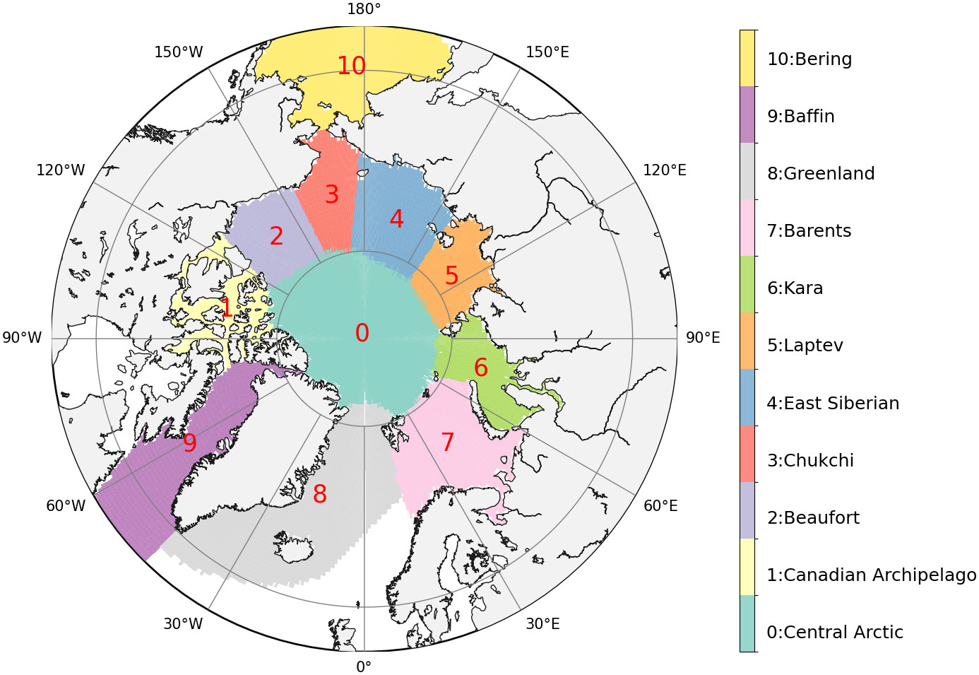
Figure 1 Subregions of the Arctic Ocean with the same definition in Li et al. (2021) and Kumar et al. (2021), which are shaded with 11 different colors.
2.3 Taylor diagram
Taylor diagrams provide a way to graphically summarize how well model simulations match observations (Taylor and Karl, 2001), and have been widely used in model evaluations (Mu et al., 2018; Kumar et al., 2021; Li et al., 2021). To compare the performance of different CMIP6 models on the same plot, here we have used the correlation coefficient (R), the normalized centered root mean square error (CRMSE), and the standard deviation (STD) in the Taylor diagrams, which are defined as follows:
Where and represent the SIT in the CMIP6 and PIOMAS models with a sample size of N, and their means are indicated by their overbars and , respectively.
3 Results
3.1 Mean state and seasonal cycle of SIT
Because of the lack of suitable satellite observations during the sea ice melt season, SIT observations are not continuous during the summer season. PIOMAS (version 2.1) provides an estimate of SIV from simulations with the assimilation of SIC and sea surface temperature observations (Zhang and Rothrock, 2003), which fill the SIT gaps in the summer. This product has been extensively validated against a wide range of observations, such as satellite and in situ mooring observations (Schweiger et al., 2011). Figure 2 shows the evolution of the monthly mean SIE and SIT in the Arctic Ocean from satellite observations, CMIP6 models, and the PIOMAS reanalysis. The biases of SIE between NSIDC observations, PIOMAS reanalysis, and MME of CMIP6 models are very small during the sea ice melt season (July-September) but the biases grow during the sea ice growth season (Figure 2A). The SIT of the PIOMAS reanalysis averaged for 2011-2022 agrees well with the CS2SMOS observations in winter, with biases of less than 0.3 m (Figure 2B). Although the CMIP6 models have a large ensemble spread, the MME from 1980 to 2014 shows good agreement with PIOMAS (Figure 2B). This gave us the confidence to use PIOMAS to evaluate the mean state and seasonal cycle of SIT from the selected 12 CMIP6 models based on the PIOMAS reanalysis.
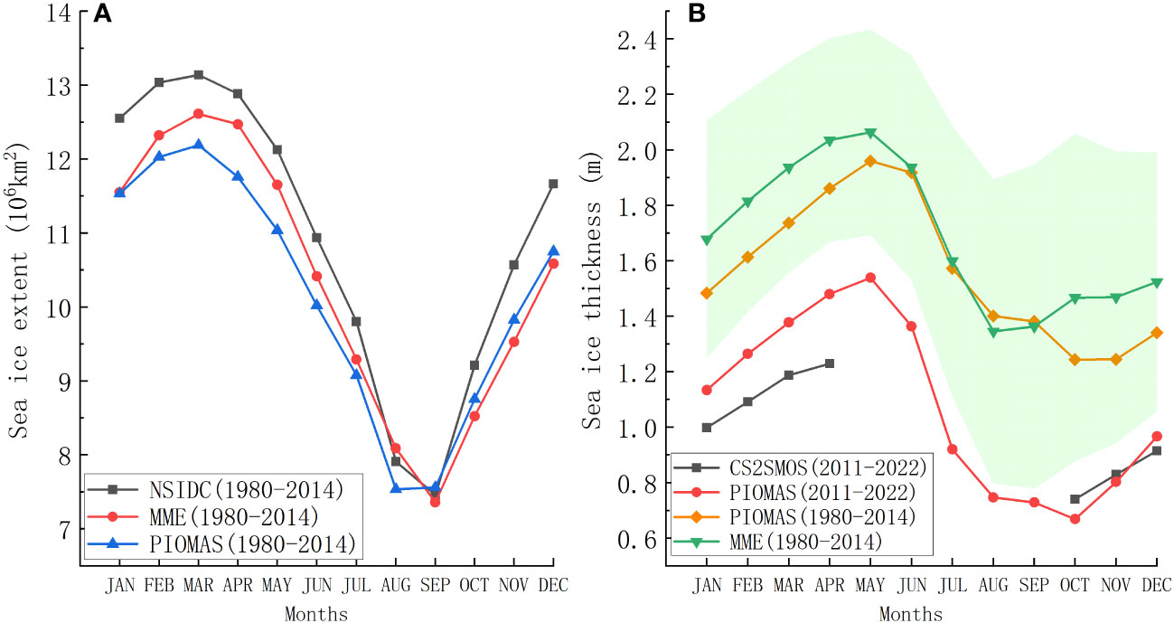
Figure 2 (A) Monthly climatological mean sea ice extent in the Arctic Ocean from NSIDC (black line), MME (red line), and PIOMAS reanalysis (blue line) from 1980 to 2014. (B) Monthly climatological mean sea ice thickness in the Arctic Ocean from PIOMAS reanalysis (red line), and CS2SMOS observations (black line) from 2011 to 2022. The orange and green lines indicate the sea ice thickness from PIOMAS and MME, averaged from 1980 to 2014. The green shading denotes the ensemble spread in the CMIP6 models.
To further investigate the performance of CMIP6 models in simulating different SIT categories, we show the seasonal evolution of SIE covered by different SIT from MME and PIOMAS (Figure 3), using the same SIT category boundaries from Hunke and Elizabeth (2014) and Kumar et al. (2021): 0-0.6 m, 0.6-1.4 m, 1.4-2.4 m, 2.4-3.6 m, and > 3.6 m. Overall, the SIE difference between MME and PIOMAS was very small, with biases of less than 1.0×10⁶ km2 throughout the year. The ice thickness category with a range of 1.4-2.4 m (purple bars) had the largest bias in the first three months of the year (Figure 3B). In both the MME and PIOMAS, we can also see that the fraction of sea ice coverage was dominated by ice with a thickness ranging from 1.4 m to 2.4 m in most months except April, May, and June, which were characterized by thicker ice, between 2.4 m and 3.6 m (Figure 3A). The percentage of ice thickness greater than 3.6 m was the smallest among the five SIT categories (Figure 3A), and the bias between MME and PIOMAS was also the smallest (Figure 3B) implying that the MME model represents the SIE of thick ice well. For thin ice of less than 0.6 m, we can see that the biases between MME and PIOMAS were also very small in all months (Figure 3B). This suggests that the MME can also represent the SIE of thin ice well.
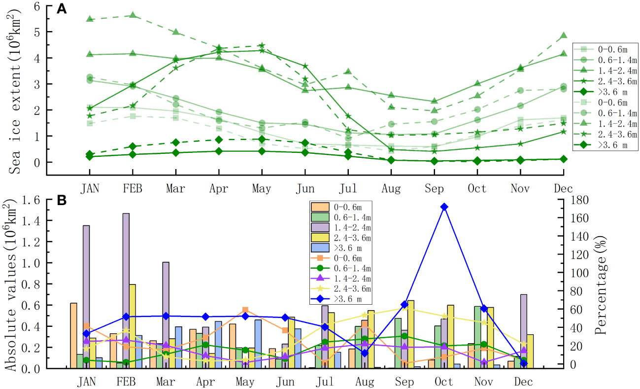
Figure 3 (A) Monthly mean SIE covered by different SIT categories from MME (solid line) and PIOMAS (dashed line) from 1980 to 2014. (B) Absolute values (bars) of SIE differences between MME and PIOMAS and the bias in percent of SIE differences relative to PIOMAS SIE.
3.2 Spatial distributions of SIT
To investigate the spatial distribution of SIT in March and September in the Arctic Ocean, we plotted the SIT averaged from 1980 to 2014 from the PIOMAS and CMIP6 models. As shown in Figures 4A, B, most regions of the Arctic Ocean are covered by sea ice during the winter. The ice-covered area in the MME is larger than that in the PIOMAS (purple lines), particularly in the Bering Sea, Baffin Sea, Greenland Sea, and Barents Sea, where the ocean is covered by thin new ice with SIT less than 0.5 m. This result is consistent with a previous study by Li et al. (2021). Compared to SIT in PIOMAS, the MME SIT is much larger in the Chukchi Sea, the Beaufort Sea, and the central Arctic, but smaller in the Greenland Sea (Figure 4C), with differences greater than 1 m in some regions. The thin new ice melts during the summer season (Figures 4D, E), so we can see the sea ice retreat in the Bering Sea, Chukchi Sea, Barents Sea, Greenland Sea, and Baffin Sea. As a result, most regions in the Arctic Ocean are covered by thick ice with a SIT greater than 0.5 m. The sea ice areas between PIOMAS and MME are very similar, but there is more sea ice in the Kara Sea in PIOMAS than in the MME. The SIT in the central Arctic is much larger in PIOMAS than in MME, but it is smaller in the other ice-covered regions (Figure 4F).
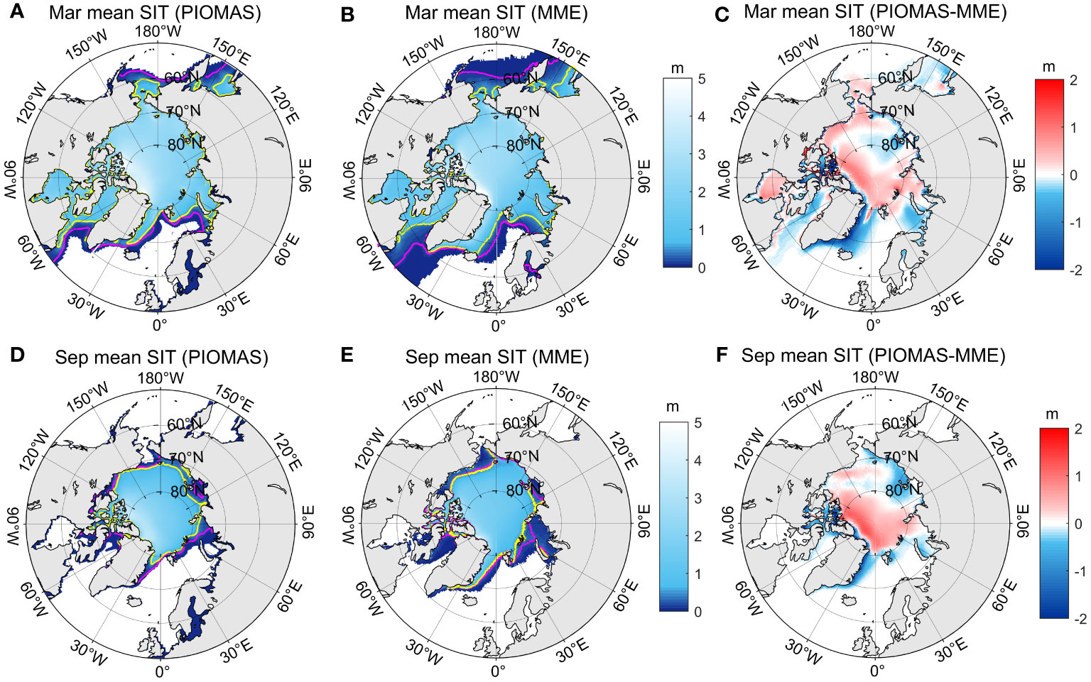
Figure 4 Spatial distributions of SIT averaged between 1980 and 2014 from (A) PIOMAS and (B) MME in March, and (C) the differences between PIOMAS and MME. The purple lines in (A) and (B) indicate the ice edge (SIC of 15%) from PIOMAS and MME, respectively, while the yellow lines indicate the ice thickness of 0.5 m. (D-F) Same as (A-C), but for September.
Due to the sea ice melting and refreezing in the Arctic Ocean, the interannual variability of SIT varies in different regions. To examine the difference in the interannual variability of SIT between PIOMAS and MME, we present the spatial distributions of the variance of the annual mean SIT (Figure 5). The variances of the annual mean SIT in PIOMAS are very small in most of the Arctic Ocean, except for the Canadian Archipelago and East Siberia (Figure 5A). The variances of the annual mean SIT in MME have a similar pattern to PIOMAS (Figure 5B), but with larger variances along the east coast of Greenland, implying that the SIT in CMIP6 models has larger interannual variability around this region. Additionally, we also show the variances of the mean SIT during the sea ice growth and melting seasons. Regions with strong interannual variability of SIT in March (Figures 5C, D) and September (Figures 5E, F) are similar to those in Figures 5A, B but with much larger amplitudes. The interannual variability of SIT in PIOMAS is stronger than that in the MME during these two seasons.
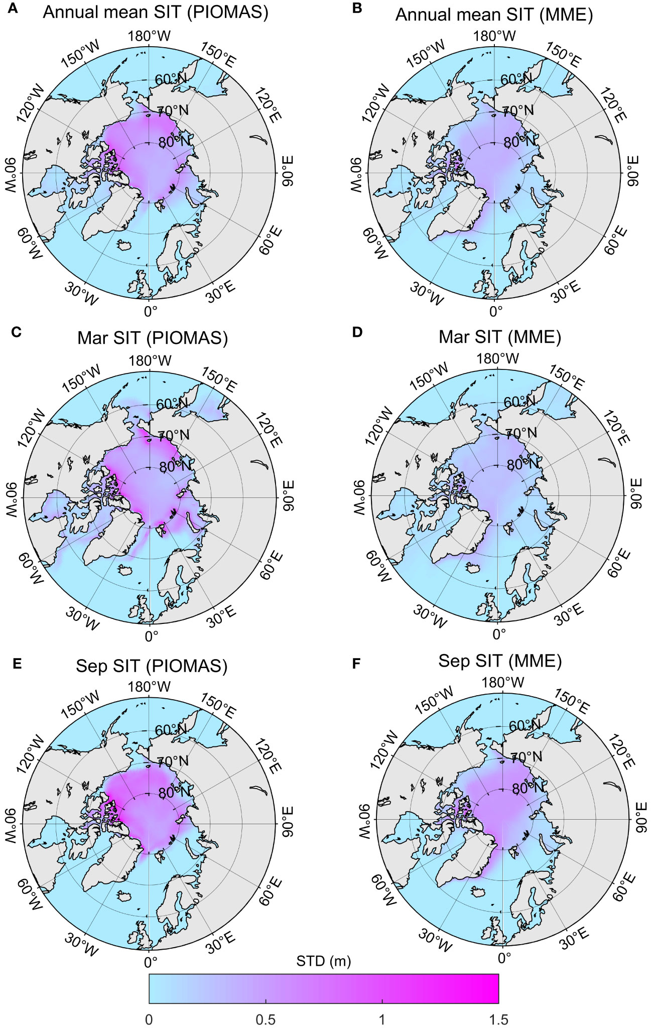
Figure 5 Spatial distributions of the variance of the annual mean SIT between 1980 and 2014 from (A) PIOMAS and (B) MME. (C, D) and (E, F) same as (A, B), but for March and September, respectively.
We further show the linear trends in SIT between 1980 and 2014 in the winter (Figures 6A, B) and summer (Figures 6C, D) seasons. We observe decreasing trends in SIT over the whole Arctic Ocean in all seasons, which is consistent with previous studies (Kwok et al., 2013; Tilling et al., 2019). Compared to the March SIT trends in PIOMAS (Figure 6A), we can also see negative trends along the eastern coast of Greenland and the Baffin Sea in the MME (Figure 6B). The areas with negative trends retreat in September, but the decreasing trends are much larger (Figures 6C, D), particularly in PIOMAS. As there is some thin sea ice from the MME along the eastern coast of Greenland in September (Figure 4E), we can still see negative trends of SIT in the MME (Figure 6D).
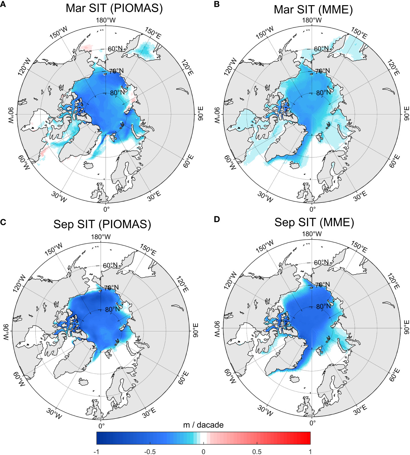
Figure 6 Spatial distributions of (A) PIOMAS and (B) MME SIT trends between 1980 and 2014 in March. (C, D) same as (A, B), but for September.
As shown in Figure 7, the climatological mean SIT in PIOMAS between 1980 and 2014 was 1.61 m, with an STD of 0.22 m. The largest SIT could be found in the SAM0-UNICON model, which reached 3.13 m. NESM3 had the smallest SIT, with a value of 1.03 m. This indicates that SAM0-UNICON and NESM 3 had the largest model biases in the climatological mean SIT over the Arctic Ocean compared to PIOMAS (blue bars). The same model biases could also be found in the mean SIT for March (orange bars) and September (gray bars). However, the model biases between PIOMAS and the 12 CMIP6 models were smaller in September than in March, suggesting that the CMIP6 models performed better in the sea ice melt season than in the sea ice growth season.
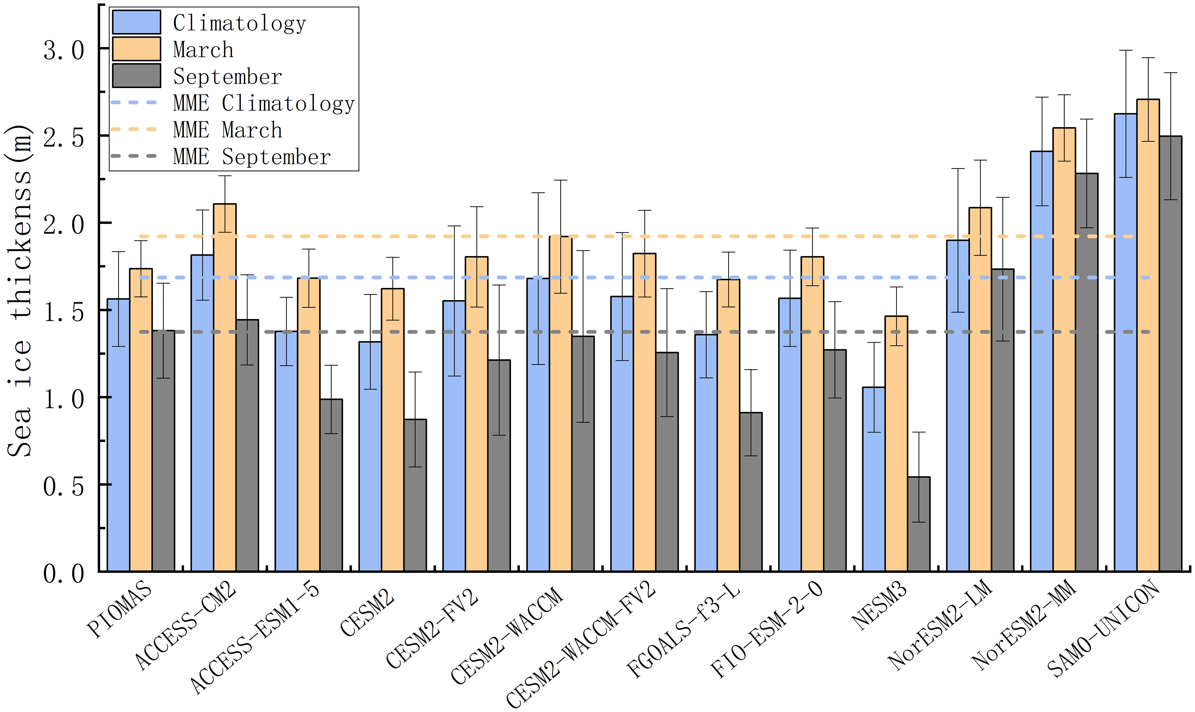
Figure 7 Sea ice thickness averaged between 1980 and 2014 from CMIP6 models and PIOMAS reanalysis. The blue, orange, and gray bars indicate the climatological mean SIT over the entire period, in March and September, respectively. The horizontal dashed lines denote the corresponding MME mean SIT. Error bars indicate significance at the 95% confidence level.
We then compared the monthly mean SIT between the PIOMAS and CMIP6 models. The monthly mean SIT of MME and PIOMAS peaked in May, and they decreased during the sea ice melt season, with a minimum MME SIT in August and a minimum PIOMAS SIT in October (Figure 8A). The monthly mean SIT differences between MME and PIOMAS were within 0.10 m, which occurred in summer (June-September). Compared to PIOMAS, the SAM0-UNICON model had the largest SIT difference, which was 1.41 m in October and 1.06 m for the entire 12 months. The SIT difference between the FIO-ESM-2.0 model and PIOMAS averaged over 12 months was only 0.004 m, suggesting that this model performed the best in seasonal cycles among the 12 CMIP6 models.
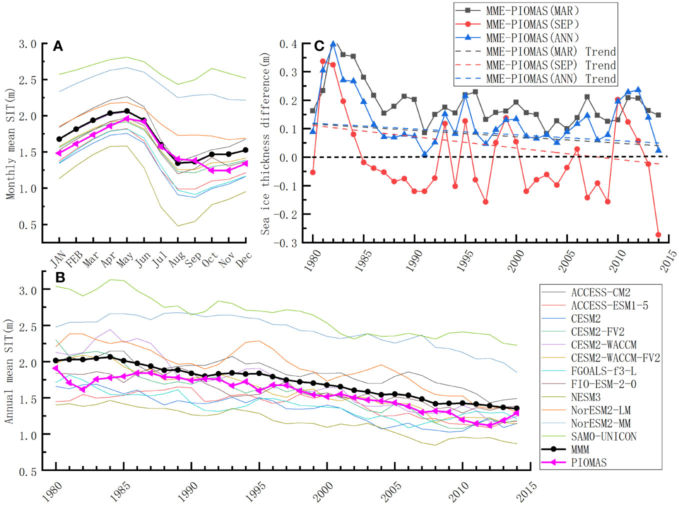
Figure 8 Monthly (A) and annual (B) climatological mean SIT in the Arctic Ocean between 1980 and 2014. (C) Monthly evolution of the difference between MME and PIOMAS from 1980 to 2014 in March (black line), September (red line), and the annual mean (blue line). The dashed lines indicate the corresponding linear trends.
At interannual time scales, we found decreasing SIT trends and interannual variability in PIOMAS and all CMIP6 models from 1980 to 2014 (Figure 8B), consistent with previous studies (Cavalieri and Parkinson, 2012; Bindoff et al., 2019). The annual mean MME showed consistent variability with PIOMAS, with differences of less than 0.28 m. Among the 12 CMIP6 models, the SAM0-UNICON had the largest positive bias compared to PIOMAS, with a value of 1.28 m in 1985, and the NESM 3 model had the largest negative bias, -0.65 m, in 1997. Overall, the FIO-ESM-2.0 model had the smallest difference of 0.11 m over the whole period between 1980 and 2014, which was the best simulation of the annual mean SIT. The differences between MME and PIOMAS in March and September and the annual mean from 1980 to 2014 were within 0.4 m (Figure 8C). The smallest differences occurred between 1990 and 2010, which were less than 0.15 m. We could also find decreasing trends in the differences between MME and PIOMAS, which indicates that the performance of CMIP6 models has improved over the past decades.
Figure 9 shows the simulation skills of the CMIP6 models. We found that most models have correlation coefficients of 0.8-0.9 and CRMSEs of 0.3-0.9 m. The correlation coefficients in almost all CMIP6 models were larger than 0.8, except the SAM0-UNICON model, which had a correlation coefficient of 0.7. The MME showed the highest correlation with PIOMAS, with a correlation coefficient of 0.93 (above the 95% significance level). Additionally, the CRMSE of the MME was the smallest among all CMIP6 models, with a value of 0.37. The SAM0-UNICON and CESM2-WACCM had CRMSE greater than 0.75, implying large biases in these two models. It was also shown that the NorESM2-MM model had the smallest variability, but the SIT variability in CESM2-WACCM was the highest. These results further demonstrate that the SAM0-UNICON model performs worse than the other CMIP6 models shown in Figures 7, 8, suggesting that it is necessary to use the MME results to better represent the sea ice evolution in the CMIP6 models.
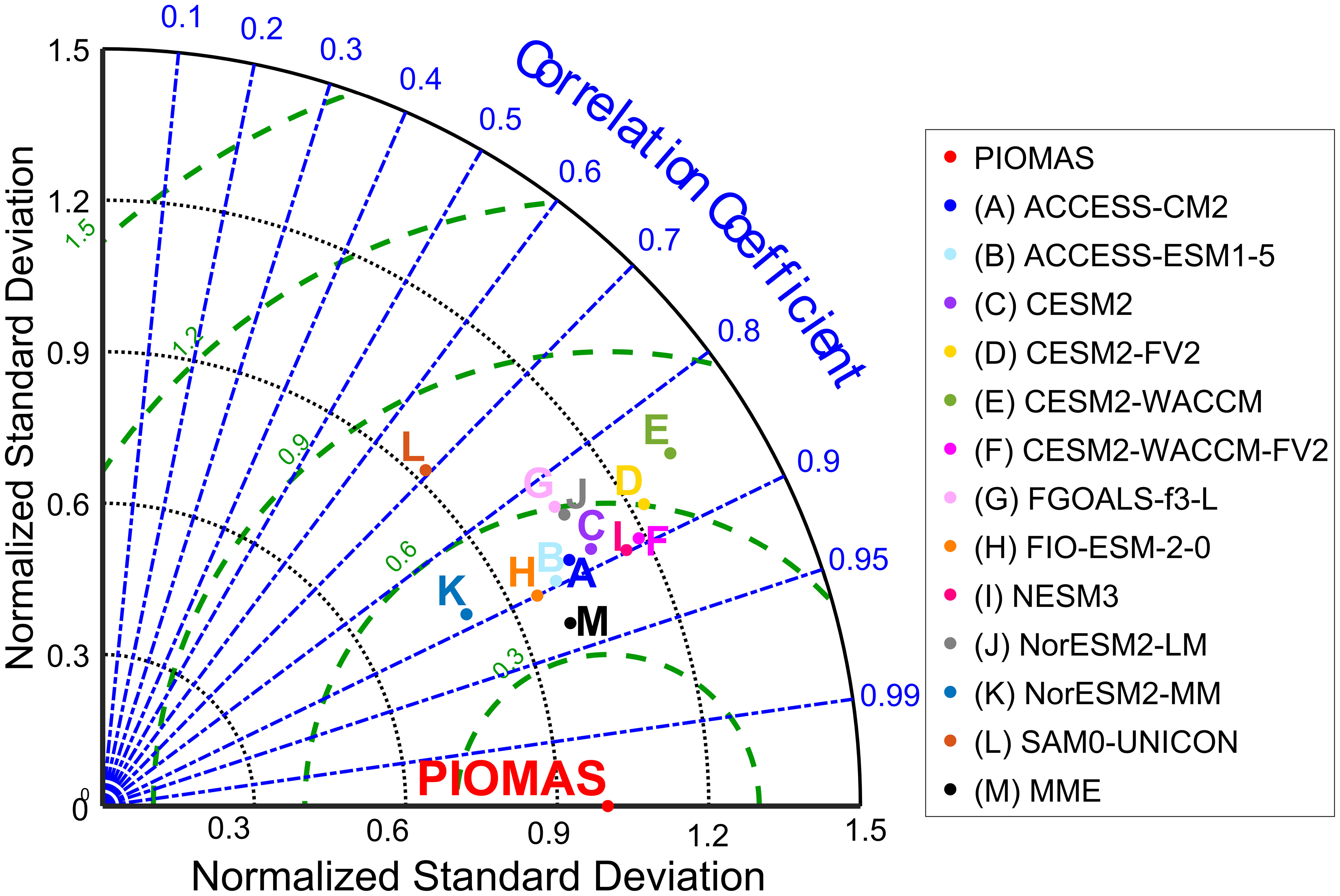
Figure 9 Taylor diagrams displaying statistical comparisons of monthly mean SIT over the Arctic Ocean from January 1980 to December 2014 between different models and PIOMAS. The blue, green, and gray lines represent the correlation coefficient, normalized centered root mean square errors, and standard deviations, respectively. PIOMAS is indicated with the red dot.
4 Discussion and conclusion
In this study, we evaluated the SIT simulation in 12 CMIP6 models using satellite observations and PIOMAS reanalysis. We assessed not only the mean state, seasonal cycle, and spatial distributions of SIT but also the intercomparison of SIT simulations in 12 CMIP6 models. We found that the CMIP6 MME can well represent the mean state and monthly cycle of SIT in the Arctic Ocean. The variances of the annual mean SIT in PIOMAS are very small in most of the Arctic Ocean. We also found decreasing trends in SIT over the entire Arctic Ocean in all seasons. The CMIP6 models performed better in the sea ice melt season than in the sea ice growth season. The FIO-ESM-2.0 model performed the best among 12 CMIP6 models in seasonal cycles, but the SAM0-UNICON model had the largest bias and performed worse than the other CMIP6 models.
We chose 12 CMIP6 models with CICE components and compared their performance in simulating the SIT in the Arctic Ocean. Our results showed that the model performances vary in different CMIP6 models, although with the same sea ice component. Various factors can cause the SIT biases in CMIP6 models. On the one hand, the bias can originate from the CICE model, e.g., the version of the CICE model, the uncertainty of the subgrid-scale ice thickness distributions and ice thickness categorization, etc. (Urrego-Blanco et al., 2016; Wang et al., 2020). On the other hand, the CICE model is coupled with ocean and atmosphere models that transfer heat, salt, and momentum fluxes to the ice model (Kumar et al., 2021; Yu et al., 2022). Biases from unrealistically simulated surface air and ocean temperature, 10 m winds, snowfall/depth, and surface albedo or coarse spatial resolution can also affect the SIT simulation in the CICE model (Crawford et al., 2023). Our study shows which combination of CICE, ocean, and atmosphere models in CMIP6 is the best, which will be beneficial for the development of the next generation of CMIP models with a CICE component.
In addition to the CICE components, there are also other sea ice model components in CMIP6, such as FESOM, SIS2, LIM3, GFDL, GISS SI, NEMO-LIM3, COCO 4.9, and MPIOM 1.63. Although previous studies have evaluated the SIT simulations in FESOM, LIM3, and NEMO-LIM3 (Pemberton et al., 2017; Semmler et al., 2020; Tian et al., 2021), our understanding of the SIT simulations in the other sea ice models is limited. Therefore, further investigations are needed to assess the SIT simulations in the CMIP6 models with the other sea ice model components.
As shown in Figures 4–6, the biases, variability, and trends of SIT vary in different subregions. Previous studies have shown different changes in SIT and SIE in the Arctic Ocean. For example, the edge of the seasonal Arctic sea ice is constantly retreating toward the central Arctic under global warming, resulting in a decrease in SIE (Meier et al., 2007). SIT also decreased by 36% in the western and central Arctic from the 1980s to the early 2000s (Kwok and Rothrock, 2009). The decrease in SIT will further reduce sea ice cover and increase the area of the open ocean (Park et al., 2015). The decreasing rate of SIE is the largest in the Beaufort and Chukchi Seas, with values of 0.36×10⁵ km2/year (Hu et al., 2022). Our results show that the decreasing trends of SIT vary in different subregions of the Arctic Ocean. However, our understanding of SIT simulations in CMIP6 models with CICE components in these subregions is limited and needs further evaluation.
Data availability statement
The CS2SMOS product version v205 can be downloaded from https://data.seaiceportal.de/data/cs2smos_awi/. The PIOMAS reanalysis (version 2.1) is available at http://psc.apl.uw.edu/research/projects/arctic-sea-ice-volume-anomaly/. The CMIP6 model simulations can be accessed from https://esgf-node.llnl.gov/projects/cmip6/. The NOAA/NSIDC Climate Data Record of Passive Microwave Sea Ice Concentration, Version 3 datasets, are obtainable from https://nsidc.org/data/G02202/versions/3.
Author contributions
JL conceived the study and developed the conceptual framework. MX analyzed the results and plotted the figures. All authors contributed to the interpretation of the results and the writing and editing of the manuscript. All authors contributed to the article and approved the submitted version.
Funding
This study was funded by the National Science Foundation Funds of China (41706008, 42130409), the Fundamental Research Funds for the Central Universities, China (1074-423102), Hohai University (522020512), and the Jiangsu Provincial Innovation and Entrepreneurship Program (JSSCRC2021492).
Conflict of interest
The authors declare that the research was conducted in the absence of any commercial or financial relationships that could be construed as a potential conflict of interest.
Publisher’s note
All claims expressed in this article are solely those of the authors and do not necessarily represent those of their affiliated organizations, or those of the publisher, the editors and the reviewers. Any product that may be evaluated in this article, or claim that may be made by its manufacturer, is not guaranteed or endorsed by the publisher.
References
AWI (2023). ESA cryoSat-2/SMOS merged product description document (PDD) (Paris, France: ESA-European Space Agency). Available at: https://data.seaiceportal.de/data/cs2smos_awi/.
Balan-Sarojini B., Tietsche S., Mayer M., Balmaseda M., Zuo H. (2021). Year-round impact of winter sea ice thickness observations on seasonal forecasts. Cryosphere 15 (1), 325–344. doi: 10.5194/tc-2020-73
Bindoff N. L., Cheung W., Kairo J. G., Aristegui J., Whalen C. (2019). Changing ocean, marine ecosystems, and dependent communities. IPCC Special Rep. Ocean Cryosphere Changing Climate 477–587. doi: 10.1017/9781009157964.007
Cai D., Lohmann G., Chen X., Ionita M. (2023). The linkage between autumn Barents-Kara sea ice and European cold winter extremes. EGUsphere, 1–26. doi: 10.5194/egusphere-2023-1646
Cavalieri D. J., Parkinson C. L. (2012). Arctic sea ice variability and trend-2010. Cryosphere 6 (4), 881–889. doi: 10.5194/tc-6-881-2012
Chatterjee S., Ravichandran M., Murukesh N., Raj R. P., Johannessen O. M. (2021). A possible relation between Arctic sea ice and late season Indian Summer Monsoon Rainfall extremes. Climate Atmospheric Sci. 4, 36. doi: 10.1038/s41612-021-00191-w
Collow T. W., Wang W., Kumar A., Zhang J. (2015). Improving arctic sea ice prediction using PIOMAS initial sea ice thickness in a coupled ocean–atmosphere model. Mon. Weather Rev. 143 (11), 4618–4630. doi: 10.1175/mwr-d-15-0097.1
Comiso J. C., Meier W. N., Gersten R. (2017). Variability and trends in the Arctic Sea ice cover: Results from different techniques. J. Geophys. Res.: Oceans 122 (8), 6883–6900. doi: 10.1002/2017JC012768
Crawford A. D., Rosenblum E., Lukovich J. V., Stroeve J. C. (2023). Sources of seasonal sea-ice bias for CMIP6 models in the Hudson Bay Complex. Ann. Glaciology, 1–18. doi: 10.1017/aog.2023.42
Döscher R., Vihma T., Maksimovich E. (2014). Recent advances in understanding the Arctic climate system state and change from a sea ice perspective: a review. Atmos. Chem. Phys. 14 (24), 13571–13600. doi: 10.5194/acp-14-13571-2014
Feldl N., Merlis T. M. (2021). Polar amplification in idealized climates: the role of ice, moisture, and seasons. Geophysical Res. Lett. 48, e2021GL094130. doi: 10.1029/2021gl094130
Francis J. A., Wu B. (2020). Why has no new record-minimum Arctic sea-ice extent occurred since September 2012? Environ. Res. Lett. 15 (11), 114034. doi: 10.1088/1748-9326/abc047
Frey K. E., Perovich D. K., Light B. (2011). The spatial distribution of solar radiation under a melting Arctic sea ice cover. Geophys. Res. Lett. 38 (22), L22501. doi: 10.1029/2011gl049421
Hu H., Zhang Z., Li X. (2022). Spatiotemporal variations of Arctic multi-year ice from 2000 to 2019. Chin. J. of Polar Res. 34 (4), 419–430. doi: 10.13679/j.jdyj.20210070
Hunke, Elizabeth C. (2014). Sea ice volume and age: Sensitivity to physical parameterizations and thickness resolution in the CICE sea ice model. Ocean Model. 82, 45–59. doi: 10.1016/j.ocemod.2014.08.001
Johnson M., Proshutinsky A., Aksenov Y., Nguyen A. T., Lindsay R. (2012). Evaluation of Arctic sea ice thickness simulated by Arctic Ocean Model Intercomparison Project models. J. Geophys. Res. Oceans 117, C00D13. doi: 10.1029/2011JC007257
Kacimi S., Kwok R. (2022). Arctic snow depth, ice thickness, and volume from ICESat-2 and cryoSat-2: 2018–2021. Geophysical Res. Lett. 49, e2021GL097448. doi: 10.1029/2021gl097448
Koenigk T., Devasthale A., Karlsson K. G. (2014). Summer Arctic sea ice albedo in CMIP5 models. Atmos. Chem. Phys. 14 (4), 1987–1998. doi: 10.5194/acp-14-1987-2014
Kumar R., Li J., Hedstrom K., Babanin A. V., Tang Y. (2021). Intercomparison of Arctic sea ice simulation in ROMS-CICE and ROMS-Budgell. Polar Sci. 29, 100716. doi: 10.1016/j.polar.2021.100716
Kwok R. (2018). Arctic sea ice thickness, volume, and multiyear ice coverage: losses and coupled variability, (1958–2018). Environ. Res. Lett. 13, 105005. doi: 10.1088/1748-9326/aae3ec
Kwok R., Rothrock D. A. (2009). Decline in Arctic sea ice thickness from submarine and ICESat records: 1958-2008. Geophys. Res. Lett. 36 (15), L15501. doi: 10.1029/2009gl039035
Kwok R., Spreen G., Pang S. (2013). Arctic sea ice circulation and drift speed: Decadal trends and ocean currents. J. Geophys. Res.: Oceans 118 (5), 2408–2425. doi: 10.1002/jgrc.20191
Lang A., Yang S., Kaas E. (2016). Sea ice thickness and recent Arctic warming. Geophys. Res. Lett. 44 (1), 409–418. doi: 10.1002/2016GL071274
Li J., Babanin A. V., Liu Q., Voermans J. J., Heil P., Tang Y. (2021). Effects of wave-induced sea ice break-up and mixing in a high-resolution coupled ice-ocean model. J. Mar. Sci. Eng. 9, 365. doi: 10.3390/JMSE9040365
Mallett R. D. C., Stroeve J. C., Tsamados M., Landy J. C., Willatt R., Nandan V., et al. (2020). Faster decline and higher variability in the sea ice thickness of the marginal Arctic seas when accounting for dynamic snow cover. The Cryosphere 15, 2429–2450. doi: 10.5194/tc-15-2429-2021
Meier W. N., Fetterer F., Savoie M., Mallory S., Duerr R., Stroeve. J. (2017). NOAA/NSIDC climate data record of passive microwave sea ice concentration; version 3 (Boulder, CO, USA: NSIDC—National Snow and Ice Data Center). Available at: http://nsidc.org/data/seaice_index/.
Meier W. N., Stroeve J., Fetterer F. (2007). Whither Arctic sea ice_ A clear signal of decline regionally, seasonally and extending beyond the satellite record. Ann. Glaciol. 46, 428–434. doi: 10.3189/172756407782871170
Mu L., Losch M., Yang Q., Ricker R., Loza S. N., Nerger L. (2018). Arctic-wide sea ice thickness estimates from combining satellite remote sensing data and a dynamic ice-ocean model with data assimilation during the CryoSat-2 period. J. Geophys. Res.: Oceans 123, 7763–7780. doi: 10.1029/2018jc014316
Notz D., Community S. (2020). Arctic sea ice in CMIP6. Geophys. Res. Lett. 47, e2019GL086749. doi: 10.1029/2019GL086749
Park H.-S., Lee S., Son S.-W., Feldstein S. B., Kosaka Y. (2015). The impact of poleward moisture and sensible heat flux on arctic winter sea ice variability*. J. Climate 28 (13), 5030–5040. doi: 10.1175/jcli-d-15-0074.1
Pemberton P., Löptien U., Hordoir R. (2017). Sea-ice evaluation of NEMO-Nordic 1.0: a NEMO–LIM3.6-based ocean–sea-ice model setup for the North Sea and Baltic Sea. Geosci. Model. Dev. 10 (8), 3105–3123. doi: 10.5194/gmd-10-3105-2017
Previdi M., Janoski T. P., Chiodo G. (2020). Arctic amplification: A rapid response to radiative forcing. Geophys Res. Lett. 47, e2020GL089933. doi: 10.1029/2020gl089933
Ricker R., Hendricks S., Kaleschke L., Tian-Kunze X., King J., Haas C. (2017). A weekly Arctic sea-ice thickness data record from merged CryoSat-2 and SMOS satellite data. Cryosphere 11 (4), 1607–1623. doi: 10.5194/tc-11-1607-2017
Schweiger A., Lindsay R., Zhang j., Steele M., Stern H. (2011). Uncertainty in modeled Arctic sea ice volume. J. Geophys. Res.: Oceans 116 (C8), C00D06. doi: 10.1029/2011JC007084
Screen J. A., Deser C., Simmonds I. (2012). Local and remote controls on observed Arctic warming. Geophys. Res. Lett. 39 (10), 10709. doi: 10.1029/2012GL051598
Semmler T., Danilov S., Gierz P. (2020). Simulations for CMIP6 with the AWI climate model AWI-CM-1-1. J. Adv. Model. Earth Sy. 12, e2019MS002009. doi: 10.1029/2019ms002009
Serreze M. C., Barry R. G. (2011). Processes and impacts of Arctic amplification: A research synthesis. Global planetary Change 77 (1-2), 85–96. doi: 10.1016/j.gloplacha.2011.03.004
Shu Q., Song Z., Qiao F. (2015). Assessment of sea ice simulations in the CMIP5 models. Cryosphere 9 (1), 399–409. doi: 10.5194/tc-9-399-2015
Stjern C. W., Lund M. T., Samset B. H. (2019). Arctic amplification response to individual climate drivers. J. Geophys. Res. Atmos 124 (13), 6698–6717. doi: 10.1029/2018jd029726
Stroeve J. C., Serreze M. C., Holland M. M., Kay J. E., Malanik J., Barrett A. P. (2012). The Arctic's rapidly shrinking sea ice cover: a research synthesis. Clim. Change 110 (3-4), 1005–1027. doi: 10.1007/s10584-011-0101-1
Taylor, Karl E. (2001). Summarizing multiple aspects of model performance in a single diagram. J. Geophys. Res. Atmos 106 (D7), 7183–7192. doi: 10.1029/2000JD900719
Tian T., Yang S., Karami M. P., Massonnet F., Kruschke T., Koenigk T. (2021). Benefits of sea ice initialization for the interannual-to-decadal climate prediction skill in the Arctic in EC-Earth3. Geosci. Model. Dev. 14 (7), 4283–4305. doi: 10.5194/gmd-14-4283-2021
Tilling R., Ridout A., shepherd A. (2019). Assessing the impact of lead and floe sampling on arctic sea ice thickness estimates from envisat and cryoSat-2. J. Geophys. Res. Oceans 124 (11), 7473–7485. doi: 10.1029/2019JC015232
Tsujino H., Urakawa L. S., Griffies S. M., Danabasoglu G., Yu Z. (2020). Evaluation of global ocean–sea-ice model simulations based on the experimental protocols of the Ocean Model Intercomparison Project phase 2 (OMIP-2). Geosci. Model. Dev. 13 (8), 3643–3708. doi: 10.5194/gmd-2019-363
Uotila P., Goosse H., Haines K., Chevallier M., Barthélemy A., Bricaud C., et al. (2019). An assessment of ten ocean reanalyses in the polar regions. Clim. Dyn 52 (3), 1613–1650. doi: 10.1007/S00382-018-4242-Z
Urrego-Blanco J. R., Urban N. M., Hunke E. C., Turner A. K., Jeffery N. (2016). Uncertainty quantification and global sensitivity analysis of the Los Alamos sea ice model. J. Geophysical Research: Oceans 121 (4), 2709–2732. doi: 10.1002/2015jc011558
Wang H., Zhang L., Chu M., Hu S. (2020). Advantages of the latest Los Alamos Sea-Ice Model (CICE): evaluation of the simulated spatiotemporal variation of Arctic sea ice. Atmospheric Oceanic Sci. Lett. 13 (2), 113–120. doi: 10.1080/16742834.2020.1712186
Wang X. J., Key J., Zhang J. (2016). Comparison of arctic sea ice thickness from satellites, aircraft, and PIOMAS data. Remote Sens. 8 (9), 713. doi: 10.3390/rs8090713
Yu L., Liu J., Gao Y., Shu Q. (2022). A sensitivity study of arctic ice-ocean heat exchange to the three-equation boundary condition parametrization in CICE6. Adv. Atmospheric Sci. 39 (9), 1398–1416. doi: 10.1007/s00376-022-1316-y
Zachary G., Magnusdottir, Stern H. (2018). Variability of arctic sea ice thickness using PIOMAS and the CESM large ensemble. J. Clim. 31 (8), 3233–3247. doi: 10.1175/jcli-d-17-0436.1
Zhang Y., Chao N., Li F., Yue L., Wang S., Chen G., et al. (2023). Reconstructing long-term arctic sea ice freeboard, thickness, and volume changes from envisat, cryosat-2, and ICESat-2. J. Mar. Sci. Eng. 11, 979. doi: 10.3390/jmse11050979
Zhang J., Rothrock D. A. (2003). Modeling global sea ice with a thickness and enthalpy distribution model in generalized curvilinear coordinates. Mon. Weather Rev. 131 (5), 845–861. doi: 10.1175/1520-0493(2003)131<0845:MGSIWA>2.0.CO;2
Keywords: sea ice thickness, PIOMAS, CICE MME, CMIP6, Arctic Ocean
Citation: Xu M and Li J (2023) Assessment of sea ice thickness simulations in the CMIP6 models with CICE components. Front. Mar. Sci. 10:1223772. doi: 10.3389/fmars.2023.1223772
Received: 16 May 2023; Accepted: 27 September 2023;
Published: 18 October 2023.
Edited by:
Junhong Liang, Louisiana State University, United StatesReviewed by:
Haijin Dai, National University of Defense Technology, ChinaValentin Ludwig, Alfred Wegener Institute Helmholtz Centre for Polar and Marine Research (AWI), Germany
Copyright © 2023 Xu and Li. This is an open-access article distributed under the terms of the Creative Commons Attribution License (CC BY). The use, distribution or reproduction in other forums is permitted, provided the original author(s) and the copyright owner(s) are credited and that the original publication in this journal is cited, in accordance with accepted academic practice. No use, distribution or reproduction is permitted which does not comply with these terms.
*Correspondence: Junde Li, anVuZGUubGlAaGh1LmVkdS5jbg==