 Bijan Dargahi
95% of researchers rate our articles as excellent or good
Learn more about the work of our research integrity team to safeguard the quality of each article we publish.
Find out more
ORIGINAL RESEARCH article
Front. Mar. Sci. , 03 November 2023
Sec. Deep-Sea Environments and Ecology
Volume 10 - 2023 | https://doi.org/10.3389/fmars.2023.1223654
This article is part of the Research Topic Environmental Impacts & Risks of Deep-Sea Mining: Recommendations for Exploitation Regulations View all 10 articles
The discovery of rare metal resources in international waters has raised seabed mining claims for large areas of the bottom. There is abundant scientific evidence of major negative consequences for the maritime environment, such as the destruction of natural landforms and the fauna that depend on them, as well as the production of enormous silt plumes that disrupt aquatic life. This study investigated the environmental risks of seabed mining for metal resources in the Baltic Sea using a combination of hydrodynamic, particle-tracking, and sediment-transport models. The models were applied for ten years i.e., 2000-2009 under prevailing conditions to simulate seabed mining operations. The focus was on sediment concentration near the seabed and its spread. The mean background concentrations were low with small seasonal bed-level variations throughout the Baltic Sea Basin. Late summer and early autumn periods were the most active. Seabed mining significantly alters the dynamics of sediment suspensions and bed level variations. The concentrations increase unsustainably to high levels, posing a serious threat to the ecological health of the Baltic Sea. The Gotland basins in the Baltic Sea are the most susceptible to mining. The bed level variations will be ten-fold, exposing the highly contaminated sediments at the seabed to the flow. In less than a year, 30-60% of the total particles released in each basin reached the thermocline layers. This study suggests that seabed mining in the Baltic Sea is not sustainable.
Seabed mining affects the dynamics of suspended sediment loads near the seabed and in the water column, which is correlated with various environmental problems It is encouraging to see a growing public awareness of seabed mining as a possible serious environmental threat to the oceans. In this case, the scientific community plays an important role in analyzing and scrutinizing various aspects of seabed mining. To quote Earle and Kammen (2022) on seabed mining “Seldom do we have an opportunity to stop an environmental crisis before it begins. This is one of those opportunities”.
The introduction describes numerous aspects of energy needs, mining technology, and environmental implications of seabed mining, with a focus on sediment plume development, modelling methodologies, and the current state of the Baltic Sea, which is the main area investigated in this study. The goal was to present a brief overview of ongoing efforts on various elements of seabed mining.
There is an exponentially growing worldwide demand for electric transportation to reduce negative trends in global climate change. The details of worldwide energy consumption in different sectors are available from U.S. Energy Information Administration (2016) and Enerdata (2022). Published data indicate 23,845 TWh of energy were used in 2019. Generally, transportation accounts for 25% and industries, including residential housing and commercial businesses, account for 35% of the total energy. Considering the focus of seabed mining on transportation, the present battery demand is 340 GWh, which will grow to 3500 GWh, which is far beyond the total available land resources IEA (2022). The discovery of the majority of rare metal resources in international waters (mostly in the Pacific Ocean) has increased the claims of seabed mining contractors to significant regions of the seafloor (Sharma, 2015). The International Seabed Authority granted 31 contracts to investigate deep-sea mineral resources as of May 2022. The global seabed designated for resource exploration has a size of 1.45 million km2, which is roughly equal to the surface areas of France, Germany, and Spain (IUCN, 2022).
Mining technology is undergoing further technical developments. Examples of possible technical details and operational modes of deep-sea mining have been discussed by researchers, including Hengling and Shaojun (2020). Mining machinery typically consists of four main units: a water pump, suction pipe, pressure pipe, and collector (Alhaddad et al., 2022). Mining operations on the seafloor create sediment plumes and turbidity currents. The excavated materials are pumped to a ship and wastewater and debris are dumped back into the ocean to form sediment clouds. The focus of the present study was on sediment plumes.
Most studies have used numerical modelling to investigate the dynamic characteristics of seabed mining (e.g. Jankowski and Zielke, 2001; Byishimo, 2018). Jankowski and Zielke (2001) developed a complicated mesoscale 3D numerical hydrodynamic and sediment transport model to investigate the impact of deep-sea activity on sediment concentration. The model also accounted for the influence of flocculation on sediment settling velocity. The overall bottom deposition patterns were successfully modelled, in agreement with the measurements. However, no conclusion could be drawn on the prognostic capability of the model because of the lack of complete datasets. Byishimo (2018) presented comprehensive Computational Fluid Dynamics (CFD) and laboratory studies on deep-sea mining, covering different aspects of plumes released at different water depths. It was found that particle settlement in the plume released near the bed was limited by the ambient currents that were carried far from the released currents in the same direction as the local ambient currents. The foregoing and similar studies show the strengths and weaknesses of numerical models for studying the impact of seabed mining on sediment transport. Numerical models can provide detailed results that are difficult to achieve using point measurements at preselected sites. However, they require field data for validation, which is currently scarce. Based on the success of these and similar models, a numerical approach was used to investigate the impact of SWM in the Baltic Sea.
A key difficulty in studying the impact of seabed mining is a lack of complete and consistent field data. Data are required to validate numerical models and to realistically represent the overall impact of mining machinery. This void can be filled in part by experimental and full-scale machinery tests. There have been several experimental and on-site studies. Muñoz-Royo et al. (2022) conducted an extensive field study on seabed mining in which the dynamics and spreading of sediment plumes created by collector vehicles were investigated in the Clarion Clipperton Zone in the Pacific Ocean at a depth of 4500 m. In a recent study, Peacock and Ouillon (2023) provided a comprehensive summary of the fluid mechanics in deep-sea mining. In situ, deep-sea plume experiments conducted on the Tropic Seamount by Spearman et al. (2020) showed that the suspended sediment concentration increased by 2.5 over the background concentration at 1.5 m above the bed. Muñoz-Royo et al. (2022) reported a value of 200 g/m3 within a 2-meter layer above the seabed in the Pacific Ocean for a deep-sea mining track of 100 m. The extent of the area “affected” was 100 m from the collector vehicle. However, the foregoing findings should not be considered universal as they are subject to many limitations and uncertainties. One is the lack of data on the long-term temporal and spatial variations of sediment plumes that are driven by the complicated hydrodynamic characteristics of the deep sea. These studies were also conducted at a few specific sites that might not be representative of the water body.
There is overwhelming scientific evidence of serious adverse effects on the sea environment. These include the destruction of natural landforms and the wildlife they support and the formation of large sediment plumes that disrupt aquatic life (for example, Ahnert and Borowski, 2000; DFO, 2000; Halfar and Fujita, 2007; Sharma, 2011; Van Dover et al., 2017; Miller et al., 2018; Orcutt et al., 2020; Scales, 2021; Farran, 2022).
The ocean receives each year extremely large quantities of trash and other pollutants through human activities from both point and nonpoint sources (NOAA, 2020). In recent decades, anthropogenic inputs of contaminants such as heavy metals into the marine environment have significantly increased (Ansari et al., 2004). These harmful substances settle and are deposited on the seabed sediments. The release of polluted suspended sediments through mining operations causes further contamination of seawater, posing a serious threat to ecosystems and marine habitats. The related changes in the water quality that support these habitats are mostly irreversible.
The habitats of benthic animals are also disturbed by the removal of portions of the seafloor depending on the type and location of mining and the formation of plumes. Sediment plumes can be detrimental to seabed ecology when mining operation creates clouds of floating particles. There are potentially two types of plumes: the plume created by the collector near the seabed and the plume created by discharge from the mining operation. In the latter case, near-bottom and mid-water plumes are formed, depending on where the discharge water from the mining platform would be released. Another important aspect is the amount of sediment removed during the mining operations. Sharma (2011) provided a sample calculation of the rate and extent of deep-sea mining. It is stated that nodule mining occurs at a rate of 3 million tons per year and a penetration depth of 10 cm, and the actual area scraped will be 600 km2/year (2 km2/day). However, according to Weaver et al. (2022), a more realistic removal rate is 200 km2.
In recent years, the Baltic Sea has received considerable attention owing to the possibility of implementing seabed mining projects for polymetallic nodules in several basins. This presents an alarming prospect regarding the vulnerability of its ecosystem. The ecological and marine health of the Baltic Sea is declining rapidly (Shahabi-Ghahfarokhi, 2022). The major problems are eutrophication, the accumulation of heavy metals, and various toxic chemicals in seabed sediments. One consequence is the hypoxia of the deeper waters in the Baltic Sea, mainly in the southern basins (Dargahi, 2022). It has been reported that the oxygen content in the deeper waters of the Baltic Sea has declined to unseen levels over the last 1500 years.
Annually, large amounts of hazardous substances and heavy metals (for example Cd, Hg, and Pb) enter the Baltic Sea through various rivers from neighboring countries (HELCOM, 2021). For example, the Baltic Sea receives 14.6 GBq 210Po annually from the Vistula River, with a mean discharge of 1080 m3/s (Skwarzec and Jahnz, 2007). More information is available from the Baltic Marine Environmental Protection Commission which maintains large databases on the marine environment, and different theme databases.
The available literature data suggest that the Baltic Sea seabed contains polymetallic nodules of iron and manganese that are found in the southern Baltic, around the Gulf of Bothnia, and the Gulf of Finland (Rolf, 1979; Kaikkonen et al., 2019). Currently, there is no accessible information regarding the type and nature of seabed mining in the Baltic Sea. However, recently, a Swedish company has been granted the exploration of mineral deposits in the Baltic Sea in the Bay of Bothnia. They are expecting 6-9 million polymetallic nodules (for example, Fe, Mg, Si, P, and Co) at the seabed in the Bay of Bothnia. In this study, the focus of SWM is on polymetallic nodules that are mined from relatively soft sediment but need to be pumped to a vessel at the surface.
Given the present vulnerable conditions of the Baltic Sea, the first step should be to improve the environmental status of the Baltic Sea without adding additional constraints. It is likely that with time, economic and political pressures will increase in favor of utilizing the available resources by the nine neighboring Baltic countries. It is also alarming that claims are made by commercial interests that mining will reduce eutrophication and hypoxia of the deeper waters of the Baltic Sea by removing the upper sediment layers (stated by the contracted Swedish Company).
In this study, the impact of mining (the collector machinery) in the Baltic Sea was investigated. The main objective was to provide insight into the impact of seabed mining on sediment transport characteristics in all basins of the Baltic Sea induced by seabed mining. Mining in the Baltic Sea is referred to as Shallow Water Mining (SWM) in contrast to deep-sea mining in oceans up to several 1000 meters of water depth. This study is the first attempt to model near-bed suspended sediment concentrations and the impact of the SWM in the Baltic Sea.
The paper first presents a summary of the study area, and the formulation of the transport models followed by considering the shallow water case of the Baltic Sea. The result section examines the bed shear stress, bed elevation changes, sediment concentrations, and particle tracking.
The Baltic Sea is a brackish sea with a mean salinity of 7 parts per thousand, found in northern Europe between 53°N and 66°N latitudes and 11°E and 26°E longitudes, and connected to the Atlantic Ocean by the Danish Straits. The longest and widest points are 1,600 km and 193 km, respectively. The surface area is 377,000 km2, the average depth is 55 meters, and the water volume is 20,000 cubic kilometers. The maximum depth is 459 m which is located between Stockholm and Gotland Island. The Sea is made up of a collection of interconnecting basins that are connected to the Atlantic Ocean via the Danish Straits. The Baltic Sea is characterized by its shallow depth, narrow connection to the ocean and plenty of freshwater supply by more than 70 small to medium-sized rivers with discharges ranging from 20 to 2310 m3/s. The seabed is composed of bedrock, sand, silty clay, clay, and mud. The upper northern basins are mainly composed of silt, clay, and mud, whereas fine sand to coarse sand dominates the southern basins located south of the Åland Sea (Bobertz et al., 2005; Kyryliuk and Kratzer, 2016; Kyryliuk and Kratzer, 2019).
To assess the impact of SWM on the Baltic Sea, a combined approach was used that involved 3D hydrodynamic modelling with integrated particle tracking and decoupled computation of the suspended sediment loads near the seabed. The hydrodynamic model provided the velocity vector and shear stress fields required for the sediment computations. A brief description of each method is provided below.
The generalized environmental modelling system for surface waters (GEMSS) was used to develop a 3D time-dependent hydrodynamic model for the Baltic Sea. The momentum, continuity, constituent transport equations, and equation of state were used to develop the transport relationships.
A linear ice model was coupled with a non-hydrostatic GEMSS hydrodynamic model. The Mellor–Yamada formulation (Mellor and Yamada, 1982) was used for subgrid parameterization. The various steps in developing the model were reported by Dargahi and Cvetkovic (2014); Dargahi (2022)). Based on this reference, a summary is provided. The grid dimensions in the horizontal plane (x,y) were 240x360, with a cell size of 3.8 km. In the vertical plane, the domain was divided into 47 non-uniform Z-layers with thicknesses of 9/1.5 8/4 m, 6/5 m, 9/6 m, 9/8 m, and 6/12 m (number of layers per layer thickness).
The boundary conditions of the model include discharges from all main rivers (in total of 70), water heads, precipitation, and meteorological forcing factors. The water level was established at the open boundary with the North Sea, which was approximately 104 km wide and located at the coordinates 54°28’N, 12°50’E and 55°22’N, 13°03’E (Figure 1). The meteorological forcing conditions were defined using gridded data spanning the entire Baltic drainage basin with a resolution of (1×1) ° squares. On January 1, 2000, the model was started using all available profile field data (temperature and salinity). The lowest and maximum simulation time steps chosen were 120 and 240 seconds, respectively. For transportation modelling, the second-order scheme QUICK was used. Hydrodynamic calculations were performed for a period of ten years, from 2000 to 2009. At 1-day intervals, the hydrodynamic outputs were saved.
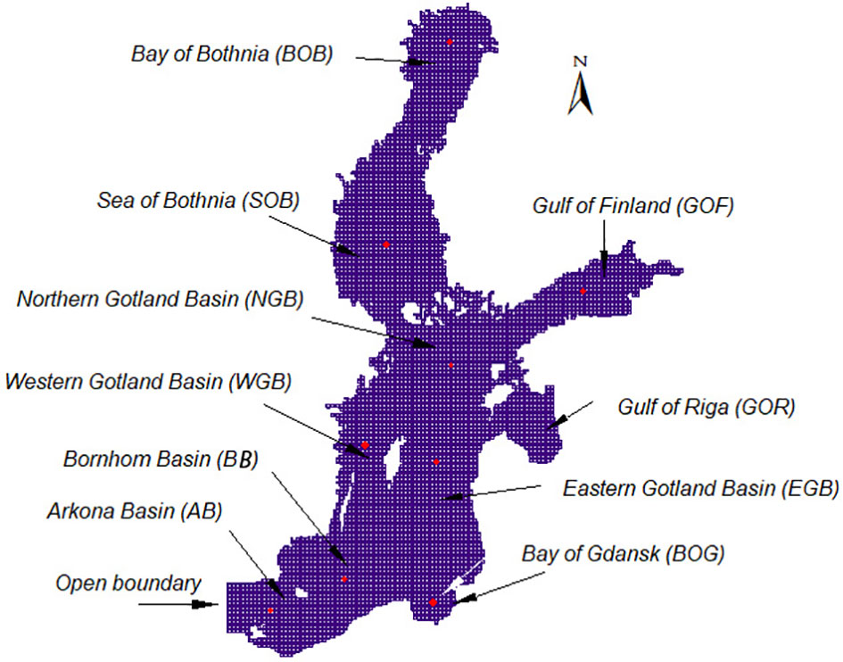
Figure 1 Hydrodynamic model mesh of the Baltic Sea with its deepest points in each basin marked by a red disc.
The temperature and salinity profiles measured at several locations in the Baltic Sea were used to calibrate the model for 2000. The restart files generated by the calibration simulation for 2000 were used to validate the model for ten years. Complete sets of profile field data from all monitoring sites were used. At all monitoring stations, model predictions of water temperature, salinity, and volumetric exchange rates with the North Sea were excellent. The Nash– Sutcliffe coefficients calculated for all monitoring sites ranged from 0.72 to 0.83. Another significant characteristic was the model’s capacity to capture 10-year seasonal fluctuations in water temperature and salinity with maximum relative accuracy of ±10%.
The use of particle tracking to investigate the dynamics of sediment transport in various flow regimes is a fairly well-established method. Krestenitis et al. (2007) and Israel et al. (2017) are examples of this approach. Krestenitis et al. (2007) investigated the sediment transport in the Gulf of Thermaikos, which constitutes the northwestern corner of the Aegean Sea. The model allowed investigation of patterns of sedimentary plume propagation existing in coastal systems. Concentrations of particles were deduced based on the particle mass and location. Israel et al. (2017) recently demonstrated the application of light particle tracking to simulate sediment transport loads in rivers. Their simulations were done using 350,000 particles, allowing for the determination of distinct hydrodynamic situations in which the zones are vulnerable to erosion and siltation at the port entrance in the Magdalena River, Colombia.
The three-dimensional PTM used in this study accounted for both the advection and dispersion processes of massless particles. Appendix A provides the model details. The model was used to simulate spatial and temporal variations in the sediment particle suspension that could not be extracted from the 2D sediment transport model directly. The paths of 1000 particles released from the deepest points in all 12 basins of the Baltic Sea (see Figure 1 for locations), were obtained for a 10-year simulation time (2000-2009).
The formulation of a comprehensive sediment transport model for the Baltic Sea was beyond the scope of this study. The main problems are the inherent empirical nature of the sediment transport equations and unknown boundary conditions. The first is related to the complex nature of interacting sediments with the flow, which does not allow the development of theoretically based equations. Second, such a model would require fully defined river inflow and sediment boundary conditions as well as lateral sediment boundary conditions. The latter consists of fine and often cohesive sediments (i.e., wash load) that enter the sea from the surrounding land by surface land erosion. In rivers, the load can be ignored because it is transported through the river and deposited downstream. The main difficulty is the lack of field data on sediment loads carried by rivers that discharge into the Baltic Sea. There is also no data available on the exchange rate of sediment transport at the model open boundary of the Danish Straits. In this study, a simplified two-dimensional (2D) approach was adopted, which served as the main objective of conducting a comparative study of the impact of SWM on background near-bed sediment concentrations in the Baltic Sea. It was further assumed that the equilibrium state of sediment transport prevailed in the Baltic Sea.
The model was used to simulate the spreading of sediment concentration close to the seabed. Sediment continuity equations for bed-level variations and suspended sediment transport equations were numerically solved. The two-dimensional (2D) form of the Exner equation is given by
where η is the bed elevation, λp is the porosity of the bed material, ca is the volume concentration of suspended sediment at the reference level, qbx and qby are the bed load transports in the x-y directions, ws is the particle settling velocity, and E is the volume rate of entrainment of sediment into the suspension, expressed as a fraction of T (dimensionless bed shear parameter, see Appendix B). In equation 1, ws ca denotes the volume flux of suspended sediment settling on the bed and ws E denotes the volume flux of entrainment of bed sediment into suspension, bed elevation increases due to the net deposition of suspended sediment if ca > E. To account for the influence of flocculation, the particle settling velocity for the cohesive sediment was estimated from the charts provided by Burt (1986) as a function of salinity and sediment concentration. The advection-diffusion equation for suspended sediment transport equation reads (2):
where C is the sediment concentration; u and v are the flow velocities in the XY directions, and εsx and εsy are the sediment diffusion coefficients in the XY directions.
The 2D equations were solved in the XY directions using a finite-difference approach and the Crank-Nicolson scheme (Dargahi, 2004; Shallal and Jumaa, 2016). The sediment diffusion coefficients were obtained from Van Rijn (1993) equations as a function of the shear velocity, flow depth, and settling sediment velocity. Furthermore, the coefficients were assumed to be equal in the x and y directions. These equations were applied to a unit layer above the seabed to obtain the maximum suspended sediment load, which was the focus of the SSTM model. Reference levels (a) were computed from Van Rijn (1993) relationship as a function of sediment size, that is, D50, D90 and shear stresses. A mean value of 0.1 m was used in all simulations.
The model required values for near-bed suspended sediment concentration (ca), bed load, and suspended sediment transport capacity at all mesh points. Modelling the foregoing parameters presents a real challenge owing to the semi-empirical nature of sediment transport equations, which are mainly based on flume tests. For these models to be useful, they must be verified using field measurements. In this study, the Van Rijn equations were used because of their wide range of applicability and good validation results. These equations have been reported to yield results that are closest to the field data (see Van Rijn, 1993). Sediment transport capacities were computed for non-cohesive and cohesive soils used in different basins of the Baltic Sea, which contain both soil types. For this purpose, Van Rijn (1993) approach and parameterization formulation for erosion flux were applied, as detailed in the previous paragraphs and Appendix B. The main inputs to the model were sediment size, sediment density, particle settling velocity, and flow characteristics (i.e., flow depth, flow velocity, and bed shear stress). The hydrodynamic model provided the flow velocities and bed shear stresses for the 10-year simulation period. The transient sediment model is decoupled from the hydrodynamic model. The shear stresses and velocities of the hydrodynamic model were used to compute suspended sediment transport at each time step. The SSTM used the non-cohesive and cohesive sediment sizes reported by Bobertz et al. (2005) in the Baltic Sea basins in agreement with their reported bottom sediment map. They reported the mean sediment sizes of silt = 20 μm, fine sand = 130 μm, and medium sand = 250 μm. They also provided data on the critical shear velocities for each sediment type as 4 cm/s, 1.4 cm/s, and 1.6 cm/s, respectively.
In the northern basins with cohesive soil types, the standard range of particle sizes was used, that is, silty clay (0.03-002 mm) and clay (0.001-0.0005 mm). The densities of sand, silt, and clay were 2082 kg/m3, 1300 kg/m3, and 1300 kg/m3 for wet-packed sand, silt, and clay, respectively. Seawater density and viscosity were obtained as functions of water temperature, salinity, and pressure. The computation of cohesive sediment transport (i.e. the rate of erosion) at the bed was done using the classical parameterization formulation for the erosion flux (Partheniades, 1965; Krestenitis et al., 2007 and Partheniades, 2009). Appendix B provides the details of the sediment transport equations used in this study.
No data were available on the sediment loads supplied by the rivers to the Baltic Sea. Thus, the boundary condition for the sediment transport model was set as a net sediment flux of zero.
The SWMM model aimed to investigate the suspension and dispersion of the increased suspended sediment load by the operation of the SWM collector (polymetallic nodules) within a one-meter layer of the seabed.
The main difficulty was to replicate the flow characteristics at the seabed realistically induced by the mining operation (i.e. collector). There is limited literature data on seabed mining that is mainly obtained from CFD simulations and small-scale and a few full-scale tests (Hengling and Shaojun, 2020; Chung 2021; Alhaddad et al., 2022; Muñoz-Royo et al., 2022). However, these data apply only to deep-sea cases and cannot be applied directly to the shallow waters of the Baltic Sea. Presently, no accessible information is available on the type of technology to be utilized in the Baltic Sea.
The Lagrangian spreading formulation for a plume (Lee and Chu, 2003; Elerian et al., 2021) was used to estimate the mean flow field characteristics induced by a collector. The formulation is based on the momentum and mass conservation equations. The discharge characteristics were taken as a velocity of 3 m/s, diameter of 0.25 m and collector speed of 0.25 m/s. These values were based on information available on various types of nodule mining systems (e.g. Elerian et al., 2021). According to this plume calculation, the mean entrainment conditions occurred at a velocity of 0.15 m/s and a bed shear stress of 6.35 N/m2 using the silt-clay density. The latter sediment type is the bed type found at the selected SWM locations in the Baltic Sea (see Figure 1 for locations). The collector with a speed of 0.25 m/s covers an area of about 4.6 km2 in one day. The selected variables were mining area within a mesh unit of 3.8x3.8 km, flow velocity 0.15 m/s and shear stress 6.35 N/m2. The SWMM used the cohesive sediment transport model that requires only the value of applied shear stress. Furthermore, it was assumed that the SWM collector operated at the deepest locations in the Baltic Sea. The model was applied to all 12 basins in the Baltic Sea, as shown in Figure 1, where the SWM locations are marked by small circles. The sediment transport computations were then repeated with the increased shear stress value. The shear stress was applied to the sediment transport model on the first day during the first month of each summer for the years 2000-2009 using dynamically set time steps.
The strength of the proposed model lies in its generality that neither required a presumed penetration depth nor the type of collector or machinery that may be applied to the case of the Baltic Sea.
The validation process of the suspended sediment transport model was based on the field data published by Ohde et al. (2007). In-situ measured suspended loads were reported for 2002 for the Arkona, Bornholm, and Gotland basins (see Figure 1 for locations). The sediment transport model was run in 2002 to obtain suspended sediment loads close to the seabed. The model was run for different sets of input parameters to obtain the closest agreement with field data. The main input parameters for the model were sediment size characteristics and density, sediment critical shear stress, and erosion rate parameters for cohesive soil (Ml). The non-cohesive sediment sizes D50 (Bobertz et al., 2005) were kept constant, whereas the range of variation for the cohesive material was silt-clay (0.03-002 mm) and clay (0.001-0.0005 mm). The sediment densities varied by ±10 of 2082 kg/m3, and 1300 kg/m3 for the non-cohesive and cohesive soils, respectively. The sediment critical shear values (τc) were obtained from the Shield Diagram as functions of the boundary Reynolds number (Re*). The diagram is valid in the range of 0.1< Re*<1000. The simulated minimum value of Re* is 0.2, which is within this range. The values of τc changed only slightly, that is, by 5% of the value found in the shield diagram for each D50 size. The validation process involved many transient sediment transport simulations to cover the range of input parameters. The input parameters are listed in Table 1.

Table 1 Validation sediment parameters for 2002.
Table 2 compares the 2002 simulated SSC (suspended sediment concentration) values with the 2002 in-situ measurements for the three basins of the Baltic Sea (Kyryliuk and Kratzer, 2019). It could not be determined with certainty when the measurements were taken, or the details of the actual method. They appear to have been taken from August 16 to September 3, 2002, which is late summer. The range of average values for the autumn period was closest to the measurements. However, the upper value for the Gotland Basin was overestimated by a factor of 1.5.
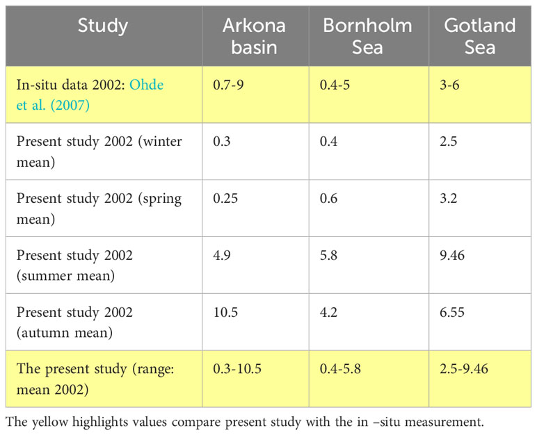
Table 2 Comparison of in-site and simulated SCC (g/m3).
The SSTM could not be fully validated due to a lack of sufficient field data on sediment concentrations as a time series across the Baltic Sea basins. Because of this constraint, the model was only used for a comparative study of the impact of seabed mining on sediment concentrations near the seafloor. Many inaccuracies exist in the actual measurements and the empirical nature of sediment transport equations, which are addressed in the discussion section.
The instantaneous hydrodynamic outputs were obtained daily during the 10-year simulation period. The outputs consisted of bed shear stresses and suspended sediment loads with and without SWM at the seabed. MATLAB was used to process the data and to create various contours and map plots. The daily model outputs were used to create 7,200 plots for the bed shear stresses and suspended loads and 210 plots for the SWMM simulations. The results and discussion are based on these plots and actual numerical values. An attempt was made to illustrate the results through a few typical representative plots.
The bed shear stresses exhibited significant spatial and seasonal variations in the range of 0.1-1.8 N/m2. Shear stresses were higher in the Gotland Basin than in other basins of the Baltic Sea. The maximum values were attained during late summer and autumn. The minimum values were in winter periods in the range of 0.01-0.5 N/m2. It should be noted that during the winter to early spring periods, the northern basins in the Baltic Sea were covered by ice, which explains the lower shear stress values. Figures 2 and 3 show summary plots of the average winter and summer periods for the years 2000, 2003, 2006, and 2009. The average values were for 21 days from January 20 to February 9 and June 29 to July 19. The figure clearly shows two important features: significantly reduced shear stresses in winter, and consistently higher shear stresses in the Gotland Basin throughout the year. Figure 2 depicts a significant rise in bed shear stress over the winter of 2009. One probable cause is the negative trend in ice cover formation throughout the 2000-decade period. Early in the year 2000, the upper basins of the Baltic Sea were regularly covered by a thick ice sheet (i.e., 30-80 cm). The southern basins were also close to freezing point. Because there is no ice cover, the wind can reach deep into the sea and thereby increase the bed shear stresses. The discussion section contains further information.
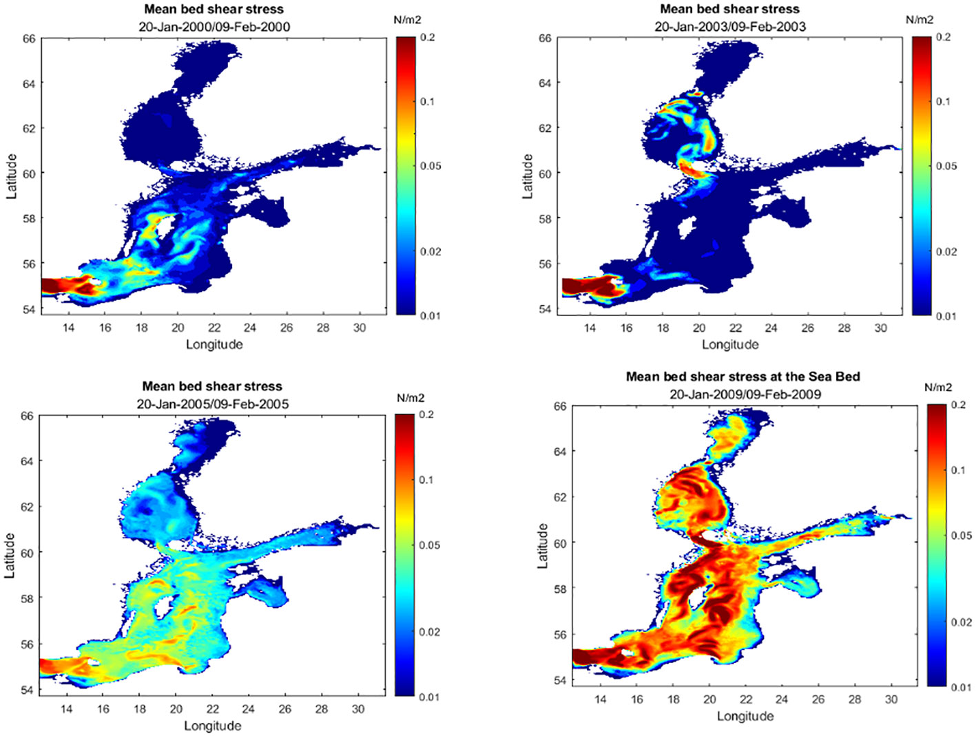
Figure 2 Filled contours of bed shear stress showing mean winter values in 2000, 2003, 2005, & 2009 (January 20- February 9).

Figure 3 Filled contours of bed shear stress showing mean summer values in 2000, 2003, 2005, & 2009 (June 29 – July 19).
According to the model results, suspended sediment transport is the primary transport mode, which is about ten times greater than bed load transport in all Baltic Sea basins. The mean value during summer periods is about 10-6 m3/m/s (volumetric rate per meter width) with higher values occurring in autumn and in the southern basins of the Baltic Sea. Aside from a few studies along the coast, there are no measurements of bed load transport in the open sea of the Baltic Sea. The preceding result can be addressed by reference to the measurements of bed load transportation taken over a 10-kilometer stretch of the southern Baltic Sea coastline (Krek et al., 2016). The mean recorded bed load was 23.8 kg, which may be converted to volume metric units using a density of 1200 kg/m3. It gives a value of 2.85x10⁻⁶ m3/m, which is consistent with the current finding. However, due to the differences between coastal and open sea bed load transport modes, this good agreement is inconclusive. As a result, the comparison should be interpreted only as an analysis of order of magnitude. Variations in the mean bed level elevations were ±1 mm, suggesting a state of dynamic equilibrium for the sediment transport. The model results indicated no significant imbalance in the erosion-deposition patterns for the 10-year simulation period. During winter, the bed-level variations were negligible.
Tables 3A, B list concentration statistics for a 3-year period of 2007-9 where the minimum and maximum seasonal values are given. The maximum suspended sediment concentrations for the simulated period varied in the range of 0.1-90 g/m3. The range corresponds to sediment concentrations during winter and the first month of autumn, respectively. In analogy with the bed shear distributions, the loads showed significant spatial and temporal variations. Higher values were found in the Gotland basins (see Figure 1 for locations) during warmer periods of the year. The foregoing result agrees with the data reported by Kyryliuk and Kratzer (2019). The winter periods had the lowest values typically 0.1-1 g/m3. To illustrate some of the main features, Figure 4 shows four plots of the 21-day averaged values of suspended loads for winter and spring for the years 2005 and 2009. The mean concentrations were found to be generally higher in 2009 (see Figure 4). Figure 5 shows four plots of the 21-day averaged values of suspended loads for summer and autumn for the years 2005 and 2009. The mean values during winter and spring periods were < 0.3 g/m3, and 0.5-4 g/m3, respectively. Much higher concentrations occurred during the summer and autumn. The corresponding ranges were 1-8 g/m3 and 2-12 g/m3. However, maximum values increased by a factor of 10 between winter and summer. Figures 6A, B show a typical plot of the higher sediment concentrations and the corresponding bed shear stresses on October 9, 2009, respectively. Significantly increased concentrations and shear stresses are noticeable in the Arkona Basin which propagates a considerable distance into the Bornholm Basin. The increased concentrations could be correlated with high water levels at the open boundary of the model that correspond to inflow events from the North Sea with a typical time scale in the range of 1-7 days that normally occur during late summer and autumn periods (see Mohrholz, 2018; Dargahi, 2022).
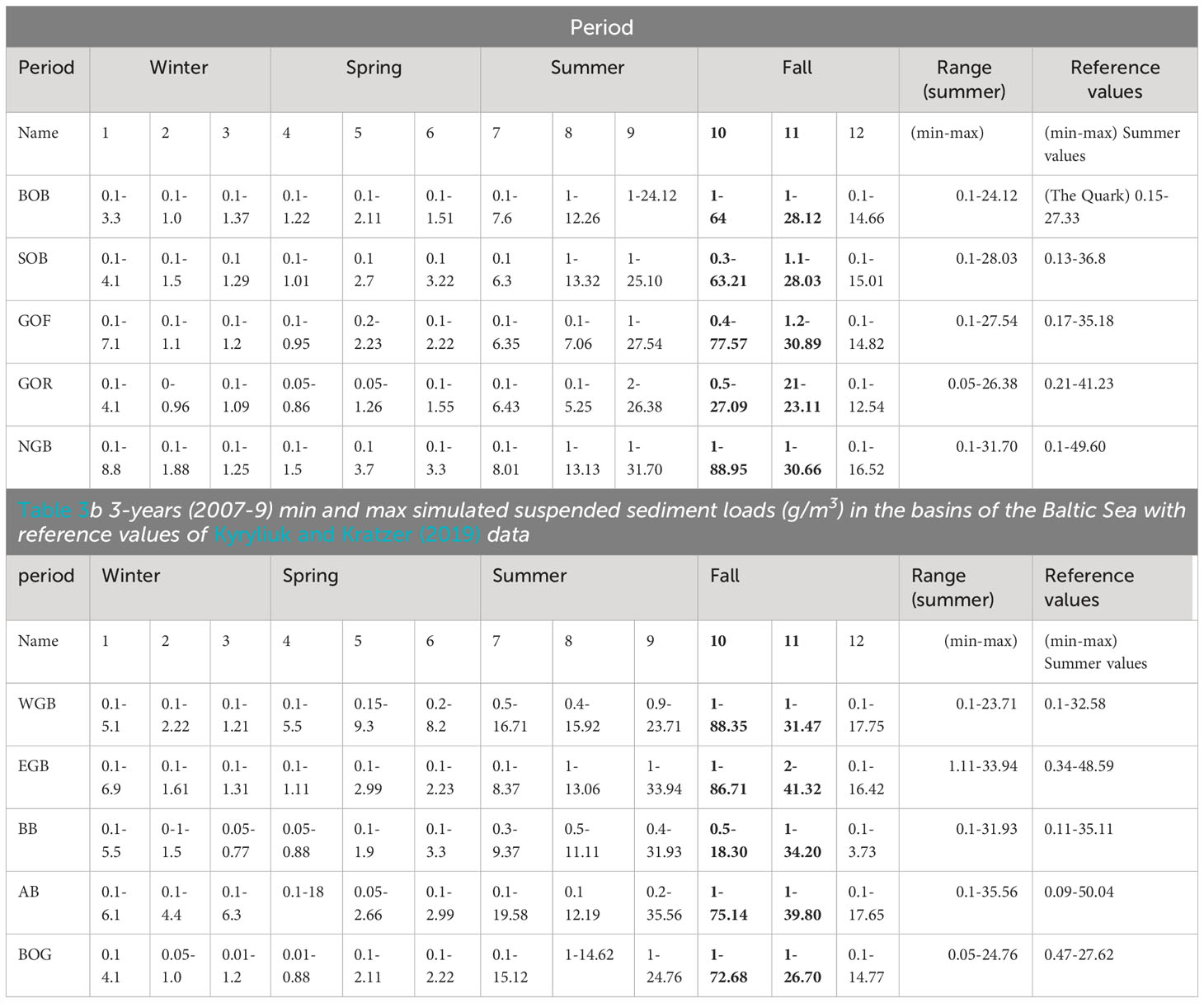
Table 3 3-years (2007-9) min and max simulated suspended sediment loads (g/m3) in the basins of the Baltic Sea with reference values of Kyryliuk and Kratzer (2019) data.

Figure 4 Filled contours of mean sediment concentrations in the Baltic Sea, winter (January 21-Feburary 10) and spring (April 26-May 19), 2005 & 2009.
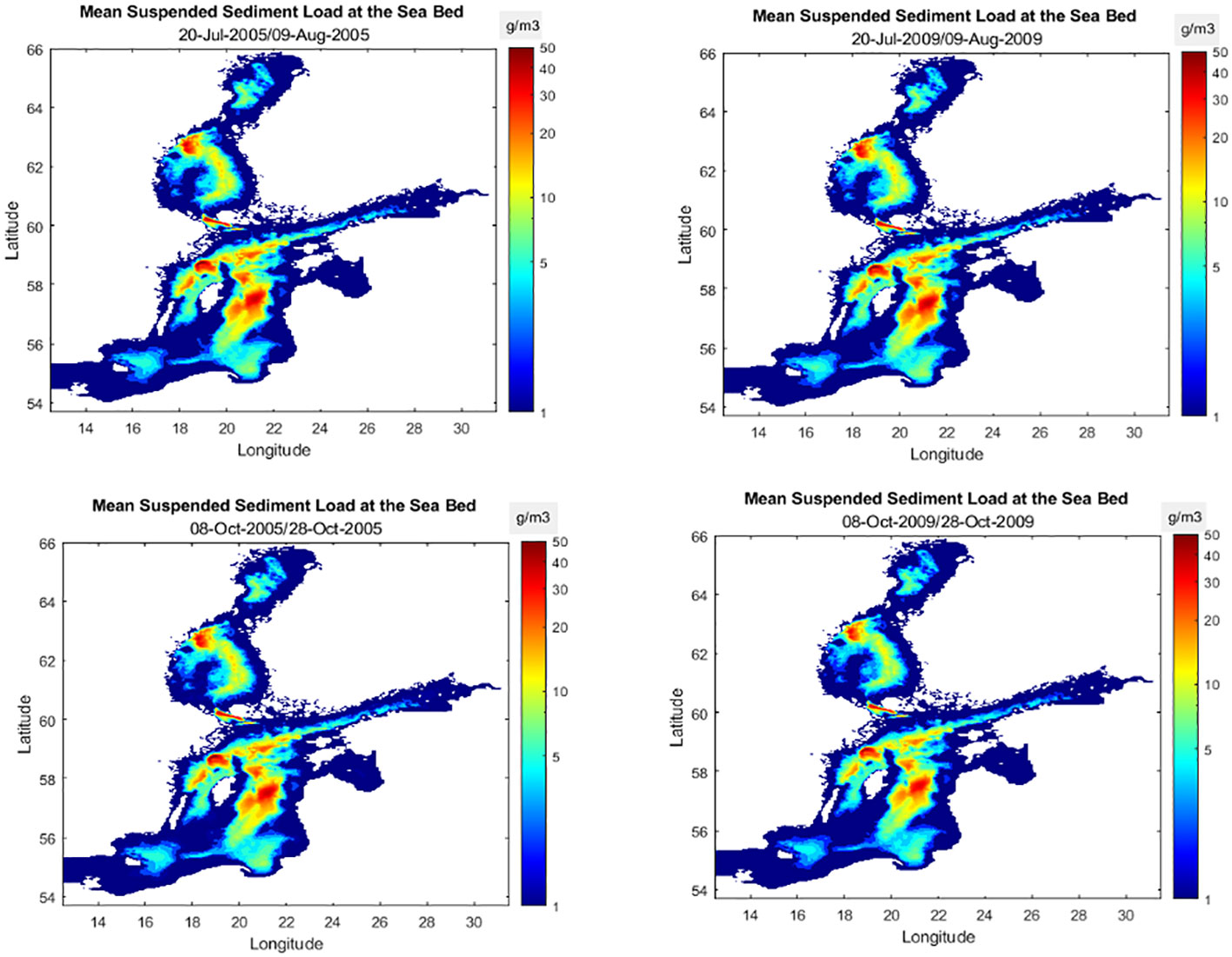
Figure 5 Filled contours of mean sediment concentrations in the Baltic Sea, summer (July 20-August 9) and autumn (October 8-28), 2005 & 2009).
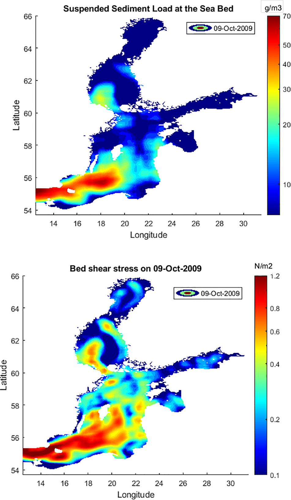
Figure 6 Filled contours of instantaneous sediment concentrations and bed shear stresses on Oct 9, 2009.
The simulated effect of SWM on sediment suspension showed significant temporal and spatial variations from basin to basin. The sediment concentration increased by several factors compared with the background equilibrium conditions. The range of maximum values was 300-500 g/m3 at the simulated mining locations, which corresponded to one model mesh of 3.8 x 3.8 km. The upper range was detected mainly in the Gotland Basin. The decay rate of sediment concentrations ranged from 10 to 14 g/m3 per day, showing a slower decay in the northern basins of the Baltic Sea. Typically, the concentration of 350 g/m3 decreased to 100 g/m3 in the southern basins and 150 g/m3 in the northern basins. These values were well above the background sediment concentration. The high-concentration regions were mostly limited to mining areas, although their magnitude decreased over time.
The immediate area affected was approximately 7.6 x 7.6 km, i.e. 2 times the mining area. The main features are illustrated in a set of plots (Figures 7 and 8). They show the filled contours of suspended sediment concentrations at the start of mining on June 28, 2009, in five basins of the Baltic Sea (BOB, GOF, EGB, WGB, see Figure 1). The velocity vectors at the intervals of the four meshes are overlaid. Suspended sediment loads are transported to large areas around the mining locations in the direction of the local velocity field. In the southern basins, the sediment spread to larger areas and exhibited a faster decay in sediment concentration than in the northern basins of the Baltic Sea. Figure 9 shows the decay profile of the maximum concentration in WBG during the same period. The upper and lower curves represent the sum of SWM induced and background loads, and background loads, respectively. Deducting the two preceding profiles yields the net SWM-induced load. The concentration after 21 days was still about 2 higher than the background maximum concentration. The variation in the local bed level elevations was ± 1 cm, which was ten times greater than the variation in the mean bed level without SWM (i.e., ± 0.1 cm). Figure 10 compares the background and total SWM (SWM plus background) bed level variations in WGB on June 29, 2000. The cross-section was taken at 57°8´ N - 17°87´E and 57°8´N - 18°52´E which is drawn with a white dashed line in Figure 8, WGB. The zero position refers to the center point of the mining region. The net SWM-induced profile can be obtained by deducting the two profiles.
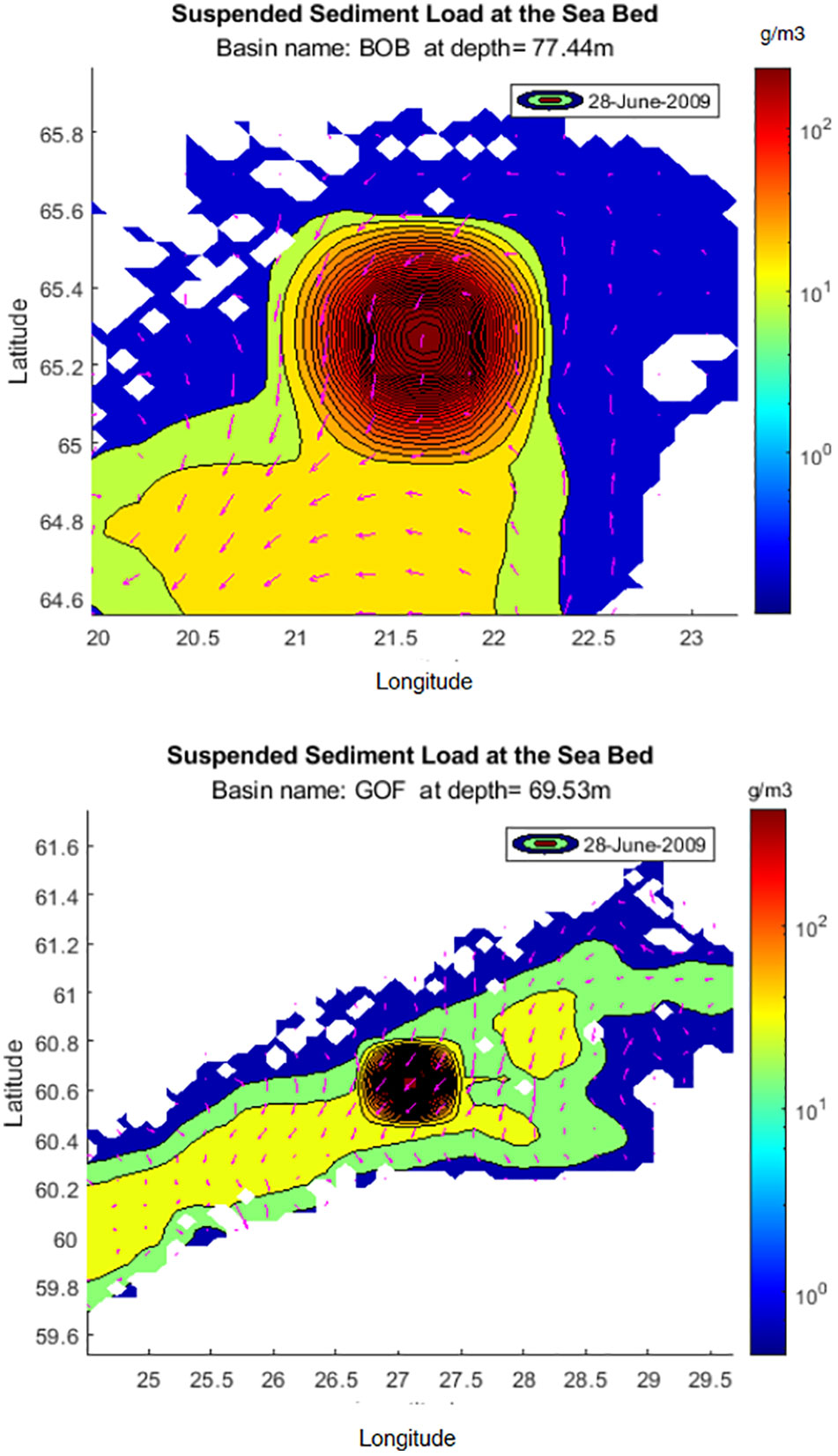
Figure 7 Filled contours of sediment concentrations at the start of SWM, on June 28, 2009, in basins: BOB &GOF.
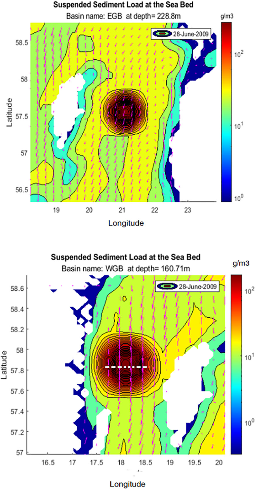
Figure 8 Filled contours of sediment concentrations at the start of SWM, on June 28, 2009, in basins: EGB & WGB (Cross-section marked by a white dashed line).
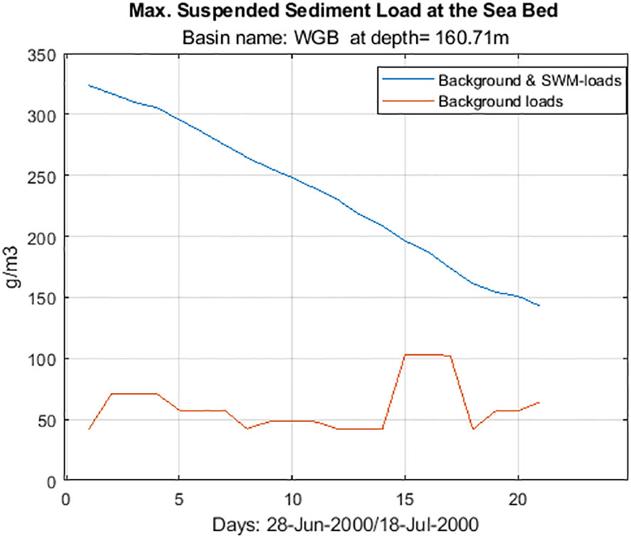
Figure 9 Decay of maximum sediment concentrations in WGB, June 28-July 18, 2000.

Figure 10 Comparison of background and combined SWM-induced and background bed level variations in WGB, June 29, 2000. The cross-section taken at 57°8´N - 17°87´E, 57°8´N - 18°52´E.
The particle tracking results provided insights into the spatial and temporal variations in the suspension of sediment particles. The main aspects to be considered were the Lagrangian spreading of particles, final particle concentrations, and timescales. Generally, particles follow complicated patterns driven by general circulation patterns, secondary flow patterns, and mesoscale vortices (Dargahi, 2022). There are three general circulation patterns in the Baltic Sea: anticlockwise circulation in the upper water layers, clockwise circulation in deeper regions, and cyclonic circulation around the Gotland Island, which is the main circulation pattern in the Gotland Basin. Typical results for the two basins are shown in Figure 11 for BOB and WGB (see Figure 1 for locations). They show plane views of the particle paths colored according to the depth. These figures correspond to the 10-year simulation period. Table 4 summarizes the main results.
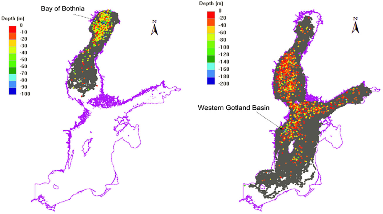
Figure 11 Particle paths in different basins of the Baltic Sea colored by depths in two basins: BOB and WGB. Period 2000-2009.
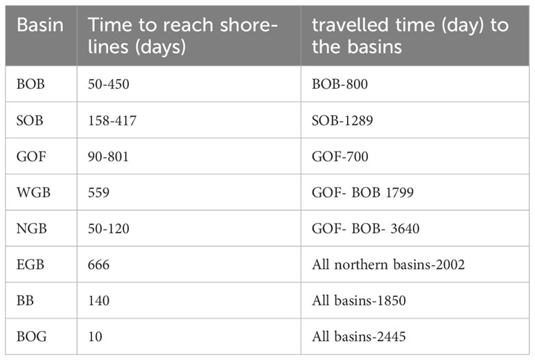
Table 4 Particle tracking travel times to shorelines and time to reach the farthest basin.
Most particles in the three northern basins (BOB, SOB, and GOF, see Figure 1 for locations) remained within the respective basins, with timescales of 700-1289 days. After a simulation period of 3650 days, 30% of the particles reached the thermocline layers at approximately half the time scale. The range of the maximum distance travelled was 700-1000 km.
The particles released in the other western basins (BB and BOG) spread to most of the basins in the Baltic Sea, covering the longest distances of up to 1300 km. In these basins, 60% of the particles reached the thermocline layers after 200-350 days. The results indicate a significant difference between the northern and southern basins of the Baltic Sea in terms of both time and length scales. Interpolation of the foregoing results for the dispersion of suspended sediment is presented in the discussion section.
There are limitations in both hydrodynamic and sediment transport models. The fully validated 3D hydrodynamic model showed good performance in comparison with the measured thermodynamic properties of the sea and the recorded water levels, with a maximum error of 10%. However, increasing the vertical resolution of the model produces more detailed and accurate results. The choice of the present model size was limited by the available CPU. The 2D sediment transport model provides the general pattern of sediment transport and bed level variations, but it cannot resolve the 3D characteristics of sediment movements. The latter type of model is more accurate and representative of the prevailing complex flow patterns in the Baltic Sea. However, apart from serious numerical difficulties and a very long computation time, an extensive and detailed set of coherent field data is required to verify and validate the model. Presently, the required data are neither available nor are there any plans to collect them soon. The 2D sediment model is a good starting platform for examining the mean features of sediment transport and addressing the effect of seabed mining. The other aspect is that the shallow water model was based on the estimation of the applied shear stress based on physical principles. As stated in the SWMM section, no information was available to aid in the selection of more realistic values. However, one merit of the SWMM model is the selection of the applied shear stress was estimated independently of the type of mining machinery. The applied value of the shear stress induced by the collector is not unreasonable in comparison with the values reported in the literature. However, the study does not rule out alternative configurations.
There are several uncertainties inherent in the numerical modelling of sediment transport, owing to the semi-empirical nature and uncertainties of sediment data and their characteristics. Models of large water bodies such as the Baltic Sea encounter further difficulties because data on sediment loads are often unavailable at the inlet and outlet boundaries. The current model assumed zero net sediment flux, which did not require actual boundary values. This boundary condition can be understood as a state of dynamic equilibrium that ensures a balance between erosion and deposition. The validity of this assumption is discussed in terms of the study objective. The Baltic Sea is a semi-closed system that exchanges water and masses along its open boundary in the Danish Strait. The main sediment input is through rivers, which are balanced by outgoing sediment transport at the open boundary and the sediment rate of change within the sea. However, the main driving force for sediment transport is bed shear stress, which was obtained from the validated hydrodynamic model. The focus of this study was to compare two cases, with and without SWM, regarding seabed sediment concentrations. In both cases, the acting shear stress field was induced by the hydrodynamics of the sea and not by sediment transport boundary conditions. This implies that the comparison between the two cases was relatively independent of the sediment loads at the boundaries. Furthermore, the seabed elevation changes offshore of a large water body of the order of millimeters, which is several orders of magnitude smaller than the sea depth. This implies a negligible change in the flow field and bed shear stresses.
The sediment transport model of the Baltic Sea yielded sediment concentrations that were in reasonable general agreement with the reported data. However, an accurate comparison requires in-situ measurements of sediment concentrations near the seabed, which are currently unavailable. The present data are Kyryliuk and Kratzer (2019) satellite-based data and in-situ data obtained from previous studies mainly in the summer of 2002. Tables 3A, B show the 3-year (2007-9) min and maximum simulated suspended sediment loads (g/m3) in the basins of the Baltic Sea and the reference values of Kyryliuk and Kratzer (2019). There is a general agreement regarding the range of the min-max data in summer periods. However, the maximum values obtained in this study are approximately 20% lower. Kyryliuk and Kratzer stated that, for each basin, their satellite data showed a much higher range than the reported in situ range. There are several possible explanations for the deviation between the two datasets. Generally, measuring the maximum values is associated with higher uncertainties and errors depending on the length and duration of the data and the time of measurement. Kyryliuk and Kratzer’s data are associated with some additional uncertainties. The data were derived from satellite information obtained using NASA MERIS ocean color sensing and optical transect measurements, which are often dominated by organic matter rather than actual suspended matter. Furthermore, satellite-based data cannot resolve the higher near-seabed sediment concentrations, which is one of the major shortcomings of the method. The details of these satellite-based data regarding the accuracy, exact time, and locations of the measurements are also unclear. Presently, taking extensive sediment concentration measurements in large and deep water bodies is technically and economically not feasible.
Despite these shortcomings, numerical models yield results that cannot be obtained using a limited number of measurements. This is especially true for large open-water bodies such as the Baltic Sea.
The results are discussed with a focus on two important aspects. One is the state of near-bed sediment concentrations and bed level variations for the decade 2000-2009. The second is the change induced by SWM in near-bed sediment concentrations and the bed level variations (i.e. erosion-deposition).
The instantaneous concentrations in the Baltic Sea showed significant seasonal and spatial variations, analogous to bed shear stress, as indicated in the previous sections. The occurrence of higher concentrations during the late summer-autumn period correlated with increased westerly wind conditions during the same period. During the simulation period, the maximum measured wind speed range was 20-30 m/s. These wind speeds are sufficiently high to reach maximum depths in most basins of the Baltic Sea, inducing higher shear stress and thus increasing sediment transport. Generally, the winds were approximately 1.5-2 higher in the Gotland basins (see Figure 1 for locations), which could explain the higher shear stress and sediment loads in these basins in comparison with the northern basins. In winter, there is a considerable reduction in the shear stress at the seabed and sediment transport activities. This can be attributed to the formation of ice cover in the northern basins and the moderately reduced meteorological loading, specifically wind speed, throughout the basins. Contrary to the significant seasonal variations in sediment concentrations, there was little annual change in sediment concentrations during the period 2000-2008. Sediment concentrations were reduced throughout the winter because the ice cover effectively inhibited wind force from acting on the flow. The formation of ice significantly alters the flow dynamics by converting it into a closed conduit. The vertical shear stress distribution changes to a parabolic profile that divides the total shear stress between the seabed and under the ice cover. The amount of shear stress applied to each surface is determined by the roughness ratio of the ice cover and the seabed. This means that when there is no ice cover, all shear loads are applied to the bottom, increasing sediment concentrations in comparison to ice-cover years. Higher sediment concentrations during the winter of 2009 can be explained by changing ice conditions. The alarming decline in ice conditions has persisted until 2022. Rapid climate change could be the main reason for the altered ice conditions in the Baltic Sea.
Higher values of background sediment concentrations during the summer and early fall seasons may be related to the enhanced forcing meteorological circumstances, particularly wind speed. Figure 12 illustrates the correlation by comparing the evolutions of sediment concentrations with wind speeds in WGB at grid position with depth 160.71 in 2009 (the net SWM-induced loads are also plotted in the same figure). Sediment concentrations increase as wind speed increases, and both variables are characterized by a third-degree polynomial.
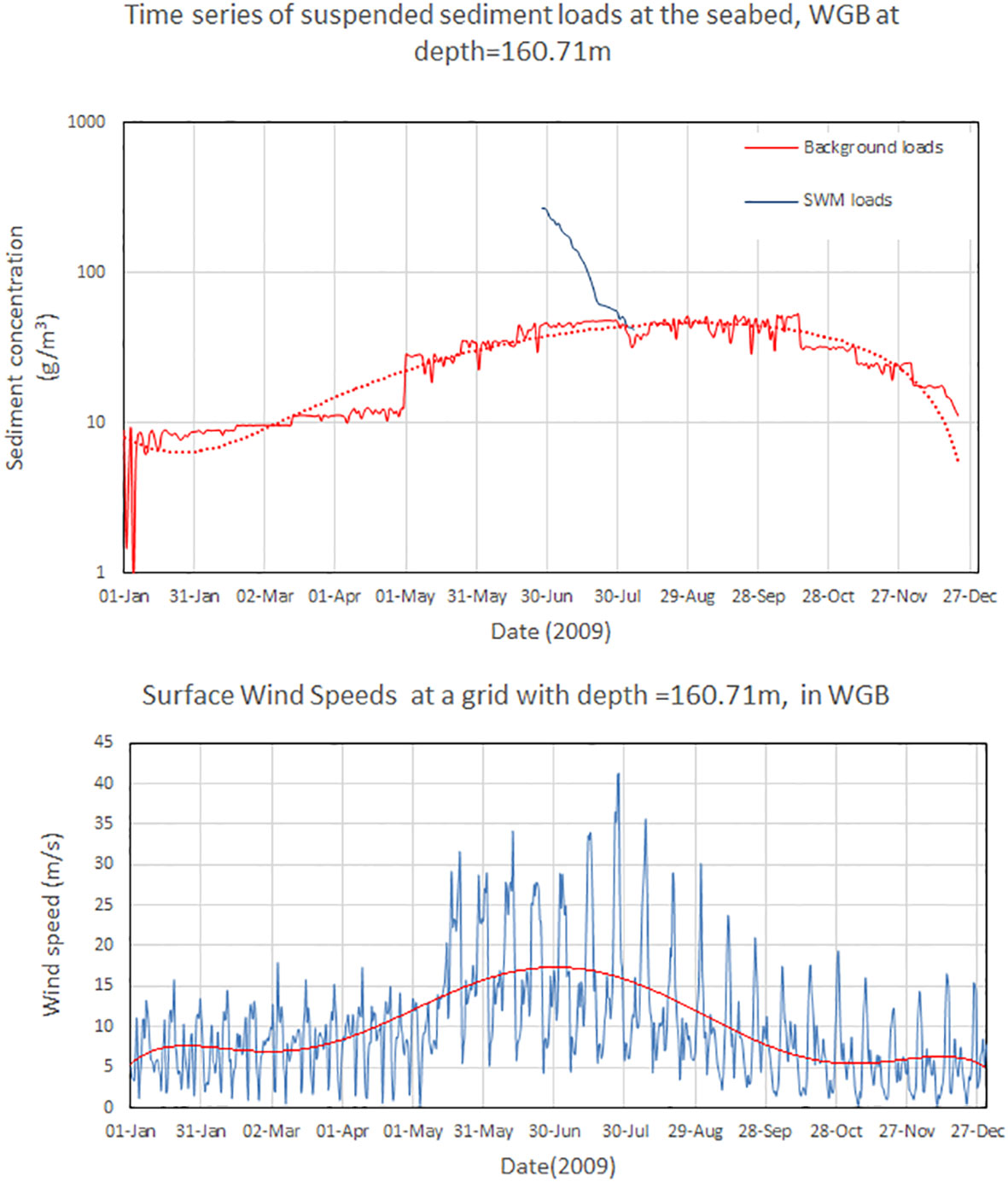
Figure 12 Time series of suspended sediment concentration of background and SWM induced loads and wind speeds in 2009, Western Gotland Basin, at the grid with depth 160.71 m.
Regarding the impact of SWM, there are three important aspects of sediment concentrations, the decay rates and bed-level variations induced by the collector.
High sediment concentrations adversely affect marine habitats. DFO (2000) provides guidelines for protecting fishery resources in terms of sediment concentration risk levels of sediment concentration. The classified risk levels of concentration were low risk 25-100 g/m3, moderate risk 100-200, high risk 200-400, and unacceptable (> 400 g/m3). In the case of SWM, the maximum concentrations were 300-500 g/m3 which are within the high and unacceptable risk levels. This yielded an increase in concentration by a factor of 3-5 in comparison with the maximum background concentrations.
The decay rates were in the range of 10-14 g/m3 per day in the northern and western basins of the Baltic Sea. The weaker flow field and the difference in the sediment properties in the former basins explain the slower decay (see Figure 9). However, the final decay time to the background levels is approximately 40 days which gives a decay rate of approximately 7.5 g/m3 per day (see Figure 12). The results indicate that the region affected by SWM was limited to ±15 km which is approximately four times the mining area, as shown in Figure 10. However, the impact should be understood in terms of bed-level variations that nearly coincide with the background bed levels within a distance of ±15 km. The net SWM-induced loads are also plotted in the same figure.
Because of the active transport of suspended sediments by currents, the real region affected by SWM may be substantially larger than described by bed level variations. In comparison to silt and sand, cohesive sediments have a very low settling velocity in the absence of flocculation, which keeps the material afloat for extended periods. The creation of coarser aggregates may change their settling velocity and aid in the reduction of mining plume spread, especially in the deep sea, where the surficial sediment is mostly solid clayey sediment (Gillard et al., 2019; Ali et al., 2022). In the former case, the cohesive material could travel further before settling on the seabed. This trend can be confirmed by data reported by Ryabchuk et al. (2017) and the PTM. They reported that during construction work in Neva Bay, fine sediments were transported into the GOF (see Figure 1 for locations) up to tens of kilometers off the coast. The tenfold bed level changes induced by SWM suggest that harmful substances, such as heavy metals have the potential of being transported and spread to all basins.
The various limitations of the sediment transport model did not allow investigation of the dynamics of the sediment transport and its 3D nature in the Baltic. However, the particle-tracking model provided useful information on the spatial and temporal characteristics of suspended sediment particles in water.
The applied model accounted for both the advection and dispersion of massless particles. The SSTM accounted for sediment particles larger than 0.005 mm, i.e., very fine silt to coarse clay, with a mean density of 1200 kg/m3. However, the density of the suspended cohesive material can be as low as 1130 kg/m3 which is close to that of seawater 1025 kg/m3. This implies that massless particles provide a reasonable representation of the advection and dispersion of particles with these characteristics. However, compared to heavier particles in the suspension, the dynamic properties of these particles are overestimated in comparison with those of small mass. The limitation on the density implies the spreading of the plume to larger areas.
The particle-tracking model suggested the extensive spreading of particles within all basins of the Baltic Sea. In the southern basins, with strong secondary flows, particles spread into the northern basins over a timescale of 5-7 years. In the southern basins, the particles could reach the shorelines within a relatively short time interval of 10 days to 2 years, and the model-predicted time scale to reach the thermocline layers ranged from 30% to 60% of the total particles released in the northern and southern basins, respectively. The foregoing characteristics, with long spatial-temporal scales, provide some insight into the alarming possible spreading of dislodged particles from the seabed by SWM. The operation will also expose the containment materials which are stored at the top sediment layer of the seabed.
The proposed modelling schemes were developed for a comparative study of the impact of shallow water mining in the Baltic Sea.
The application of combined hydrodynamic, particle tracking, and sediment transport models to the Baltic Sea revealed important characteristics of near-bed suspended sediment concentrations.
The main undisturbed transport mode of the Baltic Sea is the suspended transport load, which spreads to all Baltic Sea basins. The advection timescale varied from 10 days to 7 years, depending on the shoreline and basin. The average sediment concentration was approximately 2 g/m3, with peaks up to 90 g/m3 on a single autumn day.
Shallow water mining significantly alters the equilibrium state of sediment transport in the Baltic Sea. The sediment concentrations could reach 300-500 g/m3, which are 3-5 times higher than the background sediment concentrations at the time of mining. These high values are classified as unacceptable risks to fishery resources and sea ecology. The size of the SWM-affected area concerning the bed-level changes was approximately 4 times that of the center point of the mining area. The PTM suggested extensive spreading of lighter particles to all the basins of the Baltic Sea with very large time and length scales. These particles could reach the thermocline layers with a mean concentration of 40%. SWM operation ten folded the bed level variations, posing an additional threat to the ecological health of the Baltic Sea by exposing the contaminated sediment to transport. The Gotland Basin in the Baltic Sea is most vulnerable to SWM.
The environmental and ecological risks of shallow water mining in the Baltic Sea are not sufficiently studied. Consequently, it is prudent to exercise caution and, until then, maintain the Baltic Sea seabed as a region free of mining.
The raw data supporting the conclusions of this article will be made available by the authors, without undue reservation.
I am the only author.
The author(s) declare that no financial support was received for the research, authorship, and/or publication of this article.
The greatest accomplishment of men is the scientific advancements for the good of humanity and nature. Freedom and liberty constitute the essence of this progress driven by thousands of men of science prevailing throughout centuries. Yet, in many parts of the world, there are dark totalitarian forces that deprive humanity of greater achievements through systematic abuse, imprisonment, and murder of fellow scientists and scholars. The author dedicates this work to the memory of all fellow scientists and students in Iran who have endured formidable anguish and lost their lives in the struggle for democracy and science. Thanks to the insightful comments and suggestions of the reviewers and editor, the manuscript was improved.
The author declares that the research was conducted in the absence of any commercial or financial relationships that could be construed as a potential conflict of interest.
All claims expressed in this article are solely those of the authors and do not necessarily represent those of their affiliated organizations, or those of the publisher, the editors and the reviewers. Any product that may be evaluated in this article, or claim that may be made by its manufacturer, is not guaranteed or endorsed by the publisher.
Ahnert A., Borowski C. (2000). Environmental risk assessment of anthropogenic activity in the deep-sea. J. Aquat. Ecosyst. Stress Recov. 7 (4), 299–315. doi: 10.1023/A:1009963912171
Alhaddad S., Methta D., Helmons R. (2022). Mining of Deep-Seabed Nodules Using a Coandă-Effect-Based Collector (Netherlands: Delft University of Technology). doi: 10.1016/j.rineng.2022.100852
Ali W., Enthoven D. H. B., Kirichek A., Helmons R. L. J., Chassagne C. (2022). “Can flocculation reduce the dispersion of deep sea sediment Plumes?,” in Proceedings of the World Dredging Conference, WODCON XXIII: Dredging is Changing (Copenhagen, Denmark: WODA).
Ansari T. M., Marr I. L., Tariq N. (2004). Heavy metals in marine pollution perspective–A mini review. J. Appl. Sci. 4, 1–20. doi: 10.3923/jas.2004.1.20
Bobertz B., Kuhrts C., Harff J., Fennel W., Seifert T., Bohling B. (2005). Sediment properties in the western Baltic Sea for the use in sediment transport modelling. J. Coast. Res. 21 (3), 588–597. doi: 10.2112/04-705A.1
Burt T. N. (1986). “Field settling velocity of estuary muds,” in Estuarine cohesive sediment dynamics lecture notes on coastal and estuarine studies. Ed. Mehta A. J. (New York, NY: Springer) vol. 14. doi: 10.1007/978-1-4612-4936-8_7
Byishimo P. (2018). Experiments and 3D CFD simulations of deep-sea mining plume dispersion and seabed interactions, Master of Science thesis (Netherlands: Delft University of Technology).
Dargahi B. (2004). Three-dimensional flow modelling and sediment transport in the River Klarälven. Earth Surf. Process. Landforms. 29, 821–852. doi: 10.1002/esp.1071
Dargahi B. (2022). Lagrangian coherent structures and hypoxia in the baltic sea. Dynamics. Atmospheres. Oceans. 97, 101286. doi: 10.1016/j.dynatmoce.2022.101286
Dargahi B., Cvetkovic V. (2014). Hydrodynamic and Transport Characterization of the Baltic Sea 2000-2009 (Stockholm, Sweden: KTH Royal Institute of Technology, TITA A-LWR). Report 2014:03, ISSN 1650-8610.
DFO (2000). “Effects of sediment on fish and their habitat,” in DFO Pacific Region Habitat Status Report 2000/01 E. Canada. Available at: https://waves-vagues.dfo-mpo.gc.ca/library-bibliotheque/255660.pdf.
Dimou N., Adams E. (1993). Random-walk particle tracking models for well-mixed estuaries and coastal waters. Estuar. Coast. Shelf. Sci. 99–110. doi: 10.1006/ecss.1993.1044
Earle S., Kammen D. (2022) The case against Deep-Sea Mining. Available at: https://rael.berkeley.edu/wp-content/uploads/2022/10/Earle-Kammen-The-Case-Against-Deep-Seabed-Mining-TIME-10-25-2022.pdf.
Elerian M., Alhaddad S., Helmons R., van Rhee C. (2021). Near-field analysis of turbidity flows generated by polymetallic nodule mining tools. Mining 1, 251–278. doi: 10.3390/mining1030017
Enerdata (2022). “World Energy and Climate Statistics – Yearbook 2022,” in World Energy Consumption Statistics, Enerdata.
Farran S. (2022). Deep-sea mining and the potential environmental cost of ‘going green’ in the Pacific. Environ. Law Rev. 24, (3). doi: 10.1177/1461452922111494
Gillard B., Purkiani K., Chatzievangelou D., Vink A., Iversen M. H., Thomsen L. (2019). Physical and hydrodynamic properties of deep sea mining-generated, abyssal sediment plumes in the Clarion Clipperton Fracture Zone (eastern-central Pacific). Elementa. Sci. Anthropocene. 7, 5. doi: 10.1525/elementa.343
Halfar J., Fujita R. M. (2007). Ecology: Danger of deep-sea mining. Science 316 (5827), 987. doi: 10.1126/science.1138289
HELCOM (2021) Inputs of hazardous substances to the Baltic Sea. Baltic Marine Environment Protection Commission, BSEP n°179 Helsinki Commission. Available at: https://helcom.fi/wp-content/uploads/2021/09/Inputs-of-hazardous-substances-to-the-Baltic-Sea.pdf.
Hengling Y., Shaojun L. (2020). A new lifting pump for deep-sea mining. J. Mar. Eng. Technol. 19 (2), 102–108. doi: 10.1080/20464177.2019.1709276
IEA (2022). Global Supply Chains of EV Batteries (Paris: IEA). Available at: https://www.iea.org/reports/global-supply-chains-of-ev-batteries.
Israel E. H., Franklin M. T., Jatziri Y. M. M., Rodriguez-Cuevas C., Couder-Castañeda C. (2017). Light particle tracking model for simulating bed sediment transport load in river areas. Math. Problems. Eng. 2017, 1679257. doi: 10.1155/2017/167925
IUCN (2022). “Deep-sea mining, International Union for Conservation of Nature,” in Issues brief Deep-Sea mining resource. (Gland, Switzerland: IUCN).
Jankowski J. A., Zielke W. (2001). The mesoscale sediment transport due to technical activities in the deep sea. Deep-Sea. Res. Part Trop. Studier. Oceanogr. 48 (17), 3487–3521. doi: 10.1016/S0967-0645(01)00054-6
Kaikkonen L., Virtanen E., Kostamo K., Lappalainen J., Kotilainen A. (2019). Extensive coverage of marine mineral concretions revealed in shallow shelf sea. Front. Mar. Sci. Section. Coast. Ocean. Processes. 6. doi: 10.3389/fmars.2019.00541
Krek A., Stont Z., Ulyanova M. (2016). Alongshore bed load transport in the southeastern part of the Baltic Sea under changing hydrometeorological conditions: Recent decadal data. Regional. Stud. Mar. Sci. 7, 81–87. doi: 10.1016/j.rsma.2016.05.011
Krestenitis Y. N., Kombiadou K. D., Savvidis Y. G. (2007). Modelling the cohesive sediment transport in the marine environment: the case of Thermaikos Gulf. Ocean. Sci. 3, 91–104. doi: 10.5194/os-3-91-2007
Kyryliuk D., Kratzer S. (2016). Total suspended matter derived from MERIS data as indicator for coastal processes in the Baltic Sea. Ocean. Sci. doi: 10.5194/os-2016-2
Kyryliuk D., Kratzer S. (2019). Summer distribution of total suspended matter across the baltic sea. Front. Mar. Sci. 5 (504). doi: 10.3389/fmars.2018.00504
Lee J. H., Chu V. H. (2003). Turbulent Jets and Plumes, A Lagrangian approach (Dordrecht, Netherlands: Kluwer Academic Publisher).
Mellor L., Yamada T. (1982). Development of a turbulence closure model for geophysical fluid problems. Rev. Geophys. 20 (4), 851–875. doi: 10.1029/RG020i004p00851
Miller K. A., Thompson K. F., Johnston P., Santillo D. (2018). An Overview of seabed mining including the current state of development, environmental impacts, and knowledge gaps, 10. Section. Deep-Sea. Environ. Ecol. 4. doi: 10.3389/fmars.2017.00418
Mohrholz V. (2018). Major baltic inflow statistics revised. Front. Mar. Sci. 22 Section Coastal Ocean Processes 5. doi: 10.3389/fmars.2018.00384
Muñoz-Royo C., Ouillon R., Mousadik S., Alford M. H., Peacock T. (2022). An in situ study of abyssal turbidity-current sediment plumes generated by a deep seabed polymetallic nodule mining preprototype collector vehicle. Sci. Adv. Oceanogr. 8. doi: 10.1126/sciadv.abn1219
NOAA (2020). Ocean pollution and marine debris (Washington, D.C.: National Oceanic and Atmospheric Administration, U.S. Department of Commerce).
Ohde T., Siegel H., Gerth M. (2007). Validation of MERIS Level-2 products in the Baltic Sea, the Namibian coastal area and the Atlantic Ocean. Int. J. Remote Sens. 28 (3-4), 609–624. doi: 10.1080/01431160600972961
Orcutt B. N., Bradley J. A., Brazelton W. J., Estes E. R., Goordial J. M., Huber J. A., et al. (2020). Impacts of deep-sea mining on microbial ecosystem services. Limnol. Oceanogr. 65, (7). doi: 10.1002/lno.11403
Partheniades E. (1965). Erosion and deposition of cohesive soils. J. Hydraulic. Division. ASCE. 91, Hy1. doi: 10.1061/JYCEAJ.0001165
Partheniades E. (2009). Cohesive Sediments in Open Channels: Erosion, Transport and Deposition (Oxford, UK: Butterworth-Heinemann), 384. Apr 23, 2009 - Science.
Peacock T., Ouillon R. (2023). The fluid mechanics of deep-sea mining. Annu. Rev. Fluid. Mechanics. 55, 403–430. doi: 10.1146/annurev-fluid-031822-010257
Ryabchuk D., Zhamoida V., Vallius H., Kotilainen A. (2017). Pollution history of Neva Bay bottom sediments (eastern Gulf of Finland, Baltic Sea). Baltica 30 (1), 31–46. doi: 10.5200/baltica.2017.30.04
Scales H. (2021). We have just two years to stop deep-sea mining from going ahead. New Scientist. Magazine., 3344.
Shahabi-Ghahfarokhi S. (2022). Baltic Sea sediments: Source and sink for metal contamination (Kalmar, Sweden: Linnaeus University, Faculty of Health and Life Sciences, Department of Biology and Environmental Science).
Shallal M. A. M., Jumaa B. F. (2016). Numerical solutions based on finite difference techniques for two dimensional advection-diffusion equation. J. Mathematics. Comput. Sci. 16 (2), 1–11. doi: 10.9734/BJMCS/2016/25464
Sharma R. (2011). Deep-sea mining: economic, technical, technological and environmental considerations for sustainable development. Mar. Technol. Soc. J. 45 (5), 28–41. doi: 10.4031/MTSJ.45.5.2
Sharma R. (2015). Environmental issues of deep-sea mining. Proc. Earth Planetary. Sci. 11, 204–211. doi: 10.1016/j.proeps.2015.06.026
Skwarzec B., Jahnz A. (2007). The inflow of polonium 210Po from Vistula river catchments area. J. Environ. Sci. Health. Part A. 42 (14), 2117–2122. doi: 10.1080/10934520701629484
Spearman J., Taylor J., Crossouard N., Copper A., Turnbull M., Manning A., et al. (2020). Measurement and modelling of deep sea sediment plumes and implications for deep sea mining. Sci. Rep. 10, 5075. doi: 10.1038/s41598-020-61837-y
Thompson A., Gelhar L. (1990). Numerical simulation of solute transport in three dimensional randomly heterogeneous porous media. Water Resour. Res. 26 (10), 2541–2562. doi: 10.1029/WR026i010p02541
U.S. Energy Information Administration (2016) International Energy Outlook. Available at: https://www.eia.gov/outlooks/ieo/pdf/transportation.pdf.
Van Dover C. L., Ardron J. A., Escobar E., Gianni M. (2017). Biodiversity loss from deep-sea mining. Nat. Geosci. 10 (7), 464–465. doi: 10.1038/ngeo2983
Van Rijn L. C. (1993). Principles of Sediment Transport in Rivers, Estuaries and Coastal Seas (Netherlands: Aqua Publications, Coastal sediments), 654.
Weaver P. P. E., Aguzzi J., Boschen-Rose R. E., Colaço A., de Stigter H., Gollner S. (2022). Assessing plume impacts caused by polymetallic nodule mining vehicles. Mar. Policy 139, 2022. doi: 10.1016/j.marpol.2022.105011
Zhang X. Y. (1995). Ocean Outautumn Mixing – Interfacing Near and Far Field Models with Particle Tracking Method, Ph. D. thesis (Massachusetts, USA: Massachusetts Institute of Technology).
The mobility of particles was determined by using particle equivalence and solving a mass transport equation for a conservative substance (Thompson and Gelhar, 1990). A random-walk particle-tracking scheme was designed after Dimou and Adams (1993) to calculate particle displacement as the sum of an advective deterministic component and an independent random Markovian component that statistically approximated the dispersion characteristics of the environment. By linking the advective and Markovian components to the proper terms in a conservation equation, a strategy has been developed in which a particle distribution turns out to be the same as the concentration resulting from the conservation equation’s solution. A conservative substance is moved in a three-dimensional environment by advection.
where C is the concentration, h1 and h2 are the metrics of the unit grid cell in the ξ1 and ξ2 directions, respectively, D is the diffusion coefficient, U1 and U2 are the velocity components along the ξ1 and ξ2 directions, respectively, w is the velocity component in the z-direction, AH is the momentum dispersion coefficient, and KH is the diffusion coefficient. The transport problem can also be solved using particle-tracking models by representing the conservative tracer concentration using a collection of particles. The displacement of a particle in a random-walk model is governed by the nonlinear Langevin equation:
where is the particle trajectory vector; is the deterministic force that advects the particles; represents the random force vector that leads to particle diffusion; and Z(t) is a vector of independent random numbers with zero mean and unit variance. A and B are defined by Equations 3 and 4, respectively (Zhang, 1995)
where D = Hη, η(x,y) is the water surface elevation defined in Equation 6, and H(x,y) is water depth.
Computation of suspended load using Van Rijn (1993) equations:
where Ca is the reference concentration (kg/m3) at reference level a, d50, d90, and d35= particle size cumulative percentages of 50, 90, and 35, τc is the sediment critical shear stress, k is the roughness height, um is the mean flow velocity, h is the mean flow depth, s= ρs/ρw the sediment and seawater density, g is the acceleration due to gravity, and ν is the kinematic viscosity of seawater.
Particle settling velocities (ws) were computed using the Rijn (1993) equations valid for different particle sizes.
where d is the sediment size (d50). The validity ranges for the three ws equations were d<1000μm, 100 μm<d ≤ 1000 μm, and d> μm. The particle settling velocity for the cohesive sediment was obtained from Burt’s (1986) charts.
The computation of cohesive sediment transport (i.e., the rate of erosion) at the bed was done using the classical parameterization formulation for erosion flux (Partheniades, 1965; Krestenitis et al., 2007 and Partheniades, 2009) as follows:
where τ is the seabed shear stress (N/m2), τc is the critical sediment particle shear stress, and Ml (kg/sm2) is given by Krestenitis et al. (2007).
To convert, Ero into (kg/m3) multiply by velocity-1. The concentration profile was computed using:
In which the exponent Ze is defined as:
where Ca is the near-bed concentration at reference level (a), which is computed from Van Rijn (1993) equation, height above the bed, b=1, k=0.4, and u* =shear velocity, given by:
Keywords: shallow water mining, Baltic Sea, hydrodynamic modelling, sediment transport modelling, sediment suspension
Citation: Dargahi B (2023) Environmental impacts of shallow water mining in the Baltic Sea. Front. Mar. Sci. 10:1223654. doi: 10.3389/fmars.2023.1223654
Received: 16 May 2023; Accepted: 23 October 2023;
Published: 03 November 2023.
Edited by:
Lenaick Menot, Institut Français de Recherche pour l’Exploitation de la Mer (IFREMER), FranceReviewed by:
Carsten Rühlemann, Federal Institute For Geosciences and Natural Resources, GermanyCopyright © 2023 Dargahi. This is an open-access article distributed under the terms of the Creative Commons Attribution License (CC BY). The use, distribution or reproduction in other forums is permitted, provided the original author(s) and the copyright owner(s) are credited and that the original publication in this journal is cited, in accordance with accepted academic practice. No use, distribution or reproduction is permitted which does not comply with these terms.
*Correspondence: Bijan Dargahi, YmlqYW5Aa3RoLnNl
Disclaimer: All claims expressed in this article are solely those of the authors and do not necessarily represent those of their affiliated organizations, or those of the publisher, the editors and the reviewers. Any product that may be evaluated in this article or claim that may be made by its manufacturer is not guaranteed or endorsed by the publisher.
Research integrity at Frontiers
Learn more about the work of our research integrity team to safeguard the quality of each article we publish.