 Ruiju Tong
 Chris Yesson
 Jinsongdi Yu4
 Ling Zhang
- 1Department of Transportation, Fujian University of Technology, Fuzhou, China
- 2Institute of Smart Marine and Engineering, Fujian University of Technology, Fuzhou, China
- 3Institute of Zoology, Zoological Society of London, London, United Kingdom
- 4The Academy of Digital China (Fujian), Fuzhou University, Fuzhou, China
Species distribution modeling is a widely used technique for estimating the potential habitats of target organisms based on their environmental preferences. These methods serve as valuable tools for resource managers and conservationists, and their utilization is increasing, particularly in marine environments where data limitations persist as a challenge. In this study, we employed the global distribution predictions of six cold-water coral species as a case study to investigate various factors influencing predictions, including modeling algorithms, background points sampling strategies and sizes, and the collinearity of environmental datasets, using both discriminative and functional performance metrics. The choice of background sampling method exhibits a stronger influence on model performance compared to the effects of modeling algorithms, background point sampling size, and the collinearity of the environmental dataset. Predictions that utilize kernel density backgrounds, maintain an equal number of presences and background points for algorithms of BRT, RF, and MARS, and employ a substantial number of background points for MAXENT, coupled with a collinearity-filtered environmental dataset in species distribution modeling, yield higher levels of discriminative and functional performance. Overall, BRT and RF outperformed MAXENT, a conclusion that is further substantiated by the analysis of smoothed residuals and the uncertainty associated with the predicted habitat suitability of Madrepora oculata. This study offers valuable insights for enhancing species distribution modeling in marine benthic environments, thereby benefiting resource management and conservation strategies for benthic species.
1 Introduction
Species distribution modeling (SDM) is a well-established method in biogeography, ecology, evolution, and conservation. It is used to provide continuous predictions of distribution in areas that are difficult to observe, such as the deep sea, to aid our understanding of the relationship between species and their environment (Di Cola et al., 2017; Barbosa et al., 2020). Moreover, SDM is employed to assess the habitat suitability of species (Sundahl et al., 2020; Gonzalez-Mirelis et al., 2021), model potential risks of invasive species (Khosravifard et al., 2020), predict the impact of climate change on species spatial distributions (Morato et al., 2020; Lee et al., 2021), and make valuable contributions to planning decisions in resource management and conservation (Yesson et al., 2017; Rowden et al., 2019).
The benthic marine environment, covering 70% of the planet’s surface, holds fundamental importance within the marine ecosystem. It serves as a source of sustenance, refuge, and breeding grounds for numerous species (Roberts et al., 2006; Buhl-Mortensen et al., 2010), delivering a range of ecosystem services that also benefit humanity (de Froe et al., 2019). However, our knowledge of the seabed is limited by the logistical constraints of marine surveys. This often results in spatially and environmentally biased species occurrence datasets that are skewed toward accessible, shallow, and near-shore regions near resource-rich countries (Ramirez-Llodra et al., 2010).
The benthic marine environment is data-restricted, with the latest bathymetry grid only mapping 24.7% of the seabed in detail (GEBCO Compilation Group, 2022; Tong et al., 2023). Bathymetry represents the most detailed global benthic marine dataset available. Other environmental layers are often constructed using limited observations and ocean circulation models constrained by the underlying bathymetry (Locarnini et al., 2018). Seabed environmental layers, such as Bio-oracle v2.0 (Assis et al., 2018) and GMED v2.0 (Basher et al., 2018), are derived from these 3-dimensional models by extracting or interpolating values at the seabed to create 2-dimensional benthic grids (e.g., Davies & Guinotte cookie cutter upscaling) (Davies and Guinotte, 2011). These layers are directly related to the underlying bathymetry and are typically highly correlated with depth and each other.
All these factors make species distribution modeling in the benthic marine environment a valuable yet challenging practice. Exploring the methodological issues associated with these models is a valuable endeavor to enhance the quality of our distribution estimates and contribute to conservation and management efforts.
Presence and absence data are frequently crucial for model calibration and evaluation in machine learning species distribution modeling (Valavi et al., 2021). However, obtaining such data from online databases and museums can present challenges, particularly due to the lack of reported absences or the uncertainty surrounding absence data (Lobo et al., 2010; Grimmett et al., 2020). As a substitute, background points are often utilized, but the method of selecting them can significantly impact predictive performance (Iturbide et al., 2015).
Since species presence records are often spatially biased toward easily accessed areas, such as coastal and shallow habitats with researchers and equipment available, predicted distributions may reflect sampling effort instead of actual habitat suitability. Therefore, dealing with sampling bias is of key importance in species distribution modeling. A series of methods have been developed to reduce the influence of sampling bias, such as using the model-based approach for bias correction (Warton et al., 2013), integrating spatially explicit information in modeling (Merow et al., 2016), using environmental filtering or geographic filtering of presence data (Inman et al., 2021), incorporating environmental profiling into background point selection (Iturbide et al., 2015), and employing target-group sampling method (Phillips et al., 2009). The target-group sampling method utilizes all occurrences within a target group as biased background data, thereby selecting the background points with the same bias as the sampling effort to reduce the impact of sampling bias in presence-background modeling (Phillips et al., 2009; Merow et al., 2013). Target-group sampling has been found to improve the average performances of tested modeling techniques compared to using randomly selected background data (Phillips et al., 2009; Iturbide et al., 2015), which has been widely used in species distribution predictions in recent years (Cerasoli et al., 2017; Stephenson et al., 2020; Robinson et al., 2021; Stephenson et al., 2021; Anderson et al., 2022).
An alternative offset approach to background selection is kernel density estimate sampling, which combines the concepts of random selection and target-group background sampling to select background points with the same bias as presences by choosing points based on a kernel density surrounding the presence data, resulting in good performance in recent species distribution predictions (Georgian et al., 2019; Burgos et al., 2020; Georgian et al., 2021). Inman et al. (2021) found that using kernel density background points as a sample bias correction method improved habitat suitability modeling to a greater extent than using simple geographic or environmental filtering of presence data (Inman et al., 2021). However, no study has compared target-group backgrounds and kernel density backgrounds for species distribution modeling to our knowledge.
The number of background points to select for species distribution modeling has been a topic of debate. Lobo & Tognelli (2011) recommended selecting a large number of background points, such as 100 times more background points than presences for rare species (e.g., 10 presences) (Lobo and Tognelli, 2011). Warton and Shepherd (2010) suggested utilizing Poisson point process modeling of the intensity of presences and presented a case with a large number of background points (> 80K) to achieve convergence of maximized log-likelihood (Warton and Shepherd, 2010). Barbet-Massin et al. (2012) recommended selecting an equal number of presences and background points for classification techniques, whilst Liu et al. (2019) suggested selecting background points as a small multiple of presences (Barbet-Massin et al., 2012; Liu et al., 2019). Barbet-Massin et al. (2012) recommended fewer background points (e.g., 100) with equal weighting for presences and background points using MARS for species presences 30, 100, 300, or 1000 (Barbet-Massin et al., 2012). Phillips and Dudík (2008) found that the highest performance was achieved with around 10K background points using MAXENT for predictions with tens to thousands of presences (Phillips and Dudík, 2008). Liu et al. (2019) concluded that the number of background points to use depends on the number of presences, species prevalence, and modeling algorithm employed.
The issue of high levels of correlation between environmental variables in species distribution modeling can lead to incorrect variable contributions and distort model estimation and subsequent prediction (Dormann et al., 2013). This is particularly relevant for benthic marine studies, where depth is often highly correlated with many other factors. To address this issue, the variance inflation factor (VIF) or Pearson’s correlation is often calculated to investigate correlations among environmental variables (Davies and Guinotte, 2011; Yesson et al., 2012; Yesson et al., 2017; Khosravifard et al., 2020; Principe et al., 2021; Santini et al., 2021) in order to decrease the impact of collinearity in predictions. However, it is unclear to what extent the collinearity of environmental variables influences benthic species modeling performance and whether filtering environmental variables is necessary for benthic species distribution prediction.
A number of species distribution models have been used in predictions, with MAXENT (maximum entropy modeling) (Jaynes, 1957) being the most widely used in the past 15 years to model the species geographic distributions based on presence-only data (Phillips et al., 2006; Tong et al., 2013; Hu et al., 2022). Other algorithms like MARS (multivariate adaptive regression spline) (Friedman, 1991), GBM/BRT (generalized boosting model or boosted regression trees) (Ridgeway, 1999), and RF (random forest for classification and regression) (Breiman, 2001) have received more attention recently and have performed well in various studies (Jorcin et al., 2019; Morato et al., 2020; Matos et al., 2021; Tong et al., 2022). MAXENT was found to perform better and more consistently than RF in terms of performance and spatial prediction stability (Grimmett et al., 2020). BRT was also found to be one of the top-performing techniques (Elith et al., 2006; Valavi et al., 2021). However, it remains unclear how these models perform comparatively in modeling benthic species, and further research is needed.
In this study, the specific data conditions of the benthic environment were taken into account to investigate the individual and collective effects of key factors on predictive performance, including background point sampling methods and size, collinearity of environmental variables, and species distribution models, utilizing global distribution modeling of six widely distributed cold-water coral species (Desmophyllum pertusum, Enallopsammia rostrata, Goniocorella dumosa, Madrepora oculata, Paragorgia arborea, and Solenosmilia variabilis) as a case study.
2 Methods
2.1 Species data
This study compiled a database of cold-water corals, focusing on both Hexocorallia and Octocorellia at predominantly the species level, with the data obtained from public databases, including the ICES Vulnerable Marine Ecosystems data portal, the NOAA Deep Sea Coral Data Portal, and the Ocean Biogeographic Information System portal (OBIS), as well as peer-reviewed scientific outputs. To ensure the accuracy of the presence records used for subsequent modeling, the data underwent three steps of filtering. Firstly, records with position accuracy > 5 km were removed. Secondly, records without position accuracy or depth information were removed. Thirdly, records with directly reported depths that differed by more than 200 m from the inferred depth based on the spatial position were removed. Finally, geographic filtering was applied to keep only one occurrence record in a single grid cell (25 km2) to reduce the influence of sampling bias.
2.2 Background points
The selection of background data for modeling in this study used commonly employed prevalence ratios of 1:1, 1:5, and 1:10, as well as a fixed number of 10,000 points (Phillips et al., 2006; Barbet-Massin et al., 2012; Hysen et al., 2022). Two methods were used to select background points: the target-group background sampling method and kernel density sampling method (Elith et al., 2010; Fitzpatrick et al., 2013; Cerasoli et al., 2017; Georgian et al., 2019; Burgos et al., 2020; Finucci et al., 2021; Georgian et al., 2021; Robinson et al., 2021; Stephenson et al., 2021; Anderson et al., 2022). To select target-group backgrounds for each species, random points were selected from the remaining cold-water coral presences with the selected points within 5 km of occurrences excluded. For kernel density backgrounds, sampling effort was modeled by fitting a kernel density estimate to presence locations of the six species studied (3001 locations remained with only one presence in each cell). The created two-dimensional estimated kernel density was used as a probability grid to select background points for each species, with points within 5 km of occurrences of the species excluded from selection using ArcGIS software.
2.3 Environmental variables
The SRTM15+ V2.0 bathymetric grid with a resolution of 15 arc-sec (Tozer et al., 2019) was projected into the WGS_1984_EASE_Grid_2.0_Global coordinate system with a cell size of 5 km. The projected SRTM15+ V2.0 was further utilized to calculate terrain variables, including slope, curvature, and BPI9 (bathymetry position index with an analysis window size of 9×9) using ArcGIS software (Wilson et al., 2007) (Table 1).

Table 1 Environmental variables used in this study.
In this study, nine global environmental variables of the bottom layer, such as temperature and salinity, were chosen from the Bio-ORACLE v2.0 dataset with a grid size of 5′ (Assis et al., 2018) (Table 1). These variables were calculated by utilizing pre-processed global ocean re-analyses, which combined satellite and in situ observations at regular two- and three-dimensional spatial grids with monthly averages over the period of 2000-2014 (Assis et al., 2018). Additionally, particulate organic carbon (POC) of the bottom layer was adopted as a candidate predictor with a spatial range (-75°31’30″S, 83°58″N) (after Davies and Guinotte, 2011). Furthermore, the variables aragonite saturation state (omega aragonite), calcite saturation state (omega calcite), and alkalinity, with a geographic range of approximately (-78.5°S, 68°N), were interpolated into seabed grids using three-dimensional gridded datasets GLODAP and WOA09, utilizing the cookie-cutter upscaling method first described by Davies and Guinotte (2011) and implemented by Yesson et al. (2017). All 13 environmental variables were resampled using the bilinear algorithm and projected into WGS_1984_EASE_Grid_2.0_Global with a cell size of 5 km and a global range of (-90S, 90N, -180W, 180E).
2.4 Correlation of environmental variables
To investigate the potential influence of the collinearity of the environmental variables on predictive performance, the variance inflation factor (VIF) and Pearson’s correlation coefficient were utilized in this study. The VIF was used to estimate the correlation between each variable and all the other variables iteratively. Each time, the variable with the highest VIF was excluded until no VIF was larger than a set threshold (Yesson et al., 2015; Yesson et al., 2017; Khosravifard et al., 2020). The thresholds of VIF and Pearson’s r for this study were set as 5 and 0.8, respectively, with all VIFs <5 and Pearson’s r <0.8 indicating a low collinearity of the variables (Heiberger and Holland, 2004; Yesson et al., 2017). The R package HH was utilized for VIF calculation (Heiberger, 2022).
2.5 Modeling algorithms
Four modeling algorithms, including MAXENT, MARS, BRT, and RF, were tested in this study. MAXENT predicts species’ potential distribution based on the maximum entropy principle, constrained by the features that the expected value of each environmental variable matches its empirical average (Phillips et al., 2006; Elith et al., 2011). BRT uses an iterative boosting algorithm to call the regression tree algorithm and build a combination of trees (Ridgeway, 1999) while stepwise adding modifications to the modeled regression trees to fit the data better (Friedman, 2001). RF uses the bagging method (bootstrap aggregation) to randomly select a number of bootstrap samples from the training data to fit the trees, then average all the fitted trees for a prediction (Breiman, 2001). RF is less sensitive to the tuning of model parameters than other classification and regression tree methods, such as BRT (Freeman et al., 2016). MARS is a flexible regression method that is used for fitting non-linear relationships or interactions, applying a piecewise linear function instead of smoothing (Friedman, 2001; Elith et al., 2006).
In this study, predictions were made using the R package Biomod2 4.1-2 (Thuiller, 2003; Thuiller et al., 2009; Thuiller et al., 2022). To achieve better model performance, an equal weight between presences and background points was set in this study, with the weighted sum of presences equaling the weighted sum of background points, as recommended by previous studies (Barbet-Massin et al., 2012; Liu et al., 2019). The default settings of Biomod2 4.1-2 were implemented for the additional arguments in all four models used in the study.
2.6 Model evaluation method and algorithms
In this study, model evaluation was conducted by segmenting the data based on spatial blocks rather than resorting to random subsampling of presence and background data. The latter approach tends to lead to an overestimation of model performance, whereas the former is considered to yield a more robust estimate of accuracy (Santini et al., 2021). To achieve this, the presence records of each species were divided longitudinally into eight numerically equal folds, with the corresponding background points divided accordingly. For each replicate, one of the eight folds was withheld from the model calibration and reserved for evaluation (Valavi et al., 2019; Winship et al., 2020).
The accuracy of model predictions was evaluated using four metrics: sensitivity, specificity, AUC, and TSS. Sensitivity and specificity were computed as the proportion of correctly predicted as presences and absences, respectively (Barbet-Massin et al., 2012). Maximizing the sum of sensitivity and specificity has demonstrated promise as a method for selecting thresholds in presence-only predictions (Liu et al., 2013; Liu et al., 2015). In this study, the sensitivity and specificity yielding the highest combined value were utilized for assessing model performance.
The AUC statistic, a widely employed nonparametric method for evaluating species distribution predictions, was employed. AUC is insensitive to prevalence and is calculated as the area under the receiver operating characteristic curve (DeLong et al., 1988). It measures the model’s true positive rate (sensitivity) against the false positive rate (1 - specificity), with values ranging from 0.5 (indicating performance no better than random) to 1 (indicating perfect discriminatory capacity) (Jiménez-Valverde, 2012). Another commonly used metric, the TSS (true skill statistic) was used to gauge the agreement between predicted habitat suitability and the known presences/backgrounds of the validation dataset. TSS is calculated as the sum of sensitivity and specificity minus 1 (or true negative rate minus false negative rate) and ranges from -1 (indicating very poor performance) to 1 (indicating perfect agreement) (Allouche et al., 2006).
Pearson’s correlation was employed to assess the consistency of predicted habitat suitability across each run of algorithm pairs for each species (Grimmett et al., 2020). The Fleiss’ kappa statistic (Fleiss, 1971) was used to measure the agreement among predictions from 8 runs of each algorithm for each species, providing insights into the stability of predictions for each algorithm. This statistic measures agreement among multiple raters, whereas Cohen’s kappa estimates agreement between two raters (Grimmett et al., 2020).
2.7 Spatial residuals and uncertainty
Using M. oculata as a case study, further investigations were conducted into the smoothed spatial residuals (Renner et al., 2015) and the uncertainty of predicted habitat suitability. Spatial residuals were calculated using the following formula: observed species presence/backgrounds (1/0) - normalized predicted habitat suitability. The results were then interpolated into a grid using Ordinary Kriging. To assess the uncertainty of predicted habitat suitability, the standard deviation of predictions from eight runs was computed. This measure offers insights into the spatial sensitivity of the model to the sampling of occurrences and backgrounds in block cross-validation modeling.
3 Results
A total of 24,810 presence locations of cold-water corals (Hexocorallia and Octocorellia) were retained and used as candidates for target-group backgrounds. Among the species, 1223 D. pertusum, 736 M. oculata, 453 E. rostrata, 316 G. dumosa, 345 P. arborea, and 560 S. variabilis were retained and included as species presences (Figure 1). A total of 3001 presence locations of the six species were retained to estimate kernel density by excluding duplicated presences within a single cell.
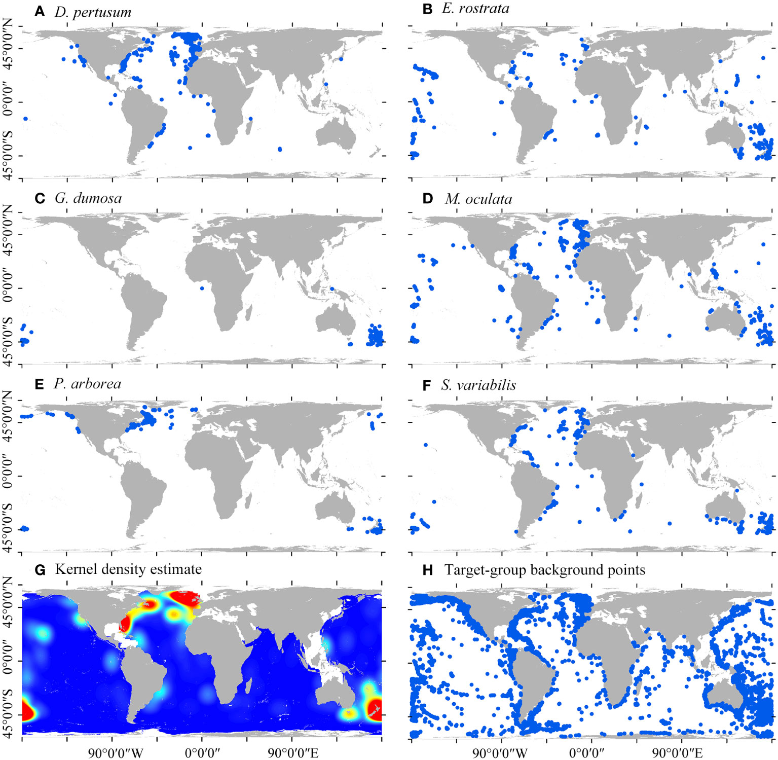
Figure 1 Global distribution of six species of cold-water corals (A–F), kernel density estimate of the six cold-water coral species (G), and the candidates of target-group background points (H).
Madrepora oculata and E. rostrata have the most widespread distributions, followed by S. varibilis, D. pertusum, and P. arborea, with G. dumosa mostly limited to the SW Pacific (Figures 1C–F). The estimated high kernel density of the six species is predominantly found in the North Atlantic and SW Pacific (Figure 1G). These global cold-water corals were particularly found on the continental shelf margin, seamounts, and deep-slope of oceanic islands (Figure 1H).
The VIFs and Pearson’s correlation of 17 environmental variables were calculated to test their correlation. A total of 12 variables were retained with VIFs < 5 and Pearson’s r < 0.8, indicating lower collinearity of the variables (Tables 2, 3). The dataset of the 12 retained environmental variables was used in predictions, and the model performances were tested and compared with the predictions using the whole dataset of environmental variables (17 variables).
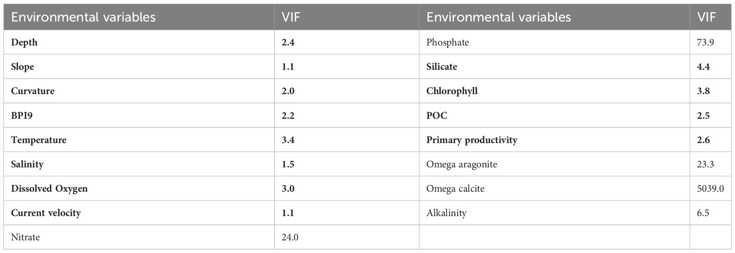
Table 2 VIFs of environmental variables, with variables and VIFs in bold in case VIF <5.
3.1 Model accuracy assessment
The response patterns of TSS are generally consistent with AUC (Figures 2A, B). All predictions performed well, with mean AUC values > 0.75. Models using kernel density backgrounds have relatively stable higher mean values of AUC and TSS statistics than corresponding models using target-group backgrounds, for all algorithms, all presence prevalence (the ratio of presences to backgrounds), and both environmental datasets (Figures 2, 3). BRT and RF have better discriminative performance than the other two algorithms, with relatively stable high mean AUC values for almost all presence prevalence and both environmental datasets (Figures 2, 3).
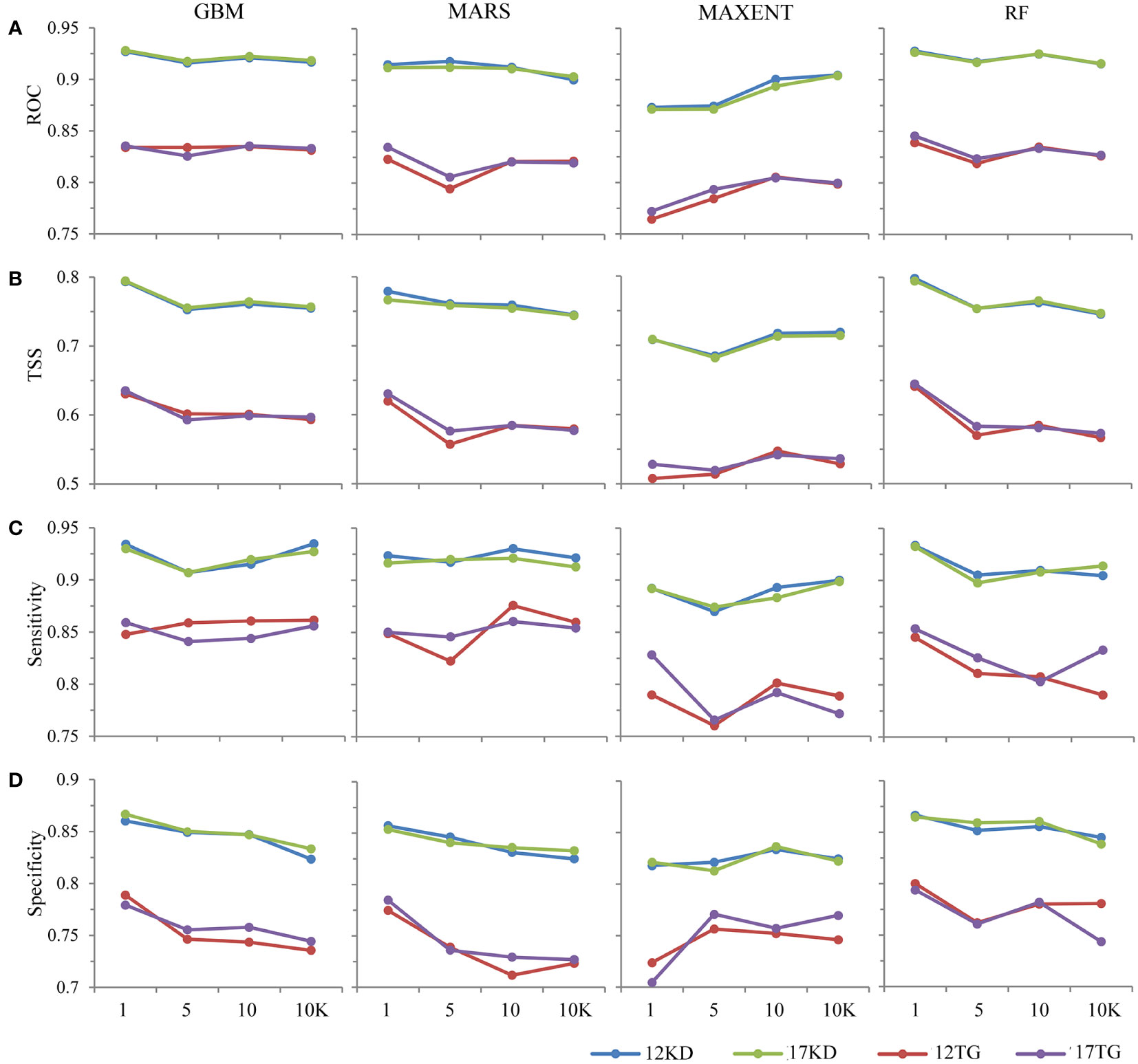
Figure 2 Discriminative performances of the predictions of the four modeling algorithms using (A) AUC, (B) TSS, (C) Sensitivity, and (D) Specificity.
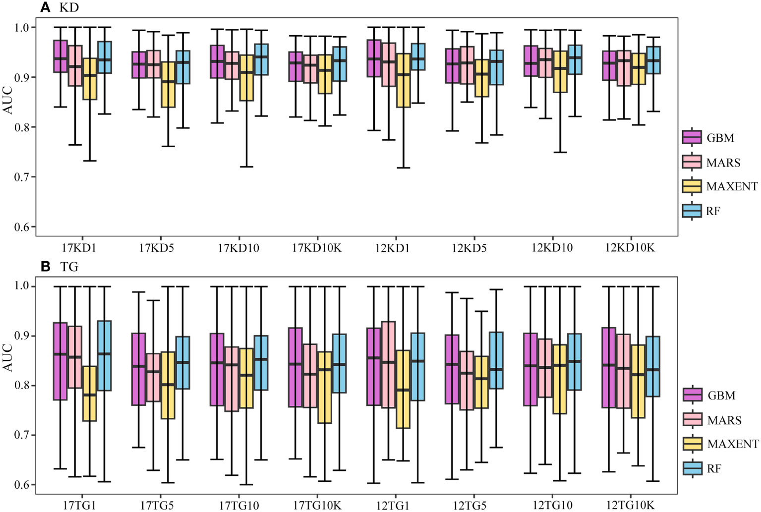
Figure 3 Boxplots of AUC values of predictions (A) using kernel density backgrounds (KD), and (B) using target-group backgrounds (TG). The x-axis label xKDy indicates predictions using x number of environmental variables, kernel density backgrounds, and a prevalence ratio or background points number y. Similarly, xTGy indicates predictions using x number of environmental variables, target-group backgrounds, and a prevalence ratio or background points number y. Here, x can be either 17 or 12, and y can be 1:1, 1:5, 1:10, or 10K. For example, 17KD1 represents predictions using 17 environmental variables, kernel density backgrounds, and a prevalence ratio 1:1, whilst 12TG10K represents predictions using 12 environmental variables, target-group backgrounds, and 10K background points.
The predictive performances of BRT, MARS, and RF using kernel density backgrounds fluctuate, with mean AUC values decreasing slightly as background prevalence decreases, whereas the mean AUC values of MAXENT increase as the prevalence decreases (Figures 2A, 3A). Models based on target-group backgrounds performed poorly compared to kernel density backgrounds, with more variability in mean AUC values (Figure 3), and lower mean discriminative performance of MAXENT than BRT, MARS, and RF, particularly for higher prevalence (Figures 2, 3).
Runs of all four algorithms are more stable using kernel density backgrounds than target-group backgrounds (Figure 3). Prediction outputs of all four algorithms are most stable for the geographically widespread M. oculata, followed by E. rostrata and D. pertusum, using kernel density backgrounds, with narrow ranges of AUC values; meanwhile, the predictions of G. dumosa consistently show the worst performance across all algorithms and backgrounds (Figure 4).

Figure 4 Boxplots of AUC values of predictions by species and background selection method. The x-axis label consists of the abbreviation of the species name and the background points sampling method. DP, D. pertusum; ER, E. rostrata; GD, G. dumosa; MO, M. oculata; PA, P. arborea; SV, S. variabilis. For example, DPKD represents predictions for D. pertusum using kernel density backgrounds, whilst SVTG represents predictions for S. variabilis using target-group backgrounds.
The mean sensitivity and specificity of predictions using kernel density backgrounds are both higher than predictions using target-group backgrounds. The mean sensitivity and specificity of RF, BRT, and MARS are mostly higher than that of MAXENT, regardless of species prevalence and environmental datasets used. Additionally, the mean sensitivity of each algorithm is higher than the corresponding specificity (Figures 2C, D).

Table 3 Pearson’s correlation matrix of 17 environmental variables, with absolute values >0.8 highlighted in bold.
3.2 Consistency assessment between modeling algorithms
Greater agreement is shown between predictions of each pair of algorithms using kernel density backgrounds than using target-group backgrounds with both environmental datasets among all four cases of species prevalence (Figure 5). Similar characteristics were found among the predictions for the six species (Figure 6). The highest agreement is evident between BRT and RF predictions using kernel density backgrounds, exhibiting a mean Pearson’s correlation coefficient ranging from 0.834 to 0.938. This is followed by BRT and MARS, with Pearson’s correlation coefficient ranging from 0.816 to 0.872, and then MARS and RF (Figure 5). In contrast, MAXENT predictions exhibit the lowest level of agreement with predictions using the other modeling techniques (Figure 5).
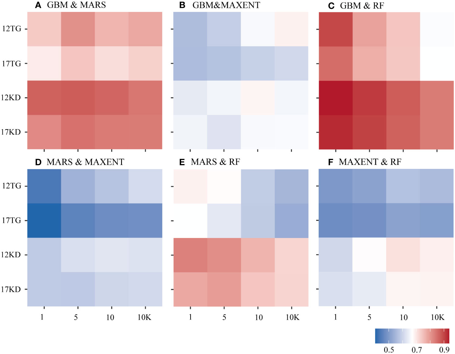
Figure 5 Pearson’s correlation coefficient was calculated between each pair of algorithms based on species prevalence. (A) GBM/BRT & MARS, (B) GBM/BRT & MAXENT, (C) GBM/BRT & RF, (D) MARS & MAXENT, (E) MARS & RF, (F) MAXENT & RF. The x-axis is labeled by prevalence ratio or background points number. Specifically, the values 1, 5, 10, and 10K represent prevalence ratios of 1:1, 1:5, and 1:10, as well as background points number of 10K. The y-axis is labeled with the number of environmental variables and the background points sampling method used. For example, 12TG represents predictions using 12 environmental variables and target-group background points, whilst 17KD represents predictions using 17 environmental variables and kernel density background points.
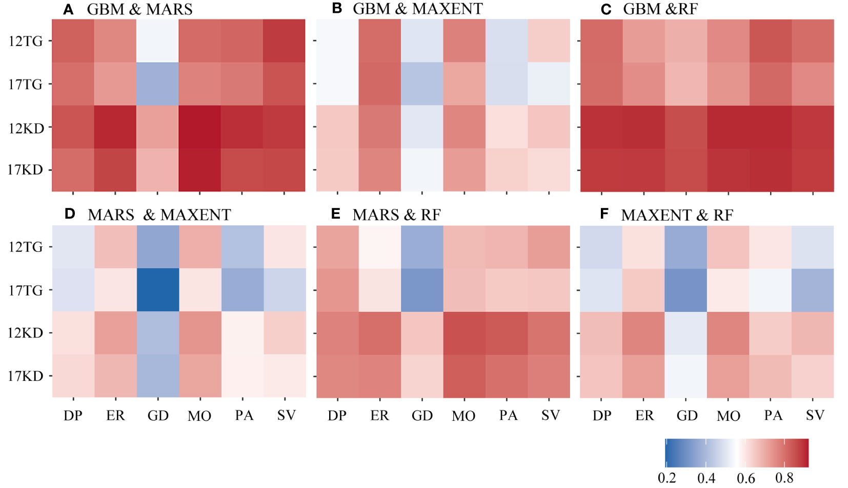
Figure 6 Pearson’s correlation coefficient was calculated between each pair of algorithms by species. (A) GBM/BRT & MARS, (B) GBM/BRT & MAXENT, (C) GBM/BRT & RF, (D) MARS & MAXENT, (E) MARS & RF and (F) MAXENT & RF. The x-axis is labeled by species name. DP, D. pertusum; ER, E. rostrata; GD, G. dumosa; MO, M. oculata; PA, P. arborea; SV, S. variabilis. The y-axis is labeled with the number of environmental variables and the background points sampling method. For example, 12TG represents predictions using 12 environmental variables and target-group background points, whilst 17KD represents predictions using 17 environmental variables and kernel density background points.
The greatest mean agreement between BRT and RF was observed in predictions using a prevalence ratio of 1:1 and the filtered environmental dataset (12 environmental variables), yielding a Pearson’s correlation coefficient of 0.938. This is followed by predictions using a prevalence ratio of 1:1 and the whole environmental dataset (17 variables), resulting in a Pearson’s correlation coefficient of 0.925. The level of agreement decreases as prevalence decreases (Figure 5).
When using kernel density backgrounds, the mean agreement between BRT and RF predictions ranks among the top for five out of six species, except for G. dumosa. Madrepora oculata and E. rostrata show the highest mean agreement in predictions for each pair of algorithms, while the least agreement is found in G. dumosa predictions for each pair of algorithms (Figure 6).
3.3 Consistency assessment of each modeling algorithm
Fleiss’ kappa statistics highlight a stronger mean agreement of predictions for each algorithm when using kernel density backgrounds compared to target-group backgrounds. The mean Fleiss’ kappa ranges between 0.46 and 0.641 in predictions using kernel density backgrounds (Figure 7).
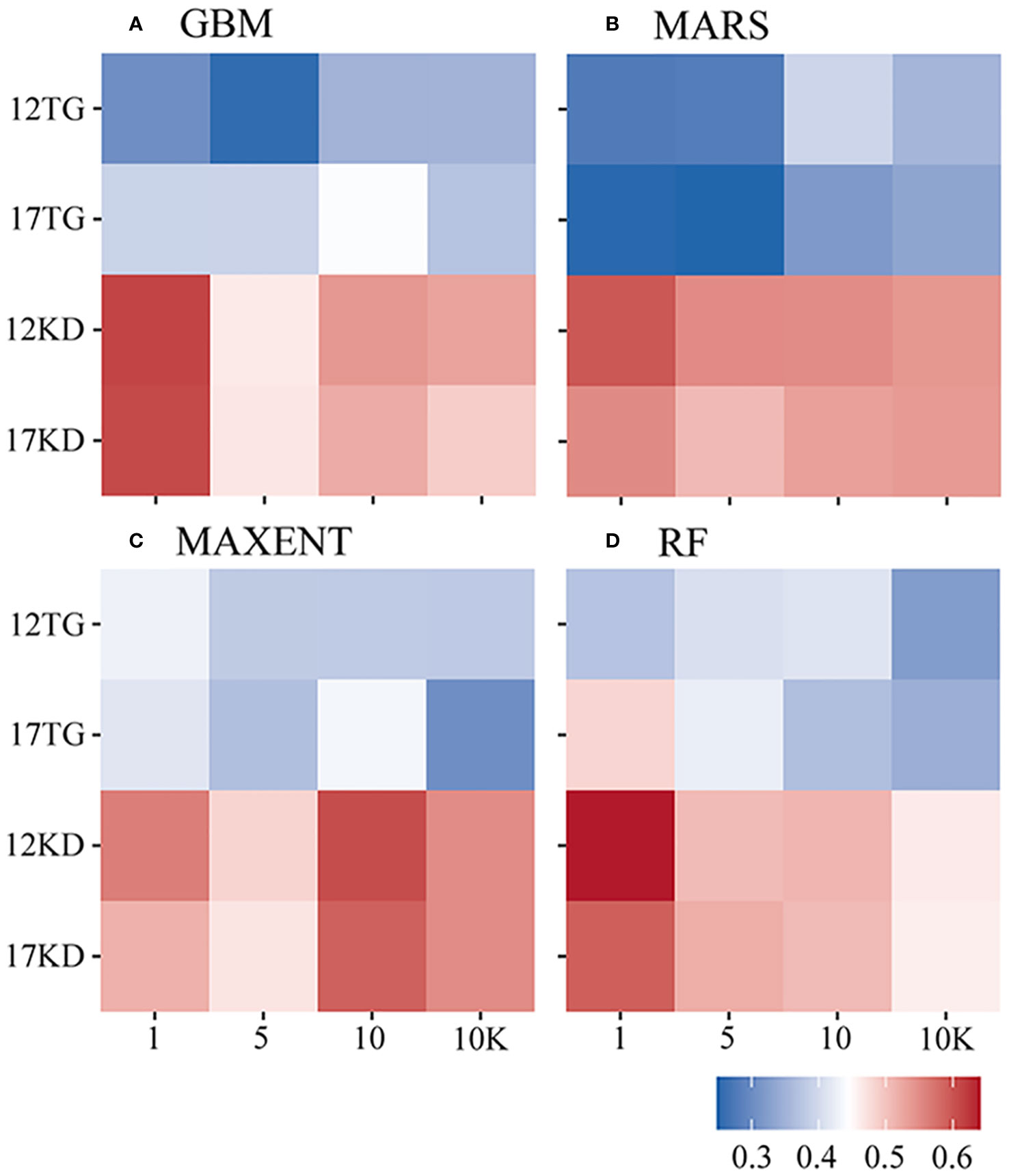
Figure 7 Fleiss’ kappa statistic of each algorithm by species prevalence. (A) GBM/BRT, (B) MARS, (C) MAXENT, and (D) RF. The x-axis is labeled by prevalence ratio or background points number. Specifically, the values 1, 5, 10, and 10K represent prevalence ratios of 1:1, 1:5, and 1:10, as well as background points number of 10K. The y-axis is labeled with the number of environmental variables and the background points sampling method used. For example, 12TG represents predictions using 12 environmental variables and target-group background points, whilst 17KD represents predictions using 17 environmental variables and kernel density background points.
The strongest agreement of predictions for each algorithm is achieved in cases where the filtered environmental dataset is used, and an equal number of background points to presences is used (prevalence 1:1) for BRT, MARS, and RF predictions. For MAXENT predictions, a prevalence ratio of 1:10 is employed. The highest mean Fliess’ kappa values are recorded for RF (0.641, 12KD1), followed by BRT (0.613, 12KD1), MARS (0.596, 12KD1), and MAXENT (0.606, 12KD10) (Figure 7).
The lowest agreement for each algorithm is observed in predictions of G. dumosa, using both kernel density backgrounds and target-group backgrounds, as well as both environmental datasets. For M. oculata, high Fleiss’ kappa values are noted in BRT, MARS, and RF predictions, particularly when using the filtered environmental dataset (12KDMO), with corresponding values of 0.729, 0.756, and 0.689, respectively. Conversely, the Fleiss’ kappa value for E. rostrata is high in MAXENT prediction, particularly when using the filtered environmental dataset (12KDER) at 0.685. Notably, high agreement for each algorithm is also observed in predictions for S. varibilis using target-group backgrounds (Figure 8).

Figure 8 Fleiss’ kappa statistic of each algorithm by species. (A) GBM/BRT, (B) MARS, (C) MAXENT, and (D) RF. The x-axis is labeled by species name. DP, D. pertusum; ER, E. rostrata; GD, G. dumosa; MO, M. oculata; PA, P. arborea; SV, S. variabilis. The y-axis is labeled with the number of environmental variables and the background points sampling method used. For example, 12TG represents predictions using 12 environmental variables and target-group background points, whilst 17KD represents predictions using 17 environmental variables and kernel density background points.
3.4 Spatial residuals and uncertainty of predicted habitat suitability for M. oculata
Figure 9; Supplementary Figure 1 illustrate that the spatial residuals of RF predictions are lower compared to predictions of BRT, MARS, and MAXENT. When using a 1:1 ratio of presence to backgrounds, BRT predictions exhibit fewer areas of high residuals compared to using backgrounds of 1:5, 1:10, and 10K. A similar trend is observed in MARS predictions. However, in the case of MAXENT predictions, using a 1:1 ratio of presence to pseudo-absence leads to more areas of high residuals compared to backgrounds of 1:5, 1:10, and 10K.
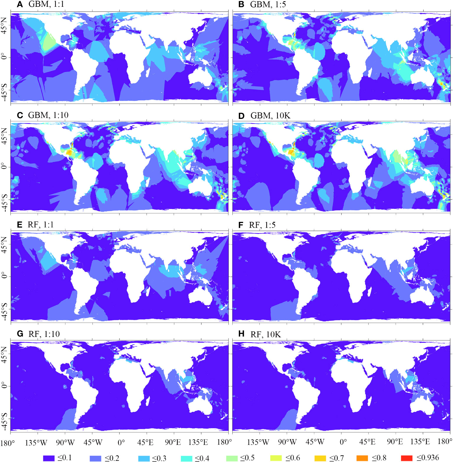
Figure 9 Smoothed residuals of predicted habitat suitability for M. oculata, utilizing GBM/BRT and RF models. Prevalence ratios of 1:1, 1:5, and 1:10, as well as background points number of 10K, and 12 environmental variables selected using VIF were employed. (A) GBM, 1:1; (B) GBM, 1:5; (C) GBM, 1:10; (D) GBM, 10K; (E) RF, 1:1; (F) RF, 1:5; (G) RF, 1:10; (H) RF, 10K.
Figure 10; Supplementary Figure 2 illustrate that the uncertainty of BRT and RF predictions is lower compared to MARS and MAXENT predictions. Among them, MAXENT predictions display the highest level of uncertainty, with the 1:10 ratio prediction showing fewer areas of high uncertainty compared to other ratio cases.
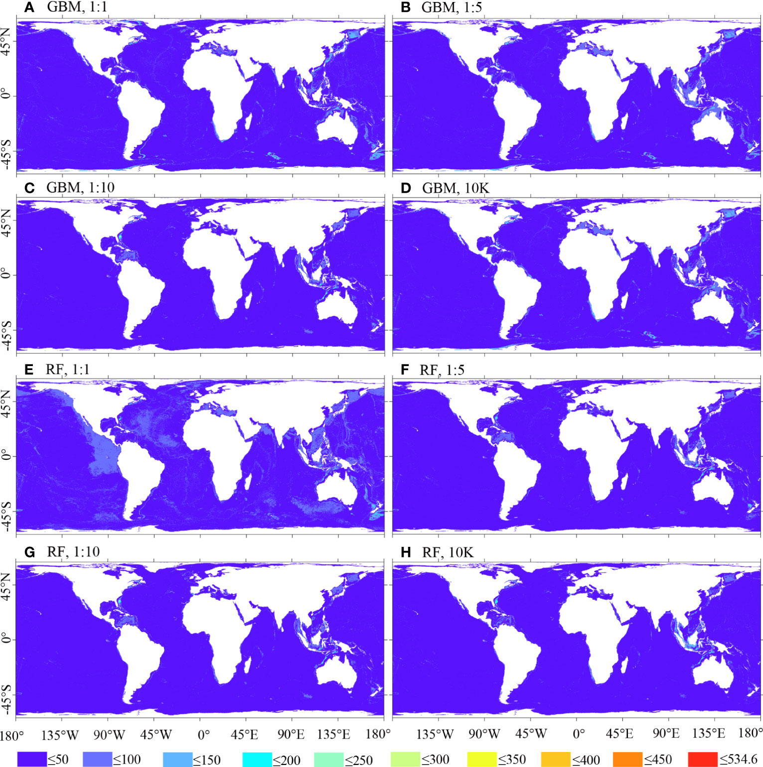
Figure 10 Uncertainty of predicted habitat suitability for M. oculata, utilizing GBM/BRT and RF models. Prevalence ratios of 1:1, 1:5, and 1:10, as well as background points number of 10K, and 12 environmental variables selected using VIF were employed.(A) GBM, 1:1; (B) GBM, 1:5; (C) GBM, 1:10; (D) GBM, 10K; (E) RF, 1:1; (F) RF, 1:5; (G) RF, 1:10; (H) RF, 10K.
Supplementary Figure 3 provides visual assessments of the predicted habitat suitability maps for M. oculata. It reveals a similar spatial pattern among the predicted habitat suitability of the four modeling algorithms, with high habitat suitability generally aligning with the spatial locations of M. oculata presences.
4 Discussion
In this study, alongside discriminative accuracy measuring metrics (AUC, TSS, sensitivity, and specificity), functional performance measuring metrics (Fleiss’ kappa, Pearson’s correlation coefficient smoothed spatial residuals and standard deviation) were employed to explore the influence of four key factors on species distribution modeling, including sampling strategies and number of background points, collinearity of environmental variables, and modeling algorithms. This investigation was carried out using the global distribution predictions of six real cold-water coral species as a case study.
4.1 Impact of sampling strategy of background points on predictive performance
The study revealed a pronounced spatial bias in species presence records, with the highest sampling intensity concentrated in the North Atlantic and SW Pacific regions (Figure 1). Spatial sampling biases in biodiversity data emerge from intricate interactions among geography, species traits, and human behavior (e.g., preferences or avoidance of certain species or habitats) (Baker et al., 2022). Addressing this sampling bias poses a significant challenge for presence-only and presence-background species distribution models. Biased data can obscure the actual correlation between occurrences and environmental predictors, irrespective of the model used, leading to predictive distributions that predominantly reflect sampling effort rather than actual habitat suitability (Baker et al., 2022; Barber et al., 2022). In this study, the sampling strategy of background points was identified as the most influential factor on predictive performance, surpassing the effects of modeling algorithms, species prevalence (the ratio of species presences to background points), or collinearity of environmental datasets (Figure 2).
Kernel density background data demonstrated significantly superior performance compared to target-group backgrounds in achieving higher discriminative accuracy and functional performance across all four algorithms, all species prevalence cases, both environmental datasets, and different niche breadths (Figures 2, 7, 8). Although direct performance accuracy comparisons between predictions using kernel density backgrounds and target-group backgrounds have been sparse in previous studies, these methods have been favorably compared to other techniques aimed at reducing sampling bias. Target-group backgrounds outperformed radius-restricted backgrounds and covariates of sampling effort (e.g., maps of human population density and road networks) used as alternative means to estimate sampling effort, effectively mitigating the impact of sampling bias (Barber et al., 2022). Moreover, modeling with target-group backgrounds exhibited superior performance compared to random backgrounds (Phillips et al., 2009) and environmental-filtering backgrounds (Iturbide et al., 2015). Modeling using kernel density backgrounds exhibited a greater improvement in recreating known distributions compared to presences-filtering methods, which encompass spatially thinning presences to a fixed sampling density using geographic filtering or maintaining equal sampling intensity across environmental space using environmental filtering (Inman et al., 2021).
We speculate that the comparable distribution pattern of the six species with target-group backgrounds, often found on the continental shelf margin, seamounts, and steep slopes of sea islands (Figure 1), could heighten the probability that background points (cells) indeed contain species occurrences. This increased likelihood could lead to greater difficulty in distinguishing between presences and backgrounds, ultimately diminishing the predictive performance of models using target-group backgrounds.
4.2 Impact of number of background points on predictive performance
The study revealed that different algorithms performed optimally with distinct background sampling sizes, a relationship also observed in previous studies (Barbet-Massin et al., 2012; Liu et al., 2019). The findings regarding machine learning methods BRT and RF are consistent with previous research. Grimmett et al. (2020); Barbet-Massin et al. (2012); Jimenex-Valverde (2021); Hysen et al. (2022), and Barker & MacIsaac (2022) all support an equal prevalence of presences and absences. Liu et al. suggested a small multiplier in background points relative to the number of presences (Barbet-Massin et al., 2012; Liu et al., 2019; Grimmett et al., 2020; Jimenez-Valverde, 2021; Barker and MacIsaac, 2022; Hysen et al., 2022).
The conclusions regarding the optimal size of background samples for the MARS algorithm have been conflicting in previous studies. Hysen et al. (2022) found that MARS performed optimally with 10,000 background points for a sample size of 248 (Hysen et al., 2022), while Barbet-Massin et al. (2012) suggested fewer pseudo-absences (e.g., 100) for sample sizes of 30, 100, 300, or 1000 presences. However, our findings align with Barker and MacIsaac (2022), who recommended equal random pseudo-absences to centroids (presences). The reduced areas of high residuals in the predicted habitat suitability of MARS using a 1:1 ratio of presence to backgrounds, compared to other background ratios (Supplementary Figures 1, 2), also signify the higher accuracy of predictions using a 1:1 ratio.
Likewise, conclusions regarding the optimal size of background samples for the MAXENT algorithm have been conflicting in previous studies. Liu et al. (2019) found that MAXENT performed optimally using background points as a small multiple of presences, and Barker and MacIsaac (2022) suggested equal random pseudo-absences to centroids (presences). However, our findings align with Grimmett et al. (2020) (e.g., 1900 background points for 100 presences), Phillips and Dudík (2008) (e.g., 10,000 for a few to thousands of presences) (Phillips and Dudík, 2008), and Hysen et al. (2022) (prevalence 1:10 is better than prevalence 1:1 and 10,000 sample size). The reduced areas of high residuals and lower uncertainty in the predicted habitat suitability of MAXENT using a 1:10 ratio of presence to backgrounds, compared to other background ratios, also indicate the higher accuracy of predictions using a 1:10 ratio.
Concerning prediction consistency, our results correspond with Grimmett et al. (2020), who identified the strongest agreement (Fleiss’ kappa statistic) between RF predictions using equal presence backgrounds and between MAXENT predictions using a large number of background points. Moreover, our results align with other studies that advocate equal presence-backgrounds in BRT, RF, and MARS predictions, while recommending the use of a substantial number of background points for MAXENT predictions.
4.3 Impact of modeling algorithms on predictive performance
No single modeling algorithm outperformed all others under all circumstances. Nonetheless, in this study, BRT & RF performed best overall using equal prevalence. However, MAXENT and BRT exhibited better performance than RF in predictions involving 225 species with dozens to thousands of presences (Elith et al., 2006; Valavi et al., 2021). Similarly, MAXENT outperformed other algorithms, such as a variant of RF, BRT, and MARS, in predictions involving 171 species in both random and spatial partitioning (Valavi et al., 2023). However, a number of previous studies have reported different outcomes, which are consistent with our results. For instance, Barker and MacIsaac (2022) found BRT to outperform RF, MARS, and MAXENT in predictions involving virtual species; Romero-Sanchez et al. (2022) found RF to achieve better performance than MAXENT in predictions for plus trees; and Hysen et al. (2022) found RF to perform better than MARS and MAXENT in nest predictions (Barker and MacIsaac, 2022; Hysen et al., 2022; Romero-Sanchez et al., 2022). Additionally, the smaller number of areas with high residuals and lower uncertainty in the predicted habitat suitability of RF and BRT, compared to those of MARS and MAXENT in M. oculata prediction, also indicates the higher accuracy of predictions using RF and BRT.
Our finding that the greatest agreement of MAXENT showed lower than BRT or RF is in conflict with the result of Grimmett et al. (2020), which found that MAXENT performed more consistently in terms of discriminative accuracy and spatial prediction stability than RF using 20 to 100 presences, and a background sample size determined by presences/(presences + background points) = 0.5, 0.1, 0.05, 0.01, and 0.005 (Grimmett et al., 2020). Additionally, Grimmett et al. (2020) found that Pearson’s correlation coefficient between RF and MAXENT increased with prevalence (~0.3-0.9). The inconsistent result from our study could be related to different sample sizes (20-100 presences in their study, 316-1223 presences in this study) and validation metrics between studies (random cross-validation in their study and spatial block cross-validation in this study). In general, increasing sample size has a positive effect on performance (measured by AUC and Schoener´s D), with model accuracy decreasing with a sample size below 300 presences (Gábor et al., 2020). Both Fleiss’ kappa of MAXENT and RF predictions increased with increasing sample size in Grimmett et al. (2020), which may indicate that the conflicting results may be related to differences in sample size.
4.4 Impact of collinearity of environmental variables on predictive performance
The AUC values were found to be similar between predictions using the 12 filtered (uncorrelated) environmental variables and the full set of 17 correlated variables for each of the four modeling techniques, particularly when using kernel density backgrounds, indicating that the collinearity of the environmental dataset did not influence the discriminative accuracy of the four modeling methods significantly. Dormann et al. (2013) also found that the modeling methods significantly, GAM, MARS, BRT, and RF, worked reasonably well under moderate collinearity (Dormann et al., 2013). de Marco Junior and Nobrega (2018) found that the intensity of the effect of collinearity varied according to the algorithm characteristics, with more complex models, such as MAXENT, performing better than simple envelope ones based on PCA-derived variables (de Marco Junior and Nobrega, 2018). However, the collinearity of the environmental dataset did influence the functional performance of algorithms, with stronger agreement of each algorithm found in predictions using the VIF-filtered environmental dataset compared to when using the whole dataset. Furthermore, spatial autocorrelation in the predictors can inflate the variable importance estimates when the response of species to the environmental gradients is linear (Harisena et al., 2021). Therefore, it is recommended to address the collinearity between environmental variables before modeling.
It is worth noting that the methodologies employed in our study, namely, the use of different modeling algorithms, background sampling strategies, number of background points, and collinearity of environmental variables, are not exclusive to the study of cold-water corals, although specific cold-water coral species within the Hexocorallia and Octocorellia groups were used as a case study. These approaches can be widely applicable in species distribution modeling across various marine benthic taxa. Therefore, the insights gained from our investigation into the impact of these factors on predictive performance could potentially extend to other benthic groups and marine species. However, different species with different habitat preferences, ecological requirements, and dispersal abilities may exhibit unique responses to these factors. Therefore, while the specific results of our study pertain to cold-water corals, the underlying principles and considerations can serve as a foundation for researchers working with other marine species.
5 Conclusion
We found that all four algorithms tested performed well for both kernel density backgrounds and target-group backgrounds, all presence prevalence, and both environmental datasets, particularly BRT and RF. However, the choice of background sampling method was found to have a stronger influence on model performance than modeling algorithms, presence prevalence, or collinearity of environmental datasets. We recommend using kernel density backgrounds; an equal number of presences and background points for algorithms of BRT, RF, and MARS; and a large number of background points for MAXENT, such as 10 times the presences or 10K, using a collinearity filtered environmental dataset in species distribution modeling for higher discriminative and functional performance.
Data availability statement
The raw data supporting the conclusions of this article will be made available by the authors, without undue reservation.
Author contributions
RT and CY contributed to the conception and design of the study. RT, JY, YL, and LZ preprocessed the data, created the codes, performed the modeling, and provided the statistical analysis. The manuscript was written by RT and was contributed to and edited by CY. All authors contributed to the article and approved the submitted version.
Funding
This research is supported by the National Natural Science Foundation of China (NO. 42006140), the National Key R&D Program of China (NO. 2019. YFE0127100), and the Natural Science Foundation of Fujian Province of China (No.2019I0006). ZSL Institute of Zoology staff are financially supported by Research England.
Conflict of interest
The authors declare that the research was conducted in the absence of any commercial or financial relationships that could be construed as a potential conflict of interest.
Publisher’s note
All claims expressed in this article are solely those of the authors and do not necessarily represent those of their affiliated organizations, or those of the publisher, the editors and the reviewers. Any product that may be evaluated in this article, or claim that may be made by its manufacturer, is not guaranteed or endorsed by the publisher.
Supplementary material
The Supplementary Material for this article can be found online at: https://www.frontiersin.org/articles/10.3389/fmars.2023.1222382/full#supplementary-material
References
Allouche O., Tsoar A., Kadmon R. (2006). Assessing the accuracy of species distribution models: prevalence, kappa and the true skill statistic (TSS). J. Appl. Ecol. 43, 1223–1232. doi: 10.1111/j.1365-2664.2006.01214.x
Anderson O. F., Stephenson F., Behrens E., Rowden A. A. (2022). Predicting the effects of climate change on deep-water coral distribution around New Zealand-Will there be suitable refuges for protection at the end of the 21st century? Global Change Biol. 28, 6556–6576. doi: 10.1111/gcb.16389
Assis J., Tyberghein L., Bosch S., Verbruggen H., Serrao E. A., De Clerck O. (2018). Bio-ORACLE v2.0: Extending marine data layers for bioclimatic modelling. Global Ecol. Biogeography 27, 277–284. doi: 10.1111/geb.12693
Baker D. J., Maclean I. M. D., Goodall M., Gaston K. J. (2022). Correlations between spatial sampling biases and environmental niches affect species distribution models. Global Ecol. Biogeography 31, 1038–1050. doi: 10.1111/geb.13491
Barber R. A., Ball S. G., Morris R. K. A., Gilbert F. (2022). Target-group backgrounds prove effective at correcting sampling bias in Maxent models. Diversity Distributions 28, 128–141. doi: 10.1111/ddi.13442
Barbet-Massin M., Jiguet F., Albert C. H., Thuiller W. (2012). Selecting pseudo-absences for species distribution models: how, where and how many? Methods Ecol. Evol. 3, 327–338. doi: 10.1111/j.2041-210X.2011.00172.x
Barbosa R. V., Davies A. J., Sumida P. Y. G. (2020). Habitat suitability and environmental niche comparison of cold-water coral species along the Brazilian continental margin. Deep-Sea Res. Part I, 155. doi: 10.1016/j.dsr.2019.103147
Barker J. R., MacIsaac H. J. (2022). Species distribution models: Administrative boundary centroid occurrences require careful interpretation. Ecol. Model. 472. doi: 10.1016/j.ecolmodel.2022.110107
Basher Z., Bowden D. A., Costello M. J. (2018). Global Marine Environment Datasets (GMED). World Wide Web electronic Publ. http://gmed.auckland.ac.nz.
Buhl-Mortensen L., Vanreusel A., Gooday A., Levin L., Priede I., Buhl-Mortensen P., et al. (2010). Biological structures as a source of habitat heterogeneity and biodiversity on the deep ocean margins. Mar. Ecol. 31, 21–50. doi: 10.1111/j.1439-0485.2010.00359.x
Burgos J. M., Buhl-Mortensen L., Buhl-Mortensen P., Olafsdottir S. H., Steingrund P., Ragnarsson S. A., et al. (2020). Predicting the distribution of indicator taxa of vulnerable marine ecosystems in the arctic and sub-arctic waters of the nordic seas. Front. Mar. Sci. 7. doi: 10.3389/fmars.2020.00131
Cerasoli F., Iannella M., D’Alessandro P., Biondi M. (2017). Comparing pseudo-absences generation techniques in Boosted Regression Trees models for conservation purposes: A case study on amphibians in a protected area. PloS One 12, e0187589. doi: 10.1371/journal.pone.0187589
Davies A. J., Guinotte J. M. (2011). Global habitat suitability for framework-forming cold-water corals. PloS One 6. doi: 10.1371/journal.pone.0018483
de Froe E., Rovelli L., Glud R. N., Maier S. R., Duineveld G., Mienis F., et al. (2019). Benthic oxygen and nitrogen exchange on a cold-water coral reef in the north-east atlantic ocean. Front. Mar. Sci. 6. doi: 10.3389/fmars.2019.00665
DeLong E. R., DeLong D. M., Clarke-Pearson D. L. (1988). Comparing the areas under two or more correlated receiver operating characteristic curves: A nonparametric approach. Biometrics 44, 837–845. doi: 10.2307/2531595
de Marco Junior P., Nobrega C. C. (2018). Evaluating collinearity effects on species distribution models: An approach based on virtual species simulation. PloS One 13. doi: 10.1371/journal.pone.0202403
Di Cola V., Broennimann O., Petitpierre B., Breiner F. T., D’Amen M., Randin C., et al. (2017). ecospat: an R package to support spatial analyses and modeling of species niches and distributions. Ecography 40, 774–787. doi: 10.1111/ecog.02671
Dormann C. F., Elith J., Bacher S., Buchmann C., Carl G., Carre G., et al. (2013). Collinearity: a review of methods to deal with it and a simulation study evaluating their performance. Ecography 36, 27–46. doi: 10.1111/j.1600-0587.2012.07348.x
Elith J., Graham C. H., Anderson R. P., Dudı´ K. ,. M., Ferrier S., Guisan A., et al. (2006). Novel methods improve prediction of species’ distributions from occurrence data. Ecography 29, 129–151. doi: 10.1111/j.2006.0906-7590.04596.x
Elith J., Kearney M., Phillips S. (2010). The art of modelling range-shifting species. Methods Ecol. Evol. 1, 330–342. doi: 10.1111/j.2041-210X.2010.00036.x
Elith J., Phillips S. J., Hastie T., Dudík M., Chee Y. E., Yates C. J. (2011). A statistical explanation of MaxEnt for ecologists. Diversity Distributions 17, 43–57. doi: 10.1111/j.1472-4642.2010.00725.x
Finucci B., Duffy C. A., Brough T., Francis M. P., Milardi M., Pinkerton M. H., et al. (2021). Drivers of spatial distributions of basking shark (Cetorhinus maximus) in the Southwest Pacific. Front. Mar. Sci. 8. doi: 10.3389/fmars.2021.665337
Fitzpatrick M. C., Gotelli N. J., Ellison A. M. (2013). MaxEnt versus MaxLike: empirical comparisons with ant species distributions. Ecosphere 4, 1–15. doi: 10.1890/ES13-00066.1
Fleiss J. L. (1971). Measuring nominal scale agreement among many raters. psychol. Bull. 76, 378–382. doi: 10.1037/h0031619
Freeman E. A., Moisen G. G., Coulston J. W., Wilson B. T. (2016). Random forests and stochastic gradient boosting for predicting tree canopy cover: comparing tuning processes and model performance. Can. J. For. Res. 46, 323–339. doi: 10.1139/cjfr-2014-0562
Friedman J. H. (1991). Multivariate adaptive regression splines. Ann. Of Stat 19, 1–67. doi: 10.1214/aos/1176347963
Friedman J. H. (2001). Greedy function approximation: A gradient boosting machine. Ann. Stat 29, 1189–1232. doi: 10.1214/aos/1013203451
Gábor L., Moudrý V., Barták V., Lecours V. (2020). How do species and data characteristics affect species distribution models and when to use environmental filtering? Int. J. Geographical Inf. Sci. 34, 1567–1584. doi: 10.1080/13658816.2019.1615070
Georgian S. E., Anderson O. F., Rowden A. A. (2019). Ensemble habitat suitability modeling of vulnerable marine ecosystem indicator taxa to inform deep-sea fisheries management in the South Pacific Ocean. Fisheries Res. 211, 256–274. doi: 10.1016/j.fishres.2018.11.020
Georgian S., Morgan L., Wagner D. (2021). The modeled distribution of corals and sponges surrounding the Salas y Gomez and Nazca ridges with implications for high seas conservation. PeerJ 9. doi: 10.7717/peerj.11972
Gonzalez-Mirelis G., Ross R. E., Albretsen J., Buhl-Mortensen P. (2021). Modeling the distribution of habitat-forming, deep-sea sponges in the barents sea: the value of data. Front. Mar. Sci. 7. doi: 10.3389/fmars.2020.496688
Grimmett L., Whitsed R., Horta A. (2020). Presence-only species distribution models are sensitive to sample prevalence: Evaluating models using spatial prediction stability and accuracy metrics. Ecol. Model. 431. doi: 10.1016/j.ecolmodel.2020.109194
Harisena N. V., Groen T. A., Toxopeus A. G., Naimi B. (2021). When is variable importance estimation in species distribution modelling affected by spatial correlation? Ecography 44, 778–788. doi: 10.1111/ecog.05534
Heiberger R. M. (2022). HH: Statistical Analysis and Data Display: Heiberger and Holland. R package version 31-49. Available at: https://CRANR-projectorg/package=HH.
Heiberger R. M., Holland B. (2004). Statistical Analysis and Data Display An Intermediate Course with Examples in S-Plus, R, and SAS (Springer).
Hu W., Du J., Su S., Tan H., Yang W., Ding L., et al. (2022). Effects of climate change in the seas of China: Predicted changes in the distribution of fish species and diversity. Ecol. Indic. 134. doi: 10.1016/j.ecolind.2021.108489
Hysen L., Nayeri D., Cushman S., Wan H. Y. (2022). Background sampling for multi-scale ensemble habitat selection modeling: Does the number of points matter? Ecol. Inf. 72. doi: 10.1016/j.ecoinf.2022.101914
Inman R., Franklin J., Esque T., Nussear K. (2021). Comparing sample bias correction methods for species distribution modeling using virtual species. Ecosphere 12. doi: 10.1002/ecs2.3422
Iturbide M., Bedia J., Herrera S., Hierro O. D., Pinto M., Gutiérrez J. M. (2015). A framework for species distribution modelling with improved pseudo-absence generation. Ecol. Model. 312, 166–174. doi: 10.1016/j.ecolmodel.2015.05.018
Jaynes E. T. (1957). Information theory and statistical mechanics. Phys. Rev. 106, 620–630. doi: 10.1103/PhysRev.106.620
Jiménez-Valverde A. (2012). Insights into the area under the receiver operating characteristic curve (AUC) as a discrimination measure in species distribution modelling. Global Ecol. Biogeography 21, 498–507. doi: 10.1111/j.1466-8238.2011.00683.x
Jimenez-Valverde A. (2021). Prevalence affects the evaluation of discrimination capacity in presence-absence species distribution models. Biodiversity Conserv. 30, 1331–1340. doi: 10.1007/s10531-021-02144-4
Jorcin P., Barthe L., Berroneau M., Dore F., Geniez P., Grillet P., et al. (2019). Modelling the distribution of the Ocellated Lizard in France: implications for conservation. Amphibian Reptile Conserv. 13, 276–298.
Khosravifard S., Skidmore A. K., Toxopeus A. G., Niamir A. (2020). Potential invasion range of raccoon in Iran under climate change. Eur. J. Wildlife Res. 66. doi: 10.1007/s10344-020-01438-2
Lee C. M., Lee D. S., Kwon T. S., Athar M., Park Y. S. (2021). Predicting the Global Distribution of Solenopsis geminata (Hymenoptera: Formicidae) under Climate Change Using the MaxEnt Model. Insects 12. doi: 10.3390/insects12030229
Liu C., Newell G., White M. (2015). On the selection of thresholds for predicting species occurrence with presence-only data. Ecol. Evol. 6, 337–348. doi: 10.1002/ece3.1878
Liu C. R., Newell G., White M. (2019). The effect of sample size on the accuracy of species distribution models: considering both presences and pseudo-absences or background sites. Ecography 42, 535–548. doi: 10.1111/ecog.03188
Liu C. R., White M., Newell G. (2013). Selecting thresholds for the prediction of species occurrence with presence-only data. J. Biogeography 40, 778–789. doi: 10.1111/jbi.12058
Lobo J. M., Jiménez-Valverde A., Hortal J. (2010). The uncertain nature of absences and their importance in species distribution modelling. Ecography 33, 103–114. doi: 10.1111/j.1600-0587.2009.06039.x
Lobo J. M., Tognelli M. F. (2011). Exploring the effects of quantity and location of pseudo-absences and sampling biases on the performance of distribution models with limited point occurrence data. J. Nat. Conserv. 19, 1–7. doi: 10.1016/j.jnc.2010.03.002
Locarnini R. A., Mishonov A. V., Baranova O. K., Boyer T. P., Zweng M. M., Garcia H. E., et al. (2018). World ocean atlas 2018, volume 1: temperature (Mishonov A., Technical Editor). NOAA Atlas NESDIS 81, Silver Spring.
Lutz M., Caldeira K., Dunbar R., Behrenfeld M. (2007). Seasonal rhythms of net primary production and particulate organic carbon flux to depth describe the efficiency of biological pump in the global ocean. J. Geophysical Res. 112, C10011. doi: 10.1029/2006JC003706
Matos F. L., Company J. B., Cunha M. R. (2021). Mediterranean seascape suitability for Lophelia pertusa: Living on the edge. Deep-Sea Res. Part I-Oceanographic Res. Papers 170. doi: 10.1016/j.dsr.2021.103496
Merow C., Allen J. M., Aiello-Lammens M., Silander J. A. Jr. (2016). Improving niche and range estimates with Maxent and point process models by integrating spatially explicit information. Global Ecol. Biogeography 25, 1022–1036. doi: 10.1111/geb.12453
Merow C., Smith M. J., Silander J. A. (2013). A practical guide to MaxEnt for modeling species’ distributions: what it does, and why inputs and settings matter. Ecography 36, 1058–1069. doi: 10.1111/j.1600-0587.2013.07872.x
Morato T., Gonzalez-Irusta J.-M., Dominguez-Carrio C., Wei C.-L., Davies A., Sweetman A. K., et al. (2020). Climate-induced changes in the suitable habitat of cold-water corals and commercially important deep-sea fishes in the North Atlantic. Global Change Biol. 26. doi: 10.1111/gcb.14996
Phillips S. J., Anderson R. P., Schapire R. E. (2006). Maximum entropy modeling of species geographic distributions. Ecol. Model. 190, 231–259. doi: 10.1016/j.ecolmodel.2005.03.026
Phillips S. J., Dudík M. (2008). Modeling of species distributions with Maxent: new extensions and a comprehensive evaluation. Ecography 31, 161–175. doi: 10.1111/j.0906-7590.2008.5203.x
Phillips S. J., Dudik M., Elith J., Graham C. H., Lehmann A., Leathwick J., et al. (2009). Sample selection bias and presence-only distribution models: implications for background and pseudo-absence data. Ecol. Appl. 19, 181–197. doi: 10.1890/07-2153.1
Principe S. C., Acosta A. L., Andrade J. E., Lotufo T. M. C. (2021). Predicted shifts in the distributions of atlantic reef-building corals in the face of climate change. Front. Mar. Sci. 8. doi: 10.3389/fmars.2021.673086
Ramirez-Llodra E., Brandt A., Danovaro R., De Mol B., Escobar E., German C. R., et al. (2010). Deep, diverse and definitely different: unique attributes of the world’s largest ecosystem. Biogeosciences 7, 2851–2899. doi: 10.5194/bg-7-2851-2010
Renner I. W., Elith J., Baddeley A., Fithian W., Hastie T., Phillips S. J., et al. (2015). Point process models for presence-only analysis. Methods Ecol. Evol. 6, 366–379. doi: 10.1111/2041-210x.12352
Roberts J., Wheeler A., Freiwald A. (2006). Reefs of the deep: the biology and geology of cold-water coral ecosystems. Science 312, 543–547. doi: 10.1126/science.1119861
Robinson C. L. K., Proudfoot B., Rooper C. N., Bertram D. F. (2021). Comparison of spatial distribution models to predict subtidal burying habitat of the forage fish Ammodytes personatus in the Strait of Georgia, British Columbia, Canada. Aquat. Conservation-Marine Freshw. Ecosyst. 31, 2855–2869. doi: 10.1002/aqc.3593
Romero-Sanchez M. E., Velasco-Garcia M. V., Perez-Miranda R., Velasco-Bautista E., Gonzalez-Hernandez A. (2022). Different modelling approaches to determine suitable areas for conserving egg-cone pine (Pinus oocarpa schiede) plus trees in the central part of Mexico. Forests 13. doi: 10.3390/f13122112
Rowden A., Stephenson F., Clark M., Anderson O., Guinotte J., Baird S., et al (2019). Examining the utility of a decision-support tool to develop spatial management options for the protection of vulnerable marine ecosystems on the high seas around New Zealand. Ocean Coast. Manage. 170, 1–16. doi: 10.1016/j.ocecoaman.2018.12.033
Santini L., Benítez-López A., Cengic M., Maiorano L., Huijbregts M. (2021). Assessing the reliability of species distribution projections in climate change research. Diversity Distributions 27, 1035–1050. doi: 10.1111/ddi.13252
Stephenson F., Goetz K., Sharp B., Mouton T. L., Beets F. L., Roberts J., et al. (2020). Modelling the spatial distribution of cetaceans in New Zealand waters. Diversity Distributions 26, 495–516. doi: 10.1111/ddi.13035
Stephenson F., Rowden A. A., Anderson O. F., Pitcher C. R., Pinkerton M. H., Petersen G., et al. (2021). Presence-only habitat suitability models for vulnerable marine ecosystem indicator taxa in the South Pacific have reached their predictive limit. Ices J. Mar. Sci. 78, 2830–2843. doi: 10.1093/icesjms/fsab162
Sundahl H., Buhl-Mortensen P., Buhl-Mortensen L. (2020). Distribution and Suitable Habitat of the Cold-Water Corals Lophelia pertusa, Paragorgia arborea, and Primnoa resedaeformis on the Norwegian Continental Shelf. Front. Mar. Sci. 7. doi: 10.3389/fmars.2020.00213
Thuiller W. (2003). BIOMOD – optimizing predictions of species distributions and projecting potential future shifts under global change. Global Change Biol. 9, 1353–1362. doi: 10.1046/j.1365-2486.2003.00666.x
Thuiller W., Georges D., Gueguen M., Engler R., Breiner F., Lafourcade B., et al. (2022). biomod2: ensemble Platform for Species Distribution Modeling. R package version 4.2-1. Available at: https://cranr-projectorg/web/packages/biomod2/indexhtml.
Thuiller W., Lafourcade B., Engler R., Araújo M. B. (2009). BIOMOD – a platform for ensemble forecasting of species distributions. Ecography 32, 369–373. doi: 10.1111/j.1600-0587.2008.05742.x
Tong R., Davies A.J., Yesson C., Yu J, Luo Y, Zhang L, Burgos JM, et al (2023). Environmental drivers and the distribution of cold-water corals in the global ocean. Front. Mar. Sci. 10. doi 10.3389/fmars.2023.1217851
Tong R., Davies A. J., Purser A., Liu X., Liu F. (2022). Global distribution of the cold-water coral Lophelia pertusa. IOP Conf. Series: Earth Environ. Sci. 1004. doi: 10.1088/1755-1315/1004/1/012010
Tong R., Purser A., Guinan J., Unnithan V. (2013). Modeling the habitat suitability for deep-water gorgonian corals based on terrain variables. Ecol. Inf. 13, 123–132. doi: 10.1016/j.ecoinf.2012.07.002
Tozer B., Sandwell D., Smith W., Olson C., Beale J., Wessel P. (2019). Global bathymetry and topography at 15 arc seconds. SRTM15+ Accepted Earth Space Sci. doi: 10.1029/2019EA000658
Valavi R., Elith J., Lahoz-Monfort J. J., Guillera-Arroita G. (2019). blockCV: An r package for generating spatially or environmentally separated folds for k-fold cross-validation of species distribution models. Methods Ecol. Evol. 10, 225–232. doi: 10.1111/2041-210x.13107
Valavi R., Elith J., Lahoz-Monfort J. J., Guillera-Arroita G. (2023). Flexible species distribution modelling methods perform well on spatially separated testing data. Global Ecol. Biogeography 32, 369–383. doi: 10.1111/geb.13639
Valavi R., Guillera-Arroita G., Lahoz-Monfort J. J., Elith J. (2021). Predictive performance of presence-only species distribution models: a benchmark study with reproducible code. Ecol. Monogr. doi: 10.1002/ecm.1486
Warton D. I., Renner I. W., Ramp D. (2013). Model-based control of observer bias for the analysis of presence-only data in ecology. PloS One 8. doi: 10.1371/journal.pone.0079168
Warton D. I., Shepherd L. C. (2010). Poisson point process models solve the “pseudo-absence” for presence-only data in ecology. Ann. Appl. Stat 4, 1383–1402. doi: 10.1214/10-aoas331
Wilson M. F. J., O’Connell B., Brown C., Guinan J. C., Grehan A. J. (2007). Multiscale terrain analysis of multibeam bathymetry data for habitat mapping on the continental slope. Mar. Geodesy 30, 3–35. doi: 10.1080/01490410701295962
Winship A. J., Thorson J. T., Clarke M. E., Coleman H. M., Costa B., Georgian S. E., et al. (2020). Good practices for species distribution modeling of deep-sea corals and sponges for resource management: data collection, analysis, validation, and communication. Front. Mar. Sci. 7. doi: 10.3389/fmars.2020.00303
Yesson C., Bedford F., Rogers A. D., Taylor M. L. (2017). The global distribution of deep-water Antipatharia habitat. Deep-Sea Res. Part II: Topical Stud. Oceanography 145, 79–86. doi: 10.1016/j.dsr2.2015.12.004
Yesson C., Bush L. E., Davies A. J., Maggs C. A., Brodie J. (2015). The distribution and environmental requirements of large brown seaweeds in the British Isles. J. Mar. Biol. Assoc. United Kingdom 95, 669–680. doi: 10.1017/S0025315414001453
Keywords: species distribution modeling, benthic marine environments, modeling algorithms, collinearity, presence-only, background points, model comparison, model evaluation
Citation: Tong R, Yesson C, Yu J, Luo Y and Zhang L (2023) Key factors for species distribution modeling in benthic marine environments. Front. Mar. Sci. 10:1222382. doi: 10.3389/fmars.2023.1222382
Received: 16 May 2023; Accepted: 01 November 2023;
Published: 04 December 2023.
Edited by:
Philipp Friedrich Fischer, Alfred Wegener Institute Helmholtz Centre for Polar and Marine Research (AWI), GermanyReviewed by:
Matteo Zucchetta, National Research Council (CNR), ItalySkipton Woolley, Commonwealth Scientific and Industrial Research Organisation (CSIRO), Australia
Copyright © 2023 Tong, Yesson, Yu, Luo and Zhang. This is an open-access article distributed under the terms of the Creative Commons Attribution License (CC BY). The use, distribution or reproduction in other forums is permitted, provided the original author(s) and the copyright owner(s) are credited and that the original publication in this journal is cited, in accordance with accepted academic practice. No use, distribution or reproduction is permitted which does not comply with these terms.
*Correspondence: Ruiju Tong, MTk4MjE4OTRAZmp1dC5lZHUuY24=