 Siamak Jamshidi
- Physical Oceanography Department, Ocean Science Research Center, Iranian National Institute for Oceanography and Atmospheric Sciences (INIOAS), Tehran, Iran
Oceanographic monitoring was conducted in the southern basin of the Caspian Sea to evaluate the physical structure of seawater and sea currents. This monitoring aimed to gather data and analyze the characteristics of the seawater, including temperature, salinity, density, and other relevant parameters. Additionally, the monitoring also focused on studying the patterns and dynamics of sea currents in the region. The collected data and analysis from this monitoring period provided valuable insights into the oceanographic conditions of the southern basin of the Caspian Sea. During storm events, a high level of correlation between the current and wind data was observed in the southern basin of the Caspian Sea during the 2017-2018 monitoring period. The measured current data indicated that the predominant directions were north (N) and northwest (NW). It was observed that strong gusts predominantly originated from the north (N) and northwest (NW) directions. Additionally, a smaller portion of the strong gusts was observed to come from the South-Southeast (S-SE) direction. These findings indicate that the prevailing wind patterns during the monitoring period were primarily from the north and northwest, with a lesser contribution from the South-Southeast direction. The current profiles observed during the monitoring period in the southern basin of the Caspian Sea were primarily influenced by the general circulation pattern of the region. This circulation pattern played a significant role in shaping the current profiles observed during the measurements. In terms of the surface current speed, the maximum recorded value was approximately 200 cm/s, which occurred in January. This indicates that there were instances of relatively high-speed currents in the southern basin of the Caspian Sea during that time. The evaluation of inter-annual variability in vertical structure and seawater temperature profiles during the monitoring period confirmed the presence of seasonal stratification in the water column of the southern basin of the Caspian Sea. This stratification was observed to consist of different layers, including the surface mixed layer, thermocline, and deep-water layers. The formation of these layers is indicative of the seasonal variations in temperature and density within the water column. The vertical changes in the water’s physical parameters during the monitoring period revealed the formation of stratification in the southern basin of the Caspian Sea. In March, it was observed that the water temperature decreased from 11.5°C at the surface to 8.5°C at a depth of 100 m, indicating the presence of a temperature gradient. As the monitoring progressed into May, the stratification became stronger, with the surface water temperature reaching around 23°C. By August, the surface layer of the sea water experienced a significant increase in temperature, reaching 29°C. These observations highlight the development of stratification and the seasonal variations in water temperature during the monitoring period in spring and summer seasons. The water temperature beneath the thermocline layer, specifically at a depth of 100 meters, was recorded to be around 8-8.5 oC. Additionally, the water salinity in the water column exhibited fluctuations between 12-12.5 (psu). Monitoring and understanding physical properties variations are crucial for assessing the oceanographic conditions and their potential impact on marine ecosystems in the southern basin of the Caspian Sea.
1 Introduction
The Caspian Sea, as the largest body of water in the world, consists of three distinguished parts (in terms of bathymetry) of shallow northern waters (0-20 m) and central (max 788 m depth) and southern (1025 m depth) deep-water basins (Trukhchev et al., 1995; Dumont, 1998; Karpinsky et al., 2005; Kosarev and Kostianoy, 2005; Zonn, 2005; Kara et al., 2010; Mofidi and Rashidi, 2018; Dyakonov and Ibrayev, 2019; Komijani et al., 2019). This enclosed water body extends more than 1030 km along the south-north direction, 200-400 km wide. The Caspian Sea level is 27 m below the world ocean sea level. By these characteristics, the Caspian Sea area exceeds 390000 km2, and the volume of water is estimated at about 78000 km3 at an average depth of 208 m. The mean depth of the sea is 208 m and its maximum depth is 1025 m in the southern basin (Kosarev, 2005; Ibrayev et al., 2010; Matikolaei et al., 2019). According to the meridian extension of the sea, the hydrological structure and dynamics of the Caspian Sea are under the effect of the external factors such as riverine discharge and air-sea interactions (Kosarev, 2005; Tuzhilkin & Kosarev, 2005). Furthermore, wind as an important hydro-meteorological characteristic plays a considerable role in the transformation of water masses and current in the surface layers (Brown et al., 2001; Lukashin et al., 2010; Ambrosimov et al., 2012; Dyakonov and Ibrayev, 2019). The formation of large-scale dipoles with different directions of water rotation in the mentioned areas has been reported. The general feature of the Caspian seawater movement shows the anticyclone gyre is located in the northwest of the south basin, while the cyclone is limited to its southeastern part of the south basin. The current speed in the center of the sub-basin gyres ranges between 0.05-0.10 ms–1 while it is estimated about 0.20 ms–1 at the borders of the gyres with reverse directions (Tuzhilkin and Kosarev, 2005). Total changes and patterns of sea currents in the southern regions are mainly influenced by the wide range flow and seasonal changes of the dipoles, thermohaline variations and climate changes (Kosarev, 2005; Lukashin et al., 2010; Lukashin et al., 2010; Ambrosimov et al., 2011; Ambrosimov et al., 2012; Nicholls et al., 2012; Sharbaty, 2012; Dyakonov and Ibrayev, 2019). Also, the effect of sea-breeze on formation the regional current in the southern part pf the sea was evaluated and reported (Sharbaty, 2012; Bohluly et al., 2018; Mofidi and Rashidi, 2018).
During the recent decades, the oceanographic researches and dynamical studies in the southern part of the Caspian Sea have been mainly based on developing numerical models and recorded data (such as temperature and salinity). Therefore, most of the results are based on the output of mathematical-hydrodynamic models (Terziev et al., 1992; Trukhchev et al., 1995; Tuzhilkin & Kosarev, 2005; Ghalenoei and Hasanlou, 2017; Mofidi and Rashidi, 2018). By review in the literature, it can be seen that numerical models have been implemented and developed in most studies on the flow pattern in the southern border of the Caspian Sea. Furthermore, due to the unavailability of accurate measurement equipment and the high costs of field operations, data collection has been given less attention in the region. For instance, although some limited modeling’s have been done to study the current regime and coastal trap wave in the southern part of the Caspian Sea (Masoud et al., 2019 and Shad et al., 2022), but they were mainly based on the short time data from one station in the southeastern coast of the sea. Therefore, there is gap of valuable field measurement data to confirm the trap waves occurrence (which are significant in intensity and not necessarily correlated to the local wind) especially in the middle part of the southern coastal waters. Regarding to the gap of data and information about the flow pattern, variations of seawater properties and physical processes in the southern shelf of the Caspian Sea, continuous operational study of dynamics and water circulation are necessary. Furthermore, evaluation the hypothesis of the existence of the coastal trap waves and basin-size cyclonic and anti-cyclonic eddies (as the main background currents of the Caspian Sea) and their effects on the flow pattern in the region is important. The study on the relationship between the layering (and stability) of the water column with the current intensity gradient and the dynamic conditions of the sea water is another case that has not been investigated in the region, previously.
2 Methods
2.1 Study area and in situ measurements
The study area is located on the Caspian Sea’s southern continental shelf (Figure 1A). Due to the meridional expansion of the Caspian Sea, this sea is affected by several different climatic zones. Arctic air masses propagating and the Siberian anticyclone climate affect the sea’s northern and northeastern parts. The southern part of the Caspian coast is characterized by a subtropical climate with warm summer and mild winter (Rodionov, 1994; Kosarev, 2005; Tuzhilkin and Kosarev, 2005).
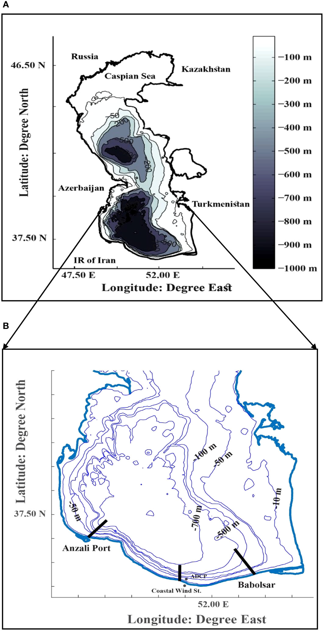
Figure 1 (A) The Caspian Sea: shallow water basin in the north, and deep basin in the middle and southern area. (B) The study area in the southern continental shelf of the Caspian Sea with measurements transects, ADCP st. and coastal wind st. in the southern coast.
In order to observe flow data and physical components of seawater, Doppler Current Profiler-WHS and Idronaut Ocean Seven 316 CTD profiler were used. The instrumental measurements on the current by the ADCP-WHS profiler were carried out in the southern boundary of the Caspian Sea (shelf zone). The recorded time series can describe higher frequency characteristics of the current (seawater dynamics). Useful knowledge about hydrodynamics and general water circulation in the region can obtain based on observed data analysis methods. The current meter (profiler) was set up with a time interval of 10 min. The device was installed on the continental shelf using a special stainless still frame at about 21 m depth (at approximate coordination of 51°27’9.45”E & 36°43’24.88”N). The current meter was deployed as upward technique on the sea bottom. Physical parameters of seawater were measured by CTD device in self-recording profiling method. The CTD profiling fixed stations were at a regular spatial resolution of about 1.5 km. The CTD probe was sent down by the wire and winch of the research vessel in the water column with a time interval of 1s. Furthermore, in order to better evaluation on the hydrophysical conditions of the southern coastal waters, the data of two transects in eastern and western areas were also assessed. The position of measurements transects, ADCP station and coastal wind station is shown in Figure 1B. The in-Situ measurement points were chosen to cover the physical characteristics of seawater from the shallow area near the shoreline to the deep areas far from the shore. Also, different areas in the central, eastern and western parts of the study area were considered and investigated. The depth of the measuring stations has increased from about 5 m in the shallow area to intermediate and deep waters (max. 600 m depth). The time duration for measuring the physical parameters was monthly and in this research the conditions of the indicative months and seasons are presented. The volume of hydrophysical data casts collected in the eastern, central and western parts of the southern boundary of the sea was large. Then, the generalization of the results was done based on all the measured and recorded data for the waters of the southern border of the Caspian Sea (2008 -2018).
The characteristics of the wind components in the region were obtained from a meteorological station installed at the height of 10 m on the south coast (051°27′53″E & 36°39′48″N). The position of the station was considered near the position of current meter in the middle part of the southern coast near Nowshahr Port. The alongshore and cross-shore components of wind (the U and V components of the wind in the region during the data collection time period, December 2017 to February 2018) were used. During the study the current direction is the direction to which the sea currents are going while the wind direction was defined as the direction from which the wind is coming.
The investigation of the vertical structure of the water column was based on the results of the hydrophysical data collected from 2008. In order to study the wintertime flow pattern in the southern part of the Caspian Sea, the current profiler data was recorded from December 2017 to February 2018. Time series, spectrum and roses were applied to analyze the current data. Furthermore, vertical structures of seawater parameters and cross-correlation were used on the collated data. The collected data were quality controlled after collection, and the results were compared with those provided by similar research. Therefore, the analysis results are completely certain of the input data.
2.2 Cross-correlation function (analysis)
Cross-correlation analysis is a method to examine the similarity and relationship between two-time series data such as wind and current. To investigate the relationship between the local wind and the flow pattern, correlation analysis, and rose diagrams were performed on the collected data. Normalized Cross Correlation Function (N-CCF) has been used to assess the collected time series data of current at various depths. The normalized Cross Correlation Function is a standard examination method for computing the association (or relationship) between different time series or parameters (Wei, 2006). N-CCF technique is used in a wide variety of data analyses, especially in marine and ocean sciences, meteorology, and earth sciences (Campillo and Paul, 2003; Capello et al., 2016; Thouvenot et al., 2016, (Emery and Thomson, 2001). In this research, the NCFF analysis technique was applied to investigate the effect rate (dependency or non-dependency) of the regional wind on the mechanism of creation of sea currents. In other words, the correlation between wind and seawater dynamics (current, …) components in the region was analyzed.
Some techniques have been applied for data analysis during this research such as cross correlations analysis, time series and spectral analysis. The formulation for NCFF analysis is as follows.
As stated in textbooks and articles, Normalized Cross Correlation Function (N-CCF) is presented and computed as following formulas (Emery and Thomson, 2001) (Equations 1–3):
And also,
Where x1(t) and x2(t) are two different series to compare.
It is also necessary to explain that CCF is applied as the next formulation for digital records, and w(n) and z(n) are two discrete time records and signals.
2.3 Quantifying the Water Column Stratification
The Richardson number is an amount of relative importance of mechanical and density effects in the water column. It is defined as the ratio of buoyancy gradient or frequency to the velocity shear (which can be reason the turbulent mixing) as follows (Equation 4).
where Ri is Richardson number, N is the Brunt-Väisälä frequency, ρ is the seawater density and g is the gravity acceleration (Knauss, 1997; Emery and Thomson, 2001). During this study, the water stratification was evaluated and quantified based on the Buoyancy frequency, velocity shear and Richardson number.
3 Results
3.1 Hydro-dynamical evaluations, variability of current
Time series of alongshore and cross-shore components of current and direction and magnitude current components at the surface layer was presented in Figures 2A–E. Collected data was presented as a time series with a time interval of 10 min. The component perpendicular to the shore (cross-shore) of the current is mainly recorded with changes and with a lower intensity and speed than relative to the component parallel to the shore (alongshore). As can be seen in the Figure 2, the speed of the parallel and perpendicular components of the current at some times during the measurement period were mostly close to one ms-1. The collected data results show that sea currents in the surface layer have recorded significant changes up to the value of about 1.058 ms-1.
Figure 2 (A) Time series of alongshore component (U) and (B) cross-shore component (V) of current at the surface layer, (C) current velocity magnitude (D) UV components of current at the surface layer (E) vector diagram of main (total) current (no separated into U and V components) observed at the surface layer.
U and V time series are shown in one graph to compare the components parallel and perpendicular to the coast. Also, the stick plot of the flow time series during the measurement period can be seen well. The diagram distinguishes the ranges of changes in flow speed and direction during the measurement period. According to the recorded data, the flow speed was around 1 ms-1. But sometimes, peaks higher than 1.5 ms-1 have also been recorded. Most of the peaks and strong currents occurred in the winter season (January and February).
The spectral analysis of surface current data for U and V components is showed in Figure 3A. During the measurements, number of current data was 8103 and Nyquist frequency was calculated as (fn=1/(2 Δt)=1/(1200s)). High values in both components (parallel and perpendicular to the coast) were related to the lower frequencies and, in other words, to periods of about one day or more (Figure 3A). Therefore, it seems that the flow components with smaller periods have much less energy and were less effective in the continental shelf region. Figure 3B presents the spectral analysis of the continental shelf region’s time series of surface flow data. Both phase and coherence elements were given separately in the graph for the flow data. The results clearly show that the velocities parallel to the shore were predominantly stronger than those perpendicular to the shore during the period. The comparison of the values and direction of flow showed that the flow direction in the east-west direction was mainly from west to east (the stronger currents were recorded in the mentioned direction). The absolute value of the component perpendicular to the coast was between +_1 ms-1, while the velocity values in the east-west direction often varied between +_1.5 ms-1. The spectral analysis indicated that the density of currents with lower frequency or longer periods was more in different directions. The results show the fluctuations and different peaks of current with different frequencies as a ratio of cycles per hour.
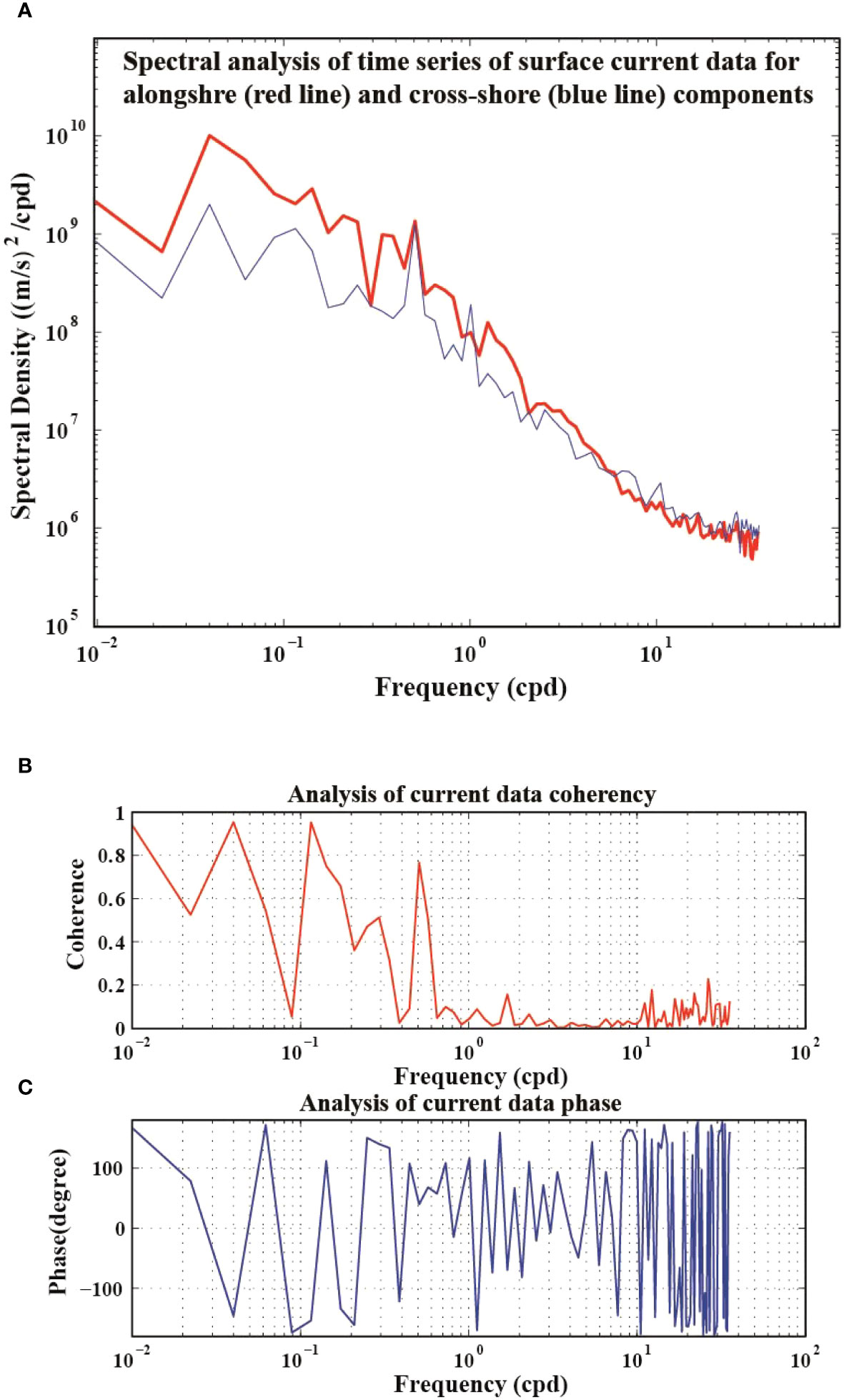
Figure 3 (A) Spectral analysis of time series of surface current data for alongshore and cross-shore components (the alongshore component is shown in red and the cross-shore component is shown in blue), (B) cross-spectral analysis (coherence analysis) and (C) phase analysis) on the current data. The unit of horizontal axis is cycle (time) per day (cpd) or time/day (Emery and Thomson, 2001).
The findings clearly showed that the strong surface currents have occurred in the region. By comparing the flow conditions at the surface and the lower layers, it was observed that the flow intensity values decreased with increasing depth. The analyzes showed that the coherence of current occurrence with lower frequencies was significant and nearby to 1, and the currents with higher frequencies had a coherence close to zero. While currents with different frequencies have been recorded in different directions. It means that, there have been changes in the flow direction in the studied area both in events with short time periods and in long time periods (Figures 3A, B). Although this change in the flow direction was recorded more in higher frequency flows. The change of phases and the occurrence of flow in different directions in Figures 2, 3 have been clearly seen.
Monthly average values, standard deviation, monthly maximum, and range of components changes parallel and perpendicular to the coast are presented in Table 1. During the entire period, the measurements showed high values of monthly average along U direction (Figure 4). The highest average monthly value of the component parallel to the coast of the currents was observed in January. Also, the highest average monthly value of the component perpendicular to the coast of the currents was in January. The maximum value of the component parallel to the coast of the surface currents in December, January, and February is about 137, 200, and 139 cms-1, respectively, and the maximum value of the component perpendicular to the coast of the surface currents in the same months is about 106, 169, and 96 cms-1, respectively. In January, the first month of winter 2018, the currents parallel to the coast (alongshore current) intensified. The average monthly components of surface currents parallel and perpendicular to the coast were estimated as 68.7 and 33.7 cm/s, respectively.
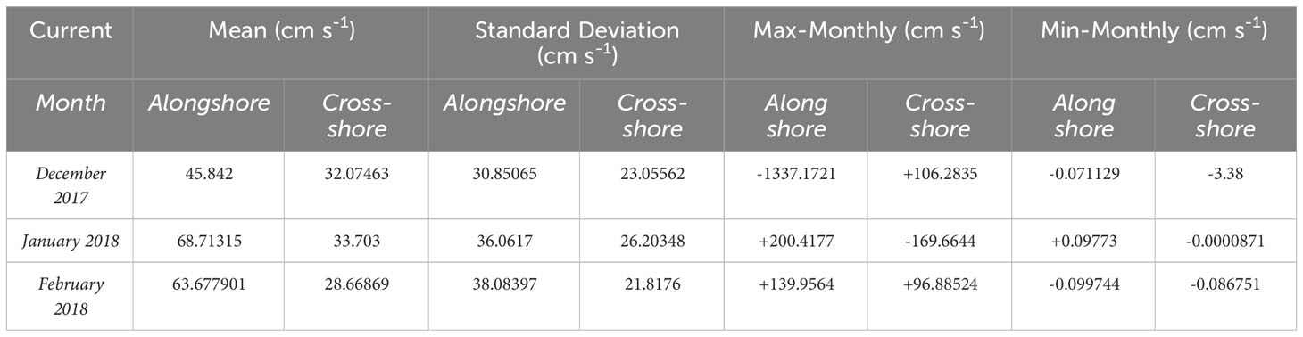
Table 1 The summary of current components in duration of measurements.
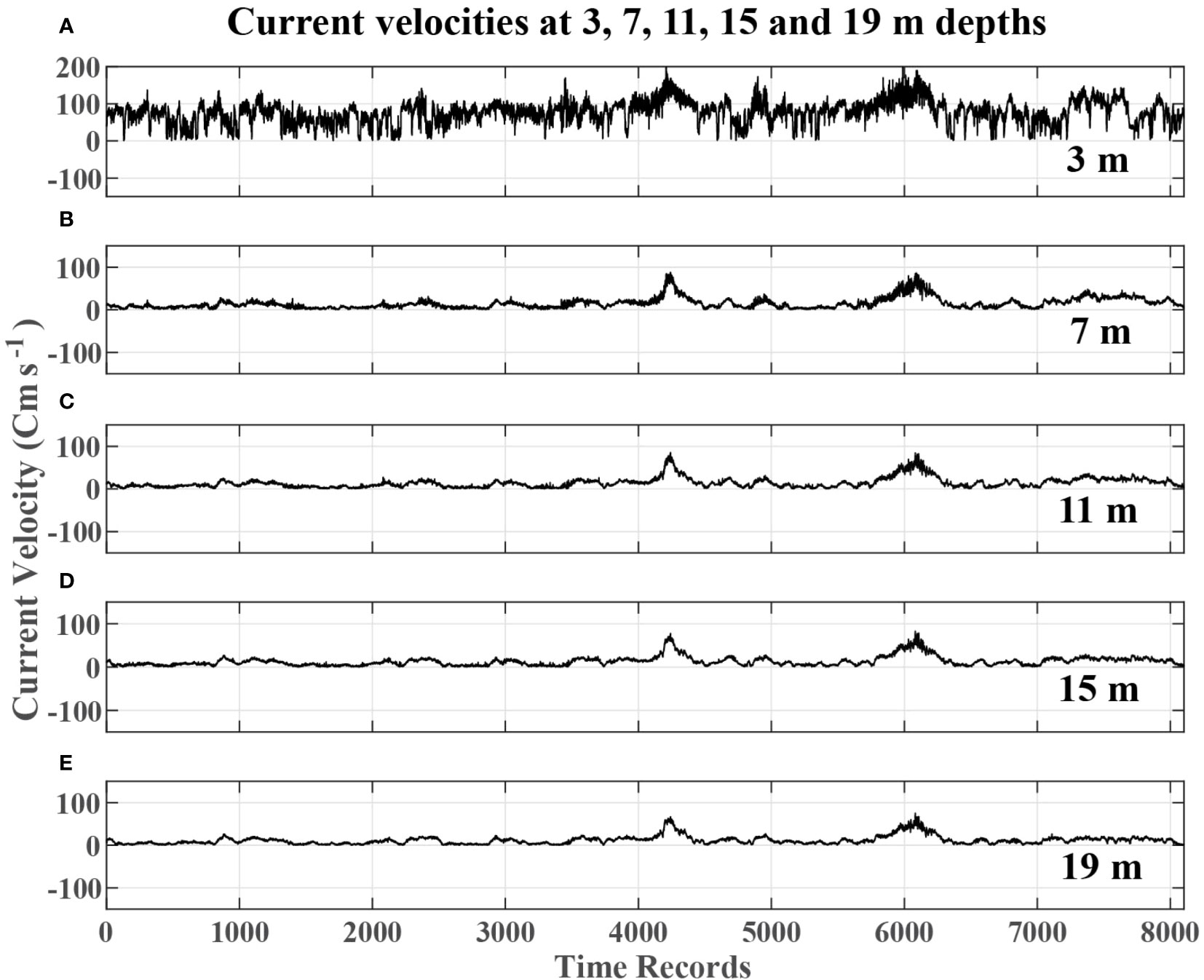
Figure 4 Time series of current velocities during the period of observations at (A) surface (upper 3 m layer), (B) 7 m, (C) 11 m, (D) 15 m and (E) 19 m depths (data recorded between December 2017 to February 2018).
As can be seen in Figures 3A–C and 4, the energy of alongshore current (parallel to the Iranian coast) is mainly concentrated in periods of longer than one day. In the autumn (December), alongshore currents and their fluctuations are intense. The daily values of current up to one ms-1 were observed. At the beginning of the winter season (January), the currents and fluctuations were stronger than those during the previous month. The maximum velocities values generally displayed an increasing trend compared to those in December. The analysis results on the collected data showed that the currents with low-speed oscillation frequencies were dominant in the studied area during the period of the observations. According to the values in Table 1, there has been an average residual current in the region from west to east. The residual current’s absolute velocity value has been variable during the measurement period. The average value of the alongshore component in February was 63 cms-1, and its minimum value was about 0.0997 cms-1 in January. The average velocity of the cross-shore component (perpendicular to the Iranian coast) in February was about 28.6 cms-1.
To study and achieve an accurate comparison, different components of the flow profile in different layers of the surface, 7, 11, 15, and 19 m depths, have been analyzed. So, time series diagrams of monthly variations of current velocities and directions observed at the layers of the sea surface, 7, 11, 15, and 19 m depth, were displayed in Figures 4A–E. The results showed that the sea currents in the region near the surface were much stronger and more intense than the lower layers. It means that a significant difference was observed between the characteristics of surface and deeper layer currents. The intensity of the sea current clearly decreased with increasing depth. This could be due to the influence of currents on wind and kinetic energy from the atmospheric conditions over the sea. It is important to note that the speed and energy of the flow components decrease at lower levels near the seabed, which can be affected by the friction factor of the seabed (Figures 4A–E, 5A–E, 6A–E).
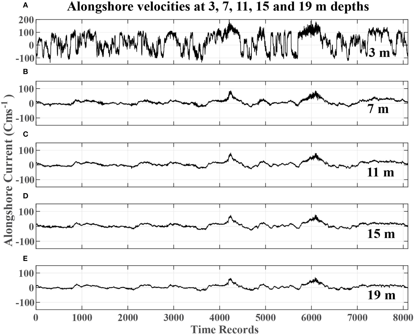
Figure 5 Time series of alongshore component at (A) surface (upper 3 m layer), (B) 7 m, (C) 11 m, (D) 15 m and (E) 19 m depths (data recorded between December 2017 to February 2018).
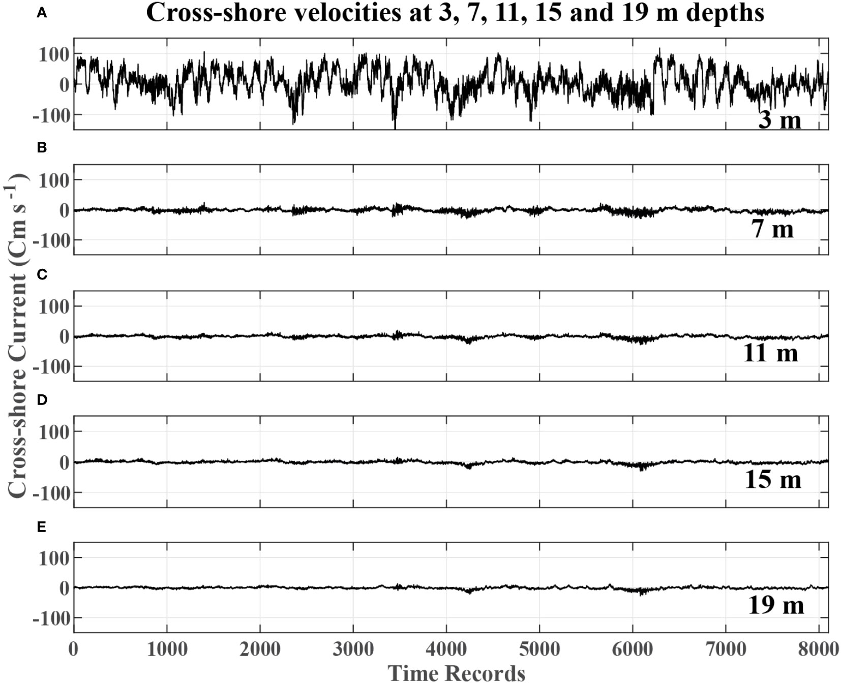
Figure 6 Time series of cross-shore component during the period of observations at (A) surface (upper 3 m layer), (B) 7 m, (C) 11 m, (D) 15 m and (E) 19 m depths (data recorded between December 2017 to February 2018).
The vertical changes of current in coastal waters and continental shelf usually have a complex pattern and are influenced by various factors. Mainly, the dynamics of the water column is influenced by different elements. In the analysis of the results, evidence of large circular rotations and wind-induced currents are generally identified. The movement of sea water does not have a simple pattern and the water column is not only directly affected by the wind drag on the surface. The factors such as stress shearing friction, roughness of the seabed, Ekman spiral (motion) and friction between different lower layers of water cause energy consumption and weaken the intensity and speed of the flow in the water column.
Comparison and assessment of rose diagrams showed some variety in the directions in the water column from surface to lower layers during the observation period. Results showed that sea currents were generally oriented north, north-west, and east at the surface layer. They can sometimes be observed to the south (coastline). It means that the cross-shore component was strong at the sea surface level. With moving to the lower layers in the seawater column, the dominant flow directions were toward the north-west and southeast during December. Analyzing the observed data at the different levels over the shelf displayed that the dominant direction at 7, 11, 15, and 19 m depths was north-northwest in the first month of winter (January). During the measurements in various months, a general similarity in the directions at 7, 11, 15, and 19 m depths has been visible in the graphs. The maximum velocities up to 200 cms-1 are clearly observed in the time series in January and February (Figure 4A). Based on the time series, the speeds and directions of the current at the subsurface level were not uniform (with high frequency). The figures specified the changeability of directions with a small dominance to the northwest and sometimes, to the south at the sea surface.
Examining the fluctuations in the time series of the flow components from the surface to near the seabed and the values presented in Table 1 explains that there is a residual flow to the east and parallel to the southern coastline. This event has also been confirmed by Zaker et al. (2007) in the eastern part of the South Caspian Sea. Depending on the sea conditions and different months, the residual eastward flow varies in intensity and speed during the measurements. The investigation of the vertical flow profile in the time series has revealed two peaks of the flow during the storm in the alongshore component (observed from the surface to the depth in all layers). This event has been seen as extreme fluctuations in the cross-shore time series. The average values of the alongshore current parameter in December, January, and February were more than 0.45 ms-1, 0.68 ms-1 and 0.21 ms-1, respectively. The comparison of time series of measured current data in numerous layers (surface, 7, 11, 15, and 19 m depths) displayed that alongshore components were homogeneous in the study area. The along-shore element of the flow was dominated by low-frequency oscillations during the project duration. Alongshore components had monthly variations with maximum monthly magnitudes of 2 ms-1 and 1.39 ms-1 in January and February (Figures 5A–E, 6A–E).
During the data recording period, the cross-shore component has always been weaker than the alongshore component. Based on the results, the general direction of water flow in the southern shelf was mostly from northwest to southeast (and east). The factors that can be effective in creating this phenomenon are the general circulation regime of the southern basin, the wind in the area, and the topographical structure of the seabed. The vertical profile of the flow velocity usually varies (decreases) from the surface to the bottom, and the highest velocity was at the surface. Based on the analysis of recorded hydrological data (CTD casts) and ADCP current-meter values, an upwelling event related to the wind over the area was not observed. By comparing the components of wind and current (time series), it seems that there was often no proper correlation between them (except in some storm cases). The weak correlation between the wind components and regional currents strengthens the possibility that another factor (such as basin scale cyclone) can create marine currents effectively. Previous research has reported on the effect of the general water circulation in the southern basin of the Caspian Sea on the water dynamics of the southern coastal waters (Kosarev, 2005; Tuzhilkin & Kosarev, 2005). The results of statistical evaluations (Table 1) showed the mean values of cross-shore components up to 0.33 ms-1 during the records. Generally, the alongshore and cross-shore components of the flow in the winter season were considerable. Monthly eastward alongshore flow speeds were calculated up to 0.69 ms-1, which can reveal the effect of the southern basin scale cyclone. Some researchers, such as Tuzhilkin and Kosarev (2005) and Zaker et al. (2011), reported the hypothesis of creating coastally trapped waves on the sea’s southern border.
3.2 Wind variability
Figures 7A, B shows the wind condition in the region during the observations and measurement of current. Table 2 shows summary information on wind, such as monthly average and standard deviation on velocities. In December, the wind direction was mainly from the west and northwest, although weak winds from the southwest and southeast were also recorded. The wind speed is mostly below 5 ms-1, but sometimes it reaches about 6 ms-1. The speed of the alongshore wind component was mostly higher than the speed of the cross-shore component. The daily average velocity of the cross-shore component of wind was mainly between 1 and 2 ms-1 and sometimes up to 3 ms-1, while in the direction of the alongshore wind component, speeds ranged between 2 and 4 ms-1. In January, the wind was mainly from northwest and west. Sometimes weak southeast winds were also observed. Wind speed and intensity were often stronger than in December (more than 4 ms-1). Stronger winds with speeds up to 14 ms-1 have also been observed from the northwest direction (in most of the data, it was between 2 and 6 ms-1). The alongshore component wind was more intense than the component cross-shore, with a monthly maximum of about 14 ms-1. In February, the wind was mostly in the north-west direction; in other directions, it was weak with low intensity. It has been stronger in the northwest direction with an average speed of 1.5 ms-1 (alongshore component) and an average speed of about 1.55 ms-1 (cross-shore component). During January, the wind intensity in the alongshore direction (with a maximum of 11 ms-1) was higher than that in the cross-shore component (with a maximum of 4.49 ms-1). During the measurements in February, the mean alongshore wind speed component in the region was stronger than in January. In contrast, the maximum wind velocity was logged in the first month of winter (January). The wind rose diagram and current rose diagrams are presented in Figures 8A–F, 9A–F, 10A–C, 11A, B. The dominant wind direction over the region mainly originated from north and northwest. The strong winds arrived from a north direction on the southern continental shelf. The changes in wind directions were considerable; about 12% of winds come from the southwest (speed up to 12 ms-1). Notably, the northerly winds were dominant, while more than 5% of winds were from the south direction. A comparison of the wind and flow rose diagrams shows that strong winds were mainly from the north and northwest, while the stronger currents were mainly towards the north. Lower speed winds and weaker sea current were recorded in the northeast and south directions.
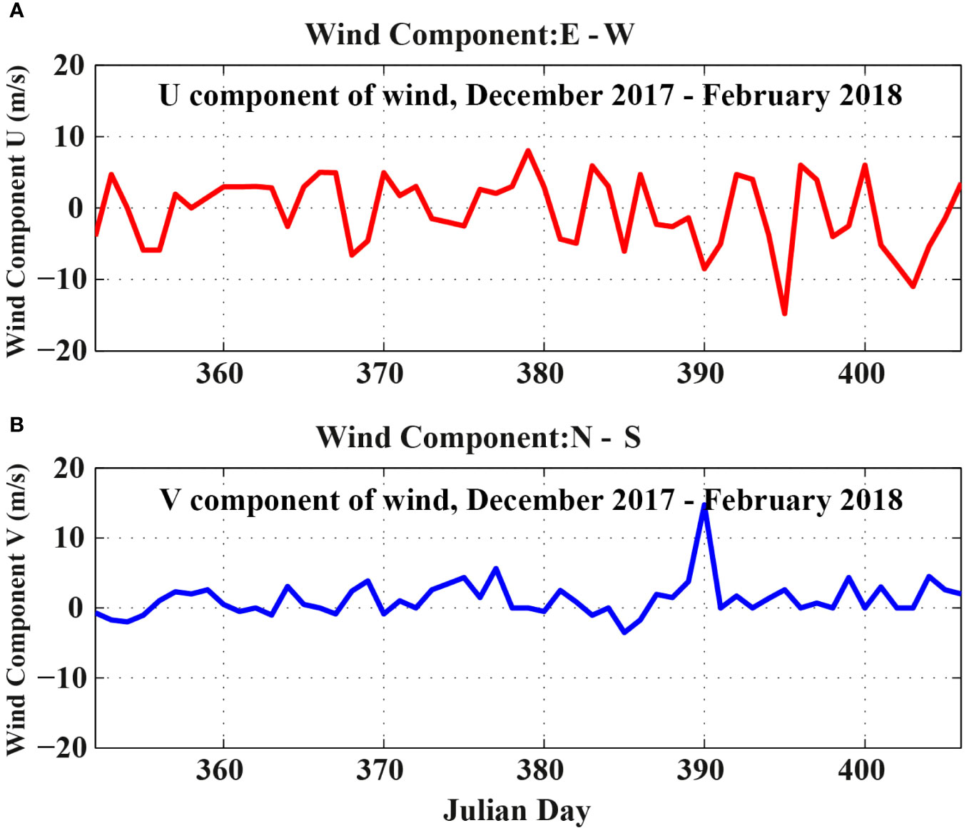
Figure 7 Time series of wind component, (A) U and (B) V in the southern slope of the Caspian Sea (Julian days were used to recognize and distinguish the measurement period, December 2017 - February 2018).
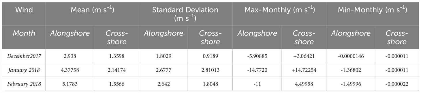
Table 2 The summary of wind components in duration of measurements.
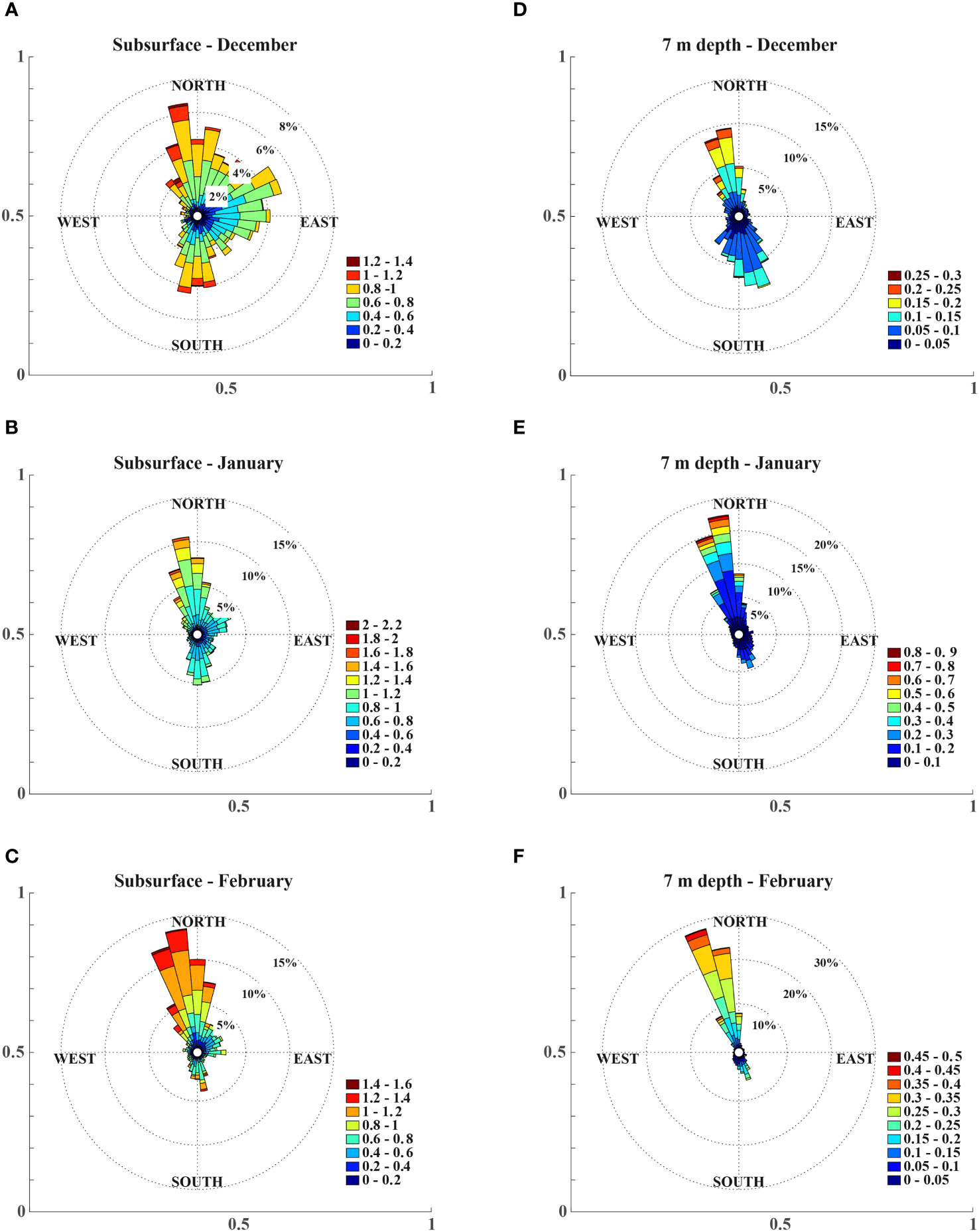
Figure 8 Current roses (speeds in ms-1) at surface in (A) December, (B) January, (C) February and at 7 m depth in (D) December, (E) January, (F) February in the southern shelf of the Caspian Sea.
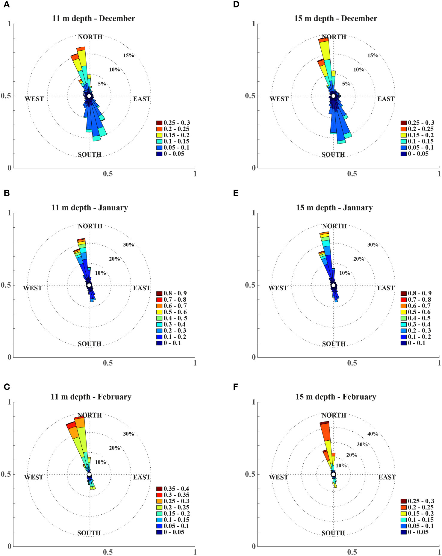
Figure 9 Current roses (speeds in ms-1) at 11 m depth in (A) December, (B) January, (C) February and at 15 m depth in (D) December, (E) January, (F) February in the southern shelf of the Caspian Sea.
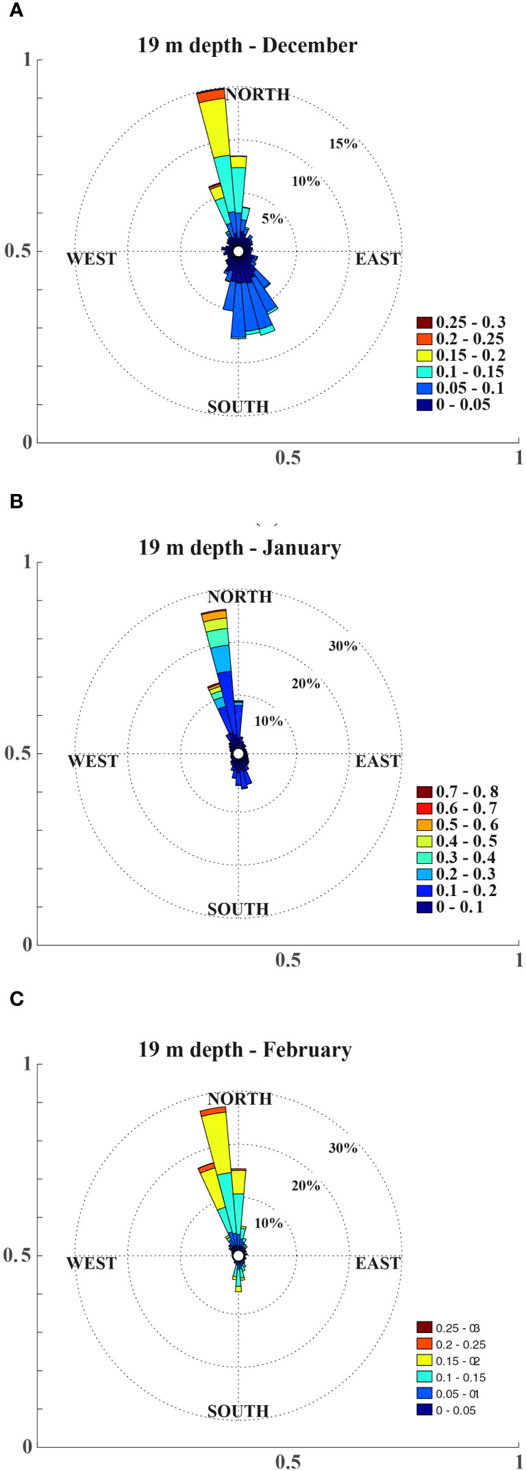
Figure 10 Current roses (speeds in ms-1) at 19 m depth in (A) December, (B) January, (C) February in the southern shelf of the Caspian Sea.
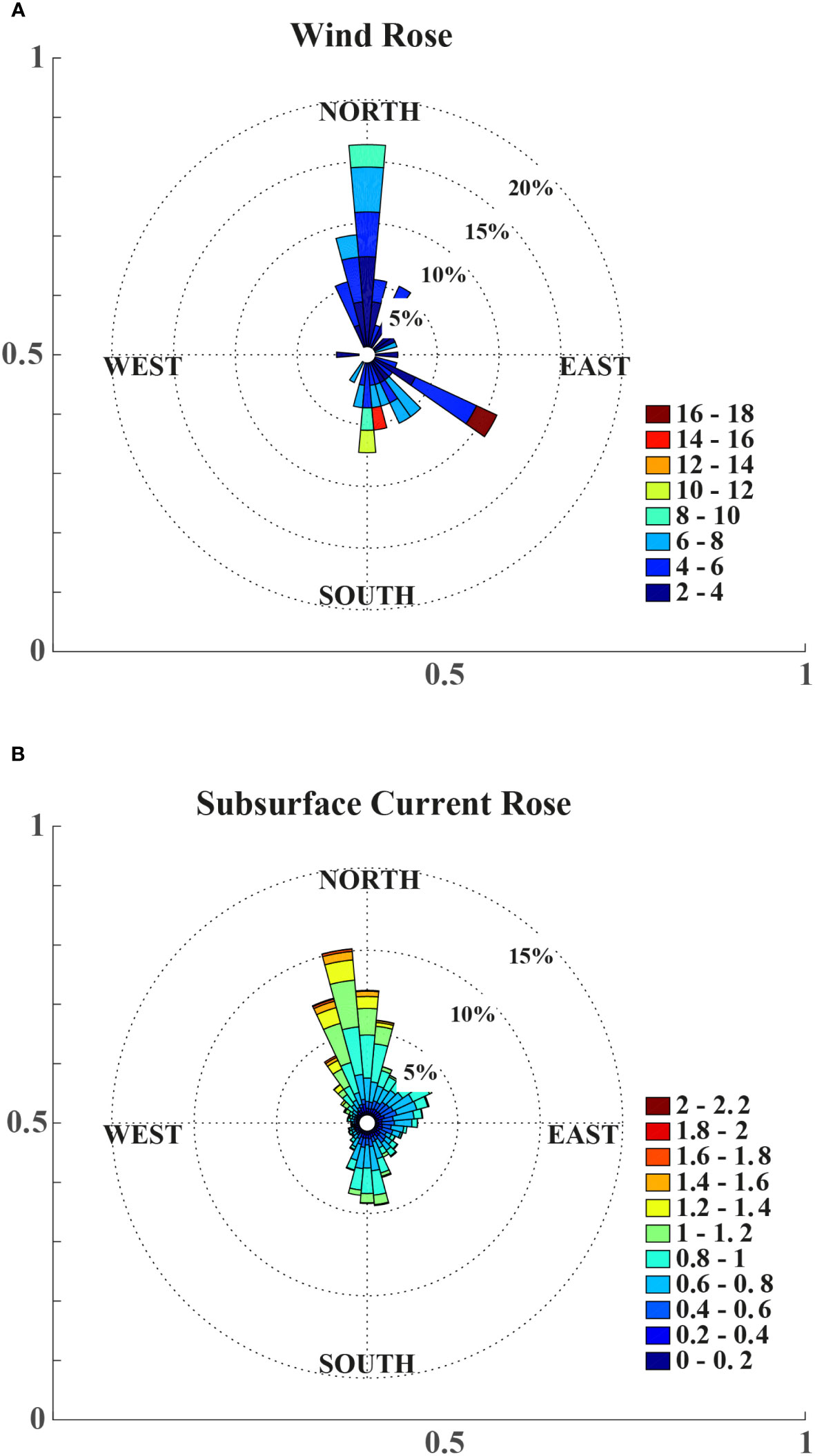
Figure 11 (A) Rose diagram of maximum wind velocities (ms-1) at a coastal weather station in the study area and (B) current rose (ms-1) at surface layer.
The average values of the alongshore current velocity in January and February were more than 68 and 63 cm/s, while the cross-shore speeds were more than 33 and 28 cm/s. This means that the alongshore component was stronger than cross-shore component. The values of the alongshore and cross-shore components of the speeds over the continental shelf were up to 200 cm/s (with both positive and negative signs). Throughout the entire duration of measurements, the direction of components of sea flow was sign-alternating. During the observations, winds by variable strength up to 10 m/s were recorded almost exclusively from north and northwest directions (dominant in winter in the area) (Terziev et al., 1992; Zavialov et al., 2022). However, in a few cases, a strong wind with a speed of up to 18 m/s was recorded from the southeast (Figures 5, 6).
3.3 Correlation and dependency
The monthly current rose for various water column layers during the observation period was presented in Figure 6A. It can be clearly seen that the current surface rose was stronger than those in the lower levels. The changes of flow direction during December in the study area were higher than variations during January-February. The current roses diagrams showed the northeasterly and southwesterly dominate sea currents directions (Figures 8A–F, 9A–F, 10A–C, 11A, B). In the southern part of the Caspian Sea, sea storms were often observed between mid-autumn and mid-winter. The cross-correlation coefficient calculated for the observed alongshore component (U) of the current at the surface layer and alongshore local wind velocity was r=0.11. Similarly, the coefficient computed for the cross-shore components (V) of surface current and wind was about 0.18 for the time of measurements. Generally, the trend of current components at various levels of the water column showed similar behavior. However, they become stronger as they approach the sea surface. The cross-correlation coefficient computed for surface alongshore components and alongshore element of flow at 11 m depth was approximately r=0.55, and for cross-shore components at mentioned layers was more than r=0.35. Comparison the correlation coefficients of velocities recorded at the sea subsurface layer and 19 m depth displayed a descending trend (coefficient for alongshore component r=0.51 and cross-shore component were more than r=0.18). According to the poor relationship between the flow components at sea surface and the local wind, other effective and stable factors were involved in the generation and changes of currents in the southern continental shelf region. For instance, another moving mechanism, such as the general pattern of southern basin circulation, can be effective.
3.4 Hydrophysical studies
Based on the results of the present (Figures 12A–D, 13A, B) and previous observations (Jamshidi and Bakar, 2012; Jamshidi and Jafarieh, 2021; Jamshidi and Yousefi, 2021), usually, the temperature of the surface layer of the sea in the middle of summer is about 29°C, which reaches about 24°C in October (autumn). In the middle of summer, the thickness of the surface mixed layer is about 20 m, while it reaches about 35 m in the middle of the autumn season. In terms of vertical temperature changes, the thermocline (and also pycnocline) layer was observed with a thickness of 30 m with 16 degrees changes in the middle of the summer season, and consequently, with a thickness of 15 m and vertical changes of about 10°C under the surface mixing layer and at the end of October (Jamshidi and Bakar, 2012). Due to the low vertical changes in water salinity (the range of seawater salinity between 12-13 psu, Figures 12A–D, 13A, B), the vertical changes in seawater density were correlated with vertical changes in seawater temperature (Jamshidi and Bakar, 2012). The deep-water layer is located under the thermocline layer with low seasonal changes in temperature and salinity (Tuzhilkin and Kosarev, 2005; Jamshidi, 2022). The results of measurements of physical properties such as temperature, salinity, and sigma-T are presented in Figure 12A–D. Variations in thermal and density stratifications are clearly observed in the multi-axis’s diagrams (for more information and comparison, refer to Ambrosimov et al., 2011; Dyakonov and Ibrayev, 2019; Zavialov et al., 2022).
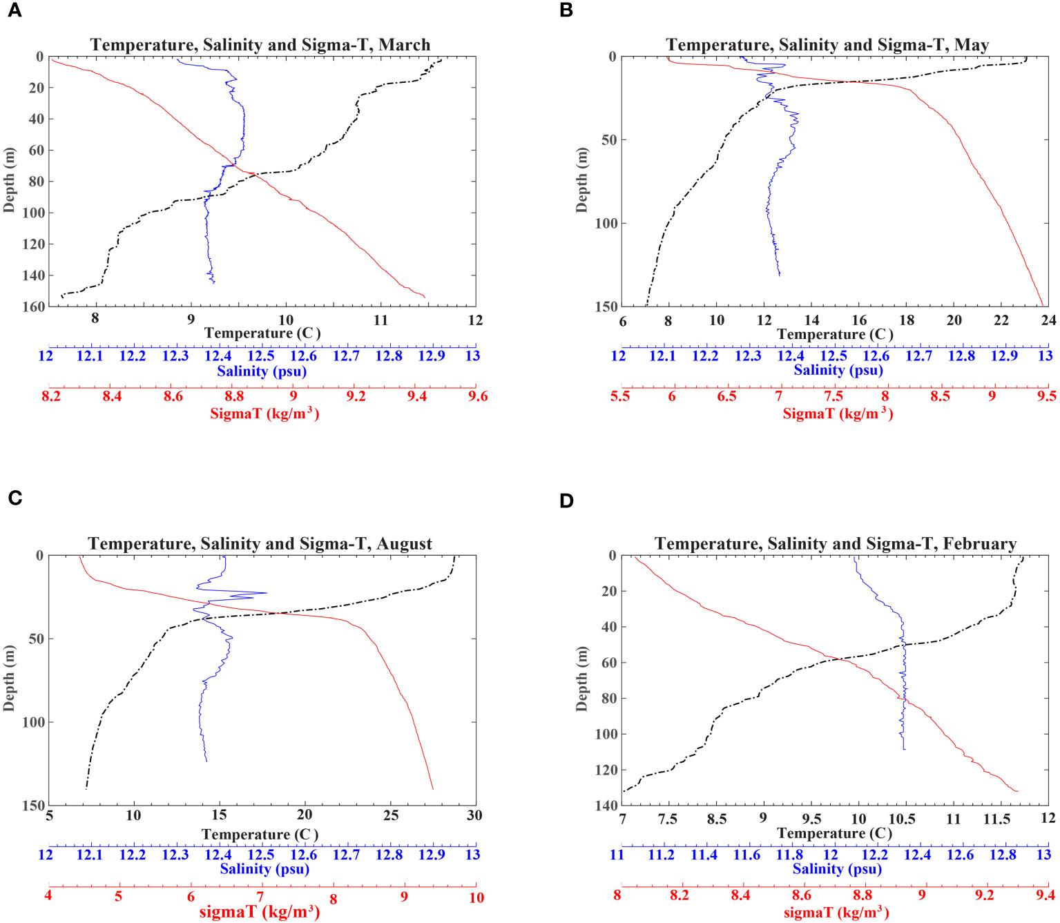
Figure 12 Vertical changes in temperature, salinity and sigma-T and stratification in (A) March, (B) May, (C) August (D) February near Nowshahr port in the center part of the southern coast of the Caspian Sea.
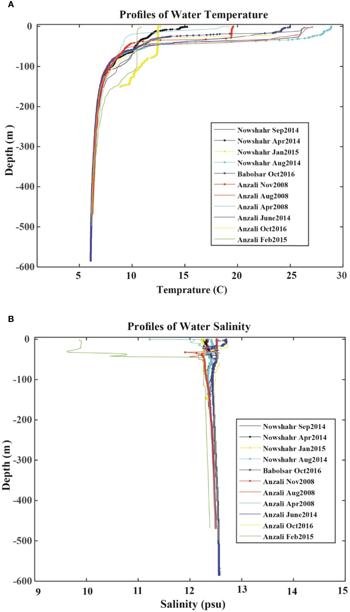
Figure 13 Vertical changes of (A) temperature and (B) salinity during different years near Anzali port in west, Nowshahr in center and Babolsar in eastern areas of the southern border of the Caspian Sea.
4 Discussion
The results of the study on the flow pattern, wind, and changes of the physical seawater parameters in the southern continental shelf of the Caspian Sea were evaluated. Regarding the component perpendicular to the coast, the directions of the current to the north and south can be distinguished. The peaks with the maximum values of the flow velocity in the winter season can be well recognized in at least three cases. The observed fluctuations and peaks during winter storms can be caused by the influence of strong winds and the increase in the kinetic energy of the upper layers of seawater in the region (Figure 2). Due to the increase in the kinetic energy of seawater and the phenomenon of winter storms in the region, it is expected to create strong currents in the waters of the southern border of the Caspian Sea. During the measurements, the cross-shore and alongshore components of the current velocity had various signs. They showed changes almost at all layers from the surface to the bottom in the vertical profile. Due to the friction of the seabed, the coastal currents in the horizontal direction often have a vertical shear which decrease the speeds from the sea surface to the bottom (Li et al., 2009). The low correlation between wind and current indicates the effect of other dominant factors in variability in the pattern of directions and speeds.
The results of cross correlation analysis and spectral analysis showed that at some times in the period of late autumn and early winter, the coordination between wind (stress force) and current was weak, and at some times, in the absence of any strong wind, large currents parallel to the coast line were observed. The absence of dependence and correlation between the wind factor and sea current in the study area, as well as the presence of currents with significant intensity when there is no strong wind raises the question that, what is the reason of the observed flow on the southern continental shelf? Or what is the probable sources of sea current generation based on the predominant energy frequencies? The conditions observed during the measurement period and the pattern of the current parallel to the coast strengthen the hypothesis that the conditions for creating a phenomenon called coastal trapped waves have been created. These types of seawater movement, which are barotropic and have been created and observed in many areas of the continental shelf, have a major effect on changes in the pattern of sea currents. The mentioned phenomenon is one of the main characteristics of most of the shallow continental shelf. It is necessary to pay basic attention to them when studying sea currents in coastal areas. The presence of a sloping continental shelf causes the generation and propagation of waves that leave the area of the periodic wind force and is observed as a periodic movement of water in a place further away on the coast where it is outside the strong wind field. On the southern shores of the Caspian Sea, there is a continental shelf with a suitable slope and it is possible to create the mentioned phenomenon (Csanady, 1997; Tomczak and Godfrey, 2003). During the previous texts about the Caspian Sea reported the possibility the existence of oscillations with periods of one-three weeks related to the coastal trapped waves (Tuzhilkin and Kosarev, 2005).
The corresponding components of the currents at various water layers were not strongly correlated. It means that the characteristics of the current local structure were not well spread at the entire water column. It seems that the effect of basin-scale dominant cyclonic structures expanded over the southern continental shelf. A similar condition has been mentioned in previous research on the Caspian Sea (Tuzhilkin and Kosarev, 2005; Zaker et al., 2007; Bohluly et al., 2018; Dyakonov and Ibrayev, 2019; Rahnemania et al., 2022). Based on the previous studies, there are basin size cyclonic and anti-cyclonic gyres in the southern, central and north Caspian Sea (Tuzhilkin and Kosarev, 2005). In general, there is a main background movement (current) in the southern Caspian Sea. The mean annual view of general water dynamics of the southern basin shows a dipole gyres in the region through the year. The anticyclone is formed in the northwest of the basin and the cyclone is located in the southeastern part (near the Iranian border). In the vertical direction, flow velocity decreases from sea surface to below the location of seasonal thermocline layer (Tuzhilkin and Kosarev, 2005; Bohluly et al., 2018). Based on the results of previous studies, the monthly variation in the current pattern in the southern basin is under the influence of basin-scale gyres. In the winter, the anti-cyclonic gyre in the South basin is strong, and in summer, the cyclonic motions have the highest intensities. The maximum velocities in the mentioned sub-basin circulations reached 0.2m/s, while the speeds decreased to 0.05 m/s in deeper layers below 100 m (Tuzhilkin and Kosarev, 2005). The measurements revealed that the monthly flow changes in the region are significant and can be influenced by various factors. The area’s alongshore and cross-shore current elements have recorded extensive changes in the vertical profiles. The calculated coefficients for the correlation between the different flow components and the regional wind during the study period were low. This condition has already been reported in the results obtained in other regions of the southern Caspian Sea (Zaker et al., 2007). The data identify the feature of the study area’s current profiles and the wintertime patterns. Local wind continuous and stable role in the production and variability of currents in the southern continental shelf region was not recognizable. But it was different in stormy and extreme conditions.
The riverine discharge and atmospheric parameters determine the particular features in hydrological conditions and a general Caspian Sea water circulation pattern. Those elements create rapid and major long-term variability in this sea, much greater than other seas worldwide (Kosarev and Kostianoy, 2005). Due to the great seasonal changes of atmospheric parameters and their effects in the southern part of the Caspian Sea, temperature and fluid kinetic energy (air and seawater) changes are significant. The process of the vertical structure of Caspian Sea showed that the seawater column in the southern part of the Caspian Sea is stratified in warm months. The seasonal change of atmospheric parameters affects the vertical structure of seawater and thermal stratification. Although the influence of freshwater input in the mouth of rivers is considerable on the stratification pattern (Kosarev, 2005; Tuzhilkin and Kosarev, 2005; Zaker et al., 2007). Observations and vertical temperature profiles showed existence of a strong seasonal thermal stratification in the region (Figure 7; Jamshidi and Yousefi, 2021; Jamshidi, 2022). Significant changes (thermocline and pycnocline layers) were mainly observed across the upper and intermediate layers. Seawater temperature and salinity changes in the deep layers were few. The results obtained in this research were agreed the results of other studies in different sea areas (Tuzhilkin and Kosarev, 2005; Zaker et al., 2007; Zavialov et al., 2022). Evaluations of salinity and temperature recorded data showed that the thermohaline structure has vertical and horizontal non-uniformity near the river mouth region. Based on the measurements, no upwelling phenomenon was observed in different areas of the southern coastal waters. It seems that it is caused to the direction of the wind and the location of the coastline.
Formation and destruction of water column stratification is influenced by current, kinetic energy and turbulence of wind and wave as well as buoyancy force. It is generally scaled and expressed in terms of the Richardson number (section 2.3). In the other words, an important parameter to evaluation and determination the stratification and stability of water column is the Richardson number. It means that the Richardson number is an equation for explaining the relation between motion velocity and water column layering (stability and instability) (Cushman-Roisin and Beckers, 2011; Allahdadi et al., 2013). The smaller values of the Richardson number show that the greater the tendency for the mixing in water column. In the other word, small Richardson number amounts express the predominant effect of velocity shear across the water column, and the turbulence or kinetic forces preventing layering (Knauss, 1997; Emery and Thomson, 2001). Enhancing the value of Richardson number from a certain value (0.25) indicates the reduction of the effect of turbulence forces in sea water. Thus, for Richardson number greater than 1, buoyancy force (driven by the vertical water density gradient) dominates. In this condition, the stratification is assumed stable and very weak mixing occurs in seawater column (Knauss, 1997; Emery and Thomson, 2001; Allahdadi et al., 2013). The denominator of Richardson number equation shows the effect of vertical shear mixing caused by the water flow. So, the larger the vertical gradient of the water flow component, results the larger the denominator of the equation (see section 2.3). It implies a smaller Richardson number and a mixed (non-stratified) water column (Pond and Pickard, 1983; Knauss, 1997; Allahdadi et al., 2013). According to the seawater properties profile in winter and flow pattern discussed in the previous sections, a considerable shear effect was expected and upper layer of water column was well-mixed over the continental shelf. To be more quantitative, denominator of Richardson number and situation of water column stratification for various random time records during the measurements were compared and evaluated. Table 3 presents the values of the Richardson number denominator for various records during the observation. Mostly, the calculated denominator values were large, especially in late autumn and early winter measurements (December and January). This means that at those times, the vertical mixing of the water column was much stronger and the currents and turbulence mixed the upper layer well. Field observations and CTD data collected during different years in the southern part of the Caspian Sea have shown that the natural structure of the upper layer of the seawater column from November to late February (mid-autumn to mid-winter) is mostly mixed and affected by currents and turbulence (Tuzhilkin and Kosarev, 2005; Jamshidi and Yousefi, 2021; Jamshidi, 2022). Although the grade of mixing, the intensity of the currents and the turbulence of the water column were variable at different times of the measurement period, and the calculated values of the denominator of the Richardson number represented it. The computed results for the conditions of the physical structure of the water column based on Richardson number were in agreement with the results of analyses on collected data of parameters of temperature, salinity, and mixing rate. As mentioned before, an important parameter for evaluating the stability of the sea water column (or the vertical density gradient) is the Brant Vaisala frequency or the stability frequency () (Kosarev, 1990; Kosarev and Yablonskaya, 1994; Tuzhilkin et al., 1997; Ibraev et al., 1998; Ibrayev, 2001; Ibrayev et al., 2001; Tuzhilkin and Kosarev, 2004; Nasimi and Ghiassi, 2006; Zounematkermani and Sabbaghyazdi, 2010; Kitazawa and Yang, 2012; Cutroneo et al., 2017; Jamshidi, 2017; Medvedev et al., 2020). The stability frequency is also called stratification frequency. The analyzes showed that in the upper layers, the more intense vertical density gradient causes more fluctuations and was associated with a shorter period (within a few minutes). But in deep water layers, where the stability number is from 10-8 to 10-6, the fluctuation period is several hours. Considering the depth of the measuring stations, the effect of compressibility is not very noticeable and can be neglected. In agreement with the calculations made by Peeters et al., 2000 for the Caspian Sea, stability values were positive in most cases. The contribution of the vertical temperature gradient in the stability grade (density values) was significantly higher than the contribution of the salinity gradient in the water column. The results show high values of static stability in the first few tens of meters of the water column, which indicates the existence of a seasonal thermocline-pycnocline in the sea water column during the summer to begging of fall. The maximum value of the stability frequency in the surface layer in the middle of the autumn season was 0.01271 x 10⁻³ s-2, and its maximum value in the lower layer was calculated as 0.006213 x 10⁻³ s-2. Measurements in summer and early autumn indicate that stratification of the water column and density changes have caused an almost significant peak in seawater stability values. Stability frequency calculations in early autumn in the western part of the southern waters of the sea showed that the maximum value in the surface layer is about 23 m, it was about 0.005465x10⁻³ s-2. While the stability frequency at the same time showed that the maximum value in the eastern part of the southern coastal waters at a depth of 17 m was calculated to be about 0.077586 x 10⁻³ s-2 and very little fluctuations were created in the lower layers. It was concluded that the peak of fluctuations or the maximum fluctuation of stability frequency was recorded at the border of two layers of surface mixed and thermocline in the warm seasons of the year. Therefore, it was concluded that when there was no strong stratification in the water column (late autumn to mid-winter), the frequency of buoyancy was high (without high peak values).
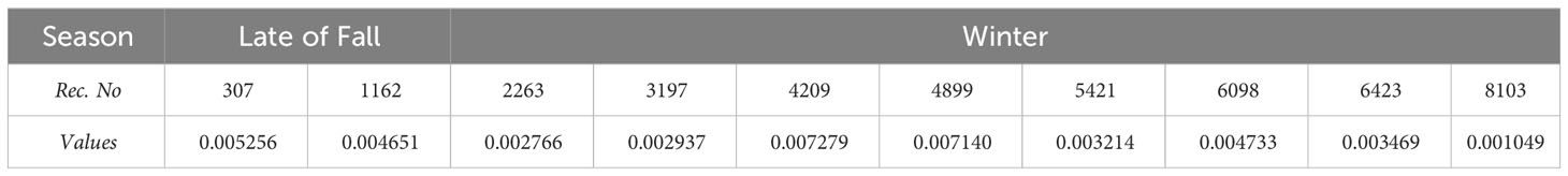
Table 3 values of denominator in Richardson number equation based on measured current.
5 Conclusion
The fall and winter flow characteristics over the southern continental shelf of the Caspian Sea were studied in terms of induced factors and their effects on the water column structure and stability. This study was conducted based on the analysis of current and wind data. By examining these data sets, researchers aimed to understand the factors that influence the flow patterns during the fall and winter seasons in the region. The collected data of the seawater physical parameters in the southern basin of the Caspian Sea during the monitoring period was utilized to expand the field of analysis. The recorded current data revealed significant monthly variations in sea surface velocities. As a result, the speeds and directions of the flow exhibited substantial changes in different months throughout the measurement period, both horizontally and along the vertical profile. These findings highlight the dynamic nature of the sea currents in the region and emphasize the importance of considering temporal variations when studying the oceanographic conditions of the southern basin of the Caspian Sea. The analysis of these changes provides valuable insights into the complex dynamics of the seawater and its flow patterns. During the beginning of winter, specifically in January, the current time series exhibited stronger behavior compared to other times in the southern basin of the Caspian Sea. This indicates that the flow velocities during this period were more intense, particularly in the upper layers of the water column. In contrast, the values recorded in the deeper layers showed relatively lower flow velocities. As a result, larger vertical gradients of velocity were observed in the water column during this time. This information suggests that the winter season, particularly in January-February, is characterized by more vigorous and pronounced current patterns in the southern basin of the Caspian Sea, with notable variations in velocity across different layers of the water column. The higher speed gradients observed during the monitoring period led to smaller Richardson numbers, indicating a higher degree of mixing within the water column. These conditions were particularly pronounced during sea storms and strong winds in the region. As a result, high current speeds were recorded during these events. The intensified mixing and increased current speeds can be attributed to the turbulent nature of the water column caused by the strong speed gradients and the influence of storm events. Indeed, several factors contribute to the flow pattern in the region of the southern continental shelf of the Caspian Sea. These factors include the topographic conditions of the sea bed, non-homogeneous changes in the width and depth of the continental shelf, the general circulation of seawater, and the wind fields. These elements collectively influence and shape the flow patterns observed in the region. Based on the provided context, it is stated that during the observation period, the alongshore component of the current was more intense and stronger than the cross-shore component. This observation, especially during January, can be attributed to the influence of the general circulation pattern and velocity shear stress. Based on the observations, it is noted that the sea had high kinetic energy, creating extreme conditions for the sea current. The results indicate significant velocities in both the along-shore and cross-shore components, with maximum velocities reaching 200 cm/s in the water column. However, it is important to mention that no Ekman pumping event, specifically upwelling, was observed during this period. The cyclonic circulation, as the background movement of seawater, played a significant and influential role in shaping the current pattern of the southern continental shelf of the Caspian Sea. Flow data profiles from various layers have shown a decrease in velocities near the seabed. Additionally, during the observation period, the dominant current directions were from the north (N) and northwest (NW). During the cold months of the year when the water column did not exhibit strong stratification, the stability of the water column was lower compared to the warm months. This lower stability resulted in a greater tendency for mixing to occur. In late autumn, the vertical gradient of water density was lower than in summer. As a result, the numerator of the Richardson number, which represents the buoyancy gradient, was smaller. This smaller numerator indicates instability and creates initial conditions that can lead to the destruction of layering within the water column. The hydrophysical data collected from various stations in the east, west, and central parts of the southern shelf of the Caspian Sea emphasize the significant role of the vertical structure and physical parameters of the seawater column in the stability and hydrodynamics processes. To further investigate the hypothesis of the presence of coastal trap waves in the southern shores of the sea and their impact on the flow pattern, it is recommended to conduct a more detailed investigation with additional data collection. This can include utilizing long-term available current data and atmospheric parameters. By leveraging long-term current and CTD (conductivity, temperature, and depth) data measurements, a more accurate depiction of current profiles and continental shelf water layering can be determined. Additionally, this approach can provide a more precise and quantitative evaluation of the influence of the Caspian background circulation on the characteristics of the southern coastal current.
Data availability statement
The datasets presented in this article are not readily available because the data is in the data center of the National Institute of Oceanography and Atmospheric Sciences. Requests to access the datasets should be directed to Data center of INIOAS, INCOD.
Author contributions
The author initiated the idea, methodology, data analysis, and writing the paper.
Funding
The author(s) declare financial support was received for the research, authorship, and/or publication of this article. The research work was supported by Iranian National Institute for Oceanography and Atmospheric Science (INIOAS) and INSF (Iran National Science Foundation).
Conflict of interest
The author declares that the research was conducted in the absence of any commercial or financial relationships that could be construed as a potential conflict of interest.
Publisher’s note
All claims expressed in this article are solely those of the authors and do not necessarily represent those of their affiliated organizations, or those of the publisher, the editors and the reviewers. Any product that may be evaluated in this article, or claim that may be made by its manufacturer, is not guaranteed or endorsed by the publisher.
Abbreviations
RDI-ADCP, RD Instrument- Acoustic Doppler Current Profiler; N, North; NE, Northeast; NW, Northwest; S, South; SE, Southeast; SW, Southwest; N-CCF, Normalized Cross Correlation Function.
References
Allahdadi M. N., Jose F., Patin C. (2013). Seasonal hydrodynamics along the louisiana coast: implications for hypoxia spreading. J.Coast. Res. 29, 1092–1100. doi: 10.2112/JCOASTRES-D-11-00122.1
Ambrosimov A. K., Lukashin V. N., Burenkov V. I., Kravchishina M. D., Libina N. V., Mutovkin A. D. (2011). Comprehensive study of the Caspian Sea in voyage 32 of R/V Rift. Oceanology 51 (4), 704–710. doi: 10.1134/S0001437011040011
Ambrosimov A. K., Lukashin V. N., Libina N. V., Korzh A. (2012). Comprehensive studies of the Caspian Sea system during cruise 35 of the R/V Rift. Oceanology 52 (1), 150–155. doi: 10.1134/S0001437012010018
Bohluly B., Esfahani F. S., Namin M. M., Chegini F. (2018). Evaluation of wind induced currents modeling along the Southern Caspian Sea. Continental Shelf Res. 153, 50–63. doi: 10.1016/j.csr.2017.12.008
Brown E., Coiling A., Park D., Phillips J., Rothery D., Wright J. (2001). Ocean circulation (Milton Keynes, England: Open University).
Campillo M., Paul A. (2003). Long-range correlations in the diffusion seismic coda. Science 299 (5606), 547–549. doi: 10.1126/science.107855
Capello M., Cutroneo L., Ferretti G., Gallino S., Canepa G. (2016). Changes in the physical characteristics of the water column at the mouth of a torrent during an extreme rainfall event. J. Hydrology 541 (A), 146–157. doi: 10.1016/j.jhydrol.2015.12.009
Csanady G. T. (1997). On the theories that underline our understanding of continental shelf circulation. J. Oceanography 53, 207–229.
Cushman-Roisin B., Beckers J. M. (2011). Introduction to geophysical fluid dynamics: physical and numerical aspects (USA: Academic Press). 828 p.
Cutroneo L., Ferretti G., Scafidi D., Domenico Ardizzone G., Vagge G., Capello M. (2017). Current observations from a looking down vertical V-ADCP: interaction with winds and tide? The case of Giglio Island (Tyrrhenian Sea, Italy). Oceanologia 59, 139–152. doi: 10.1016/J.OCEANO.2016.11.001
Dumont H. J. (1998). The Caspian Lake: History, biota, structure, and function. Limn. Oceano. 43 (1), 44–52. doi: 10.4319/lo.1998.43.1.0044
Dyakonov G. S., Ibrayev R. A. (2019). Long-term evolution of Caspian Sea thermohaline properties reconstructed in an eddy-resolving ocean general circulation model. Ocean Sci. 15, 527–541. doi: 10.5194/os-15-527-2019
Emery W. J., Thomson R. E. (2001). Data analysis methods in physical oceanography (Amsterdam, Netherlands: Elsevier Science Publisher).
Ghalenoei E., Hasanlou M. (2017). Monitoring of sea surface currents by using sea surface temperature and satellite altimetry data in the Caspian Sea. Earth Observation Geomatics Eng. 1 (1), 36–46. doi: 10.22059/EOGE.2017.226309.1001
Ibraev I., Ozsoy E., Ametistova L., Sarkisyan A., Sur H. (1998). “Seasonal variability of the Caspian Sea dynamics: barotropic motion driven by climatic wind stress and Volga River discharge,” in Konstantin Fedorov Memorial Symposium, Saint Petersburg, Russia.
Ibrayev R. (2001). Model of enclosed and semi-enclosed sea hydrodynamics. Russian J. Numerical Anal. Mathematics Model. 16, 291–304. doi: 10.1515/rnam-2001-0404
Ibrayev R., Özsoy E., Schrum C., Sur H. (2010). Seasonal variability of the Caspian Sea three dimensional circulation, sea level and air-sea interaction. Ocean Sci. Discussion 6, 1913–1970. doi: 10.5194/os-6-311-2010
Ibrayev R., Sarkisyan A., Trukhchev D. (2001). Seasonal variability of circulation in the Caspian Sea reconstructed from normal hydrological data. Atmospheric Oceanic Phys. 37, 96–104.
Jamshidi S. (2017) Assessment of thermal stratification, stability and characteristics of deep water zone of the southern Caspian Sea. J. Ocean Eng. Sci. 2 (3), 203–216. doi: 10.1016/j.joes.2017.08.005
Jamshidi S. (2022). Variations of dissolved oxygen concentrations under influence of seasonal stratification using deep-water observations in the southern region of the Caspian Sea. Arabian J. Geosciences. 15, 1466–1485. doi: 10.1007/s12517-022-10705-2
Jamshidi S., Bakar N. B. (2012). Seasonal variations in temperature, salinity and density in the southern coastal waters of the Caspian Sea. Oceanology 52 (3), 380–396. doi: 10.1134/S0001437012030034
Jamshidi S., Jafarieh M. (2021). Environmental impacts of physical and dynamical characteristics of the southern coastal waters of the Caspian Sea. Earth Environ. Sci. Trans. R. Soc. Edinburgh, 1–14. doi: 10.1017/S1755691021000256
Jamshidi S., Yousefi M. (2021). Experimental evaluation of the influence of the Seawater characteristics on spatial and temporal variations of the sound speed in the southern abyssal, intermediate and shelf zones of the Caspian Sea. Acoustical Phys. 67 (2), 134–146. doi: 10.1134/S106377102102010X
Kara A., Wallcraft A. J., Joseph Metzger E., Gunduz M. (2010). Impacts of freshwater on the seasonal variations of surface salinity and circulation in the Caspian Sea. Continental Shelf Res. 30, 1211–1225. doi: 10.1016/j.csr.2010.03.011
Karpinsky M., Shiganova T., Katunin D. N. (2005). “Introduced species,” in Caspian Sea environment. Eds. Kostianoy A. G., Kosarev A. N. (Berlin, Germany: Springer-Verlag), 175–190. doi: 10.1007/698_5_009
Kitazawa D., Yang J. (2012). Numerical analysis of water circulation and thermohaline structures in the Caspian Sea. J. Mar. Sci. Technol. 17, 168–180. doi: 10.1007/s00773-012-0159-0
Knauss J. A. (1997). Introduction to physical oceanography (United States of America: Waveland Press Inc.), 309.
Komijani F., Chegini V., Siadatmousavi S. M. (2019). Seasonal variability of circulation and air-sea interaction in the Caspian Sea based on a high-resolution circulation model. J. Great Lakes Res. 45 (6), 1113–1129. doi: 10.1016/j.jglr.2019.09.026
Kosarev A. N. (2005). “Phsico-geographical conditions of the caspian sea,” in Caspian Sea environment. Eds. Kostianoy A. G., Kosarev A. N. (Berlin, Germany: Springer-Verlag), 5–31. doi: 10.1007/698_5_002
Kosarev A. N., Kostianoy A. G. (2005). “Introduction,” in Caspian sea environment. Eds. Kostianoy A. G., Kosarev A. N. (Berlin, Germany: Springer-Verlag), 1–13. doi: 10.1007/698_5_001
Li C., Swenson E., Weeks E., White J. R. (2009). Asymmetric tidal straining across an inlet: lateral inversion and variability over a tidal cycle. Estuar. Coast. Shelf Sci. 85, 651–660. doi: 10.1016/j.ecss.2009.09.015
Lukashin V. N., Ambrosimov A. K., Libina N. V., Kravchishina M. D., Goldin Y., Politova N. V., et al. (2010). An integrated study in the Northern Caspian Sea: the 30th voyage of the R/V rift. Oceanology 50 (3), 439–443. doi: 10.1134/S0001437010030136
Masoud M., Pawlowicz R., Namin M. M. (2019). Low frequency variations in currents on the southern continental shelf of the Caspian Sea. Dynamics Atmospheres Oceans 87, 101095. doi: 10.1016/j.dynatmoce.2019.05.004
Matikolaei J. B., Bidokhti A. A., Shiea M. (2019). Some aspects of the deep abyssal overflow between the middle and southern basins of the Caspian Sea. Ocean Sci. 15, 459–476. doi: 10.5194/os-15-459-2019
Medvedev I. P., Kulikov E. A., Fine I. V. (2020). Numerical modelling of the Caspian Sea tides. Ocean Sci. 16, 209–219. doi: 10.5194/os-16-209-2020
Mofidi J., Rashidi A. (2018). Numerical simulation of the wind-induced current in the Caspian Sea. Int. J. Coast. Offsh. Eng. 2 (1), 67–77. doi: 10.29252/ijcoe.2.1.67
Nasimi S., Ghiassi R. (2006). A three-dimensional model of water circulation and temperature structure in the Caspian Sea. Env. Probl. Coast. Reg. VI, 261–272. doi: 10.2495/CENV060251
Nicholls J. F., Toumi R., Budgell W. P. (2012). Inertial currents in the Caspian Sea. Geophysical Res. Lett. 39 (18), 1–5. doi: 10.1029/2012GL052989
Peeters F., Kipfer R., Achermann D., Hofer M. (2000). Analysis of deep-water exchange in the Caspian Sea based on environmental tracers. J. Deep-Sea Res. I (47), 621–654. doi: 10.1016/S0967-0637(99)00066-7
Pond S., Pickard G. (1983). Introductory dynamical oceanography. 2nd ed. (UK and USA: Elsevier). doi: 10.1016/C2009-0-24288-7
Rahnemania A., Bidokhti A., Matikolaei B. (2022). Some physical properties of mesoscale eddies in the Caspian Sea basins based on numerical simulations. J Earth Space Phys 47, 4, 219–230. doi: 10.22059/JESPHYS.2021.318928.1007290
Rodionov S. N. (1994). Global and regional climate interaction: the Caspian Sea experience (Berlin (Dordrecht), Germany: Kluwer Academic Publisher).
Shad E., Kamalian U. R., Siadatmousavi S. M. (2022). Coastal trapped waves in the southern Caspian Sea. J. Great Lakes Res. 48 (3), 659–668. doi: 10.1016/j.jglr.2022.02.002
Sharbaty S. (2012). 3-D simulation of wind-induced currents using MIKE 3 HS model in the Caspian Sea, Canadian Journal on Computing in Mathematics. Natural Sciences Eng. Med. 3 (3), 45–54.
Terziev F., Kosarev A., Kerimov A. (1992). Hydrometeorology and hydrochemistry of the USSR seas (Saint Petersburg, Russia: Gidrometeoizdat).
Thouvenot F., Jenatton L., Scafidi D., Turino C., Potin and G. Ferretti B. (2016). Encore ubaye: earthquake swarms, foreshocks, and aftershocks in the Southern French Alps. Bul. Seismol. Soc Ameri. 106 (5), 2244–2257. doi: 10.1785/0120150249
Tomczak M., Godfrey J. S. (2003). Regional oceanography: an introduction. 2nd improved edition (Delhi: Daya Publishing House). 390p.
Trukhchev D., Kosarev A., Ivanova D., Tuzhilkin V. (1995). Numerical analysis of the general circulation in the Caspian Sea. J. Oceanology 48, 31–34.
Tuzhilkin V. S., Kosarev A. N. (2004). Long-term variations in the vertical thermohaline structure in deep-water zones of the Caspian Sea. Water Resour. 31 (4), 376–383. doi: 10.1023/B:WARE.0000035677.81204.07
Tuzhilkin V. S., Kosarev A. N. (2005). “Thermohaline structure and general circulation of the Caspian Sea waters,” in Caspian Sea environment. Eds. Kostianoy A. G., Kosarev A. N. (Berlin, Germany: Springer-Verlag), 33–57. doi: 10.1007/698_5_003
Tuzhilkin V., Kosarev A., Trukhchev D., Ivanova D. (1997). Seasonal features of general circulation in the Caspian deep water part. Meteorology hydrology 1, 91–99.
Wei W. W. S. (2006). Time series analysis, univariate and multivariate methods (Boston, USA: Addison-Wesley).
Zaker N. H., Ghaffari P., Jamshidi S. (2007). Physical study of the southern coastal waters of the Caspian Sea, off Babolsar, Mazandaran in Iran. J. Coast. Research SI 50), 564–569.
Zaker N. H., Ghaffari P., Jamshidi S., Nouranian M. (2011). Currents on the southern continental shelf of the Caspian Sea off Babolsar, Mazandaran, Iran. J. Coast. Res. SI (64), 1989–1997.
Zavialov P. O., Kurbaniyazov A. K., Kayupov A. A., Koibakova S. E., Kremenetsky V. V., Sapozhnikov F. V., et al. (2022). Field measurements of sea currents on the mangistau shelf of the Caspian Sea. Oceanology 62, 458–463. doi: 10.1134/S0001437022040142
Zonn I. S. (2005). “Economic and international legal dimensions,” in Caspian Sea environment. Eds. Kostianoy A. G., Kosarev A. N. (Berlin, Germany: Springer-Verlag), 243–256. doi: 10.1007/698_5_013
Keywords: continental shelf, southern coasts, deepwater basin, current, alongshore components
Citation: Jamshidi S (2024) Flow measurement in the southern coast of the Caspian Sea. Front. Mar. Sci. 10:1219658. doi: 10.3389/fmars.2023.1219658
Received: 19 May 2023; Accepted: 27 December 2023;
Published: 26 January 2024.
Edited by:
Junhong Liang, Louisiana State University, United StatesReviewed by:
Seyed Mostafa Siadatmousavi, Iran University of Science and Technology, IranNabi Allahdadi, North Carolina State University, United States
Copyright © 2024 Jamshidi. This is an open-access article distributed under the terms of the Creative Commons Attribution License (CC BY). The use, distribution or reproduction in other forums is permitted, provided the original author(s) and the copyright owner(s) are credited and that the original publication in this journal is cited, in accordance with accepted academic practice. No use, distribution or reproduction is permitted which does not comply with these terms.
*Correspondence: Siamak Jamshidi, c2kuamFtc2hpZGlAZ21haWwuY29t; amFtc2hpZGlAaW5pby5hYy5pcg==