 Ruiju Tong
 Andrew J. Davies
 Chris Yesson
 Jinsongdi Yu6
 Ling Zhang
 Julian M. Burgos
94% of researchers rate our articles as excellent or good
Learn more about the work of our research integrity team to safeguard the quality of each article we publish.
Find out more
ORIGINAL RESEARCH article
Front. Mar. Sci. , 13 October 2023
Sec. Deep-Sea Environments and Ecology
Volume 10 - 2023 | https://doi.org/10.3389/fmars.2023.1217851
Species distribution models (SDMs) are useful tools for describing and predicting the distribution of marine species in data-limited environments. Outputs from SDMs have been used to identify areas for spatial management, analyzing trawl closures, quantitatively measuring the risk of bottom trawling, and evaluating protected areas for improving conservation and management. Cold-water corals are globally distributed habitat-forming organisms that are vulnerable to anthropogenic impacts and climate change, but data deficiency remains an ongoing issue for the effective spatial management of these important ecosystem engineers. In this study, we constructed 11 environmental seabed variables at 500 m resolution based on the latest multi-depth global datasets and high-resolution bathymetry. An ensemble species distribution modeling method was used to predict the global habitat suitability for 10 widespread cold-water coral species, namely, 6 Scleractinian framework-forming species and 4 large gorgonian species. Temperature, depth, salinity, terrain ruggedness index, carbonate saturation state, and chlorophyll were the most important factors in determining the global distributions of these species. The Scleractinian Madrepora oculata showed the widest niche breadth, while most other species demonstrated somewhat limited niche breadth. The shallowest study species, Oculina varicosa, had the most distinctive niche of the group. The model outputs from this study represent the highest-resolution global predictions for these species to date and are valuable in aiding the management, conservation, and continued research into cold-water coral species.
Cold-water corals are a diverse group of species from various taxonomic groups including stony corals (Order Scleractinia), octocorals (Order Alcyonacea), and hydrocorals (Order Stylasteridae), among others. These species form complex three-dimensional habitats in the deep sea, providing space, refugia, feeding, and nursery grounds for many associated species (Corbera et al., 2019; Price et al., 2021). For example, more than 1,300 species have been found among reefs formed by the Scleractinian coral Desmophyllum pertusum [former and now unaccepted synonym Lophelia pertusa (Addamo et al., 2016)] in the NE Atlantic (Roberts et al., 2006). Solitary gorgonian octocorals, such as Paragorgia arborea and Primnoa resedaeformis, also enhance local habitat complexity through their structures and biological interactions, creating three-dimensional biotic habitats both within and between colonies that support invertebrate and fish species (Buhl-Mortensen et al., 2010). These habitats also play a key and emerging role in local nutrient cycling and carbon sequestration processes (de Froe et al., 2019), reflecting their importance as ecosystems that support a range of ecological services in the deep ocean.
The habitats formed by cold-water corals are susceptible to human influences due to their structural fragility and slow growth rate, particularly from bottom trawling and oil drilling (Hall-Spencer et al., 2002; Larsson and Purser, 2011). This sensitivity, combined with their ecological importance, has led to many countries exploring Marine Protected Areas (MPAs) as a means to preserve these habitats (Yesson et al., 2017). However, protection efforts for cold-water corals and many other deep-sea habitats largely remain insufficient and incomplete throughout the world due to a lack of awareness of the distribution of many species (Stephenson et al., 2021b). Species distribution modeling (SDM), also known as habitat suitability modeling or ecological niche modeling, is an increasingly used tool to predict the potential distributions of species based on the premise that environmental factors influence species distributions (Elith et al., 2006; Valavi et al., 2023). They have been used, for example, in determining locations for spatial closure construction (Lagasse et al., 2015; Rowden et al., 2017), the evaluation of trawl closure and the quantitative assessment of bottom trawling (Penney and Guinotte, 2013), the assessment of reserves and protected areas for better protection (Rengstorf et al., 2013; Ross and Howell, 2013; Guinotte and Davies, 2014), the formulation of ecologically and biologically significant areas (EBSAs) (Yesson et al., 2017), and the development of spatial management options that balance the protection of VMEs with the utilization of high value areas for fishing (Rowden et al., 2019), and to estimate the potential effects of oil spills (Georgian et al., 2020).
SDMs have been developed for cold-water corals at a variety of spatial scales, ranging from spatially limited local and regional scales through to broad-scale global models. Local-scale models have largely relied on terrain variables derived from high-resolution locally obtained multibeam bathymetry to draw associations between topography and species distributions (Rowden et al., 2017; Bargain et al., 2018). Regional and basin-scale models have been constructed from broad-scale environmental variables, such as depth, temperature, and salinity as they are more variable over larger geographical ranges and have been shown to be important drivers of species distribution (Burgos et al., 2020; Matos et al., 2021). Models at the global scale have made use of whole ocean bathymetric data and lower-resolution environmental datasets that have been “upscaled” using approaches that match depth zones with environmental data interpolated at those depths (Davies et al., 2008; Davies and Guinotte, 2011; Yesson et al., 2012; Yesson et al., 2017). However, there remains considerable potential for the improvement of SDMs at large spatial scales, given the limited spatial resolution of environmental variables and the limited geographical range of some key environmental variables (e.g., omega aragonite) of earlier studies. Advancement in techniques for pseudo-absence point selection, modeling approaches, statistics and improvements in computing power will have substantial impact on broad spatial-scale habitat suitability modeling of cold-water corals (Roberts et al., 2017; Sillero and Barbosa, 2021).
Identifying the environmental conditions that shape the distribution of species, exploring how these overlap between related species, and developing understanding of underlying physiological mechanisms are crucial for conservation and resource management in the face of climate change (Aguirre-Gutiérrez et al., 2015). SDM approaches and ordination methods are frequently used to investigate the fundamental ecological niche of species and derive understanding of specific responses to environmental variation (Zhu et al., 2016). These tools can identify the key factors driving species distributions and niche similarities between species, assuming that appropriate environmental variables that have ecological or physiological relevance are incorporated in analyses (Broennimann et al., 2012; Di Cola et al., 2017). However, SDM approaches may confuse niche divergences with geographic distance due to the spatial autocorrelation present in environmental variables (McCormack et al., 2010; Barbosa et al., 2020). The ordination approach principal component analysis (PCA-env) calibrated on the entire environmental space of the study area has been increasingly used to estimate niche overlap in environmental space. As opposed to geographic space, it is independent of sampling effort, thereby offering an important supplement to habitat suitability modeling especially for data-poor species such as cold-water corals (Broennimann et al., 2012; Barbosa et al., 2020).
The cold-water coral species D. pertusum, Madrepora oculata, Enallopsammia rostrata, Goniocorella dumosa, Oculina varicosa, Solenosmilia variabilis, P. arborea, P. resedaeformis, Acanella arbuscula, and Paramuricea placomus are widely accepted as indicators of the presence of Vulnerable Marine Ecosystems (VMEs) (Burgos et al., 2020), due to their fragility, slow growth rate, and susceptibility to anthropogenic impacts and climate change. Scleractinian corals D. pertusum, M. oculata, E. rostrata, G. dumosa, O. varicosa, and S. variabilis are all reef-framework forming species with cosmopolitan distributions (Davies and Guinotte, 2011). Desmophyllum pertusum often occurs as the dominant framework-forming Scleractinian or as isolated thickets mainly in the North Atlantic (Freiwald et al., 2004; Tong et al., 2016), while M. oculata has mainly been found as a secondary framework-forming species within D. pertusum or G. dumosa reefs (Freiwald et al., 2004; Roberts et al., 2006). Goniocorella dumosa has been observed as the dominant reef-builder in New Zealand waters (Tracey et al., 2011). Enallopsammia rostrata is also observed associated with D. pertusum, M. oculata, and S. variabilis (Freiwald et al., 2004). Oculina varicosa can inhabit both shallow and deep waters (Reed, 2002). Paragorgia arborea and P. resedaeformis are among the largest deep-sea gorgonians, which build up tree-like colonies, providing habitats for numerous associated species (Buhl-Mortensen et al., 2005; Tong et al., 2012). The gorgonian species P. placomus has been observed mainly within the North Atlantic (Buhl-Mortensen et al., 2015). Acanella arbuscula is widespread across both the Atlantic and the Pacific, and is often found in canyon and slope environments (Saucier et al., 2017).
In this study, we aim to improve upon and extend earlier global models of the VME indicator species D. pertusum, M. oculata, E. rostrata, G. dumosa, O. varicosa, S. variabilis, P. arborea, P. resedaeformis, A. arbuscula, and P. placomus in the global ocean (Davies et al., 2008; Tittensor et al., 2009; Davies and Guinotte, 2011; Yesson et al., 2012; Yesson et al., 2017; Tong et al., 2022). We follow recently established best practices in SDM (Araújo et al., 2019; Winship et al., 2020) by using gridded bathymetry of the highest resolution available and integrating environmental variables from three data sources with trilinear interpolation to develop new validated seafloor environmental datasets for the global ocean. We use the best available species data within an ensemble modeling framework that incorporates improved statistical techniques such as kernel density estimation (KDE) and block cross-validation approaches to enhance predictive models and subsequent validation. We identify and quantify the environmental variables that shape the ecological niches, estimate ecological niche overlap, and produce high-resolution predictive distribution maps for cold-water corals in the world oceans.
Presence records of 10 cold-water coral species, D. pertusum, M. oculata, E. rostrata, G. dumosa, O. varicosa, S. variabilis, P. arborea, P. resedaeformis, A. arbuscula, and P. placomus, were collected from peer-reviewed manuscripts and online public databases, including OBIS, NOAA Deep-Sea Coral Research and Technology Program, ICES Vulnerable Marine Ecosystems Database, PANGAEA, and the Norwegian MAREANO project. Observations with a reported positional accuracy of ≤500 m were retained for subsequent predictions, as were the records with no position accuracy information but with directly reported depths within 50 m of the depth inferred from the spatial position following the bathymetric grid used in the study (see below). Fossil-only records of these species were removed. To reduce the impact of sampling bias (i.e., intensity of observations within individual grid cells) on predictions, presence records were further filtered by retaining only a single presence point in each cell of the underlying environmental grid (Boria et al., 2014).
Due to the fact that species location records are gathered more frequently in areas with greater access such as closer to shore and at shallower depths (Ramirez-Llodra et al., 2010), observed distributions often largely reflect sampling effort over the true distribution for the species (Sillero and Barbosa, 2021). For many species in this study, occurrences were mostly obtained from the North Atlantic or in waters around New Zealand due to decades of intensive sampling in these regions (Figure 1). Such sampling bias significantly influences the accuracy of presence–absence SDMs (Winship et al., 2020) and remains largely unaccounted for in global-scale distribution models. In this study, a kernel density estimation (KDE) approach was used that integrates a form of target-group background sampling (Phillips et al., 2009) with random background sampling by selecting randomly placed background points using KDE as probability grid. The KDE was constructed from the filtered presences of all species (only single-species presence retained within each grid cell; n = 6,373 records) (Supplementary Figure 1) and represented the global sampling intensity for the cold-water coral species in this study. A total of 3,069 target-group pseudo-absence points were placed (equal to the largest amount of occurrence records retained of a single species) for each species using the normalized (0–1) KDE as probability grid, excluding any point within a 5-km buffer of any observation records of corresponding species. This approach mirrored the spatial structure of sampling intensity in presence records and has been shown high model performance (Elith et al., 2010; Fitzpatrick et al., 2013; Georgian et al., 2019; Burgos et al., 2020; Georgian et al., 2021).
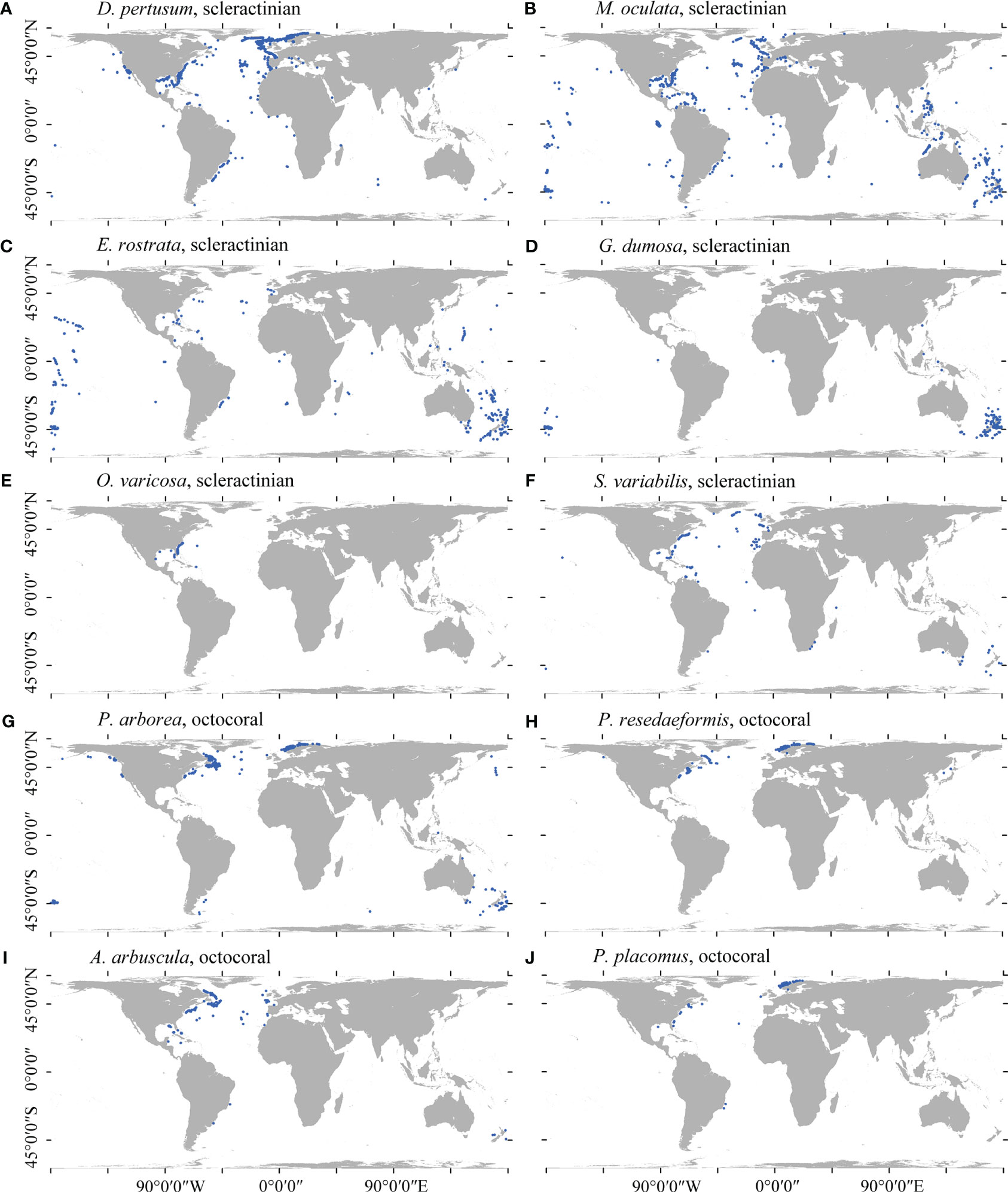
Figure 1 Spatial distribution of the cleaned presence records for each of the 10 cold-water coral species in this study. (A) D pertusum, (B) M. oculata, (C) E rostrata, (D) G dumosa, (E) O. varicosa, (F) S. variabilis, (G) P. arborea, (H) P. resedaeformis, (I) A arbuscula, and (J) P. placomus.
The seabed environmental data used in this study were built around a publicly available high-resolution global bathymetric data product obtained from the General Bathymetric Chart of the Ocean. The 2022 grid was assembled from multiple sources, such as acoustic soundings, multibeam bathymetry, and satellite altimetry (GEBCO Compilation Group, 2022). For subsequent variable creation and analysis, the bathymetric grid, originally a 15 arc-second grid, was projected into the NSIDC Equal-Area Scalable Earth (EASE) Grid (EASE-Grid 2.0 Global, EPSG: 6933) with a cell size of 500 m. The projected bathymetric grid was used to calculate seven terrain variables, namely slope, curvature, terrain ruggedness index (TRI), topographic position index (TPI) and roughness using an analysis window size of 3 × 3 cells, and bathymetric position index (BPI) with analysis window sizes of 3 × 3 and 9 × 9 cells (Wilson et al., 2007). Slope, curvature, and BPI were calculated using ArcGIS Pro v2.5. TRI, TPI, and roughness were calculated using QGIS v3.28.2.
Seafloor conditions for 11 variables were obtained via a trilinear interpolation approach whereby each cell of the bathymetric data layer was used to calculate conditions from regularly structured environmental data available at standard depth levels (Table 1). Two main inputs were used, World Ocean Atlas 2018 (102 depth layers; mean of all available years for oxygen and nutrient variables, and mean of data collected between 1955 and 2017 for temperature and salinity) (Garcia et al., 2018a; Garcia et al., 2018b; Locarnini et al., 2018; Zweng et al., 2018) and GLODAP V2. 2016b (Global Ocean Data Analysis Project; 33 depth layers; mean of data collected between 1972 and 2013) (Lauvset et al., 2016). Each depth layer was first extracted to a horizontal depth layer of points and resampled to a projected continuous global raster using Natural Neighbor interpolation using the arcpy Python package from ArcGIS Pro v3.1. Where depth cells fell below the maximum depth of the structured environmental grid, we extrapolated the deepest environmental layer to exceed the maximum depth by 1 m. These layers were then used to create an array of eight points centered around each depth cell from which the environmental condition was estimated using the regular grid interpolator function (trilinear interpolation) from the Python package scipy v1.6.2 (Virtanen et al., 2020). This approach represents improvements over earlier global studies that utilized alternative variable up-scaling approaches (e.g., Davies and Guinotte, 2011), by providing a more accurate interpolation of structured environmental data, and enables an increase in resolution that is commensurate with the input bathymetric grid (Table 1).
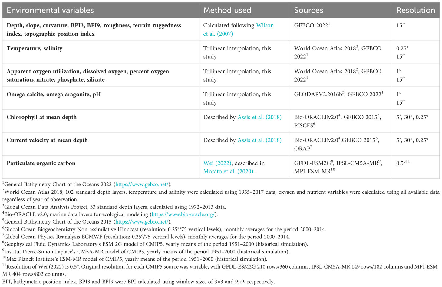
Table 1 Sources and original resolution for environmental variables created in this study.
Each interpolated seafloor environmental layer was validated where possible using biogeochemical data obtained from GLODAP, an aggregated and quality controlled water bottle dataset of ocean surface to bottom conditions (Lauvset et al., 2022). Records of bottom values were extracted from GLODAP v2-2022 using Ocean Data View v5.6.3 (Schlitzer, 2023). Estimates of omega aragonite and omega calcite from the GLODAP v2-2022 dataset were calculated from extracted parameter records using the Seacarb algorithm (Gattuso et al., 2022). Linear least squares regression was used to estimate the relationship between the extracted bottle data from GLODAP v2-2022 and the trilinearly interpolated bottom layer for each variable. In addition, a visual spatial validation was conducted by creating a polygon grid with cells sized 500 × 500 km that extended across the model domain (Supplementary Figure 2). Differences between the observed GLODAP data and the predicted trilinear value were expressed as root mean square error (RMSE) on a cell-by-cell basis. For visualization purposes, RMSE was scaled using the standard deviation of all observed GLODAP points for that variable.
Three additional environmental variables of ocean floor conditions were also obtained from two datasets, including the Bio-ORACLE v2.0 dataset (Assis et al., 2018) and Wei (2022) (Table 1), projected to EASE-Grid 2.0 Global and resampled to 500m resolution using bilinear interpolation using Python v3.8 and GDAL v3.2.3. This validation showed significant correlation between modeled environmental variables and field observations (Pearson’s correlation coefficient r > 0.93), with the exception of Chlorophyll a (r = 0.56) obtained from Bio-ORACLE, as reported by Assis et al. (2018). Particulate organic carbon obtained from Wei (2022) was found to be strongly correlated with field observations from a previous study (Lutz et al., 2007) in the North Atlantic with r = 0.91 (Morato et al., 2020).
Strongly correlated environmental factors may impede model performance and their ultimate interpretation in SDMs (Huang et al., 2011). In this study, variance inflation factor (VIF) was used to analyze the correlation among environmental variables, with a high VIF value indicating a high degree of co-linearity between a variable and all remaining variables (Yesson et al., 2015; Yesson et al., 2017; Khosravifard et al., 2020). In this study, the VIF was calculated iteratively with the highest VIF variable removed each time, until the VIF value of each retained variable was less than 10, indicating low correlation, using the R package HH v3.1-49 (Heiberger, 2022). Fully automating any procedure to remove highly correlated variables can result in the removal of ecologically relevant factors (Davies and Guinotte, 2011; Yesson et al., 2017; Tong et al., 2022). Therefore, the variables slope, percent oxygen saturation and one of omega aragonite or omega calcite dependent upon the skeletal structure of each species were always retained, along with other environmental variables that had VIF <10 (excluding other oxygen parameters were all strongly correlated with Spearman correlation coefficients ≥ 0.94) (Table 2) (Guinotte et al., 2006a; Sundahl et al., 2020; Matos et al., 2021). Specifically, omega aragonite and omega calcite were used for predictions of Scleractinia and Octocorallia, respectively.
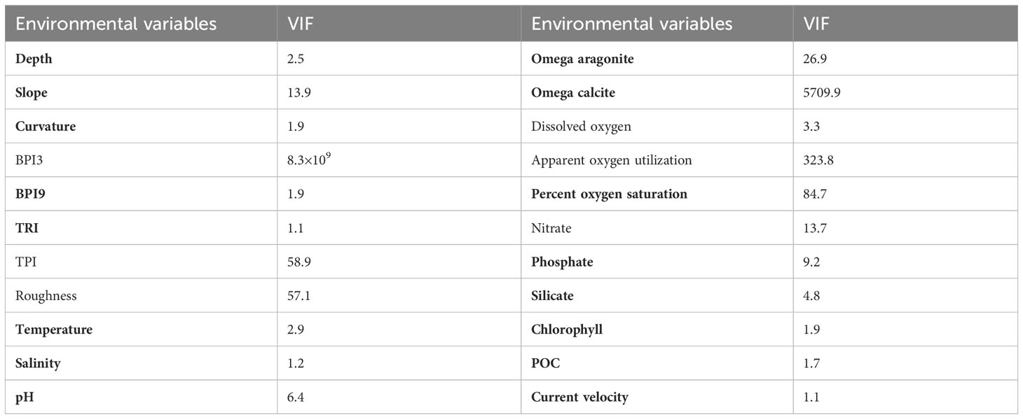
Table 2 Variable inflation factors (VIF) calculated for each environmental variable, with the variables utilized in predictions highlighted in bold.
Each species distribution modeling method has its own strengths and weaknesses (Liu et al., 2016; Grimmett et al., 2020); ensemble modeling integrates the outputs of multiple species distribution models in a prediction to reduce reliance on a single model or distribution assumption (Robert et al., 2016; Valavi et al., 2022). In this study, we used two machine learning methods, generalized boosting modeling (GBM, also described as boosted regression trees; BRT) (Ridgeway, 1999) and random forests (RF) (Breiman, 2001). GBM employs a boosting algorithm to iteratively call a regression tree algorithm in order to construct a combination of trees (Ridgeway, 1999). GBM iteratively modifies the modeled regression trees to improve their fit to the data (Friedman, 2001) and is often among the best-performing predictive modeling approaches (Elith et al., 2006; Valavi et al., 2022). RF constructs a number of regression trees and then averages them (Breiman, 2001), with the trees growing based on multiple training data subsets that are established via a bagging technique to avoid tree correlation (Rodriguez-Galiano et al., 2015). Both GBM and RF are commonly used for predicting species habitat suitability and often demonstrate high performances when used in ensemble modeling approaches. The R package biomod2 v4.2-1 was used to build the species distribution models (Thuiller et al., 2022).
To generate an individual model for each species, models were run in a block cross-validation approach to reduce the influence of spatial autocorrelation that arises due to geographically concentrated sampling activity (Valavi et al., 2019; Winship et al., 2020; Valavi et al., 2022). The presence records of each species were evenly divided into five folds based on longitude, with each fold containing one-fifth of the total amount of records, and the pseudo-absence points divided accordingly. For each replicate, four of the five folds were used for model training, with one fold being withheld from model training and used for model validation. AUC [area under the ROC (receiver operator characteristic) curve], TSS (true skill statistic), sensitivity, specificity, and Continuous Boyce Index (Hirzel et al., 2006) were calculated to evaluate the performances of the models.
The ensemble model prediction that combined the GBM and RF models for each species was calculated as the weighted average of each individual model output, utilizing the model performance statistic AUC for each run as weighting and only including predicted models that had an AUC greater than 0.8. The standard deviation of these predicted maps with AUC greater than 0.8 for each species was calculated to provide the information of model uncertainty to support the predictions. Binary habitat suitability maps for each species were calculated using the threshold value calculated from the maximum sensitivity and specificity for each species, setting habitat suitability values below the threshold to zero (unsuitable), and those above to one (suitable). The binary projection for each species was further limited to depth shallower than the maximum depth of the corresponding species’ presence. These calculations were performed using ArcGIS Pro v2.5.
The ordination method principal component analysis (PCA) was used to investigate the fundamental ecological niches of cold-water coral species. The PCA was calibrated on the entire environmental space of the global ocean (PCA-env) by utilizing values of environmental variables associated with 200,000 randomly selected background points (representing the bottom environmental condition of global ocean) to convert from geographic space to environmental space and create a grid consisting of 100 × 100 pixels (Broennimann et al., 2012; Di Cola et al., 2017). Kernel smoothers were used to quantify densities of species occurrence in the gridded environmental space, delimited by axes with the 100 × 100 pixels, to create an occurrence density grid for each species (Broennimann et al., 2012). Schoener’s D metric (Schoener, 1970) was used to estimate niche overlap of species pairs and to test niche similarity and equivalency by determining whether environmental niches of a species pair were more similar than expected by chance, using occurrence density grids of the species pair (Warren et al., 2008; Barbosa et al., 2020). Niche breadth was calculated as the proportion of the available environmental conditions delimited by the axes (100 × 100 cells) occupied by species in the PCA-env, representing the percentage of available conditions inhabited by the species. The contribution of the environmental variables to the PCA was presented as eigen vectors in the correlation circle plot (Di Cola et al., 2017). The R package Ecospat v3.4 was utilized for the analyses (Broenniman et al., 2022).
In total, 7,496 presence records, namely, 3,069 for D. pertusum, 1,412 for M. oculata, 574 for E. rostrata, 563 for G. dumosa, 148 for O. varicosa, 226 for S. variabilis, 767 for P. arborea, 362 for P. resedaeformis, 203 for A. arbuscula, and 172 for P. placomus, were retained for analyses (Figure 1).
Validation of each seafloor environmental variable developed using the trilinear interpolation approach showed significant correlations between the constructed environmental variables and water bottle data (R2 between 0.786 and 0.987; Figure 2). Spatial validation showed that most variables had low scaled RMSE throughout the global ocean, with higher error values on continental shelf margins where depths change rapidly (Supplementary Figure 2). Temperature and salinity, with higher native horizontal spatial resolutions (0.25°), performed better than variables with native resolutions of 1°, although some areas of mid to high RMSE were observed on continental shelves and margins, particularly in the North Atlantic (Supplementary Figure 2). Nevertheless, these variables demonstrated strong correlations with GLODAP data, with R2 values of 0.930 and 0.877, respectively (Figure 2). Silicate, nitrate, phosphate, apparent oxygen utilization, and dissolved oxygen, with a native horizontal resolution of 1°, showed greater variation in RMSE, but were among the top-ranked variables with strong correlations with GLODAP data (Figure 2 and Supplementary Figure 2). Carbonate variables, omega aragonite and omega calcite, had a larger degree of error, largely in the Atlantic Ocean (Supplementary Figure 2), and performed less well in comparison with GLODAP data in the regression analyses (Figure 2).
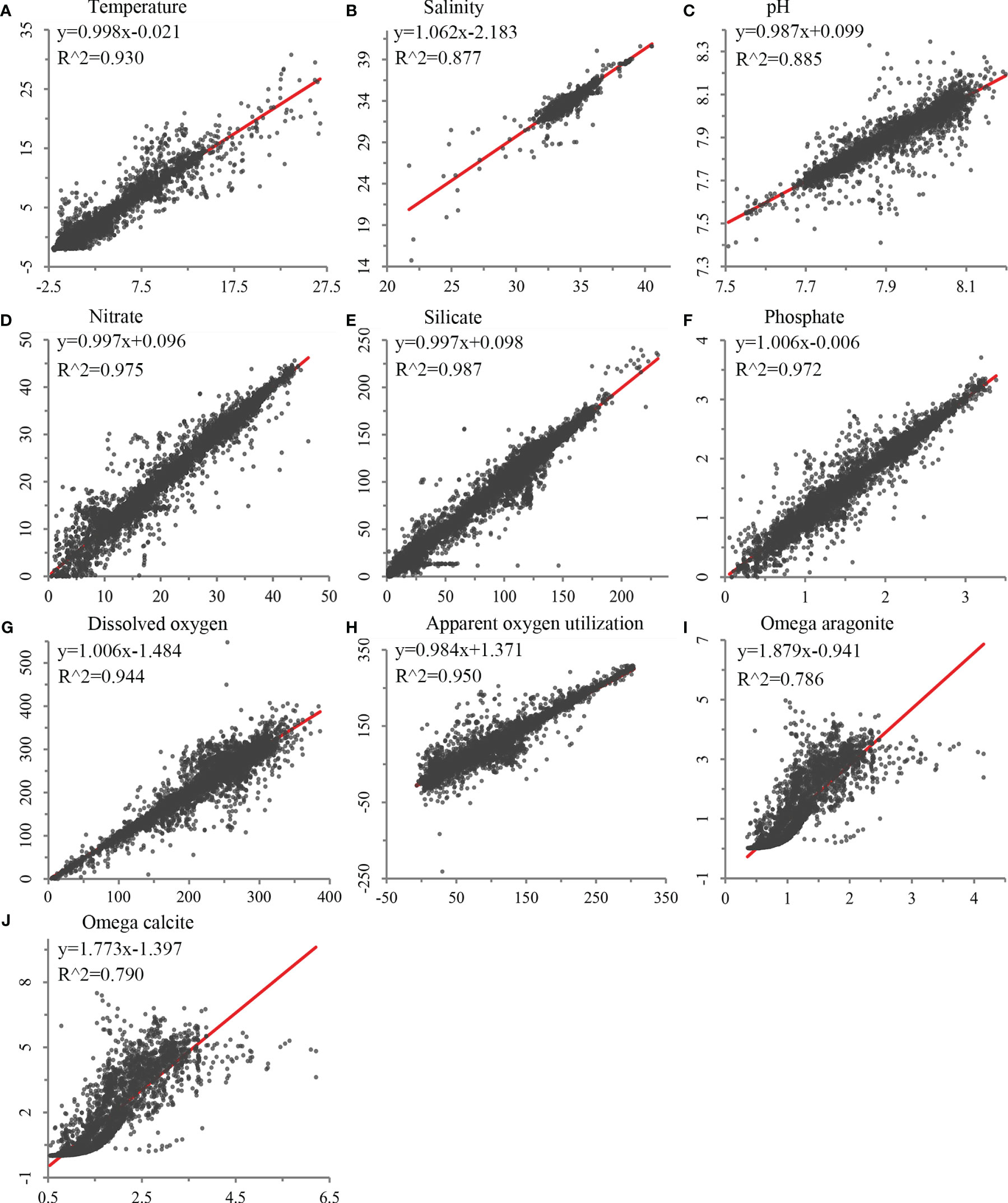
Figure 2 Validation of environmental variables built in this study against field sampling data using least squares regression, using bottle data for (A) temperature (N = 27,983), (B) salinity (N = 27,556), (C) pH (N = 9,559), (D) nitrate (N = 21,453), (E) silicate (N = 21,799), (F) phosphate (N = 20,158), (G) dissolved oxygen (N = 24,782), (H) apparent oxygen utilization (N = 24,123), and (I) omega aragonite and (J) omega calcite (N = 9,559).
All 10 cold-water coral species were observed predominantly in waters shallower than −2,000 m water depth that had higher mean temperature, pH, and particulate organic carbon than the global means for these variables (Figures 3, 4). In addition, these species were found in areas that were mostly saturated in aragonite and calcite but had a lower mean silicate concentration than the global oceans. Oculina varicosa was found in areas that had the greatest differences in environmental conditions compared to the other nine species. On average, O. varicosa occured in much shallower (mean water depth −85.2 m), warmer (23.9°C) and saltier (36.3) waters, with higher means for omega aragonite (saturation state 3.6), percent oxygen saturation (95.3%), pH (8.07), and chlorophyll (0.25 mg/m3) compared to other species. Mean phosphate (0.19 μmol/kg) and mean silicate (2.2 μmol/kg), in contrast, were lower than mean values for other species locations (Figure 4). Solenosmilia variabilis was averagely found in deeper food limited waters that had higher relief and current velocity than other species (mean depth −1,190 m, mean terrain ruggedness index 230.8 m, mean chlorophyll 0.009 mg/m3, and mean current velocity 0.14 m/s). In contrast, M. oculata and E. rostrata exhibited a more dispersed distribution across broad ranges of depth, temperature, omega aragonite, oxygen saturation, pH, phosphate, and silicate. Desmophyllum pertusum, G. dumosa, P. arborea, P. resedaeformis, and P. placomus were found predominantly in a relatively narrow range of environmental conditions, especially for depth and silicate (Figures 3, 4). Acanella arbuscula was found across a wide depth range (−24 m to −4,814 m, with mean depth −1,077 m) and at the lowest mean temperature 4.3°C, compared to the other species (Figure 3).

Figure 3 The distribution profiles of eight environmental variables are shown for each of the 10 cold-water coral species (shown in dark gray) in contrast to the global background (shown in light gray in the first column of each panel). The environmental variables examined include (A) depth, (B) TRI, (C) temperature, (D) salinity, (E) omega aragonite, (F) omega calcite, (G) percent oxygen saturation, and (H) pH. Black lines represent mean values. Species names were abbreviated for clarity: DP, D. pertusum; MO, M. oculata; ER, E. rostrata; GD, G. dumosa; OV, O. varicosa; SV, S. variabilis; PA, P. arborea; PR, P. resedaeformis; AA, A. arbuscula; and PP, P. placomus.
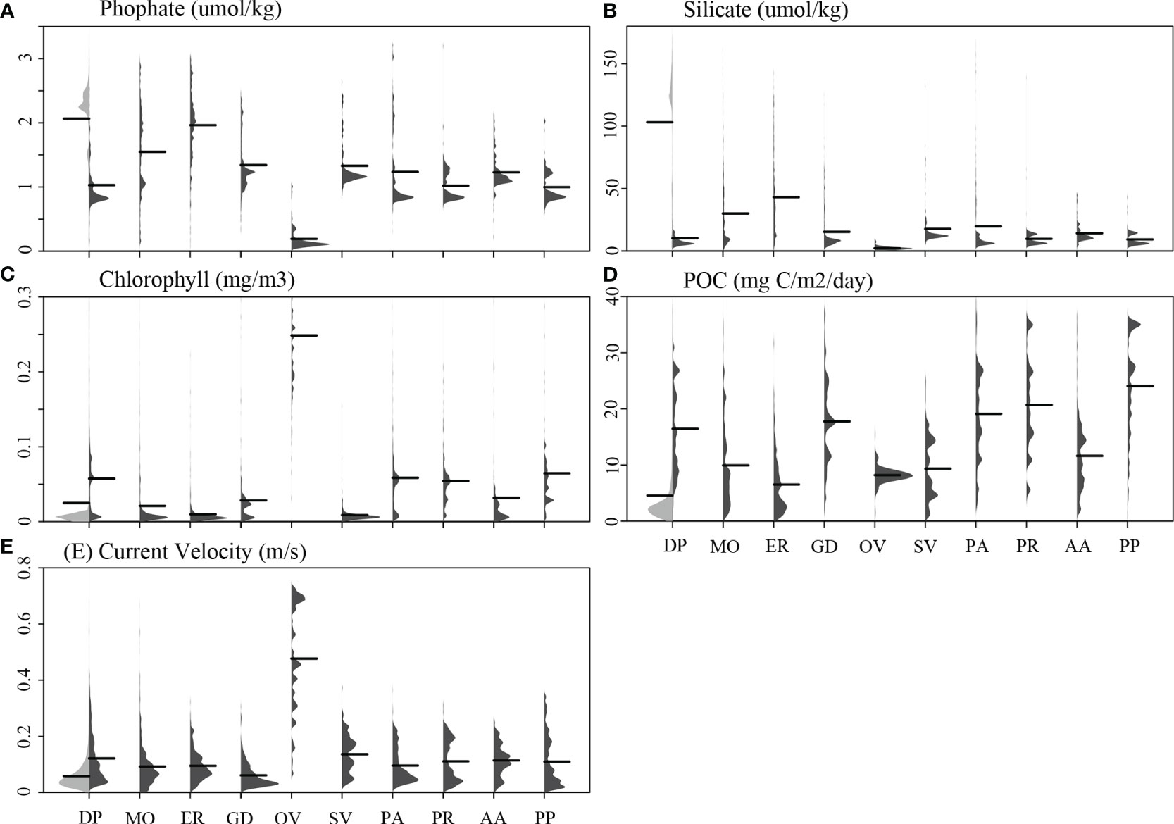
Figure 4 The distribution profiles of five environmental variables are shown for each of the 10 cold-water coral species (shown in dark gray) in contrast to the global background (shown in light gray in the first column of each panel). The environmental variables examined include (A) phosphate, (B) silicate, (C) chlorophyll, (D) POC, and (E) current velocity. Black lines represent mean values. Species names were abbreviated for clarity: DP, D. pertusum; MO, M. oculata; ER, E. rostrata; GD, G. dumosa; OV, O. varicosa; SV, S. variabilis; PA, P. arborea; PR, P. resedaeformis; AA, A. arbuscula; PP, P. placomus.
The strongest contributors, assessed by the mean variable importance score from the fivefold block cross-validation predictions for each species, were largely temperature and depth, but salinity was also observed to be a strong contributor for several species followed by variables such as TRI, chlorophyll, carbonate saturation state, current velocity, and oxygen saturation (Table 3). For 5 of the 10 species, the two modeling approaches agreed as to the top contributing variables, but some differences in the top three variables selected were present (Table 3). Temperature, salinity, and TRI were most important in predictions for D. pertusum, while depth, temperature, and percent oxygen saturation were most important in predictions for M. oculata, as well as depth, salinity, and TRI for E. rostrata, depth, chlorophyll, and temperature for P. arborea and P. resedaeformis, and depth, TRI, and temperature for P. placomus. TRI and temperature were most important in predictions for S. variabilis, while salinity and temperature were most important in predictions for G. dumosa, as well as salinity, chlorophyll, and current velocity to O. varicosa, and omega calcite, salinity, and temperature to A. arbuscula (Table 3).
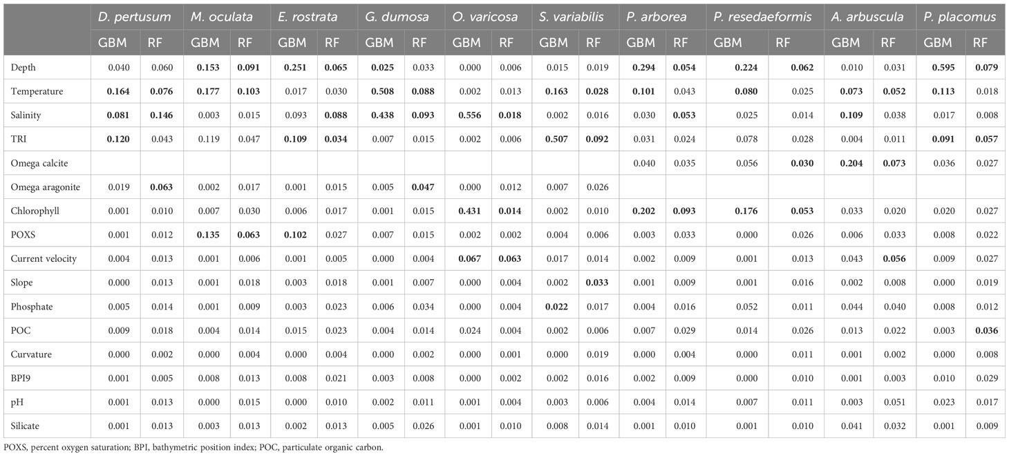
Table 3 Mean variable importance of each environmental variable in models constructed using fivefold block cross-validation, with the top three highest scoring variables highlighted in bold for each model and species combination.
In this study, both the GBM and RF approaches performed well, with mean AUC values for GBM predictions ranging from 0.871 to 0.984 (standard deviation: 0.015 to 0.115). Similarly, RF models performed well with mean AUC values of 0.87 to 0.993 (standard deviation: 0.007 to 0.115) for all species (Table 4). The mean TSS value for each species greater than 0.655 showed good agreement between predicted habitat suitability and the known presence/pseudo-absence of the validation dataset. The mean sensitivity was greater than the corresponding mean specificity for most species, including 7 out of 10 species in GBM predictions and 6 out of 10 species in RF predictions, indicating that the models had a higher ability to correctly identify the presence of suitable habitat compared to the pseudo-absence points. The Continuous Boyce Index of these model runs was variable, but with the mean value ≥0.616 suggesting a positive correlation between the model’s predictions and the observed presences (Table 4). Predicted habitat suitability for each cold-water coral species varied substantially by geographic region around the world (Figures 5–8), with the most suitable habitat found on continental shelves and margins in the North Atlantic, West and South Pacific, the Gulf of Mexico, the Caribbean Sea, the Mediterranean Sea, the Red Sea, and the seamounts and steep slopes of oceanic islands.
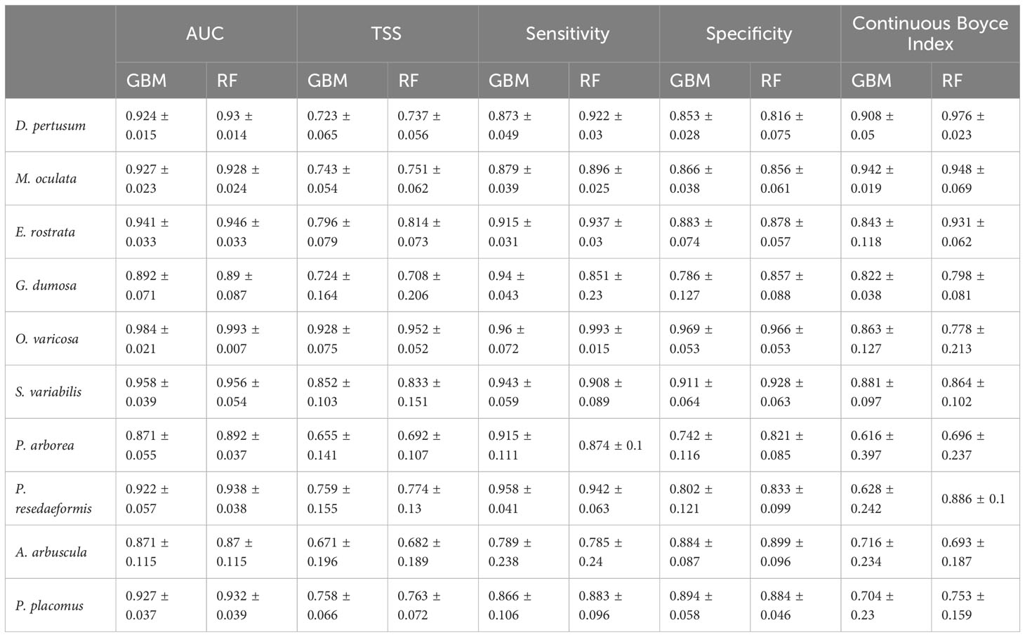
Table 4 Model evaluation results, including mean and standard deviation of AUC, TSS, sensitivity, specificity and Continuous Boyce Index values from the fivefold block cross-validation of predictions for each individual species using the two modeling approaches, GBM and RF.
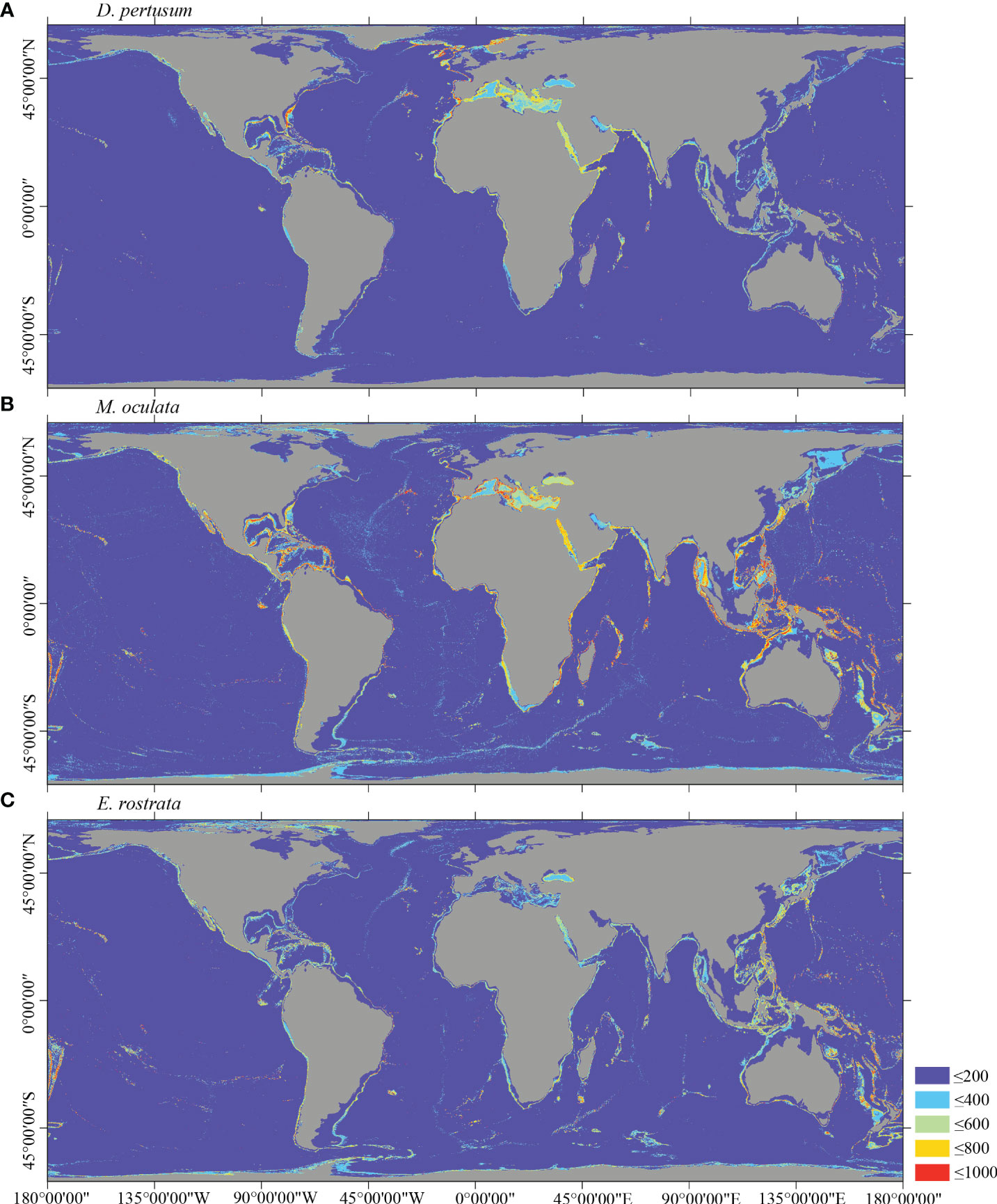
Figure 5 Predicted habitat suitability (0–1,000) at the global scale for cold-water corals (A) D pertusum, (B) M. oculata, and (C) E rostrata using ensemble modeling. Warmer color shows areas of high habitat suitability.
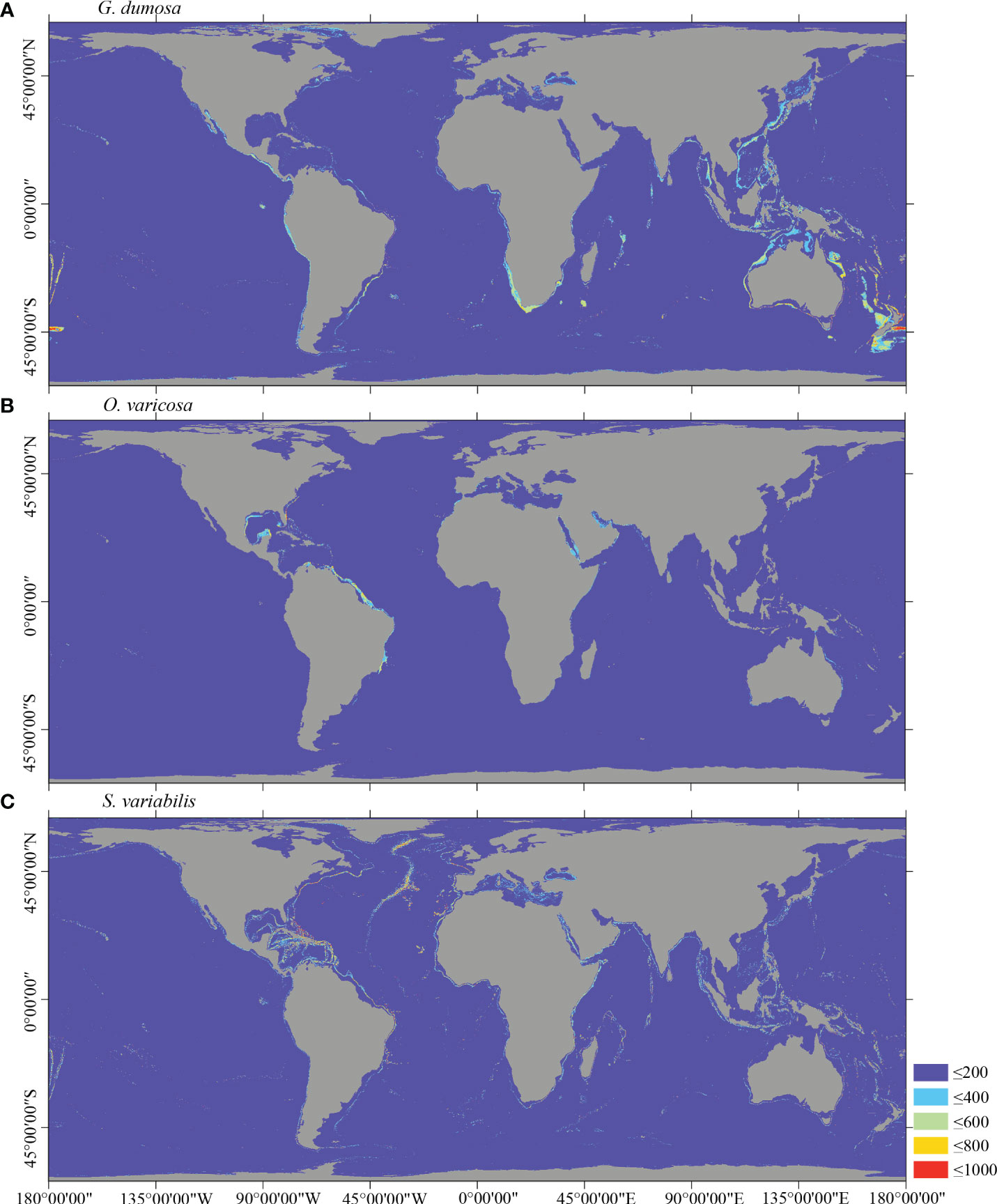
Figure 6 Predicted habitat suitability (0–1,000) at the global scale for cold-water corals (A) G dumosa, (B) O. varicosa, and (C) S. variabilis using ensemble modeling. Warmer colors show areas of high habitat suitability.

Figure 7 Predicted habitat suitability (0–1,000) at the global scale for cold-water corals (A) P. arborea and (B) P. resedaeformis using ensemble modeling. Warmer colors show areas of high habitat suitability.
Several specific regional differences were observed for each species. Desmophyllum pertusum, for example, was predicted predominantly in the NE Atlantic, around the Mediterranean Sea, and on the continental margin off the SE USA (Figure 5A and Supplementary Figure 3A). In comparison, the predicted suitable habitat for M. oculata and E. rostrata was less prevalent in the North Atlantic and more so in the West and South Pacific and the Red Sea, around the Mediterranean Sea, the Gulf of Mexico, and the Caribbean Sea (Figures 5B, C and Supplementary Figures 3B, C). The predicted habitat suitability for each species differed substantially in terms of areal extent, with M. oculata having the greatest potential range and O. varicosa having the smallest, being largely restricted to some areas off the SE USA and regions off South America (Figures 5B, 6B and Supplementary Figures 3B, 4B). Suitable habitat for G. dumosa was predicted in the West and South Pacific, particularly in the waters surrounding New Zealand, as well as along the continental margin off SW Africa (Figure 6A and Supplementary Figure 4A). Solenosmilia variabilis was predicted predominantly in the North Atlantic, around the Caribbean Sea and the Gulf of Mexico, particularly along the Mid-Atlantic Ridge, as well as in the South Pacific (Figure 6C and Supplementary Figure 4C). The majority of suitable habitat for P. arborea was found on the continental shelves of the North Atlantic and the North Pacific, off the southeastern coast of South America, southeastern New Zealand, and on seamounts (Figure 7A and Supplementary Figure 5A). In contrast to P. arborea, P. resedaeformis and P. placomus were predicted to have a more restricted suitable habitat, mainly in the North Atlantic (Figures 7B, 8B and Supplementary Figures 5B, 6B). Acanella arbuscula was predicted to occur predominantly on the continental shelf margin of the West Atlantic (Figure 8A and Supplementary Figure 6A). The standard deviation of predicted maps for each species showed more areas of higher uncertainty for G. dumosa predictions than those for other species (Supplementary Figure 7).
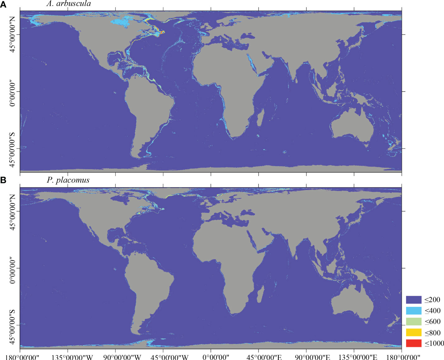
Figure 8 Predicted habitat suitability (0–1,000) at the global scale for cold-water corals (A) A arbuscula and (B) P. placomus using ensemble modeling. Warmer colors show areas of high habitat suitability.
Among the environmental variables utilized in predictions, the terrain variables slope, curvature, and BPI rarely were important in predictions for the 10 species and, therefore, were excluded from further ecological niche analysis. Twelve environmental variables (depth, TRI, temperature, salinity, pH, omega aragonite, phosphate, silicate, percent oxygen saturation, chlorophyll, particulate organic carbon, and current velocity) were used in the ecological niche analysis for each species (Figure 9).
The correlation circle of PCA-env describes the contribution of each variable to the global environmental conditions captured by the first two principal components, which can help to further identify and understand the environmental variables that shape ecological niches. It shows that omega aragonite, pH, and temperature mainly contribute to the first principal component axis (PC1), and salinity and TRI mainly contribute to the second principal component axis (PC2), while depth, percent oxygen saturation, current velocity, chlorophyll, particulate organic carbon, phosphate and silicate contribute to both PC1 and PC2 axes (Figure 9M). The two principal components explained 46.46% and 11.94% of the information regarding the global environmental conditions, respectively (Figure 9M). The ecological niche breadth of each species significantly varied, with M. oculata having the broadest niche, followed by E. rostrata (Figures 9B, C). The location of niche density center of O. varicosa was quite different to niche density centers of nine other species, with limited overlap (Figure 9E; Table 5). The niche density centers of S. variabilis and A. arbuscula were close, with their niches showing high level of overlap (Figures 9F, I). The niche density centers of D. pertusum, G. dumosa, P. arborea, P. resedaeformis, and P. placomus were close, showing high level degree of niche overlap between each pair of these species, particularly for P. resedaeformis and D. pertusum, and P. resedaeformis and P. placomus (Figures 9A, D, G, H, J; Table 5). The niche similarity for each pair of species was all rejected with p > 0.05, except between D. pertusum and P. resedaeformis, between D. pertusum and P. placomus, and between P. resedaeformis and P. placomus. There were certain degree of niche overlap between Scleractinia and Octocorallia (Figures 9K, L; Table 5). No evidence of niche equivalency was found (Table 5).
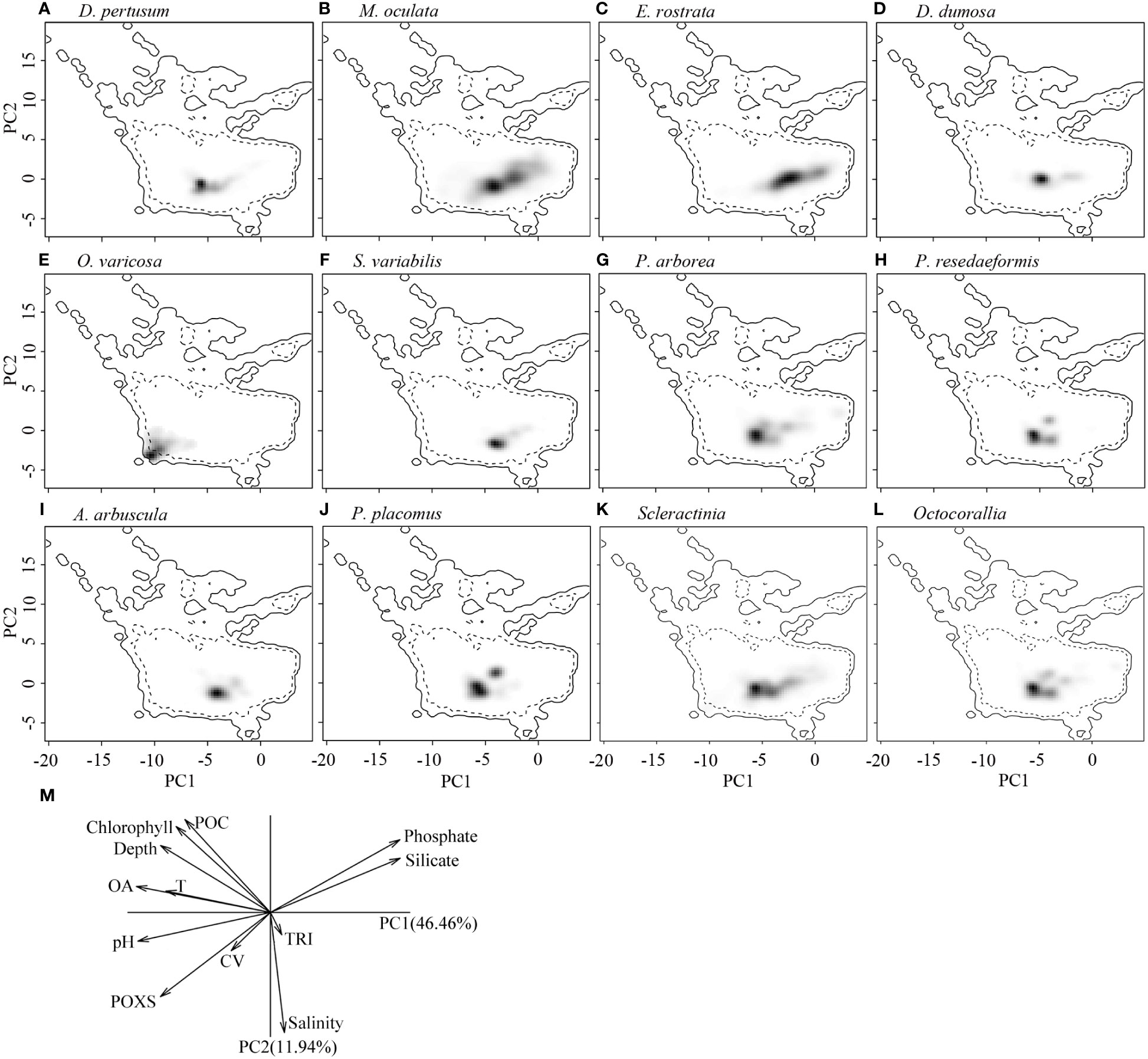
Figure 9 Estimated ecological niches of the 10 cold-water coral species, Scleractina, and Octocorallia by principal component analysis, with the environmental space determined by the axes of PC1 and PC2 (A–L). The gray to black shading represents the kernel density of species presence, with black showing the highest density. The solid lines represent the 100% of available environmental conditions within the global ocean environmental data, while dashed lines represent 50% of available environmental conditions. (M) shows the contribution of each variable to the two principal components in ecological niche analysis using principal component analysis, with omega aragonite used to express water carbonate conditions. POXS, percentage oxygen saturation; OA, omega aragonite; POC, particulate organic carbon; T, temperature; TRI, terrain ruggedness index; CV, current velocity.
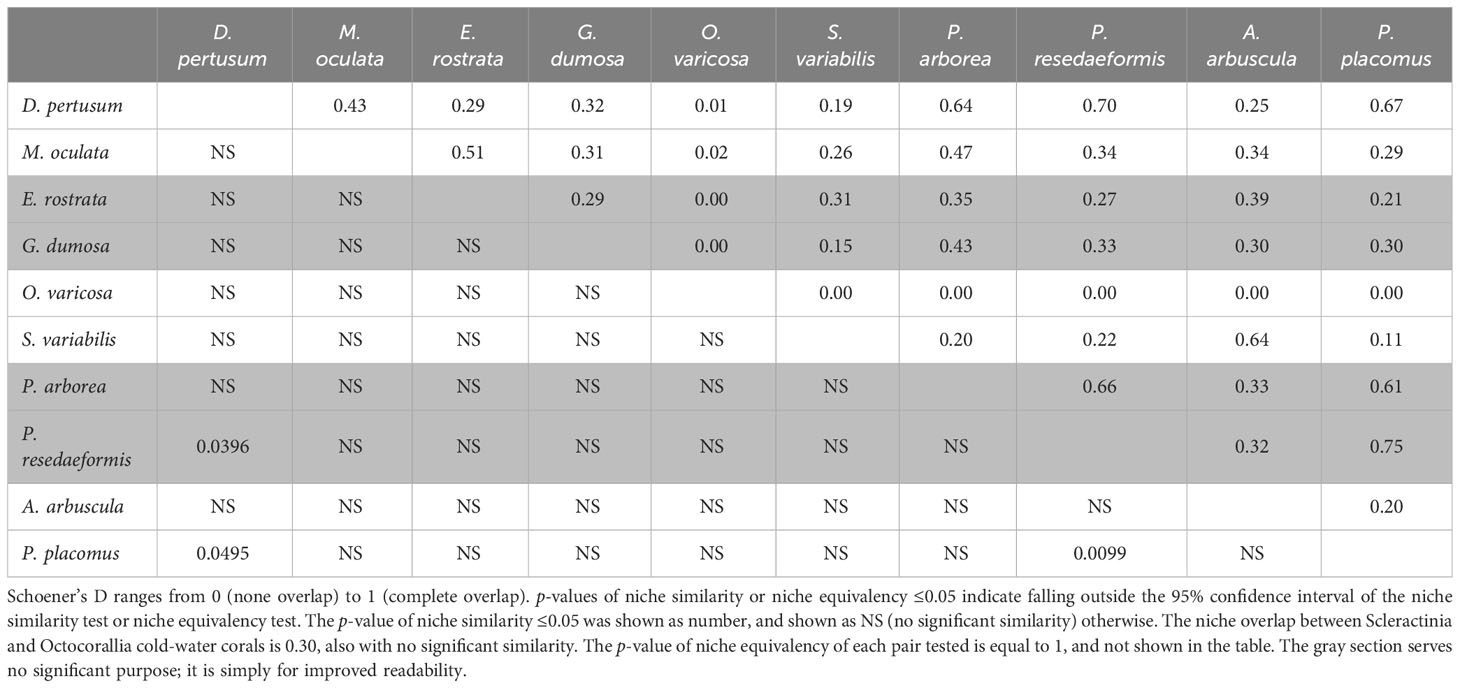
Table 5 Niche comparison for each pair of the 10 species using Schoener’s D, with the upper triangle representing niche overlap (D) and the lower triangle representing the p-value of niche similarity.
In this study, using a high-resolution bathymetric grid, updated environmental variables, and presence records, new predictions of the global distribution of 10 cold-water coral species are developed and have reached a high level of resolution, allowing for additional analyses into the species niches of these enigmatic cold-water coral habitats.
The current study represents a substantial improvement in the resolution and geographic extent of distribution predictions for cold-water corals in the deep ocean (Davies and Guinotte, 2011; Yesson et al., 2012; Yesson et al., 2017; Tong et al., 2022). The resolution of the bathymetric dataset is now approximately 500 m (compared with the previous ~1 km), while coverage of high-quality acoustic measurements now covers 24.7% of the global seafloor (calculated using the GEBCO Type Identifier Grid) (Supplementary Figure 8) (GEBCO Compilation Group, 2022). These high-quality measurements were predominantly located in the North Atlantic and in areas of the East, West, and South Pacific, particularly surrounding the continental margins and large oceanic islands, generally consistent with currently known locations of cold-water corals (Supplementary Figure 8; Figure 1). However, the majority of the bathymetry layer was generated from indirect methods that are characterized by low resolution, such as satellite-derived gravity measurements. These data are further interpolated and lead to the generation of a relatively smooth surface that largely misses a number of seafloor features such as seamounts and canyons below a certain size (Kvile et al., 2014; Yesson et al., 2021). Given that depth remains a critically important variable in assessing global cold-water coral distribution, and that terrain variables such as TRI have emerged as increasingly important in global-scale models, ongoing efforts to improve global bathymetric data will continue to enhance distribution models generated at regional to global scales. GEBCO’s Seabed 2030 project is one such initiative, which aims for complete global coverage by 2030, and will serve to improve our ability to predict species distributions (Mayer et al., 2018; Wolfl et al., 2019), particularly those in under-surveyed environments.
The quality of the underlying environment layers has also improved since the earlier studies, as evidenced by the higher regression R2 values for five out of six variables built in this study compared to the validation results of the six variables in the widely used Bio-ORACLE v2.0 dataset, including salinity, nitrate, phosphate, silicate, and dissolved oxygen, only with the exception of temperature (Assis et al., 2018). Previous studies used inverse distance weighting interpolation and a resampling methodology utilizing a bathymetric grid to downscale global environmental variables obtained from NOAA’s World Ocean Atlas (Boyer et al., 2005; Garcia et al., 2006a; Garcia et al., 2006b), which was available at a source horizontal resolution of 0.25° for temperature and salinity, and 1° for other variables (Davies and Guinotte, 2011; Yesson et al., 2017). Vertical resolution has been significantly extended, increasing from the 33 World Ocean Atlas depth layers used in Davies and Guinotte (2011) to the 102 depth layers that are used in this study (Garcia et al., 2018a; Garcia et al., 2018b; Locarnini et al., 2018). The increase in vertical resolution and the use of a new interpolation technique (trilinear interpolation) provide a substantial improvement in the estimations of seafloor condition, particularly in depths shallower than or equal to 2,000 m, where the majority of coral species are found, and lead to finer and more constrained predictions (Figure 10).
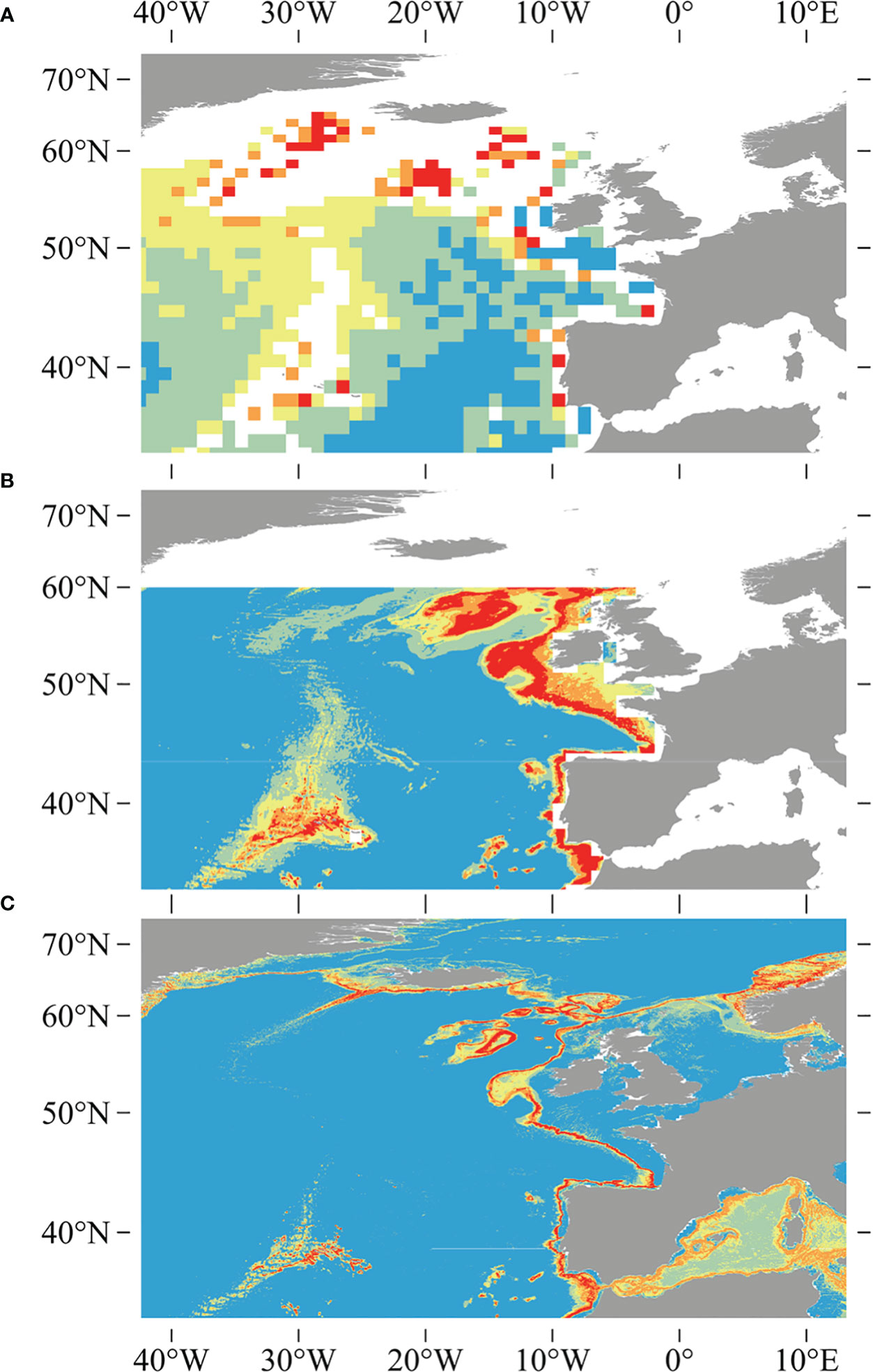
Figure 10 Comparisons between earlier studies of outputs for D pertusum, including (A) the global model created using ecological niche factor analysis in Davies et al. (2008), (B) the model created using the Maxent modeling approach and 1,000-m-resolution bathymetry in Davies and Guinotte (2011), and (C) the model generated using 500-m-resolution bathymetry and an ensemble modeling approach in this study. Note reduction in over-prediction and increase in resolution of this study relative to earlier studies.
The species pool in this study was widened by adding four common gorgonians, which have not been modeled in a consistent fashion before in a global study, enabling global assessment of the niche of cold-water coral species. The number of presence records for most species used in this study was significantly larger than in previous global modeling studies for cold-water corals (Davies and Guinotte, 2011). Compared to earlier studies, these data represent an increase in data density for most species, including a minimum of 356% (D. pertusum), 239% (M. oculata), 267% (E. rostrata), and 245% (G. dumosa), while S. variabilis has decreased to 59% of its earlier quantity (Davies et al., 2008; Davies and Guinotte, 2011). The improved grid cell size of 500 m also played a role in increasing the total number of presence records used in predictions as it allowed for the retention of a single record within a grid cell. However, strict limitations of positional and depth accuracy (500 m horizontal or 50 m vertical) were used to constrain to a subset of high-quality presences that have additional metadata, excluding a number of presence records that were utilized in earlier studies (Davies and Guinotte, 2011). The significant increase of presences can improve the model performances (Grimmett et al., 2020), but particular attention should be focused on increasing the taxonomic quality, accuracy, and delivery of metadata to further ensure that modeling efforts in the deep ocean are valid and reach sufficient standards as outlined by Araújo et al. (2019).
Comparing our models with large-scale predictions, it is evident that our models have significantly improved compared to previous efforts (e.g., Figure 10). This improvement can be attributed partly to the inclusion of environmental variables of higher horizontal and vertical resolution in our models than previous studies (Connor et al., 2018). Nevertheless, it is important to note that despite these advancements, our models still tend to over-predict when compared to predictions at the local and sub-regional scale that use additional high-resolution environmental variables. For example, extensive suitable habitat for D. pertusum, P. arborea, and P. resedaeformis predicted on the Norwegian margin was broadly similar to previous high-resolution regional prediction, but over-predicted compared to models incorporating seafloor substratum and marine landscape metrics (Sundahl et al., 2020). In the Mediterranean Sea, high suitable habitat for D. pertusum was predicted predominantly along the upper slope and submarine canyons of the Western and Central margins, which is consistent with the findings of Matos et al. (2021). However, there is still an issue of over-prediction, particularly in the northeast section of the Mediterranean Sea. Similarly, in New Zealand waters, the pattern of significantly higher predicted habitat suitability on Chatham Rise compared to Campbell Plateau for G. dumosa aligns with the regional prediction that incorporates higher-resolution environmental variables, such as tidal current speed at a resolution of 1 km (Stephenson et al., 2021a). Nonetheless, over-prediction remains a concern. Habitat suitability models built at smaller spatial scales likely provide more accurate predictions than those generated at the global scale, as they can integrate higher-quality environmental data that may be available at finer spatial scales.
Sampling bias can introduce spatial autocorrelation into species distribution models (de Oliveira et al., 2014). Autocorrelation between training observations and testing observations violates the classical assumption of identically and independently distributed data commonly used in machine learning (Beigaite et al., 2022), which may induce autocorrelated model residuals, introducing biases in model parameter estimates and over-optimistic assessment of model predictive power, particularly in the case of highly clustered sampling (Ploton et al., 2020). In this study, sampling bias is evident, as cold-water coral presence records are abundant in the North Atlantic and South Pacific, but scarce in the North Pacific and Indian Ocean. Various spatial cross-validation strategies have been developed aiming to create independence between cross-validation folds (Roberts et al., 2017; Beigaite et al., 2022; Valavi et al., 2023). However, Wadoux et al. (2021) argue that spatial cross-validation leads to under-representation of environmental conditions similar to those at validation locations, and is likely to be over-pessimistic if there are significant differences in environmental conditions between validation and calibration folds (Wadoux et al., 2021). In this study, the predictive performance for most of the species (8 out of 10) was relatively stable, with all AUC > 0.8 and an SD ≤ 0.057. However, one run in the RF prediction for G. dumosa yielded an AUC of 0.748, while the others were >0.8. This pattern was also observed in the models for A. arbuscula, with the most variable and lowest mean Continuous Boyce Indexes of 0.616 for GBM prediction and 0.693 for RF prediction, indicating positive correlation between the models’ predictions and the observed presences on average. Overall, the models demonstrated good performance. However, the evaluation results of G. dumosa and A. arbuscula predictions indicate an over-pessimistic trend in the predictive runs with low AUC values. This is likely attributed to significant differences in environmental conditions between corresponding validation and calibration folds. Increasing the number of folds can play a role in reducing the disparity between folds, thereby enhancing SDM and validation. It is important to improve cross-validation strategies by creating independent validation and calibration folds and minimize the differences between them to help avoid over-optimistic and over-pessimistic evaluations in SDM.
As in many regional and global-scale distribution studies of cold-water corals, depth and temperature were identified as the most important environmental variables in predictions (Davies and Guinotte, 2011; Barbosa et al., 2020; Burgos et al., 2020; Tong et al., 2022). Depth was most often found to strongly influence cold-water coral distribution (Auscavitch et al., 2020), as well as other benthic fauna (Friedlander et al., 2021; Saeedi et al., 2022). Temperature was also found to be an important variable as it has a significant effect on metabolic functions through an influence in respiration and excretion rates, constraining distributions (Gomez et al., 2022). The importance of salinity also remains consistent with previous studies (Davies and Guinotte, 2011; Yesson et al., 2012), particularly for Scleractinians (G. dumosa, D. pertusum, E. rostrata and O. varicosa). Omega calcite was among the top three important variables for two out of four Octocorallia species, again consistent with previous studies (Yesson et al., 2012; Barbosa et al., 2020). Although omega aragonite showed less importance than many other variables for Scleractinians, these species predominantly inhabit saturated and supersaturated waters, reflecting the importance of saturation state for the formation of Scleractinian skeletons (Figure 3E) (Guinotte et al., 2006b; Medina et al., 2006).
Terrain variables such as TRI and slope were among the top contributors for many species, likely due to the enhanced bathymetric resolution of the global-scale model. Seabed topography is known to significantly influence the distributions of cold-water corals by altering current velocity, food particle supply, and sedimentation rates (Mortensen and Buhl-Mortensen, 2005; Davies et al., 2009). Many studies have highlighted relationships between coral presence and terrain variables such as bathymetric position index and slope, primarily at the local scale (resolution of tens of meters) (Rowden et al., 2017; Bargain et al., 2018) and regional scale (Burgos et al., 2020; Matos et al., 2021). However, these relationships have been rarely found in global-scale models for cold-water corals (Davies et al., 2008; Davies and Guinotte, 2011; Yesson et al., 2012; Yesson et al., 2017). Our findings suggest that with increased data resolution, particularly with respect to bathymetry, these finer-scale distributional controls can be captured in broad-scale distribution models and play an important role in driving the distribution patterns of cold-water corals across oceans.
Cold-water corals are sessile filter feeders that rely on organic matter and zooplankton brought to them by currents or food particles transported from the surface (Soetaert et al., 2016; van Oevelen et al., 2016). This food supply is largely controlled by export production at the surface, lateral advection, and turbulent hydrodynamics. In a recent study, such processes were found to have exerted the strongest impact on coral vitality across the past 20,000 years in North Atlantic and the Mediterranean Sea (Portilho-Ramos et al., 2022). In our models, chlorophyll concentration was important for 3 out of 10 species, particularly for the Octocorals, P. arborea, and P. resedaeformis (Table 3). Additionally, these species exhibited a tendency towards areas with higher mean chlorophyll, indicating potentially elevated food supply requirements (Figure 4C). Current velocity, especially when modeled at high resolution, has also been found to considerably improve the performance of predictive models and play a crucial role in predicting local-scale cold-water coral distribution (Rengstorf et al., 2012; Bargain et al., 2018; Dolan et al., 2021). However, previous global-scale studies did not detect such a relationship (Davies et al., 2008; Tittensor et al., 2009; Yesson et al., 2012). In this study, current velocity emerged as important for two species, which again is likely linked to the inclusion of a higher-resolution layer that better reflects local current variation.
This study extends global predictions for cold-water corals into areas omitted from previous studies such as latitudes greater than 60°N, the Gulf of Mexico, the South China Sea, and the Mediterranean Sea (Davies et al., 2008; Davies and Guinotte, 2011). The North Atlantic beyond 60°N was found to contain suitable habitat for D. pertusum, P. arborea, P. resedaeformis, and P. placomus, as was the Mediterranean Sea and Red Sea for M. oculata, D. pertusum, and E. rostrata, and Gulf of Mexico and the Caribbean Sea for S. variabilis, M. oculata, E. rostrata, D. pertusum, and A. arbuscula, consistent with previous studies (Yesson et al., 2012; Burgos et al., 2020; Morato et al., 2020; Matos et al., 2021). In addition, high habitat suitability for D. pertusum and M. oculata was predicted in the Cabliers Coral Mounds areas in the West Mediterranean Sea in this study, which agrees with current knowledge that Cabliers is the only known coral mound province in the Mediterranean Sea with currently growing reefs (Corbera et al., 2019). The South China Sea to North Australia region was predicted to contain expanses of suitable habitat for M. oculata, E. rostrata, G. dumosa, and S. variabilis. These findings are also supported by a previous study that revealed that the region bordered to the north of the Philippines and to the SE by New Caledonia, including New Guinea and the NE coast of Australia, may be the most diverse center of the global ocean for Scleractinian cold-water corals, with the Caribbean Sea and Gulf of Mexico also being highly diverse (Cairns, 2007). Our models also indicated a high level of habitat suitability on certain regions of continental shelf margins for all species (Cordeiro et al., 2020), again consistent with previous studies (Davies and Guinotte, 2011; Yesson et al., 2012).
Oculina varicosa had the smallest area of predicted habitat suitability. Suitable habitat for M. oculata was most widely distributed throughout the global ocean, followed by E. rostrata, which showed an increase in potential distribution over previous studies (Davies and Guinotte, 2011). These widespread distributions indicate that the species may be found in a broad range of physical–chemical environment conditions (Slatyer et al., 2013). Solenosmilia variabilis was predicted to be globally distributed, with high habitat suitability in the North Atlantic and around the Caribbean Sea and Gulf of Mexico, particularly along the Mid-Ocean Ridge, and in the South Pacific. The result is in line with several regional studies, which predicted the high habitat suitability on large ridges and around the Campbell Plateau (Anderson et al., 2016; Georgian et al., 2019; Stephenson et al., 2021b; Anderson et al., 2022), and also on the New Zealand margin (Georgian et al., 2019), as well as on the Louisville Seamount Chain in New Zealand waters (Rowden et al., 2017). However, in a previous study, the waters surrounding New Zealand was predicted as the most suitable habitat (Davies and Guinotte, 2011), in contrast to the present study that observed less suitable habitat in this region. Such an increase in potential habitat suitability outside of New Zeland is likely due to the increase in the number and geographic extent of observation records used in this study, resulting in a better representation of the environmental niche by incorporating a broader range of environmental conditions than previously recorded.
In this study, a greater number of seamounts and areas surrounding oceanic islands were predicted to contain suitable habitat for cold-water corals (Supplementary Figures 3–6), representing an increase in detectability over previous global studies where only larger seamounts were identified (Davies et al., 2008; Tittensor et al., 2009; Davies and Guinotte, 2011; Yesson et al., 2012; Yesson et al., 2017). This was particularly evident for the Scleractinian species M. oculata, E. rostrata, D. pertusum, and S. variabilis, as well as the gorgonian P. arborea. Deep-sea canyons, seamounts, and ridges are well known as biological hotspots, including for cold-water corals, as they provide hard substrate and accelerate current velocities that act to enhance food supply and reduce sedimentation loading on reefs (Robert et al., 2019; Auscavitch et al., 2020; Georgian et al., 2021). In addition, these topographically complex features can interact with tidal currents causing downwelling events of organic matter from surface water, forming a “topographically enhanced carbon pump”, to increase food supply to depth, which is essential for the persistence of cold-water corals in the deep sea (Davies et al., 2009; Soetaert et al., 2016; van Oevelen et al., 2016).
The predicted suitable habitat largely reflects a similar distribution pattern to presence locations for each species (Supplementary Figures 3–6, Figure 1). All of the predicted suitable habitat areas are limited to depths shallower than the maximum depth of the corresponding species’ presence. However, there are predicted suitable habitat areas where there are no currently known observations, for example, areas off the SW Africa for G. dumosa, and off the NE South America for O. varicosa. These areas often exhibit a relatively higher level of uncertainty (Supplementary Figures 4, 7). Caution should be employed in considering those areas as suitable habitat for those species, and further field sampling is needed to validate predicted habitat suitability in these regions. Only few areas of the predicted suitable habitat were covered by MPAs throughout the global ocean (Supplementary Figure 8) (IUCN U-Wa, 2023). Therefore, large areas, mainly on the continental shelf should be further investigated and considered as priority regions for the conservation and management of these vulnerable species.
None of the 10 species investigated in this study shared an equivalent niche, as evidenced by the wide variation in environmental conditions where these 10 species occur. However, S. variabilis and A. arbuscula were found to share a high level niche overlap (0.64) in this study. Both S. variabilis and A. arbuscula are often observed in the North Atlantic and in waters surrounding New Zealand. However, S. variabilis is a typical reef-forming Scleractinian found on both mixed and hard seabed (Mortensen et al., 2008), while A. arbuscula is a soft sediment specialist that is seen on muddy and mixed seabed (Edinger et al., 2011). Although these species overlap in their preference for mixed substrates, this niche high level niche overlap is likely linked to some sampling bias away from areas where just one species is present, such as vertical walls for S. variabilis (Davies et al., 2017) and deeper mud flats for A. arbuscula (Long et al., 2021). Substrate is an important factor determining coral distributions, but no global substrate maps are available for the seabed, and this remains an ongoing limitation for SDMs of benthic organisms constructed at regional scales and larger.
There is a high level degree of overlap between the niches of D. pertusum, P. arborea, P. resedaeformis, and P. placomus, indicating potential shared adaptations to certain environmental conditions. The highest overlap was observed between P. resedaeformis and P. placomus, D. pertusum and P. lacomus, D. pertusum and P. resedaeformis, which pairs share similar niches. Paragorgia arborea, P. resedaeformis, and P. placomus are often observed within D. pertusum reefs, particularly on the Norwegian margin (Buhl-Mortensen et al., 2015), underscoring the necessity of protecting cold-water coral reefs as a habitat. The species with the most distinct niche was O. varicosa, which demonstrated the least overlap with other species. The result is in line with known knowledge that O. varicosa is predominantly found in shallower waters and has zooxanthellae symbionts at depths shallower than −60 m (Reed, 2002), whereas all other species lack algal symbionts. This highlights the need for implementing targeted measures for the conservation of specific species.
As reflected in the geographic extent of potential suitable habitat for M. oculata, the niche breadth of M. oculata was significantly larger than that of other species. This may indicate that M. oculata is possibly less sensitive to climatic change, whereas the narrower niches of other species, such as P. resedaeformis, may make them more susceptible to such change (Barbosa et al., 2020). Furthermore, the high-latitude distribution of P. resedaeformis and other northern species with relatively narrow niches places these potentially less resilient species in an area of rapid environmental change (Overland et al., 2019), further highlighting the need for targeted conservation efforts in these areas.
Our results provide valuable and updated information for the global habitat suitability for six cold-water reef-framework forming Scleractinian species and four large cold-water gorgonian species. Our models and analyses can contribute to ongoing efforts to map vulnerable marine ecosystems, enable more informed decisions in the development of marine protected areas, and support UN Sustainable Development Goal 14: Conserve and sustainably use the oceans, seas and marine resources (United Nations, 2015), which aims to protect the aquatic organism from the challenges such as ocean warming, ocean acidification, and anthropogenic impacts by 2030. Our models provide a much-needed update on earlier global distribution modeling efforts for cold-water corals, which integrate the highest-resolution bathymetric grid available, along with updated environmental variables for the global ocean, addition of new modeling approaches, and more species observations. This study ultimately represents significant improvement that has benefited from a decade of interest into mapping and characterizing the ocean and communities within.
The computer code used for constructing the 11 environmental variables in this study are available on GitHub (https://github.com/marecotec/GlobENV). The 11 environmental layers created in this study are publicly accessible through the Zenodo data publisher portal (https://zenodo.org/record/8336590). Additionally, the predicted habitat suitability maps can be downloaded from Zenodo (https://zenodo.org/record/7896310).
The manuscript presents research on animals that do not require ethical approval for their study.
RT, AD, and CY contributed to the conception and design of the study. RT, JY, YL, and LZ preprocessed the data, created the codes, performed the modeling, and provided the statistical analysis. AD calculated the updated environmental variables and spatial validation. The manuscript was written by RT, and was contributed to and edited by AD, CY, and JMB. All authors contributed to the revision of the manuscript and approved the final submission.
This research was supported by the National Natural Science Foundation of China (No. 42006140), the National Key R&D Program of China (No. 2019YFE0127100), and the Natural Science Foundation of Fujian Province of China (No. 2019I0006). AD was partly funded by the USDA National Institute of Food and Agriculture, Hatch Formula project accession number 1017848. Staff at ZSL Institute of Zoology is supported by funding from Research England. JMB is funded by the Ministry of Food, Agriculture and Fisheries, Government of Iceland.
We thank Dr. Chih-Lin Wei from National Taiwan University for providing particulate organic carbon data and two reviewers for their valuable feedback.
The authors declare that the research was conducted in the absence of any commercial or financial relationships that could be construed as a potential conflict of interest.
All claims expressed in this article are solely those of the authors and do not necessarily represent those of their affiliated organizations, or those of the publisher, the editors and the reviewers. Any product that may be evaluated in this article, or claim that may be made by its manufacturer, is not guaranteed or endorsed by the publisher.
The Supplementary Material for this article can be found online at: https://www.frontiersin.org/articles/10.3389/fmars.2023.1217851/full#supplementary-material
Addamo A. M., Vertino A., Stolarski J., Garcia-Jimenez R., Taviani M., Machordom A. (2016). Merging Scleractinian genera: the overwhelming genetic similarity between solitary Desmophyllum and colonial Lophelia. BMC Evolutionary Biol. 16. doi: 10.1186/s12862-016-0654-8
Aguirre-Gutiérrez J., Serna-Chavez H. M., Villalobos-Arambula A. R., Pérez de la Rosa J. A., Raes N. (2015). Similar but not equivalent: ecological niche comparison across closely–related Mexican white pines. Diversity Distributions 21, 245–257. doi: 10.1111/ddi.12268
Anderson O. F., Guinotte J. M., Rowden A. A., Tracey D. M., Mackay K. A., Clark M. R. (2016). Habitat suitability models for predicting the occurrence of vulnerable marine ecosystems in the seas around New Zealand. Deep Sea Res. Part I: Oceanographic Res. Papers 115, 265–292. doi: 10.1016/j.dsr.2016.07.006
Anderson O. F., Stephenson F., Behrens E., Rowden A. A. (2022). Predicting the effects of climate change on deep-water coral distribution around New Zealand-Will there be suitable refuges for protection at the end of the 21st century? Global Change Biol. 28, 6556–6576. doi: 10.1111/gcb.16389
Araújo M. B., Anderson R. P., Barbosa A. M., Beale C. M., Dormann C. F., Early R., et al. (2019). Standards for distribution models in biodiversity assessments. Sci. Adv. 5. doi: 10.1126/sciadv.aat4858
Assis J., Tyberghein L., Bosch S., Verbruggen H., Serrao E. A., De Clerck O. (2018). Bio-ORACLE v2.0: Extending marine data layers for bioclimatic modelling. Global Ecol. Biogeography 27, 277–284. doi: 10.1111/geb.12693
Auscavitch S. R., Lunden J. J., Barkman A., Quattrini A. M., Demopoulos A. W. J., Cordes E. E. (2020). Distribution of deep-water Scleractinian and Stylasterid corals across abiotic environmental gradients on three seamounts in the Anegada Passage. PeerJ 8. doi: 10.7717/peerj.9523
Barbosa R. V., Davies A. J., Sumida P. Y. G. (2020). Habitat suitability and environmental niche comparison of cold-water coral species along the Brazilian continental margin. Deep-Sea Res. Part I: Oceanographic Res. Papers 155. doi: 10.1016/j.dsr.2019.103147
Bargain A., Foglini F., Pairaud I., Bonaldo D., Carniel S., Angeletti L., et al. (2018). Predictive habitat modeling in two Mediterranean canyons including hydrodynamic variables. Prog. Oceanography 169, 151–168. doi: 10.1016/j.pocean.2018.02.015
Beigaite R., Mechenich M., Zliobaite I. (2022). “Spatial Cross-Validation for Globally Distributed Data 25th International Conference on Discovery Science (DS),” 25th International Conference on Discovery Science 2022 (Cham, Montpellier: Springer), 127–140.
Boria R. A., Olson L. E., Goodman S. M., Anderson R. P. (2014). Spatial filtering to reduce sampling bias can improve the performance of ecological niche models. Ecol. Model. 275, 73–77. doi: 10.1016/j.ecolmodel.2013.12.012
Boyer T., Levitus S., Garcia H., Locarnini R. A., Stephens C., Antonov J. (2005). Objective analyses of annual, seasonal, and monthly temperature and salinity for the World Ocean on a 0.25° grid. Int. J. Climatology 25, 931–945. doi: 10.1002/joc.1173
Broenniman O., Di Cola V., Guisan A. (2022). ecospat: Spatial Ecology Miscellaneous Methods. R package version 34. Available at: https://CRANR-projectorg/package=ecospat.
Broennimann O., Fitzpatrick M. C., Pearman P. B., Petitpierre B., Pellissier L., Yoccoz N. G., et al. (2012). Measuring ecological niche overlap from occurrence and spatial environmental data. Global Ecol. Biogeography 21, 481–497. doi: 10.1111/j.1466-8238.2011.00698.x
Buhl-Mortensen L., Mortensen P. B., Freiwald A., Roberts J. M. (2005). “Distribution and diversity of species associated with deep-sea gorgonian corals off Atlantic Canada,” in Cold-water corals and ecosystems. Eds. Freiwald A., Roberts J. M. (Berlin Heidelberg: Springer), 849–879.
Buhl-Mortensen L., Olafsdottir S. H., Buhl-Mortensen P., Burgos J. M., Ragnarsson S. A. (2015). Distribution of nine cold-water coral species (Scleractinia and Gorgonacea) in the cold temperate North Atlantic: effects of bathymetry and hydrography. Hydrobiologia 759, 39–61. doi: 10.1007/s10750-014-2116-x
Buhl-Mortensen L., Vanreusel A., Gooday A., Levin L., Priede I., Buhl-Mortensen P., et al. (2010). Biological structures as a source of habitat heterogeneity and biodiversity on the deep ocean margins. Mar. Ecol. 31, 21–50. doi: 10.1111/j.1439-0485.2010.00359.x
Burgos J. M., Buhl-Mortensen L., Buhl-Mortensen P., Olafsdottir S. H., Steingrund P., Ragnarsson S. A., et al. (2020). Predicting the distribution of indicator taxa of vulnerable marine ecosystems in the arctic and sub-arctic waters of the nordic seas. Front. Mar. Sci. 7. doi: 10.3389/fmars.2020.00131
Cairns S. D. (2007). Deep-sea corals: an overview with special reference to diversity and distribution of deep-water Scleractinian corals. Bull. Mar. Sci. 81, 311–322.
Connor T., Hull V., Vina A., Shortridge A., Tang Y., Zhang J. D., et al. (2018). Effects of grain size and niche breadth on species distribution modeling. Ecography 41, 1270–1282. doi: 10.1111/ecog.03416
Corbera G., Iacono C. L., Gracia E., Grinyo J., Pierdomenico M., Huvenne V., et al. (2019). Ecological characterisation of a Mediterranean cold-water coral reef: Cabliers Coral Mound Province (Alboran Sea, western Mediterranean). Prog. In Oceanography 175, 245–262. doi: 10.1016/j.pocean.2019.04.010
Cordeiro R. T. S., Neves B. M., Kitahara M. V., Arantes R. C. M., Perez C. D. (2020). First assessment on Southwestern Atlantic equatorial deep-sea coral communities. Deep-Sea Res. Part I: Oceanographic Res. Papers 163. doi: 10.1016/j.dsr.2020.103344
Davies A. J., Duineveld G. C. A., Lavaleye M. S. S., Bergman M. J. N., van Haren H., Roberts J. M. (2009). Downwelling and deep-water bottom currents as food supply mechanisms to the cold-water coral Lophelia pertusa (Scleractinia) at the Mingulay Reef Complex. Limnology Oceanography 54, 620–629. doi: 10.4319/lo.2009.54.2.0620
Davies A. J., Guinotte J. M. (2011). Global habitat suitability for framework-forming cold-water corals. PloS One 6. doi: 10.1371/journal.pone.0018483
Davies A., Wisshak M., Orr J., Roberts J. (2008). Predicting suitable habitat for the cold-water coral Lophelia pertusa (Scleractinia). Deep-Sea Res. Part I: Oceanographic Res. Papers 55, 1048–1062. doi: 10.1016/j.dsr.2008.04.010
Davies J. S., Guillaumont B., Tempera F., Vertino A., Beuck L., Olafsdottir S. H., et al. (2017). A new classification scheme of European cold-water coral habitats: Implications for ecosystem-based management of the deep sea. Deep-Sea Res. Part II-Topical Stud. Oceanography 145, 102–109. doi: 10.1016/j.dsr2.2017.04.014
de Froe E., Rovelli L., Glud R. N., Maier S. R., Duineveld G., Mienis F., et al. (2019). Benthic oxygen and nitrogen exchange on a cold-water coral reef in the north-east atlantic ocean. Front. Mar. Sci. 6. doi: 10.3389/fmars.2019.00665
de Oliveira G., Rangel T. F., Lima-Ribeiro M. S., Terribile L. C., Felizola Diniz-Filho J. A. (2014). Evaluating, partitioning, and mapping the spatial autocorrelation component in ecological niche modeling: a new approach based on environmentally equidistant records. Ecography 37, 637–647. doi: 10.1111/j.1600-0587.2013.00564.x
Di Cola V., Broennimann O., Petitpierre B., Breiner F. T., D’Amen M., Randin C., et al. (2017). ecospat: an R package to support spatial analyses and modeling of species niches and distributions. Ecography 40, 774–787. doi: 10.1111/ecog.02671
Dolan M., Ross R., Albretsen J., Skardhamar J., Gonzalez-Mirelis G., Bellec V., et al. (2021). Using spatial validity and uncertainty metrics to determine the relative suitability of alternative suites of oceanographic data for seabed biotope prediction. A case study from the barents sea, Norway. Geosciences 11. doi: 10.3390/geosciences11020048
Edinger E. N., Sherwood O. A., Piper D. J. W., Wareham V. E., Baker K. D., Gilkinson K. D., et al. (2011). Geological features supporting deep-sea coral habitat in Atlantic Canada. Continental Shelf Res. 31, 69–84. doi: 10.1016/j.csr.2010.07.004
Elith J., Graham C. H., Anderson R. P., Dudík M., Ferrier S., Guisan A., et al. (2006). Novel methods improve prediction of species’ distributions from occurrence data. Ecography 29, 129–151. doi: 10.1111/j.2006.0906-7590.04596.x
Elith J., Kearney M., Phillips S. (2010). The art of modelling range-shifting species. Methods Ecol. Evol. 1, 330–342. doi: 10.1111/j.2041-210X.2010.00036.x
Fitzpatrick M. C., Gotelli N. J., Ellison A. M. (2013). MaxEnt versus MaxLike: empirical comparisons with ant species distributions. Ecosphere 4, 1–15. doi: 10.1890/ES13-00066.1
Freiwald A., Fosså J. H., Grehan A., Koslow T., Roberts J. M. (2004). Cold-water coral reefs: out of sight-no longer out of mind. UNEP-WCMC, 86.
Friedlander A. M., Goodell W., Giddens J., Easton E. E., Wagner D. (2021). Deep-sea biodiversity at the extremes of the Salas y Gomez and Nazca ridges with implications for conservation. PloS One 16. doi: 10.1371/journal.pone.0253213
Friedman J. H. (2001). Greedy function approximation: A gradient boosting machine. Ann. Stat 29, 1189–1232. doi: 10.1214/aos/1013203451
Garcia H. E., Locarnini R. A., Boyer T. P., Antonov J. I. (2006a). “World Ocean Atlas 2005, Volume 4: Nutrients (phosphate, nitrate, silicate),” in NOAA atlas NESDIS 64, U.S. Ed. Levitus S. (Washington DC: Government Printing Office), 396 p.
Garcia H. E., Locarnini R. A., Boyet T. P., Antonov J. I. (2006b). “World ocean atlas 2005, volume 3: dissolved oxygen, apparent oxygen utilization, and oxygen saturation,” in NOAA atlas NESDIS 63, U.S. Ed. Levitus S. (Washington DC: Government Printing Office), 342.
Garcia H. E., Weathers K. W., Paver C. R., Smolyar I., Boyer T. P., Locarnini R. A., et al. (2018a). World ocean atlas 2018, volume 3: dissolve oxygen, apparent oxygen utilization, and dissolved oxygen saturation (A. Mishonov Technical Editor), 26. NOAA Atlas NESDIS 83, Silver Spring.
Garcia H. E., Weathers K. W., Paver C. R., Smolyar I., Boyer T. P., Locarnini R. A., et al. (2018b). World Ocean Atlas 2018. Volume 4: Dissolved Inorganic Nutrients (phosphate, nitrate and nitrate+nitrite, silicate) (Mishonov, A. Technical Editor), 24. NOAA Atlas NESDIS 84, Silver Spring.
Gattuso J.-P., Epitalon J.-M., Lavigne H., Orr J. (2022). seacarb: seawater carbonate chemistry. R package version 3.3.1. Available at: http://CRAN.R-project.org/package=seacarb.
Georgian S. E., Anderson O. F., Rowden A. A. (2019). Ensemble habitat suitability modeling of vulnerable marine ecosystem indicator taxa to inform deep-sea fisheries management in the South Pacific Ocean. Fisheries Res. 211, 256–274. doi: 10.1016/j.fishres.2018.11.020
Georgian S. E., Kramer K., Saunders M., Shedd W., Roberts H., Lewis C., et al. (2020). Habitat suitability modelling to predict the spatial distribution of cold-water coral communities affected by the Deepwater Horizon oil spill. J. Biogeography 47, 1455–1466. doi: 10.1111/jbi.13844
Georgian S., Morgan L., Wagner D. (2021). The modeled distribution of corals and sponges surrounding the Salas y Gomez and Nazca ridges with implications for high seas conservation. PeerJ 9. doi: 10.7717/peerj.11972
Gomez C. E., Gori A., Weinnig A. M., Hallaj A., Chung H. J., Cordes E. E. (2022). Natural variability in seawater temperature compromises the metabolic performance of a reef-forming cold-water coral with implications for vulnerability to ongoing global change. Coral Reefs 41, 1225–1237. doi: 10.1007/s00338-022-02267-2
Grimmett L., Whitsed R., Horta A. (2020). Presence-only species distribution models are sensitive to sample prevalence: Evaluating models using spatial prediction stability and accuracy metrics. Ecol. Model. 431. doi: 10.1016/j.ecolmodel.2020.109194
Guinotte J. M., Bartley J. D., Iqbal A., Fautin D. G., Buddemeier R. W. (2006b). Modeling habitat distribution from organism occurrences and environmental data: case study using anemonefishes and their sea anemone hosts. Mar. Ecol. Prog. Ser. 316, 269–283. doi: 10.3354/meps316269
Guinotte J. M., Davies A. J. (2014). Predicted deep-sea coral habitat suitability for the US west coast. PloS One 9. doi: 10.1371/journal.pone.0093918
Guinotte J., Orr J., Cairns S., Freiwald A., Morgan L., George R. (2006a). Will human-induced changes in seawater chemistry alter the distribution of deep-sea Scleractinian corals? Front. Ecol. Environ. 4, 141–146. doi: 10.1890/1540-9295(2006)004[0141:WHCISC]2.0.CO;2
Hall-Spencer J., Allain V., Fossa J. H. (2002). Trawling damage to Northeast Atlantic ancient coral reefs. Proc. R. Soc. B-Biological Sci. 269, 507–511. doi: 10.1098/rspb.2001.1910
Heiberger R. M. (2022). HH: Statistical Analysis and Data Display: Heiberger and Holland. R package version. Available at: https://CRANR-projectorg/package=HH.
Hirzel A. H., Le Lay G., Helfer V., Randin C., Guisan A. (2006). Evaluating the ability of habitat suitability models to predict species presences. Ecol. Model. 199, 142–152. doi: 10.1016/j.ecolmodel.2006.05.017
Huang Z., Brooke B., Li J. (2011). Performance of predictive models in marine benthic environments based on predictions of sponge distribution on the Australian continental shelf. Ecol. Inf. 6, 205–216. doi: 10.1016/j.ecoinf.2011.01.001
IUCN U-Wa (2023). Protected planet: the world database on protected areas (WDPA) and world database on other effective area-based conservation measures (WD-OECM) [Online], july 2023 (Cambridge, UK: UNEP-WCMC and IUCN). Available at: www.protectedplanet.net.
Khosravifard S., Skidmore A. K., Toxopeus A. G., Niamir A. (2020). Potential invasion range of raccoon in Iran under climate change. Eur. J. Wildlife Res. 66. doi: 10.1007/s10344-020-01438-2
Kvile K. O., Taranto G. H., Pitcher T. J., Morato T. (2014). A global assessment of seamount ecosystems knowledge using an ecosystem evaluation framework. Biol. Conserv. 173, 108–120. doi: 10.1016/j.biocon.2013.10.002
Lagasse C. R., Knudby A., Curtis J., Finney J. L., Cox S. P. (2015). Spatial analyses reveal conservation benefits for cold-water corals and sponges from small changes in a trawl fishery footprint. Mar. Ecol. Prog. Ser. 528, 161–172. doi: 10.3354/meps11271
Larsson A. I., Purser A. (2011). Sedimentation on the cold-water coral Lophelia pertusa: Cleaning efficiency from natural sediments and drill cuttings. Mar. pollut. Bull. 62, 1159–1168. doi: 10.1016/j.marpolbul.2011.03.041
Lauvset S. K., Key R. M., Olsen A., van Heuven S., Velo A., Lin X., et al. (2016). A new global interior ocean mapped climatology: the 1°x1° GLODAP version 2. Earth System Sci. Data 8, 325–340. doi: 10.5194/essd-8-325-2016
Lauvset S. K., Lange N., Tanhua T., Bittig H., Olsen A., Kozyr A., et al. (2022). GLODAPv2.2022: the latest version of the global interior ocean biogeochemical data product. Earth System Sci. Data 14, 5543−5572.
Liu C. R., Newell G., White M. (2016). On the selection of thresholds for predicting species occurrence with presence-only data. Ecol. Evol. 6, 337–348. doi: 10.1002/ece3.1878
Locarnini R. A., Mishonov A. V., Baranova O. K., Boyer T. P., Zweng M. M., Garcia H. E., et al. (2018). World ocean atlas 2018, volume 1: temperature (A. Mishonov, Technical Editor). NOAA Atlas NESDIS 81, Silver Spring.
Long S., Blicher M. E., Arboe N. H., Fuhrmann M., Darling M., Kemp K. M., et al. (2021). Deep-sea benthic habitats and the impacts of trawling on them in the offshore Greenland halibut fishery, Davis Strait, west Greenland. Ices J. Mar. Sci. 78, 2724–2744. doi: 10.1093/icesjms/fsab148
Lutz M., Caldeira K., Dunbar R., Behrenfeld M. (2007). Seasonal rhythms of net primary production and particulate organic carbon flux to depth describe the efficiency of biological pump in the global ocean. J. Geophysical Res. 112, C10011. doi: 10.1029/2006JC003706
Matos F. L., Company J. B., Cunha M. R. (2021). Mediterranean seascape suitability for Lophelia pertusa: Living on the edge. Deep-Sea Res. Part I-Oceanographic Res. Papers 170. doi: 10.1016/j.dsr.2021.103496
Mayer L., Jakobsson M., Allen G., Dorschel B., Falconer R., Ferrini V., et al. (2018). The nippon foundation-GEBCO seabed 2030 project: the quest to see the world’s oceans completely mapped by 2030. Geosciences 8. doi: 10.3390/geosciences8020063
McCormack J. E., Zellmer A. J., Knowles L. L. (2010). Does niche divergence accompany allopatric divergence in Aphelocoma jays as predicted under ecological speciation? Insights from tests with niche model models. Evolution 64, 1231–1244. doi: 10.1111/j.1558-5646.2009.00900.x
Medina M., Collins A. G., Takaoka T. L., Kuehl J. V., Boore J. L. (2006). Naked corals: Skeleton loss in Scleractinia. Proc. Natl. Acad. Sci. United States America 103, 9096–9100. doi: 10.1073/pnas.0602444103
Morato T., Gonzalez-Irusta J.-M., Dominguez-Carrio C., Wei C.-L., Davies A., Sweetman A. K., et al. (2020). Climate-induced changes in the suitable habitat of cold-water corals and commercially important deep-sea fishes in the North Atlantic. Global Change Biol. 26, 2181–2202. doi: 10.1111/gcb.14996
Mortensen P. B., Buhl-Mortensen L. (2005). “Deep-water corals and their habitats in The Gully, a submarine canyon off Atlantic Canada,” in Cold-water corals and ecosystems. Eds. Freiwald A., Roberts J. M. (Springer Berlin Heidelberg, Berlin), 247–277.
Mortensen P. B., Buhl-Mortensen L., Gebruk A. V., Krylova E. M. (2008). Occurrence of deep-water corals on the Mid-Atlantic Ridge based on MAR-ECO data. Deep-Sea Res. Part II-Topical Stud. Oceanography 55, 142–152. doi: 10.1016/j.dsr2.2007.09.018
Overland J. E., Wang M., Box J. E. (2019). An integrated index of recent pan-Arctic climate change. Environ. Res. Lett. 14. doi: 10.1088/1748-9326/aaf665
Penney A. J., Guinotte J. M. (2013). Evaluation of New Zealand’s high-seas bottom trawl closures using predictive habitat models and quantitative risk assessment. PloS One 8. doi: 10.1371/journal.pone.0082273
Phillips S. J., Dudik M., Elith J., Graham C. H., Lehmann A., Leathwick J., et al. (2009). Sample selection bias and presence-only distribution models: implications for background and pseudo-absence data. Ecol. Appl. 19, 181–197. doi: 10.1890/07-2153.1
Ploton P., Mortier F., Rejou-Mechain M., Barbier N., Picard N., Rossi V., et al. (2020). Spatial validation reveals poor predictive performance of large-scale ecological mapping models. Nat. Commun. 11. doi: 10.1038/s41467-020-18321-y
Portilho-Ramos R. D. C., Titschack J., Wienberg C., Rojas M. G. S., Yokoyama Y., Hebbeln D. (2022). Major environmental drivers determining life and death of cold-water corals through time. PloS Biol. 20. doi: 10.1371/journal.pbio.3001628
Price D. M., Lim A., Callaway A., Eichhorn M. P., Wheeler A. J., Lo Iacono C., et al. (2021). Fine-scale heterogeneity of a cold-water coral reef and its influence on the distribution of associated taxa. Front. Mar. Sci. 8. doi: 10.3389/fmars.2021.556313
Ramirez-Llodra E., Brandt A., Danovaro R., De Mol B., Escobar E., German C. R., et al. (2010). Deep, diverse and definitely different: unique attributes of the world’s largest ecosystem. Biogeosciences 7, 2851–2899. doi: 10.5194/bg-7-2851-2010
Reed J. K. (2002). Deep-water Oculina coral reefs of Florida: biology, impacts, and management. Hydrobiologia 471, 43–55. doi: 10.1023/a:1016588901551
Rengstorf A. M., Mohn C., Brown C., Wisz M. S., Grehan A. J. (2012). Predicting the distribution of deep-sea vulnerable marine ecosystems using high-resolution data: Considerations and novel approaches. Deep-Sea Res. Part I: Oceanographic Res. Papers 93, 72–82. doi: 10.1016/j.dsr.2014.07.007
Rengstorf A. M., Yesson C., Brown C., Grehan A. J. (2013). High-resolution habitat suitability modelling can improve conservation of vulnerable marine ecosystems in the deep sea. J. Biogeography 40, 1702–1714. doi: 10.1111/jbi.12123
Robert K., Jones D. O. B., Georgiopoulou A., Huvenne V. A. I. (2019). Cold-water coral assemblages on vertical walls from the Northeast Atlantic. Diversity Distributions 26, 284–298. doi: 10.1111/ddi.13011
Robert K., Jones D. O. B., Roberts J. M., Huvenne V. A. I. (2016). Improving predictive mapping of deep-water habitats: Considering multiple model outputs and ensemble techniques. Deep-Sea Res. Part I: Oceanographic Res. Papers 113, 80–89. doi: 10.1016/j.dsr.2016.04.008
Roberts D. R., Bahn V., Ciuti S., Boyce M. S., Elith J., Guillera-Arroita G., et al. (2017). Cross-validation strategies for data with temporal, spatial, hierarchical, or phylogenetic structure. Ecography 40, 913–929. doi: 10.1111/ecog.02881
Roberts J., Wheeler A., Freiwald A. (2006). Reefs of the deep: the biology and geology of cold-water coral ecosystems. Science 312, 543–547. doi: 10.1126/science.1119861
Rodriguez-Galiano V., Sanchez-Castillo M., Chica-Olmo M., Chica-Rivas M. (2015). Machine learning predictive models for mineral prospectivity: An evaluation of neural networks, random forest, regression trees and support vector machines. Ore Geology Rev. 71, 804–818. doi: 10.1016/j.oregeorev.2015.01.001
Ross R. E., Howell K. L. (2013). Use of predictive habitat modelling to assess the distribution and extent of the current protection of ‘listed’ deep-sea habitats. Diversity Distributions 19, 433–445. doi: 10.1111/ddi.12010
Rowden A. A., Anderson O. F., Georgian S. E., Bowden D. A., Clark M. R., Pallentin A., et al. (2017). High-resolution habitat suitability models for the conservation and management of vulnerable marine ecosystems on the louisville seamount chain, south pacific ocean. Front. Mar. Sci. 4. doi: 10.3389/fmars.2017.00335
Rowden A., Stephenson F., Clark M., Anderson O., Guinotte J., Baird S., et al. (2019). Examining the utility of a decision-support tool to develop spatial management options for the protection of vulnerable marine ecosystems on the high seas around New Zealand. Ocean Coast. Manage. 170, 1–16. doi: 10.1016/j.ocecoaman.2018.12.033
Saeedi H., Warren D., Brandt A. (2022). The environmental drivers of benthic fauna diversity and community composition. Front. Mar. Sci. 9. doi: 10.3389/fmars.2022.804019
Saucier E. H., Sajjadi A., France S. C. (2017). A taxonomic review of the genus Acanella (Cnidaria: Octocorallia: Isididae) in the North Atlantic Ocean, with descriptions of two new species. Zootaxa 4323, 359–390. doi: 10.11646/zootaxa.4323.3.2
Schlitzer R. (2023). Ocean data view. Available at: https://Http://odv.awi.de.
Schoener T. (1970). Non-synchronous spatial overlap of lizards in patchy habitats. Ecology 51, 408–418. doi: 10.2307/1935376
Sillero N., Barbosa A. M. (2021). Common mistakes in ecological niche models. Int. J. Geographical Inf. Sci. 35, 213–226. doi: 10.1080/13658816.2020.1798968
Slatyer R. A., Hirst M., Sexton J. P. (2013). Niche breadth predicts geographical range size: a general ecological pattern. Ecol. Lett. 16, 1104–1114. doi: 10.1111/ele.12140
Soetaert K., Mohn C., Rengstorf A., Grehan A., van Oevelen D. (2016). Ecosystem engineering creates a direct nutritional link between 600-m deep cold-water coral mounds and surface productivity. Sci. Rep. 6. doi: 10.1038/srep35057
Stephenson F., Bowden D., Finucci B., Anderson O., Rowden A. (2021a). Developing updated predictive models for benthic taxa and communities across Chatham Rise and Campbell Plateau using photographic survey data. Fisheries New Z.
Stephenson F., Rowden A. A., Anderson O. F., Pitcher C. R., Pinkerton M. H., Petersen G., et al. (2021b). Presence-only habitat suitability models for vulnerable marine ecosystem indicator taxa in the South Pacific have reached their predictive limit. Ices J. Mar. Sci. 78, 2830–2843. doi: 10.1093/icesjms/fsab162
Sundahl H., Buhl-Mortensen P., Buhl-Mortensen L. (2020). Distribution and Suitable Habitat of the Cold-Water Corals Lophelia pertusa, Paragorgia arborea, and Primnoa resedaeformis on the Norwegian Continental Shelf. Front. Mar. Sci. 7. doi: 10.3389/fmars.2020.00213
Thuiller W., Georges D., Gueguen M., Engler R., Breiner F., Lafourcade B., et al. (2022). biomod2: Ensemble Platform for Species Distribution Modeling. R package version 42-1. Available at: https://cranr-projectorg/web/packages/biomod2/indexhtml.
Tittensor D. P., Baco A. R., Brewin P. E., Clark M. R., Consalvey M., Hall-Spencer J., et al. (2009). Predicting global habitat suitability for stony corals on seamounts. J. Biogeography 36, 1111–1128. doi: 10.1111/j.1365-2699.2008.02062.x
Tong R., Davies A. J., Purser A., Liu X., Liu F. (2022). “Global distribution of the cold-water coral Lophelia pertusa,” in IOP Conference Series: Earth and Environmental Science (Bristol :IOP Publishing). 1004. doi: 10.1088/1755-1315/1004/1/012010
Tong R., Purser A., Guinan J., Unnithan V., Yu J., Zhang C. (2016). Quantifying relationships between abundances of cold-water coral Lophelia pertusa and terrain features: A case study on the Norwegian margin. Continental Shelf Res. 116, 13–26. doi: 10.1016/j.csr.2016.01.012
Tong R., Purser A., Unnithan V., Guinan J. (2012). Multivariate statistical analysis of distribution of deep-water gorgonian corals in relation to seabed topography on the norwegian margin. PloS One 7. doi: 10.1371/journal.pone.0043534
Tracey D. M., Rowden A. A., Mackay K. A., Compton T. (2011). Habitat-forming cold-water corals show affinity for seamounts in the New Zealand region. Mar. Ecol. Prog. Ser. 430, 1–22. doi: 10.3354/meps09164
United Nations. (2015). Transforming our world: the 2030 Agenda for Sustainable Development. (A/RES/70/1). Available at: https://sdgs.un.org/2030agenda.
Valavi R., Elith J., Lahoz-Monfort J. J., Guillera-Arroita G. (2019). blockCV: An r package for generating spatially or environmentally separated folds for k-fold cross-validation of species distribution models. Methods Ecol. Evol. 10, 225–232. doi: 10.1111/2041-210x.13107
Valavi R., Elith J., Lahoz-Monfort J. J., Guillera-Arroita G. (2023). Flexible species distribution modelling methods perform well on spatially separated testing data. Global Ecol. Biogeography 32, 369–383. doi: 10.1111/geb.13639
Valavi R., Guillera-Arroita G., Lahoz-Monfort J. J., Elith J. (2022). Predictive performance of presence-only species distribution models: a benchmark study with reproducible code. Ecol. Monogr, 92. doi: 10.1002/ecm.1486
van Oevelen D., Mueller C. E., Lundalv T., Middelburg J. J. (2016). Food selectivity and processing by the cold-water coral Lophelia pertusa. Biogeosciences 13, 5789–5798. doi: 10.5194/bg-13-5789-2016
Virtanen P., Gommers R., Oliphant T. E., Haberland M., Reddy T., Cournapeau D., et al. (2020). SciPy 1.0: fundamental algorithms for scientific computing in Python. Nat. Methods 17, 261–272. doi: 10.1038/s41592-019-0686-2
Wadoux A. M.-C., Heuvelink G. B., De Bruin S., Brus D. J. (2021). Spatial cross-validation is not the right way to evaluate map accuracy. Ecol. Model. 457, 109692. doi: 10.1016/j.ecolmodel.2021.109692
Warren D. L., Glor R. E., Turelli M. (2008). Environmental niche equivalency versus conservatism: quantitative approaches to niche evolution. Evolution 62, 2868–2883. doi: 10.1111/j.1558-5646.2008.00482.x
Wilson M. F. J., O’Connell B., Brown C., Guinan J. C., Grehan A. J. (2007). Multiscale terrain analysis of multibeam bathymetry data for habitat mapping on the continental slope. Mar. Geodesy 30, 3–35. doi: 10.1080/01490410701295962
Winship A. J., Thorson J. T., Clarke M. E., Coleman H. M., Costa B., Georgian S. E., et al. (2020). Good practices for species distribution modeling of deep-sea corals and sponges for resource management: data collection, analysis, validation, and communication. Front. Mar. Sci. 7. doi: 10.3389/fmars.2020.00303
Wolfl A. C., Snaith H., Amirebrahimi S., Devey C. W., Dorschel B., Ferrini V., et al. (2019). Seafloor mapping - the challenge of a truly global ocean bathymetry. Front. Mar. Sci. 6. doi: 10.3389/fmars.2019.00283
Yesson C., Bedford F., Rogers A. D., Taylor M. L. (2017). The global distribution of deep-water Antipatharia habitat. Deep-Sea Res. Part II: Topical Stud. Oceanography 145, 79–86. doi: 10.1016/j.dsr2.2015.12.004
Yesson C., Bush L. E., Davies A. J., Maggs C. A., Brodie J. (2015). The distribution and environmental requirements of large brown seaweeds in the British Isles. J. Mar. Biol. Assoc. United Kingdom 95, 669–680. doi: 10.1017/S0025315414001453
Yesson C., Le Te Ssier T., Nimmo-Smith A., Hosegood P., Proud R. (2021). Improved bathymetry leads to 4000 new seamount predictions in the global ocean. UCL Open: Environ. doi: 10.14324/111.444/ucloe.000030
Yesson C., Taylor M. L., Tittensor D. P., Davies A. J., Guinotte J., Baco A., et al. (2012). Global habitat suitability of cold-water octocorals. J. Biogeography 39, 1278–1292. doi: 10.1111/j.1365-2699.2011.02681.x
Zhu G., Li H., Zhao L., Man L., Liu Q. (2016). Mapping the ecological dimensions and potential distributions of endangered relic shrubs in western Ordos biodiversity center. Sci. Rep. 6. doi: 10.1038/srep26268
Keywords: habitat suitability model, cold-water corals, biogeography, ensemble modeling, ecological niche, deep sea, benthic habitats
Citation: Tong R, Davies AJ, Yesson C, Yu J, Luo Y, Zhang L and Burgos JM (2023) Environmental drivers and the distribution of cold-water corals in the global ocean. Front. Mar. Sci. 10:1217851. doi: 10.3389/fmars.2023.1217851
Received: 06 May 2023; Accepted: 11 September 2023;
Published: 13 October 2023.
Edited by:
Rachel Przeslawski, NSW Government, AustraliaReviewed by:
Fabrice Stephenson, University of Waikato, New ZealandCopyright © 2023 Tong, Davies, Yesson, Yu, Luo, Zhang and Burgos. This is an open-access article distributed under the terms of the Creative Commons Attribution License (CC BY). The use, distribution or reproduction in other forums is permitted, provided the original author(s) and the copyright owner(s) are credited and that the original publication in this journal is cited, in accordance with accepted academic practice. No use, distribution or reproduction is permitted which does not comply with these terms.
*Correspondence: Ruiju Tong, MTk4MjE4OTRAZmp1dC5lZHUuY24=
Disclaimer: All claims expressed in this article are solely those of the authors and do not necessarily represent those of their affiliated organizations, or those of the publisher, the editors and the reviewers. Any product that may be evaluated in this article or claim that may be made by its manufacturer is not guaranteed or endorsed by the publisher.
Research integrity at Frontiers
Learn more about the work of our research integrity team to safeguard the quality of each article we publish.