Detecting turbid plumes from satellite remote sensing: State-of-art thresholds and the novel PLUMES algorithm

Turbid coastal plumes carry sediments, nutrients, and pollutants. Satellite remote sensing is an effective tool for studying water quality parameters in these turbid plumes while covering a wide range of hydrological and meteorological conditions. However, determining boundaries of turbid coastal plumes poses a challenge. Traditionally, thresholds are the approach of choice for plume detection as they are simple to implement and offer fast processing (especially important for large datasets). However, thresholds are site-specific and need to be re-adjusted for different datasets or when meteorological and hydrodynamical conditions differ. This study compares state-of-the-art threshold approaches with a novel algorithm (PLUMES) for detecting turbid coastal plumes from satellite remote sensing, tested for Patos Lagoon, Brazil. PLUMES is a semi-supervised, and spatially explicit algorithm, and does not assume a unique plume boundary. Results show that the thresholds and PLUMES approach each provide advantages and limitations. Compared with thresholds, the PLUMES algorithm can differentiate both low or high turbidity plumes from the ambient background waters and limits detection of coastal resuspension while automatically retrieving metrics of detected plumes (e.g., area, mean intensity, core location). The study highlights the potential of the PLUMES algorithm for detecting turbid coastal plumes from satellite remote sensing products, which can have significantly positive implications for coastal management. However, PLUMES, despite its demonstrated effectiveness in this study, has not yet been applied to other study sites.

1 Introduction

Coastal plumes are defined as regions of turbid freshwater flowing from a river mouth or estuary (National Oceanic Atmospheric Administration, 2006). They are the most prominent marker of exchange between continental sources and the oceans, typically developing on the inner continental shelf. Coastal plumes exhibit high turbidity, which results from the significant amount of Suspended Particulate Matter (SPM) remobilized from heavy rainfall in the catchment area. These plumes carry high amounts of nutrients (Lihan et al., 2008), organic matter (Ciotti et al., 1995) and adsorbed pollutants with the SPM. Their distinct color sets them apart from the surrounding (clearer) marine waters. These turbid and nutrient-rich plumes often exhibit light-limited conditions while providing favorable conditions for reproduction and nursing of adapted species. The formation of coastal plume induces horizontal and vertical stratification within the water column (Horner-Devine et al., 2015), and leads to patterns of deposition and transport of sediments (Marques et al., 2010b).

The dynamics of coastal plumes is ruled by a series of forcing mechanisms, such as river discharge, currents, tides, wind regime and Coriolis effects (e.g., Marques et al., 2009; Monteiro et al., 2011; Horner-Devine et al., 2015). River discharge represents the main variability factor in the newly formed (turbid and of low salinity) plume structure. The wind regime influences propagation of coastal plumes (Osadchiev and Sedakov, 2019). Tides, on the other hand, are associated with the structure of these features (Monteiro et al., 2011), and can contribute to the propagation and reduction of offshore vertical stratification. In addition, tides alter circulation patterns between upwelling and subsidence events, being important in plume radial scattering (Marques et al., 2009). When combined with tides, river discharge and winds, the Coriolis effect of the earth’s rotation can alter the dispersion patterns of large plumes. These large plumes show a characteristic bulge off the coastal inlet before forming a coastal buoyancy current (Horner-Devine et al., 2015). Small plumes are, in contrast, strongly influenced by winds and coastal currents (Saldías et al., 2016) resulting in a more energetic temporal variability (Osadchiev and Zavialov, 2020) of flow direction, areas, and shapes, for example. Lastly, the large spatial and temporal variability of coastal plumes is affected by changes in bathymetry (Lee and Valle-Levinson, 2013) and can be highly affected by extreme events (e.g., cyclones, hurricanes, storms), due to intensification of forcing mechanisms (e.g., Yuan et al., 2004).

Traditionally, turbid coastal plumes are studied either with numerical models or spatially discrete sampling strategies of shipboard surveys, moored stations, Lagrangian drogues and drifters (e.g., Zavialov et al., 2003; da Silva et al., 2022). Over the last few decades, studies of coastal plumes carried out using data from satellite remote sensors (examples in Table 1) have popularized as they can provide high spatial and temporal coverage (Klemas, 2012) allowing to differentiate plumes (and small plume features) from the ambient marine water (Klemas, 2012; Ody et al., 2022), although limited to the surface layer.

TABLE 1

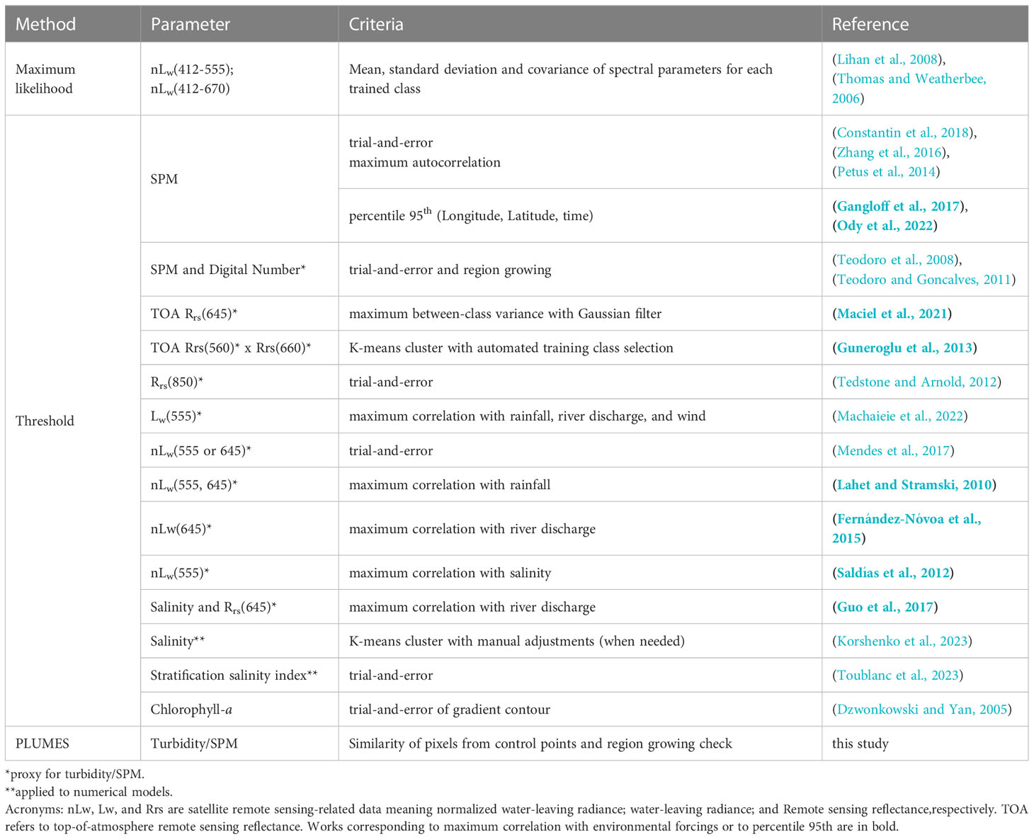
Table 1 Overview of the published studies on plume detection in coastal environments.

Of these known satellite remote sensing-based methods to delimit coastal plumes, all resort to a (necessary) degree of user supervision and most apply maximum likelihood technique or thresholds to establish the domain of plumes; approaches that have potential drawbacks due to their subjective nature. Maximum likelihood approach is usually carried out for multiple spectral products of the same time-step, in two phases: the training and the plume classification itself (either binary or with more classes). In a preliminary training phase, the statistical criteria for which the targeted features will be recognized are established. In the classification phase, these criteria are used according to where the probability of the likelihood of a pixel belonging to a pre-determined class is maximum. Guneroglu et al. (2013) further investigated the potential of automated class selection in the training phase. This automated process is followed by a K-means classification. Threshold techniques use a much simpler approach, by applying a pre-set value commonly determined from trial-and-error (e.g., Petus et al., 2014; Mendes et al., 2017; Toublanc et al., 2023) or statistical assumptions (e.g., Lahet and Stramski, 2010; Saldías et al., 2012; Gangloff et al., 2017; Maciel et al., 2021). It is, therefore, a challenging task to precisely extract coastal plumes for the same environment/site at different times using a pre-set value or trained class because turbidity is significantly different under different forcing mechanisms (e.g., seasonal variability, or changes due to extreme events). In that case, maximum likelihood approaches need to be re-trained (e.g., Thomas and Weatherbee, 2006) and thresholds must be adjusted not only for a specific site but case-by-case (e.g., Maciel et al., 2021), otherwise plumes may be overestimated, underestimated, or missed. To avoid overestimation, a few studies have further applied shallow water masks (typically< 20 m depth; e.g., Gangloff et al., 2017; Ody et al., 2022), manual adjustments (e.g., Korshenko et al., 2023), or region growing technique (e.g.,Teodoro et al., 2008; Teodoro and Goncalves, 2011); although the latter is less known for coastal applications but widely applied in the medical (e.g., Tariq et al., 2019; Kroon, 2022) and in spatial planning/cartography (e.g., Gonçalves, 2006). Application of shallow-water masks is intended to prevent the recurring issue that the thresholding method cannot distinguish between causes of turbid zones (i.e., turbid wakes, wave-driven coastal resuspension from the plume itself) like the human eye. For example, Gangloff et al. (2017) observed that shallow water masks lead to an underestimation by 20-100% in the Grand Rhône (France) for small plumes. Alternatively, the region growing technique, by assuming a spatially explicit context, may also assist in removing turbid zones that do not, in principle, belong to the region of plume influence. This region-growing technique scans for contiguous pixels according to a criterion of similarity (e.g., pixels below or above a threshold as in Teodoro et al., 2008; Teodoro and Goncalves, 2011) departing from a location of plume origin (also referred to as seed). In addition to the approaches mentioned, a new generation of artificial intelligence (AI) algorithms, including machine learning and deep learning, has been applied for the detection of various types of plumes such as volcanic ash (Guerrero Tello et al., 2022; Wilkes et al., 2022), fire smoke (Khan et al., 2021), atmospheric gases (Finch et al., 2022) or dust (Berndt et al., 2021) plumes. However, to the best of our knowledge, no studies have yet addressed the challenge of identifying turbid coastal plumes applying AI approaches.

This study presents a comparison of state-of-art threshold approaches and proposes a novel algorithm for coastal plume detection (PLUMES; PLUme Monitoring in Estuaries and Shelfs), discussing their advantages and limitations to identify plumes boundaries. The PLUMES algorithm proposes a semi-supervised statistically based and spatially explicit algorithm that does not assume a unique turbid plume characteristic. The Patos Lagoon turbid coastal plume, in southern Brazil, is used as a pilot application of the PLUMES algorithm and the applicability of the method to different estuaries and coastal shelfs is discussed.

2 Materials and Methods

2.1 Study site

This study focuses on the region of plume influence (ROPI) of the Patos Lagoon (Figure 1). Patos Lagoon is distinctively classified by Kjerfve (1986) as the largest choked coastal lagoon in the world, with about 250 km in length and 40 km in width. It is connected to the south Atlantic Ocean through a narrow inlet with less than 700 m width. This single inlet shelters the navigation channel of one of the most important commercial ports of southern Brazil, the Port of Rio Grande (Fernandes et al., 2021).

FIGURE 1

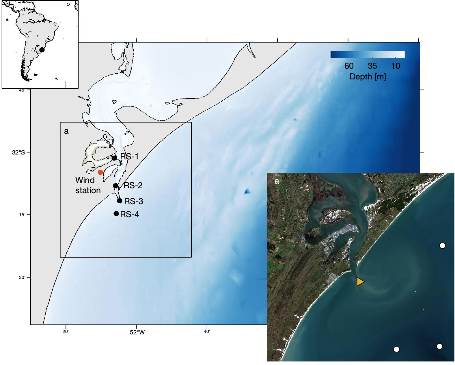
Figure 1 Estuary of Patos Lagoon, Brazil. Black circles represent the Buoy location (RS-1; RS-2, RS-3, and RS-4). Orange circle is the location of wind data station. In the Landsat-8 (Operational Land Imager – OLI) true-color composite of 2021-07-12, the dark-yellow triangle represents the control points used as plume origin and white-filled circles represent control point used as reference background marine waters inPLUMES algorithm (refer to Section 2.4.2). Landsat-8 image credit: USGS/NASA. Bathymetry data (depth) was provided by Brazilian Navy, Rio Grande Port Authority, Exclusive Economic Zone National Assessment Program (ReviZEE), and GEBCO and described by da Silva, et al. (2022) and da Silva et al. (2022).

The lagoon receives freshwater discharged from two main tributaries, Guaíba and Camaquã Rivers, and a smaller lagoon, Mirim Lagoon, through the São Gonçalo Channel. Freshwater flow to the Patos Lagoon varies with season. High values ~3000 m³s^-1 are discharged during the wet season (late winter and early spring), followed by low-to-moderate flow ~700 m³s^-1 during the dry season (summer and autumn) (Moller et al., 2001; Fernandes et al., 2021). Of the tributaries, Guaíba River is known for its largest contribution of suspended sediment inputs to the system. The region is affected by two meteorological systems, the South Atlantic anticyclones and those of polar origin, which dictates shifts in the prevailing NE winds (Moller et al., 2001) to S-SW on a time scale from days to weeks (Moller et al., 1996). The NE-SW wind regime is responsible for saltwater intrusion in the estuarine zone (Moller et al., 2001; Bitencourt et al., 2020) or freshwater extrusion (plume formation) and for vertical salinity gradients (Moller and Fernandes, 2010).

The Patos Lagoon exhibits a microtidal regime, with a mean range of 0.5 m and diurnal dominance (Moller et al., 2001), having negligible influence on the lagoon’s circulation (Moller et al., 2001; Fernandes et al., 2004). As the tidal amplitude is small, the dynamics of the lagoon and turbid plume is controlled by the combined effect of wind and river discharge: high river discharge (Q > 2,000 m³s^-1) overrules the dynamics promoted by winds, whereas, in dry periods, the wind effect becomes the most important forcing mechanism (Fernandes et al., 2002). Marques et al. (2010a) verified the importance of the river discharge intensity to its formation and Zavialov et al. (2018) identified the importance of the local wind action promoting the plume’s stratification (Zavialov et al., 2018). More recently, Bortolin et al. (2022) observed that seasonal and interannual forcings combined (related to El Niño Southern Oscillation), developed configurations of high and low discharge responsible for formation of turbid coastal plumes and their spread within Patos Lagoon and in the inner continental shelf. The authors also provided in their Supplementary Material a full time series of true-color composites from Landsat-5, -7, -8 between 1984 and 2020, providing overview of Patos Lagoon coastal ROPI.

2.2 In-situ data

In-situ data comprises time series of turbidity (T) as a surrogate parameter for SPM, river discharge, and winds. Turbidity data was available from the database SIstema de Monitoramento da COSTA Brasileira (SIMCOSTA¹) in the period 2016-2021 for four moored stations (see Figure 1 for locations): Station 1 (buoy RS-1) is located near the limit of the lower estuary, station 2 located in the navigation channel (buoy RS-2), station 3 located at the mouth of the estuary (buoy RS-3), and an offshore station 4 (buoy RS-4). Each in-situ station consists of meteo-oceanographic buoys conditioned to a sampling frequency of 30 minutes. The RS-1 station has a LOBO type buoy (Land/Ocean Biogeochemical Observatory), measuring turbidity with a resolution of 0.1 NTU at a wavelength of 700 nm and the RS-2 and RS-4 stations work with the Axys type buoy, using the Eco-Triplet optical sensor to measure turbidity at a wavelength of 700 nm. The SIMCOSTA dataset consists of latitude and longitude; collection date (second, minute, hour, day, month, and year), and a series of quality control tests (namely Gross Range Test; Spike Test; Rate of Change Test; and Flat Line Test), attributing the flag values for each of the tests: 1 (passed), 2 (not analyzed), 3 (suspect), 4 (failed) and 9 (missing data). Here we only keep data with flags attributed as 1.

Among the drivers of the estuarine dynamics, daily river discharge was recorded in the gauging stations in each of the lagoon’s tributaries (i.e., from 2013 to 2021) and made available from Agência Nacional de Águas (ANA²) for Guaíba and Camaquã rivers. River discharge from São Gonçalo Chanel was estimated through a rating curve method (Oliveira et al., 2015) applied to water level data available from Agência de Desenvolvimento da Lagoa Mirim (ALM). The sum of all three river discharges was applied. Hourly wind data from 2013-2021 were obtained from Instituto Nacional de Meteorologia (INMET³) from Rio Grande (station A802).

2.3 Remote sensing data and processing of turbidity estimates

Initially, all available level 1 satellite scenes from Landsat-8 (2013-2021), were obtained from the United States Geological Survey (USGS⁴). Landsat-8 being part of a long-term constellation of satellite sensors (since the 80’s), represents an important tool for coastal management. These images were atmospherically corrected using POLYMER, a software developed and maintained by HYGEOS⁵. POLYMER was chosen for the best fit with in-situ turbidity data in Patos Lagoon compared with results in (Tavora et al., 2023). Further, flags were checked for each scene and pixels were removed where atmospheric correction flags were indicating atmospheric artifacts.

Water reflectance from these satellite scenes were then compared with in-situ turbidity data at equivalent dates following good-practices recommended in IOCCG (2019): (1) the minimum time difference (i.e.,< 30 min), seeking to apply the comparison with the maximum of matching properties, (2) 3-by-3-pixel windows centered at the in-situ data location, (3) with a coefficient of variation lower than 0.25, and (4) at least 50% of valid pixels within a sampling box.

Using the match-up data, the semi-analytical algorithm described in Nechad et al. (2009) (Eq. 1) was empirically calibrated by applying a least squares minimization with a cost function (Eq. 2). The approach determines the best fitted coefficients (A and C) that represent in-situ turbidity data of Patos Lagoon.

$\begin{array}{ll}T= \frac{\left(A \times {\rho }_w\right)}{1- \frac{{\rho }_w}{C}}& \text{Eq. 1}\end{array}$

$\begin{array}{ll}{\chi }^2={\sum }_{i=1}^n\left[{\left(T_{i{n}_{situ}}(i)- T(i)\right)}^2\right]& \text{Eq. 2}\end{array}$

where A (NTU) and C (-) are regionally calibrated coefficients computed from the minimization and limited to positive values, ρ_w is median water reflectance (-), T_in-situ is in-situ turbidity (NTU) and n is number of match-ups available.

We split the number of matchups between validation and calibration sets: 70% of total matchups were used for calibration of A and C, while the remaining (30% of total match-up points) was used to test and confirm the accuracy achieved by the regionally calibrated coefficients. After, turbidity (NTU) maps were applied to every scene using newly estimated A and C coefficients (refer to Supplementary Material 1 for coefficients and match-up comparison). Lastly, the turbidity maps were inspected for missing spots from masked cloud disturbances within the coastal plume domain and removed. This is a necessary step because maps presenting such atmospheric artifacts may deteriorate the identification of the shape of the plume and lead to underestimation of its area (e.g., Petus et al., 2014). Remaining turbidity maps total 61.

2.4 Methods to detect turbid coastal plumes

2.4.1 Traditional state-of-art approaches for plume detection

Traditionally, thresholds are employed for the detection of turbid coastal plumes from satellite remote sensing (Ody et al., 2016; Gangloff et al., 2017; Maciel et al., 2021). Hereafter, we employ two of the most used approaches to detect the plumes and compare results with the proposed PLUMES method, MAXcorr, (Guo et al., 2017; Machaieie et al., 2022) and P95 (Gangloff et al., 2017). In MAXcorr, the threshold is obtained from the highest correlation with local driving mechanisms of river discharge and wind. The method assumes that the spatial magnitude and intensity of a given plume is a function of the forcing mechanisms acting upon the coastal environment. Here we applied the MAXcorr method by setting the range of turbidity thresholds to vary between 1 and 50 NTU, while allowing an average lag response for river discharge (1-30 days) and wind speed (1-24 hours) prior to satellite overpass. The obtained turbidity threshold presents the combination of forcings with the maximum correlations. The maximum correlation is determined by multiplying the correlations determined from each parameter. In the P95 method, the threshold is estimated from the 95th percentile of satellite-derived turbidity. The approach assumes that turbid coastal plumes are limited to highest turbidity values within the distribution by taking the 5% highest values (i.e., percentile 95th). The unique threshold is defined from the stack of satellite turbidity scenes in all three dimensions (i.e., latitude, longitude, time) to reach the 95th percentile. Gangloff et al. (2017) also observed that turbid coastal plumes contemplate two parts: a distal part (delimited by the P95 threshold) characterized as the largest coastal plume domain surrounded by less turbid plume boundaries due to suspended sediment settling and/or mixing with the ambient marine waters, and a proximal part (or the core) characterized by boundaries of higher turbidity and a smaller region contained within the distal plume domain. To identify the proximal part, authors have applied the 90th percentile of turbidity within each detected distal plume, resulting on a scene-by-scene proximal plume threshold.

2.4.2 The novel algorithm for plume detection: PLUMES

In this work we propose a spatially explicit time-resolved method to detect coastal plumes, the PLUMES algorithm (Figure 2). The PLUMES algorithm, in a similar fashion to supervised classification, starts by requesting a selection of control points from the stack of satellite turbidity maps: (i) in the origin of the turbid plume, such as a coastal inlet or river mouth and (ii) where turbid plumes do not occur, representing the background marine waters and the offshore coastal water. We recommend that the selection of such control points should be carried out by inspecting the stack of satellite-based scenes (for example the mean and standard deviation maps; refer to Figure SM2) to determine the ROPI and aid in the decision of control point’s location. We suggest observing preferable direction of plume deflection, zones of constant resuspension and navigation route of ships. The control point located at the origin of the plume should specially consider the direction of plume deflection (likely represented by highest mean turbidity and standard deviation). Concerning the selection of control points representing background marine waters (likely represented by lowest mean turbidity and standard deviation), we recommend the selection of two or more control points to capture most of the background marine spatial variability and prevent missing pixels from cloud cover. For the same reason, we also recommend that the marine control points are selected not as points grouped in a small location of the satellite scene, in the sense that the more spread these control points are, less likely they will capture the same cluster of missing pixels. For the application in the Patos Lagoon turbid plume, we selected one control point in the origin of the plume and three control points in the region of background marine waters (refer to Figure 1 for location of reference points used). Also note that the turbidity values of control points vary from image to image because turbidity is linked to the local hydrological and meteorological settings.

FIGURE 2

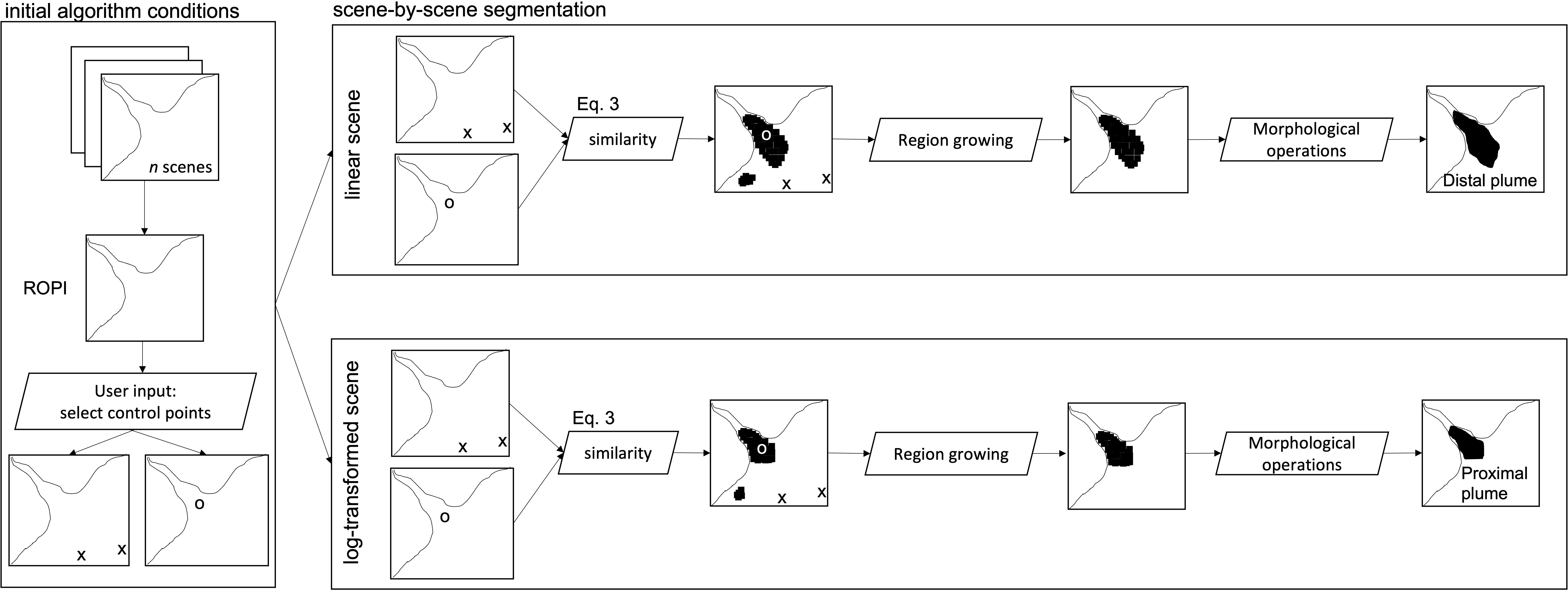
Figure 2 Flowchart of the algorithm framework split into two main parts (1) user-dependent initial algorithm conditions by defining the ROPI and location of control points from stack of n scenes, and (2) scene-by-scene image segmentation. ‘o’ shape represents pixel origin (or seed), and ‘x’ shape represents control points of region representing non-plume pixels. See also PLUMES algorithm available as a package of MATLAB functions (https://github.com/julianatavora/PLUMES_algorithm).

Once the location of control points is determined, these control points are checked if there are enough data points within a 5-by-5 window centered at each control point to be able to continue (we recommend the use of a n-by-n window to capture the noise of the sample in each control point, something not possible with the selection of a single pixel). For application in Patos Lagoon, the selection of control points resulted in 25 pixels located in the plume origin and 75 pixels representing background marine waters.

Within the limits of the (5-by-5 pixels) control points, if the number of missing values surpasses a pre-set threshold of 35%, the satellite scene is flagged, otherwise the statistical parameters (median, standard deviation and variance of the 5-by-5 pixels) within the turbid plume and non-plume samples are calculated. After checking for a minimum quantity of valid pixels within control points, a second criteria must be met: turbidity intensity must be higher in the control point set at the origin than the intensity set for the background marine waters. The assumption relies in the fact that a turbid coastal plume must be more turbid than its background marine waters.

For each turbidity map, the control points are grown to delineate the region belonging to the turbid plume and the region of non-plume by applying a measure of similarity of pixels in each scene (Eq. 3). This measure of similarity considers the squared difference between the pixel intensity and the median of the control point weighted by its measure of variability.

$\begin{array}{ll}{M}_{(i,j)}= \{\begin{array}{ll}plume, \hfill & \frac{{(I_{(i,j)}- {\mu }_{origin})}^2}{{\sigma }_{origin}}<\frac{{(I_{(i,j)}- {\mu }_{marine})}^2}{{\sigma }_{marine}}\hfill \\ non-plume,\hfill & otherwise\hfill \end{array}& \text{Eq. 3}\end{array}$

where M_{(i,j) is} the binary image (classes plume versus non-plume) indexed at pixel position (i,j) at each satellite scene (I), μ is the median of the control points (plume or non-plume), σ is the measure of variability of the control points.

This recently determined plume is referred to as the distal plume. Within the domain of the distal plume, the PLUMES algorithm also determines the proximal plume (also known as the core of the plume). While the former is determined using the linear-scale turbidity map, the proximal plume region is determined using log-transformed turbidity maps. The reason to use log-transformed turbidity is that relative to the median turbidity of the distribution, it increases the difference among low turbidity values and approximates higher turbidity values facilitating the detection of the region of highest turbidity (the proximal plume).

Further, within the PLUMES algorithm, the region growing algorithm, adapted from the original algorithm by Kroon (2022), runs a final check in the neighboring pixels of the already segmented turbid plume region (both distal and proximal plumes), which is set to grow from the control point known as the origin of the turbid plume; consolidating the plume feature. Finally, a table of plume metrics, some of which inspired on Gangloff et al. (2017) (i.e., area, orientation, plume centroid, mean, maximum, and minimum turbidity, and turbidity of control points) is returned to the user.

2.5 Sensitivity of plume detection to control points

Sensitivity analyses were conducted to determine how the detection of plumes by the PLUMES algorithm is affected by the choice of control points and window size (location in Figure 3), and thus provide a strategy for the choice of control points. The sensitivity analysis here consists of three groups of tests. The first group (Group 1) evaluated the impact of setting marine control points at varying distances from the control point at plume origin, aligned perpendicular to the coastline orientation, with a total of five tests. The second group (Group 2), consisting of three tests, uses a jackknife approach by removing one of the three marine control points while maintaining the control point at the plume origin. The third group (Group 3) performed two tests, the first consisting of a random selection of a new control point located at the plume’s origin while retaining the marine control points, followed by selecting three new control points located furthest offshore. Each sensitivity test was performed using different window sizes (3-by-3, 5-by-5, and 7-by-7 pixels), to evaluate sensitivity to window size. In total, 33 sensitivity runs were performed, with results presented in terms of the spatial distribution of plume occurrence (Supplementary Material 3) and the area of detected plumes.

FIGURE 3

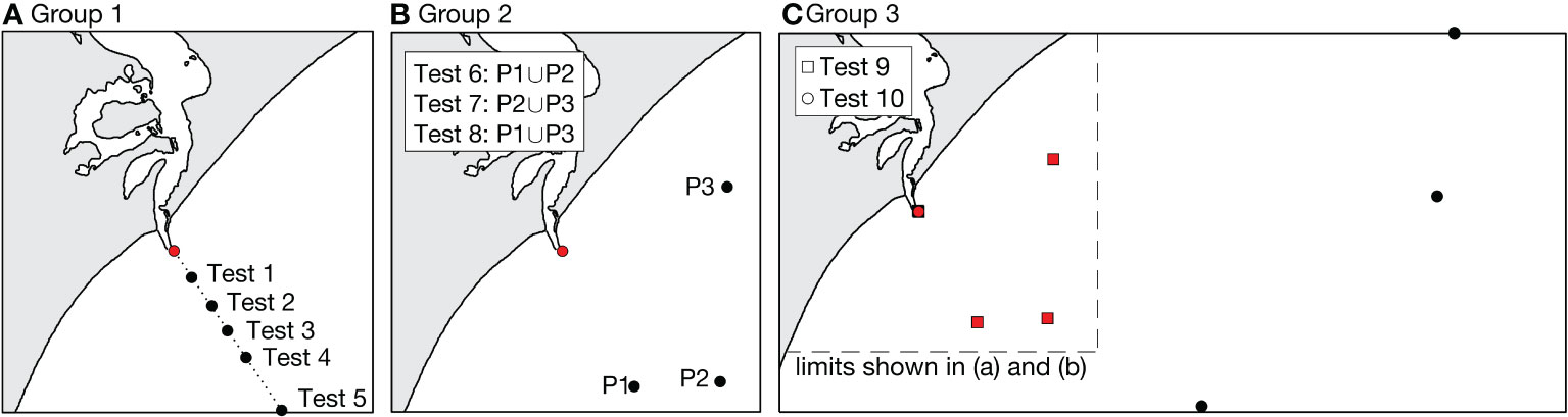
Figure 3 Location of control points by group of sensitivity tests: group 1 by changing distance (5, 10, 15, 20, and 30 km) of marine control points from the control point at plume origin (A), group 2 by removing one of the three marine control points selected (refer to Figure 1) at time (B), and group 3 (C) by selecting a new location for the control point at origin (Test 9 with square symbols) and selecting three new marine control points offshore (Test 10 with round symbols). Red symbols denote the same position of control points as in Figure 1, symbols in black denote locations have changed.

2.6 Performance assessment of detected plumes

2.6.1 Assessment of plume detection

How to determine to what extent a method for plume detection performs better than another? To date, there is no clear definition (and academic consensus) of what determines a plume’s limits from surface maps. In that sense, the process of validation of plume estimates is challenging (i.e., no ground-reference). However, we established a relative assessment by comparing the detection of turbid coastal plumes from both the PLUMES algorithm and thresholds (MAXcorr and P95) applied to the satellite-based turbidity maps. The congruence of detected plumes was assessed using the Intersection over Union (IoU) score. IoU score identifies the systematic difference among the detected features (Rezatofighi et al., 2019) and thereby is used to compare the detection of turbid plumes among approaches in this manuscript. The IoU score ranges from 0 (no overlap) to 1 (complete overlap of features). The high (low) scores however, in this study, do not imply correctness (wrongness) of one method over another but provide a clue to whether traditional and novel approaches detect similar structures or are similarly biased.

2.6.2 Criteria for assessment of limitations and advantages of approaches

Advantages and limitations of coastal plume detection were evaluated. First criteria for ease of assessment of coastal plumes were considered (i.e., lack of ground-reference, need for additional information). Second, the capacity of a method to extract spatial information, such as the ability to distinguish features and its computational costs. Thus, there are four key factors that were evaluated in this work, i.e., (1) Implementation: how easy is the approach to set up? (2) Effectiveness: does it need additional (subjective) input? Are there (site-specific) empirical assumptions? (3) Pitfalls/Strengths: do tools detect features not related to the plume (e.g., coastal resuspension), or can tools detect low turbidity plumes? (4) Speed: how fast is it to process a satellite image.

3 Results

3.1 Plumes detected from the traditional state-of-art thresholds

To determine appropriate threshold values for plume detection, statistical analysis was carried out examining the relationship between turbidity and two forcing mechanisms: river discharge and wind speed. Figure 4 shows the statistical results highlighting the correlations observed with river discharge (Figure 4A) and wind speed (Figure 4B). The analysis also revealed that the maximum correlation is found with river discharge (mean of river discharge 16 days previous to satellite overpass) and wind speed (mean of wind speed 6h previous to time of satellite overpass) with distal plume area (it should be noted that the MAXcorr approach does not detect proximal plumes).

FIGURE 4

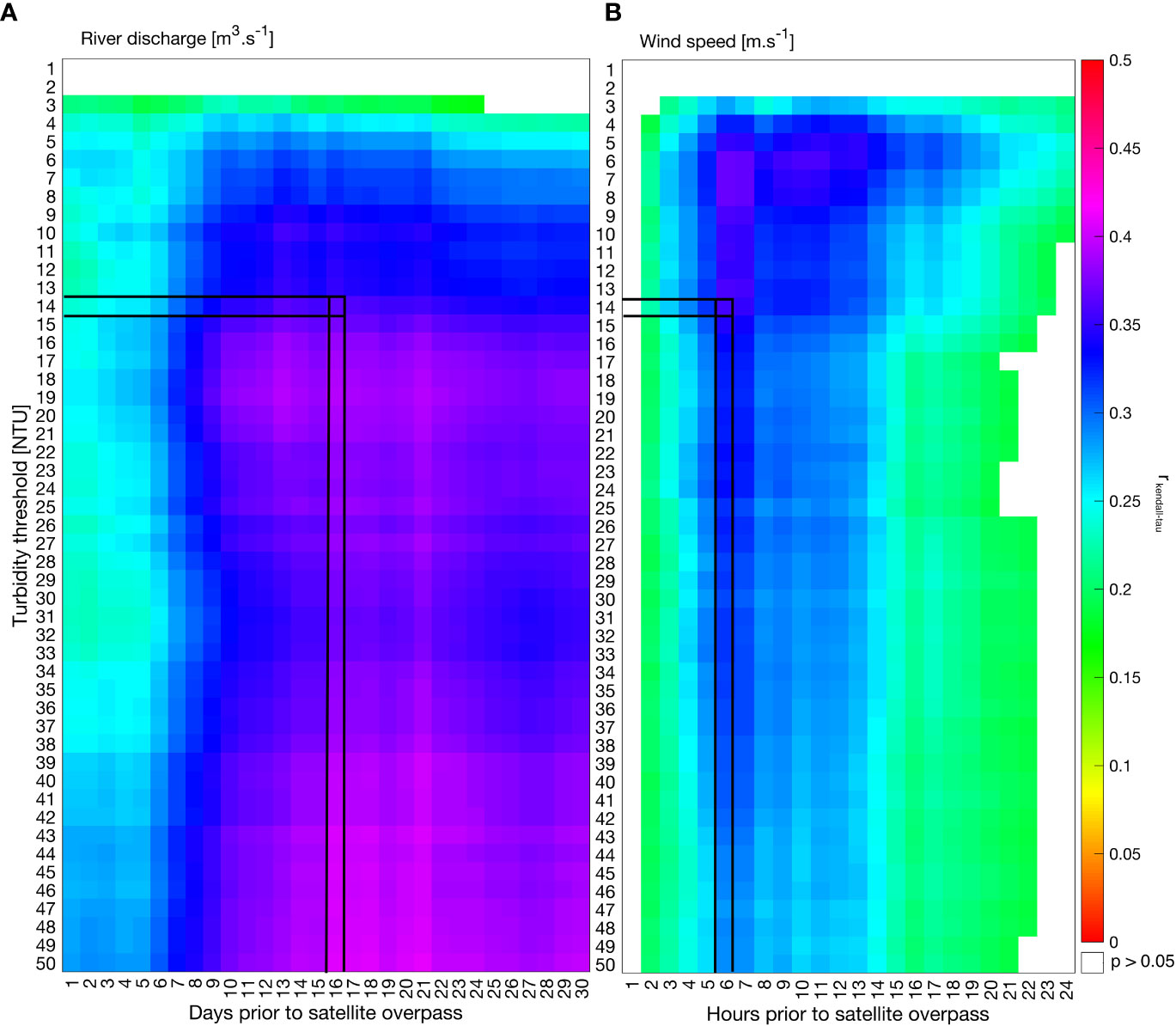
Figure 4 Heatmap of kendall-tau correlation coefficients (r) for the range of turbidity values (1-50 NTU) used as possible threshold to delimit Patos Lagoon coastal plume using inputs from (A) river discharge averaged over a range of 1 to 30 days prior to satellite overpass and (B) wind speed averaged over a range of 1 to 24 hours prior to satellite overpass. Values estimated as the maximum relationship (i.e., maximum values observed from the linear correlations estimated from river discharge versus turbidity and linear correlations estimated from wind speed versus turbidity) are marked by dark black lines, pointing convergence point. Regions in white represent r for which p-value < 0.05.

In addition to the statistical analysis applied in MAXcorr approach, an alternative approach was employed to explore the threshold of turbidity: P95. P95 was carried out considering the percentile 95^th of distribution of turbidity in both spatial (latitude and longitude) and temporal dimensions (stack of satellite scenes). Overall, the MAXcorr and P95 methods yielded relatively similar thresholds for turbidity (14 NTU and 17.7 NTU, respectively) in the context of distal plume detection. Overall, each threshold approach demonstrates a particular advantage: while MAXcorr, in theory, estimates the maximum relationship with forcing mechanisms, the P95 approach allows for estimates of proximal plumes.

3.2 Plumes detected from the PLUMES algorithm

Contrary to the fixed boundary assumptions (i.e., thresholds), the PLUMES algorithm yields variable turbidity in the coastal plume boundary as it is set for each scene, while considering the spatial context of plume origin. Figure 5 depicts the range of turbidities in the automatically retrieved plume metrics (Figure 5A; e.g., area, centroid, mean intensity), the range of turbidities of control points (Figure 5B) and the variability of turbidity in the determined boundaries (both distal and proximal plumes; Figure 5C). The results presented below are relative to a total of 59 scenes. Out of 61 satellite-based maps of turbidity, two scenes were flagged as they did not meet the pre-set criteria for plume detection of valid pixels (scene of May 24, 2018, with 40% of missing pixels) and intensity ratio (scene of March 29, 2021).

FIGURE 5

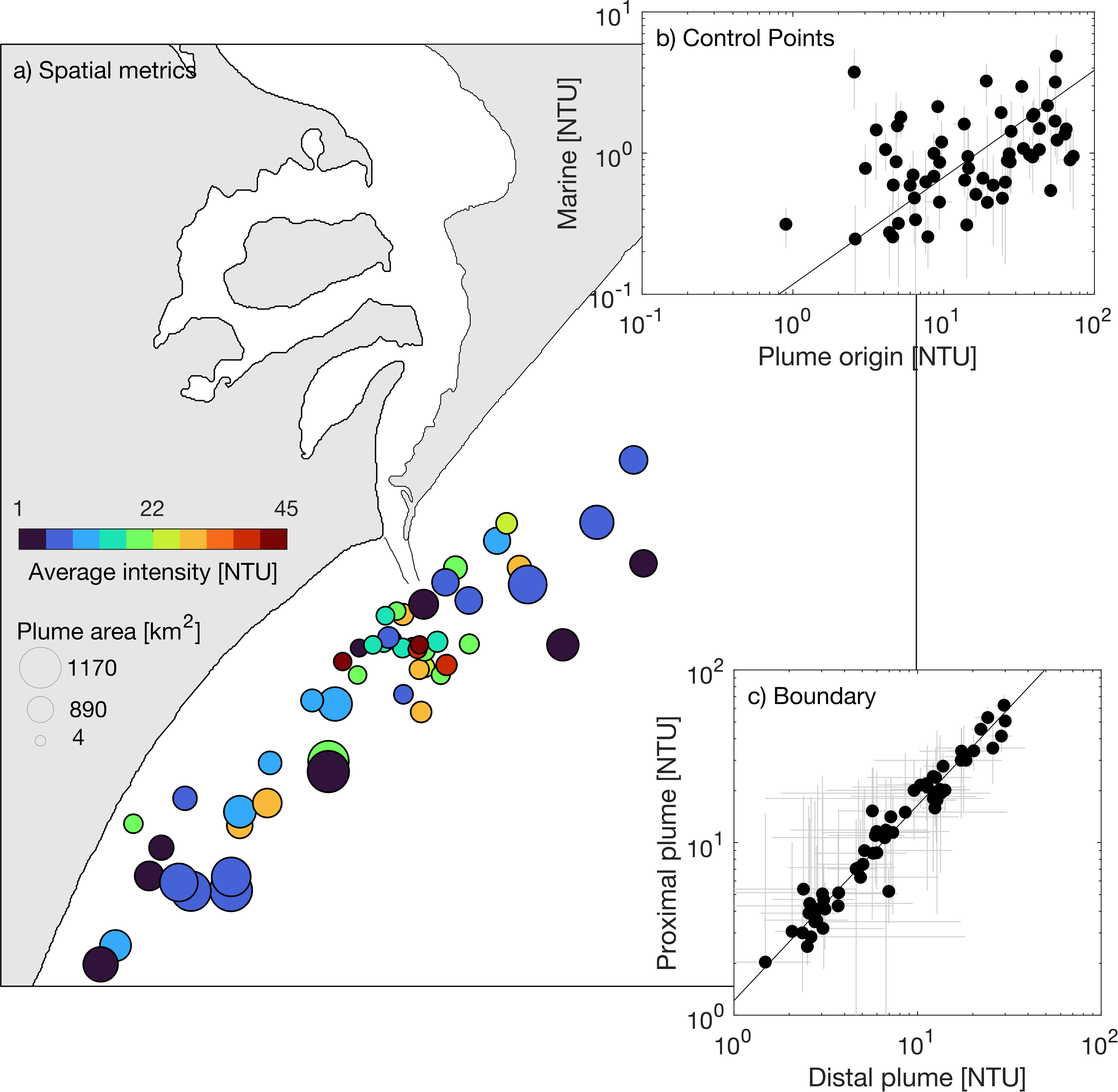
Figure 5 Metrics of turbid coastal plumes detected from the novel PLUMES algorithm summarized as spatial variability (A) of the plume’s centroids (location of scatted points) color-coded by average plume intensity and sizes representing the area of detected plumes. In-set panels depict median turbidity of control points (B; r kendall-tau = 0.31, p> 0.001) and mean turbidity of plumes boundaries (C; r kendall-tau = 0.85, p> 0.001). Vertical and horizontal bars in (B, C) represent standard deviation.

3.2.1 Sensitivity of PLUMES to the choice of control points

Tests to investigate the sensitivity of the PLUMES algorithm to the selection of control points revealed two main results: variable rate of flagged plumes (i.e., plumes unidentified) and the spatial variability of detected plumes (Figure 6; Figure SM3). Overall, test 1 (marine control point 5km from plume origin) and test 10 (marine control points selected furthest from origin) represent the most extreme selection of marine control points, yielding extreme results (both in area and number of detected plumes). Of these two tests, test 1 resulted in about 30% of flagged plumes and smallest plumes, while test 10 resulted in the largest plumes detected (two folds larger than the reference shown in Figure 6A). Thus, choosing marine control points too close to the plume origin will likely lead to misdetection of turbid plumes by either flagging their occurrence (especially failing the criteria of ratio of control points) or estimating smaller domains (Figure 6A), while choosing marine control points too far offshore will likely lead to estimating wider plume domains (Figure 6F). Remainder tests (2-9) did not yield significantly different results.

FIGURE 6

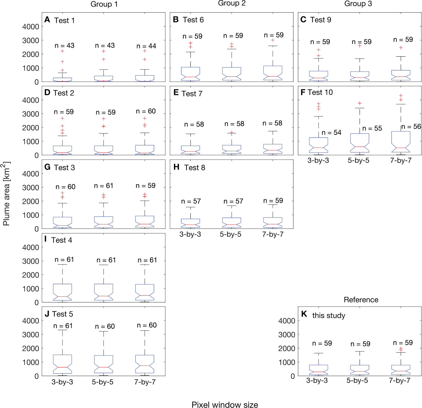
Figure 6 Comparison of area of detected plumes (in km2) from the sensitivity tests by changing control points location, number of control points, and window-size of control points (denoted by 3-by-3, 5-by-5 and 7-by-7). The selection of control points used in this sensitivity test is depicted in Group 1 (A, D, G, I, J) and Group 2 (B, E, H), Group 3 (C, F) and the reference (panel (K), adopting control points as in Figure 1). Refer to Figure 3 for location of control points in Group 1 and 2. Note that the number of plumes detected in each test is shown by each boxplot (denoted by n). An n below 61 (total number of satellite scenes) means that scenes had plume undetected (i.e., flagged) by failing the criteria established in the PLUMES algorithm.

Concerning pixel window size, overall, larger pixel window sizes yielded slightly larger plumes, while the number of flagged plumes was not largely affected.

3.3 Differences and similarities of detected plumes

Significant coastal turbidity events along-shore are registered by the three approaches (Figure 7) with comparable total area of plume occurrence (pixels where at least once a plume was detected). The PLUMES algorithm estimated the largest plume boundaries both for proximal and distal plumes. Yet, the percentage of occurrence of plumes is at least twice as low when applying MAXcorr and P95 than the PLUMES algorithm (Figure 7C versus Figures 7A, B), particularly in the region near the inlet (the plume origin). This is observed for both distal and proximal plumes. Additionally, the percentage of occurrence of proximal plumes applying PLUMES (Figure 7E) seems more comparable with distal plumes identified by applying the threshold approaches (Figures 7A, B). This similarity between proximal plume from PLUMES (Figure 7C) with distal plumes from MAXcorr and P95 (Figures 7A, B) may be an indication that the latter two approaches are biased towards detecting turbidity-rich coastal plumes while missing low turbidity plumes.

FIGURE 7

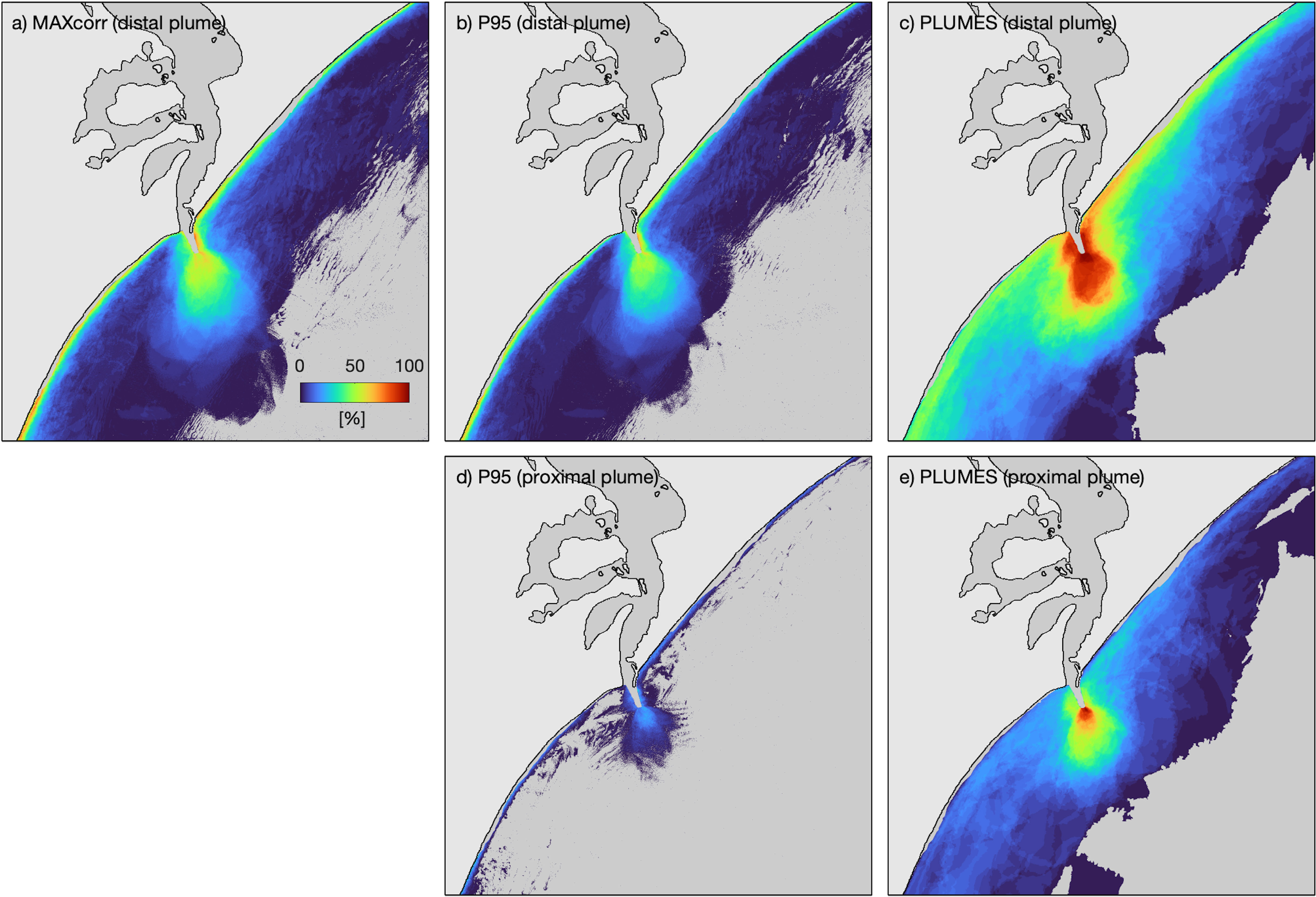
Figure 7 Overall congruence of plumes (maps of percentage of plume occurrence by approach). Top panels (A–C) depict the detected distal plumes and bottom (D, E) depict proximal plumes. Panels (A) depicts plumes detected from the MAXcorr approach, (B, D) depict plumes detected from the P95 approach, and (C, E) plumes detected from the PLUMES approach. MAXcorr has not a methodology for proximal plume estimates.

To further investigate the comparability of plumes from different methods, and their overlap, we compared the area of identified distal plumes using the IoU scores (Figures 8A–C) and turbidity at the control point of plume origin (Figures 8D–F). Generally, good agreement of detected areas is reported with a high IoU score (IoU > 0.8). This good agreement is observed between MAXcorr and P95 over the entire range of plume’s areas, implying that these approaches provide similar results. PLUMES, on the other hand, yielded larger plume areas for many scenes. Figures 8D, E shows the pattern of low turbidity (mostly below 18 NTU) in the plume origin for scattered points that do not fall within good agreement of detected plume area (seemingly overestimation of plumes, see also Figure 9) whereas no pattern is observed from median turbidity of marine control points in Supplementary Material 4.

FIGURE 8

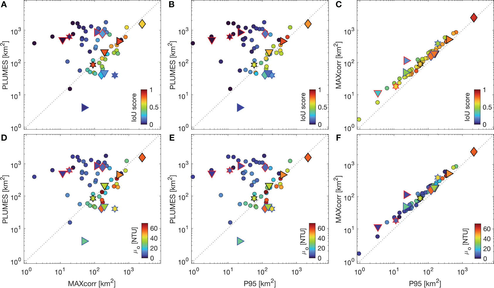
Figure 8 Area of detected distal plumes from each of the approaches, color-coded with IoU (Intersection over Union) scores (A–C) and color-coded with median turbidity (in NTU) of PLUMES’s control point at origin (m_o; D–F). Symbols contoured in red represent snapshots in Figure 9; in blue (Figure 10) and in black (Figure 11). Different symbols represent different dates of plumes in each figure.

FIGURE 9

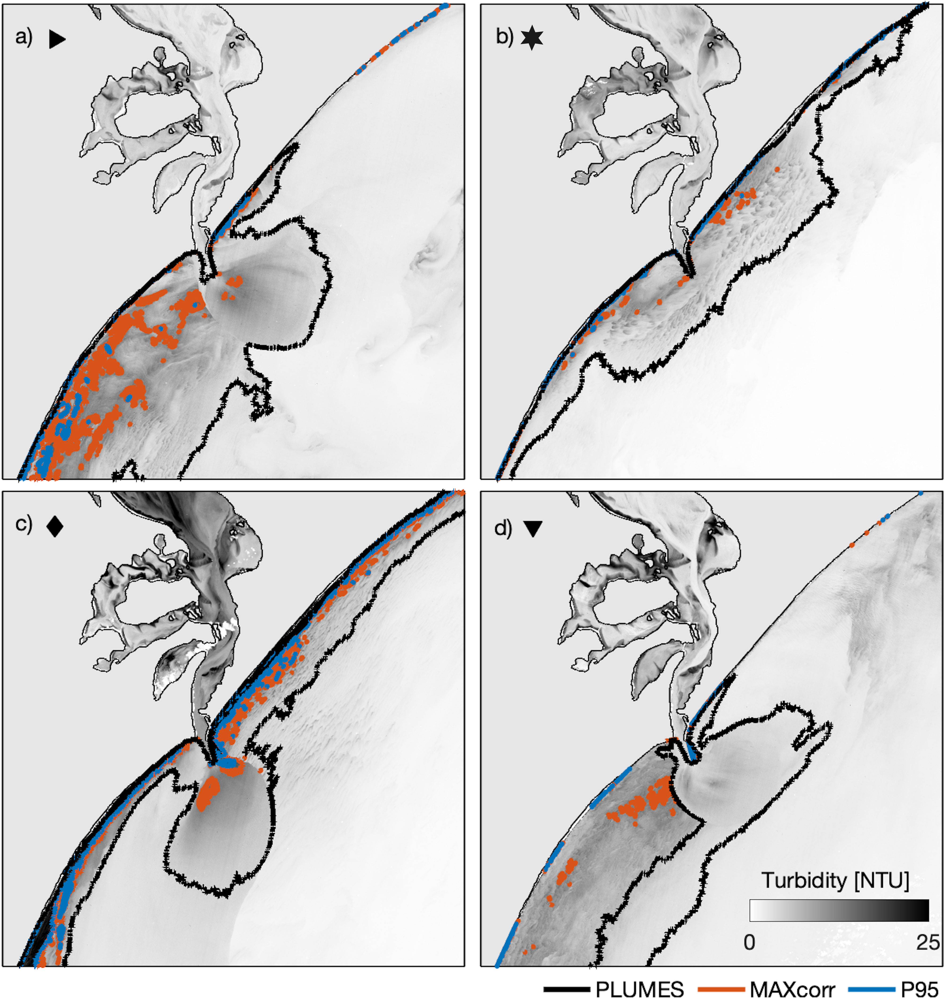
Figure 9 Examples of scenes which detected plume seem overestimated (IoU score< 0.2) from PLUMES algorithm compared with P95 and MAXcorr based on IoU score. (A–D) respectively depict scenes of 2015-06-01, 2016-02-28, 2021-05-16 and 2018-02-17. The IoU score of each scene is highlighted in Figure 8 with the respective red-contour symbols. Black line represents the boundaries of plumes detected with PLUMES algorithm, dark orange represents boundaries of plumes from MAXcorr threshold, and blue boundaries are plumes from P95 threshold.

As observed in Figure 8, for several scenes, the PLUMES algorithm detects larger (Figure 9) or smaller (Figure 10) distal plumes compared to either MAXcorr or P95, while in other cases, results of the three approaches are similar (Figure 11). We inspected examples of each of these three groups in detail. Figure 9 depicts four examples of low turbidity scenes for which case plumes are underestimated by MAXcorr and P95 approaches relative to PLUMES. These are majorly represented by a low IoU score (< 0.2, i.e., little limited overlap of detected plume areas between methods) and plumes with boundaries of turbidity below the defined thresholds (explaining the low retrieval of plume features by MAXcorr and P95). Contrastingly, Figure 10 depicts four examples of apparent relative overestimation by PLUMES (0.2 > IoU > 0.8, moderate to good overlap of plumes), where MAXcorr and P95 consistently detect fragments of coastal resuspension or clusters of pixels above threshold (e.g., Figure 10C). These examples demonstrate how PLUMES may aid in preventing the detection of non-plume coastal features. Figure 11 depicts examples of good agreement between PLUMES with MAXcorr and P95 (IoU > 0.8, i.e., remarkably high overlap of detected plumes between methods). These are represented by moderate-to-high turbidity and relatively sharper boundaries compared to the previous examples.

FIGURE 10

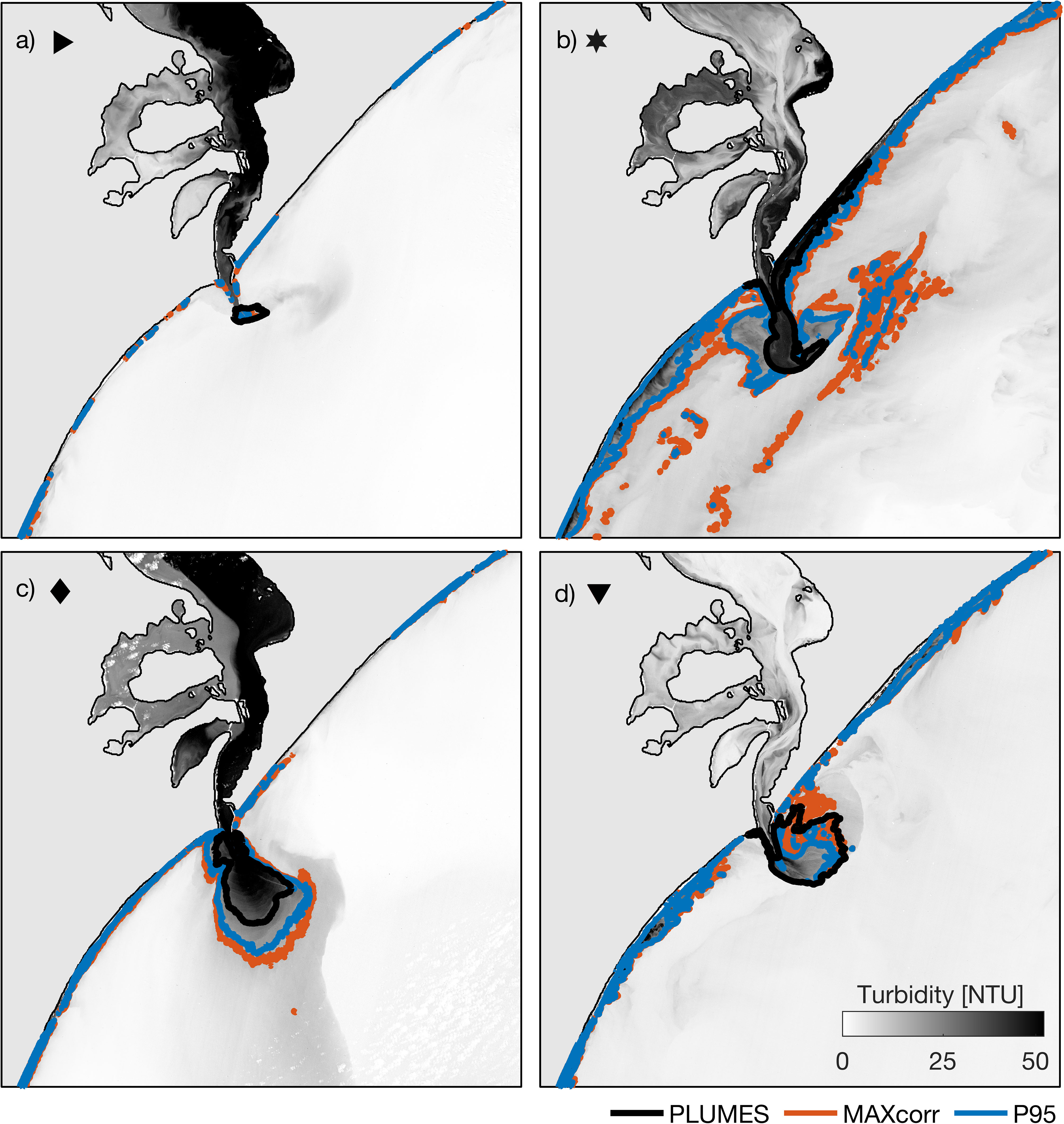
Figure 10 Examples of scenarios which detected plumes are underestimated (0.2 > IoU > 0.8) from PLUMES algorithm compared with MAXcorr and P95. (A–D) respectively depict scenes of. 2015-12-10, 2016-08-22, 2019-11-19, and 2020-05-29. The IoU score of each scene is highlighted in Figure 8 with the respective blue-contour symbols. Black line represents the boundaries of plumes detected with PLUMEs algorithm, dark orange represents boundaries of plumes from MAXcorr threshold, and blue boundaries are plumes from P95 threshold. Attention for the coastal resuspension detected with MAXcorr and P95.

FIGURE 11

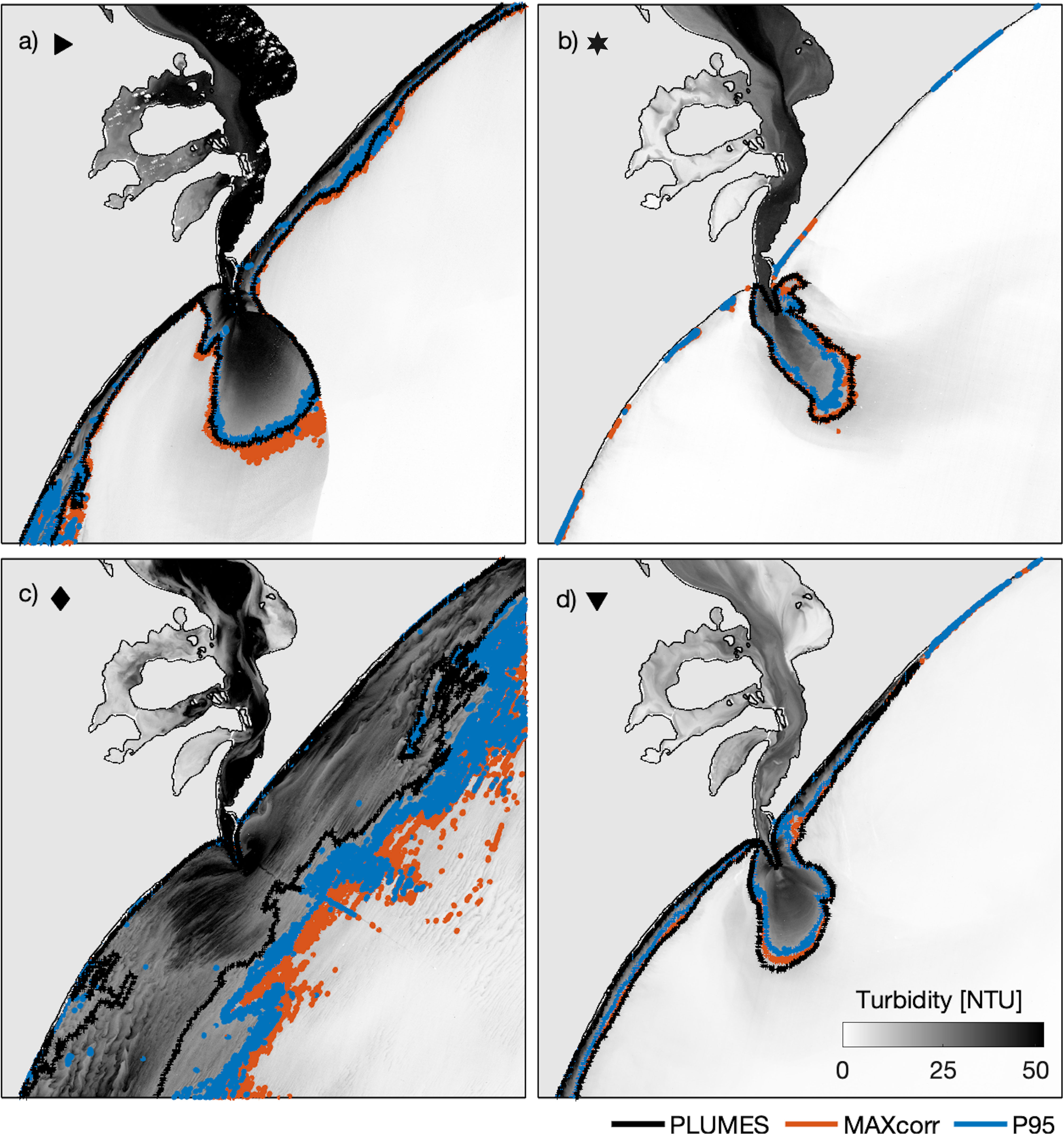
Figure 11 Examples of scenes which detected plume yielded an IoU score > 0.8, i.e., good correspondence among the three algorithms. (A–D) respectively depict scenes of 2013-11-18, 2016-06-19, 2020-06-14, 911 and 2020-09-18. The IoU score of each scene is highlighted in Figure 8 with the respective black-contour symbols. Black line represents the boundaries of plumes detected with PLUMEs algorithm, dark orange represents boundaries of plumes from MAXcorr threshold, and blue boundaries are plumes from P95 threshold. Attention for the coastal resuspension detected with MAXcorr and P95.

4 Discussion

4.1 Challenges and outlook of detecting turbid coastal plumes

Defining turbid coastal plumes is not a trivial task Gangloff et al. (2017). Plume boundaries have been traditionally addressed relying on site-specific knowledge to define where a plume boundary most likely is (Constantin et al., 2018), but according to (Gangloff et al., 2017), different approaches for plume detection yield different results which may also differ from a plume manually drawn by an expert.

Nonetheless, what should/could be used to define a plume’s limits? Currently, in the absence of a definition of plume boundaries, one is left with the threshold-based approaches. Although these approaches are relatively simple to implement and have fast processing times, they are subjective. The threshold is likely to change based on the dataset available and timeframe analyzed. In this respect, the threshold needs to be identified for each new satellite acquisition that is added to the stack. As we have shown in this work (e.g., Figure 8) these approaches are prone to ignore less intense plumes or smaller highly turbid coastal plumes. This drawback has been addressed by other authors with the aid of additional site-specific adjustments to achieve higher accuracy and precision; e.g., shallow-water masks (Gangloff et al., 2017); noise-removal and region growing (Teodoro et al., 2008); manual adjustment of plume boundary (Korshenko et al., 2023).

It must be acknowledged that there will be scenarios where plume detection is challenged regardless of the employed plume detection method. For example, visually, plumes with sharp fronts are relatively easier to distinguish from the background marine waters compared to dissipating plumes where borders are fuzzy [Tariq et al. (2019) discusses the challenges of feature detection with sharp versus dissipating boundaries] and plume intensity is closer to the intensity of the background marine water (e.g., Figure 8D). We anticipate that certain scenarios may particularly increase the challenge, such as strong meteorological and hydrodynamic conditions (i.e., passage of polar systems; meteorological tides) that increase surface turbidity through wave-driven resuspension and/or prevent settling of particles while intensifying mixing and leading to dissipating plumes.

In the last couple of years, AI algorithms have been increasingly used for a wide range of applications. AI approaches have, to our knowledge, not been applied to detect the outline and spatial context of coastal plumes. This may be due to the more complex challenges posed by the dynamic nature of the water constituents in coastal areas and the atmosphere above it, as observed from satellite scenes. In this context, PLUMES, by considering the spatially explicit context of a turbid coastal plume, advances detection of turbid coastal plumes. Looking forward, PLUMES can benefit from potential automated control point selection, and/or future AI-based algorithms can benefit from the spatial explicitness provided by PLUMES in terms of training and cross-validation. However, such direction needs further investigation.

4.2 Advantages and potential limitations of PLUMES algorithm relative to MAXcorr and P95

In the PLUMES algorithm, we included several improvements over previous methods. Firstly, it is context-based and considers the neighboring pixels in each turbidity map, guaranteeing that the detected plume feature is spatially coherent. The approach reduces the likelihood of underestimating coastal plumes and capturing coastal resuspension. Secondly, PLUMES determines two plume features: distal and proximal plume and provides an overview of detected metrics. Thirdly, it has a plurality of satellite sensors and water quality applications based on intensity, including sea surface temperature and colored organic matter plumes.

Previously published methods for plume detection perform best under a relatively narrow suite of conditions (i.e., site and dataset dependent). Indeed, for the Gironde Estuary, three studies have reported varied thresholds for plume detection (e.g., Constantin et al. (2018) applied a threshold of 8 g.m^-3, Castaing et al. (1999) a threshold of 3 FTU, while Lafon (2009) indicated a range between 6 and 10 g.m^-3) all of which were applied to different datasets. Furthermore, Teodoro and Goncalves (2011) reported the threshold approach was found to be invalid for comparing different years of the same dataset in the Douro River. These examples demonstrate the non-trivial task of assuming a uniform threshold value for turbid plume detection, highlighting the advantages of using algorithms like PLUMES that can accommodate varying conditions. Aiming on providing more accurate and comparable results, PLUMES was set-up to be used as a time-step-based algorithm allowing to consider the spatial variability of turbidity conditions at each time-step (scene) independently.

While PLUMES has been applied to Landsat in this study, PLUMES also has, as have the state-of-the-art threshold methods, potential for use with other sensor data. Applying the PLUMES algorithm, we compared results from Landsat-8 scenes as described in this study, to Sentinel-2 scenes in the same day overpass. Refer to Supplementary Material 5 for processing of Sentinel-2 turbidity and to Figures SM6-A and SM6-B for comparison between Landsat-8 and Sentinel-2 detected plumes. We observed that one plume with complex features was not detected (failing the region growing step) and the remaining comparative scenes yielded overall good agreement among distal plumes. Results in Figures SM6-A, B suggest a potential multiplicity of satellite sensors available to PLUMES.

However, the effectiveness of PLUMES detecting turbid coastal plumes is dependent on the selection of control points that accurately represent the classes to be segmented (i.e., plume versus non-plume). The optimal number of control points, their location in a satellite scene or turbidity map of coastal plume, and the appropriate window size for each control point are important considerations for successful plume detection (for which we recommend the use of composite maps of mean and standard deviation from the stack of scenes). While at least one control point within the turbid coastal plume domain and one control point representing the non-plume region are necessary, selecting more control points can capture more of the coastal variability and prevent flagging. For instance, in this study three control points were used for Patos Lagoon in the background marine waters, leading to better plume detection. Although theoretically a single-pixel control point can be effective in detecting plumes, it is not recommended due to noise in satellite image acquisition (Tariq et al., 2019). Thus, it is recommended to use larger window sizes, such as 5-by-5 or 7-by-7, when segmenting noisy images (Adams and Bischof, 1994).

To establish control points that accurately represent turbid coastal plumes and their variability, we suggest performing a few training tests by modifying the location, number, or window size of control points. This process of testing and modifying control points, similar to a sensitivity test, allows the optimization of the PLUMES algorithm’s performance specific to the site being studied. This level of human input grants the PLUMES algorithm a semi-supervised characteristic. It is important to note that a certain level of user input is always required for image segmentation (Adams and Bischof, 1994) and the difference between the trial-and-error criteria of setting thresholds and selecting control points for region growing algorithms is that the effect of control points selection allows for targeted classification of images being particularly useful for complex or irregular features (Adams and Bischof, 1994) such as turbid coastal plumes. Once a set of control points is established, PLUMES can discriminate non-plumes from turbid plumes for all scenes. Note that literature offers a few options for automated selection of control points (e.g., Fan et al., 2005; Gómez et al., 2007) but these methods primarily focus on application for objects with sharp boundaries. As a result, they are not yet suited for application in turbid coastal plumes.

While it is important to acknowledge the limitations of any algorithm or approach, it is also important to recognize its strengths and potential applications. The PLUMES algorithm, for instance, can be a powerful tool for detecting turbid coastal plumes in satellite images, which can have significant implications for coastal management. The PLUMES also takes advantage of the region growing approach (mostly popular in the medical field and urban planning) by removing fragments that, in principle, do not belong within the coastal plume domain, provided that they are not attached to the plume. However, PLUMES has not yet been tested for plume detection in other study sites and requires a certain level of user input. Thresholds, on the other hand, are widely applied and are simple to implement (particularly P95, as no further assumptions and calculations need to be made) offering fast processing times (which can be useful when operating large datasets). Briefly we provide a table summarizing criteria and scores of each plume detection approach (Table 2).

TABLE 2

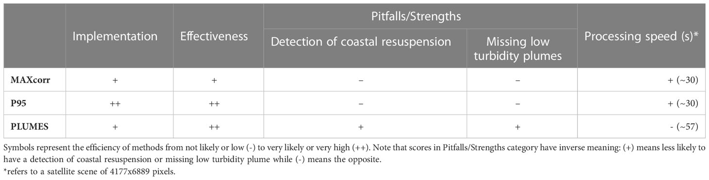
Table 2 Pertinence of each tested plume detection approach regarding the four selected criteria.

Finally, the PLUMES methodology, similarly to P95 or MAXcorr, offers an adaptable approach for implementation in regions experiencing plumes and requires a collection of satellite scenes that captures temporal changes within the plume domain. The difference is that PLUMES, beyond analyses of the stack of satellite scenes to depict the spatial and temporal variability within the ROPI, requires the selection of control points in the plume origin and in background marine waters. This selection depends on the river or estuary configuration (e.g., narrow inlet, funnel-shaped), and preferable direction of plume deflection, furthest extension of turbid plumes, or bathymetry favoring coastal resuspension (e.g., location of nearshore bars and shoals). To aid on the spatial understanding of turbid plumes, composite maps of mean and standard deviation are recommended. For Patos Lagoon, plume origin was observed as region of both highest mean turbidity and standard deviation whereas marine control points, representing background waters, were observed as regions of lowest mean turbidity and standard deviation. The inclusion of sensitivity tests is also important during this step to assess the detection of plume boundaries. While the PLUMES algorithm has potential to be transferable to other regions with plumes, further research is needed to test its robustness.

5 Synthesis and conclusions

Diverse methodologies have been employed in coastal regions to understand the dynamics of turbid coastal plumes from satellite remote sensing with thresholds being the most frequent approach. Here we provide a novel satellite-based algorithm called PLUMES, designed for monitoring of turbid coastal plumes such as the Patos Lagoon coastal plume. The PLUMES algorithm relies on a semi-supervised approach for selection of control points that will be used as references to detect a turbid coastal plume. The selection of these control points is a crucial step in achieving improved results. The PLUMES exhibits several advantages, including lower likelihood of missing low turbidity plumes (such as the ones with turbidity boundaries below threshold) and detecting coastal resuspension or other coastal features detached from the turbid coastal plume. Notably, the versatility of PLUMES is not limited to Landsat-8, however the longer time-series will likely provide a better spatial and temporal understanding of plume configuration.

The scope of application of PLUMES potentially extends beyond the identification of feature detection (and their metrics) in turbidity maps and is likely not limited to satellite-based products alone. PLUMES may be applied to analyze various parameters such as algal blooms, sea surface temperature, salinity fields, and even oil spills, as extracted from satellite remote sensing maps or numerical models. Therefore, the approach suggested here can serve as a simple, yet (potentially) versatile tool for coastal management. To enhance the detection of coastal features further, future research could involve integrating artificial intelligence (AI) techniques and further testing the robustness of the method for monitoring turbid coastal plumes in other study sites.

6 Software availability

PLUMES software will be available as a package of MATLAB functions under https://github.com/julianatavora/PLUMES_algorithm. Project partners are welcome to contribute to this open-source package (e.g., by implementing their site-specific plume detection as an add-on; converting PLUMES to Python or Google Earth Engine languages; or recommending additional features). Practical examples of the PLUMES application will be available within the subfolder “Examples”.

Data availability statement

The raw data supporting the conclusions of this article will be made available by the authors, without undue reservation.

Author contributions

JT: Conceptualization, methodology, writing—original draft, writing—review and editing, validation, formal analysis. GG: Conceptualization, methodology. EF: Conceptualization, methodology, writing—review and editing. MS: Conceptualization, methodology, writing—review and editing, supervision. DW: Conceptualization, methodology, writing—review and editing, supervision. All authors have read and agreed to the published version of the manuscript. All authors contributed to the article and approved the submitted version.

Acknowledgments

The authors are grateful to USGS/NASA for openly providing Landsat-8 imagery, to PEPS and European Space Agency/Copernicus for providing Sentinel-2 imagery; to SIMCOSTA, ANA and INMET for the in-situ data; to HYGEOS for POLYMER atmospheric correction; to the LOAD Project - Long-term analysis of Suspended Particulate Matter Concentrations Affecting port areas in Developing countries (ONR grant N62909-19-1-2145). EF is a CNPq research fellow (PQ2 No 304684/2022-8). The authors would like to thank the reviewers for the insightful contributions.

Conflict of interest

The authors declare that the research was conducted in the absence of any commercial or financial relationships that could be construed as a potential conflict of interest.

Publisher’s note

All claims expressed in this article are solely those of the authors and do not necessarily represent those of their affiliated organizations, or those of the publisher, the editors and the reviewers. Any product that may be evaluated in this article, or claim that may be made by its manufacturer, is not guaranteed or endorsed by the publisher.

Supplementary material

The Supplementary Material for this article can be found online at: https://www.frontiersin.org/articles/10.3389/fmars.2023.1215327/full#supplementary-material

Footnotes

1. ^ https://simcosta.furg.br/home (accessed on 3 February, 2022).
2. ^ https://www.gov.br/ana/pt-br (accessed on 26 January, 2023).
3. ^ https://mapas.inmet.gov.br (accessed on 26 January, 2023).
4. ^ https://earthexplorer.usgs.gov/ (accessed on 3 November, 2022).
5. ^ https://www.hygeos.com/polymer.

References

Adams R., Bischof L. (1994). Seeded region growing. IEEE Trans. Pattern Anal. Mach. Intell. 16, 641–647. doi: 10.1109/34.295913

CrossRef Full Text | Google Scholar

Berndt E. B., Elmer N. J., Junod R. A., Fuell K. K., Harkema S. S., Burke A. R., et al. (2021). A machine learning approach to objective identification of dust in satellite imagery. Earth Sp. Sci. 8, e2021EA001788. doi: 10.1029/2021EA001788

CrossRef Full Text | Google Scholar

Bitencourt L. P., Fernandes E. H. L., Dias da Silva P., Moller O. O. (2020). Spatio-temporal variability of suspended sediment concentrations in a shallow and turbid lagoon. J. Mar. Syst. 212, 103454. doi: 10.1016/j.jmarsys.2020.103454

CrossRef Full Text | Google Scholar

Bortolin E. C., Tavora J., Fernandes E. H. L. (2022). Long-term variability on suspended particulate matter loads from the tributaries of the world’s largest choked lagoon. Front. Mar. Sci. 9. doi: 10.3389/fmars.2022.836739

PubMed Abstract | CrossRef Full Text | Google Scholar

Castaing P., Froidefond J. M., Lazure P., Weber O., Prud’Homme R., Jouanneau J. M. (1999). Relationship between hydrology and seasonal distribution of suspended sediments on the continental shelf of the Bay of Biscay. Deep. Res. Part II Top. Stud. Oceanogr. 46, 1979–2001. doi: 10.1016/S0967-0645(99)00052-1

CrossRef Full Text | Google Scholar

Ciotti Á. M., Odebrecht C., Fillmann G., Moller O. O. (1995). Freshwater outflow and subtropical convergence influence on phytoplankton biomass on the southern Brazilian continental shelf. Cont. Shelf Res. 15, 1737–1756. doi: 10.1016/0278-4343(94)00091-Z

CrossRef Full Text | Google Scholar

Constantin S., Doxaran D., Derkacheva A., Novoa S., Lavigne H. (2018). Multi-temporal dynamics of suspended particulate matter in a macro-tidal river plume (the gironde) as observed by satellite data. Estuar. Coast. Shelf Sci. 202, 172–184. doi: 10.1016/j.ecss.2018.01.004

CrossRef Full Text | Google Scholar

da Silva D. V., Oleinik P. H., Costi J., de Paula Kirinus E., Marques W. C., Moller O. O. (2022). Variability of the spreading of the Patos Lagoon plume using numerical drifters. Coasts 2, 51–69. doi: 10.3390/coasts2020004

CrossRef Full Text | Google Scholar

da Silva P. D., Fernandes E. H., Gonçalves G. A. (2022). Sustainable development of coastal areas: Port expansion with small Impacts on estuarine hydrodynamics and sediment transport pattern. Water 14, 3300. doi: 10.3390/w14203300

CrossRef Full Text | Google Scholar

Dzwonkowski B., Yan X.-H. (2005). Tracking of a Chesapeake Bay estuarine outflow plume with satellite-based ocean color data. Cont. Shelf Res. 25, 1942–1958. doi: 10.1016/j.csr.2005.06.011

CrossRef Full Text | Google Scholar

Fan J., Zeng G., Body M., Hacid M. S. (2005). Seeded region growing: an extensive and comparative study. Pattern Recognit. Lett. 26, 1139–1156. doi: 10.1016/j.patrec.2004.10.010

CrossRef Full Text | Google Scholar

Fernandes E. H. L., da Silva P. D., Gonçalves G., Möller O. (2021). Dispersion plumes in open ocean disposal sites of dredged sediment. Water 13, 808. doi: 10.3390/w13060808

CrossRef Full Text | Google Scholar

Fernandes E. H. L., Dyer K. R., Moller O. O., Niencheski L. F. H. (2002). The Patos Lagoon hydrodynamics during an El Niño event, (1998). Cont. Shelf Res. 22, 1699–1713. doi: 10.1016/S0278-4343(02)00033-X

CrossRef Full Text | Google Scholar

Fernandes E. H. L., Mariño-Tapia I., Dyer K. R., Moller O. (2004). The attenuation of tidal and subtidal oscillations in the Patos Lagoon estuar. Ocean Dyn. 54, 349–359. doi: 10.1007/s10236-004-0090-y

CrossRef Full Text | Google Scholar

Fernández-Nóvoa D., Mendes R., deCastro M., Dias J. M. M., Sánchez-Arcilla A., Gómez-Gesteira M. (2015). Analysis of the influence of river discharge and wind on the ebro turbid plume using MODIS-aqua and MODIS-Terra data. J. Mar. Syst. 142, 40–46. doi: 10.1016/j.jmarsys.2014.09.009

CrossRef Full Text | Google Scholar

Finch D. P., Palmer P. I., Zhang T. (2022). Automated detection of atmospheric NO2 plumes from satellite data: a tool to help infer anthropogenic combustion emissions. Atmos. Meas. Tech. 15, 721–733. doi: 10.5194/amt-15-721-2022

CrossRef Full Text | Google Scholar

Gangloff A., Verney R., Doxaran D., Ody A., Estournel C. (2017). Investigating rhône river plume (Gulf of Lions, France) dynamics using metrics analysis from the MERIS 300m Ocean Color archive, (2002–2012). Cont. Shelf Res. 144, 98–111. doi: 10.1016/j.csr.2017.06.024

CrossRef Full Text | Google Scholar

Gómez O., González J. A., Morales E. F. (2007). “Image segmentation using automatic seeded region growing and instance-based learning,” in Progress in pattern recognition, image analysis and applications (Berlin, Heidelberg: Springer Berlin Heidelberg), 192–201. doi: 10.1007/978-3-540-76725-1_21

CrossRef Full Text | Google Scholar

Gonçalves G. A. (2006). Detecção automática de alterações na cartografia cadastral com base em imagens de câmeras digitais. PhD thesis. Universidade Federal do Paraná. Available at: http://hdl.handle.net/1884/10825.

Google Scholar

Guerrero Tello J. F., Coltelli M., Marsella M., Celauro A., Palenzuela Baena J. A. (2022). Convolutional neural network algorithms for semantic segmentation of volcanic ash plumes using visible camera imagery. Remote Sens. 14, 4477. doi: 10.3390/rs14184477

CrossRef Full Text | Google Scholar

Guneroglu A., Karsli F., Dihkan M. (2013). Automatic detection of coastal plumes using Landsat TM/ETM+ images. International J. Remote Sens 34 (13), 4702-4714. doi: 10.1080/01431161.2013.782116

CrossRef Full Text | Google Scholar

Guo K., Zou T., Jiang D., Tang C., Zhang H. (2017). Variability of Yellow River turbid plume detected with satellite remote sensing during water-sediment regulation. Cont. Shelf Res. 135, 74–85. doi: 10.1016/j.csr.2017.01.017

CrossRef Full Text | Google Scholar

Horner-Devine A. R., Hetland R. D., MacDonald D. G. (2015). Mixing and transport in coastal river plumes. Annu. Rev. Fluid Mech. 47, 569–594. doi: 10.1146/annurev-fluid-010313-141408

CrossRef Full Text | Google Scholar

IOCCG (2019). Uncertainties in ocean colour remote sensing. report ser. Ed. Mélin F. (Dartmouth, Canada: International Ocean Color Coordinating Group). doi: 10.25607/OBP696

CrossRef Full Text | Google Scholar

Khan S., Muhammad K., Hussain T., Ser J., Cuzzolin F., Bhattacharyya S., et al. (2021). DeepSmoke: deep learning model for smoke detection and segmentation in outdoor environments. Expert Syst. Appl. 182, 115125. doi: 10.1016/j.eswa.2021.115125

CrossRef Full Text | Google Scholar

Kjerfve B. (1986). Comparative oceanography of coastal lagoons. In Wolfe D. A. ed. Estuarine Variability, New York: Academic Press, 63–81. doi: 10.1016/B978-0-12-761890-6.50009-5

CrossRef Full Text | Google Scholar

Klemas V. (2012). Remote sensing of coastal plumes and ocean fronts: overview and case study. J. Coast. Res. 28, 1–7. doi: 10.2112/JCOASTRES-D-11-00025.1

CrossRef Full Text | Google Scholar

Korshenko E., Panasenkova I., Osadchiev A., Belyakova P., Fomin V. (2023). Synoptic and seasonal variability of small river plumes in the northeastern part of the Black Sea. Water 15, 721. doi: 10.3390/w15040721

CrossRef Full Text | Google Scholar

Kroon D.-J. (2022) Region growing. Available at: https://www.mathworks.com/matlabcentral/fileexchange/19084-region-growing.

Google Scholar

Lafon V. (2009) Expoitation des données MODIS pour la zone gironde - marennes-oléron. G.E.O. transfert. UMR 5805 EPOC, Université Bordeaux, document interne, p.40. Available at: https://www.scopus.com/inward/record.uri?eid=2-s2.0-85044343989&partnerID=40&md5=81ae56cfe2a62cd166b6024d222e67b2.

Google Scholar

Lahet F., Stramski D. (2010). MODIS imagery of turbid plumes in San Diego coastal waters during rainstorm events. Remote Sens. Environ. 114, 332–344. doi: 10.1016/j.rse.2009.09.017

CrossRef Full Text | Google Scholar

Lee J., Valle-Levinson A. (2013). Bathymetric effects on estuarine plume dynamics. J. Geophys. Res. Ocean. 118, 1969–1981. doi: 10.1002/jgrc.20119

CrossRef Full Text | Google Scholar

Lihan T., Saitoh S. I., Iida T., Hirawake T., Iida K. (2008). Satellite-measured temporal and spatial variability of the Tokachi River plume. Estuar. Coast. Shelf Sci. 78, 237–249. doi: 10.1016/j.ecss.2007.12.001

CrossRef Full Text | Google Scholar

Machaieie H. A., Nehama F. P. J., Silva C. G., de Oliveira E. N. (2022). Satellite assessment of coastal plume variability and its relation to environmental variables in the Sofala Bank. Front. Mar. Sci. 9. doi: 10.3389/fmars.2022.897429

PubMed Abstract | CrossRef Full Text | Google Scholar

Maciel F. P., Santoro P. E., Pedocchi F. (2021). Spatio-temporal dynamics of the río de la plata turbidity front; combining remote sensing with in-situ measurements and numerical modeling. Cont. Shelf Res. 213, 104301. doi: 10.1016/j.csr.2020.104301

CrossRef Full Text | Google Scholar

Marques W. C., Fernandes E. H. L., Moller O. O. (2010a). Straining and advection contributions to the mixing process of the Patos Lagoon coastal plume, Brazil. J. Geophys. Res. 115, C06019. doi: 10.1029/2009JC005653

CrossRef Full Text | Google Scholar

Marques W. C., Fernandes E. H. L., Monteiro I. O., Möller O. O. (2009). Numerical modeling of the Patos Lagoon coastal plume, Brazil. Cont. Shelf Res. 29, 556–571. doi: 10.1016/j.csr.2008.09.022

CrossRef Full Text | Google Scholar

Marques W. C., Fernandes E. H. L., Moraes B. C., Moller O. O., Malcherek A., Möller O. O., et al. (2010b). Dynamics of the Patos Lagoon coastal plume and its contribution to the deposition pattern of the southern Brazilian inner shelf. J. Geophys. Res. Ocean. 115, 1–22. doi: 10.1029/2010JC006190

CrossRef Full Text | Google Scholar

Mendes R., Saldías G. S., deCastro M., Gómez-Gesteira M., Vaz N., Dias J. M. (2017). Seasonal and interannual variability of the douro turbid river plume, northwestern Iberian Peninsula. Remote Sens. Environ. 194, 401–411. doi: 10.1016/j.rse.2017.04.001

CrossRef Full Text | Google Scholar

Moller O. O., Castaing P. (1999). “Hydrographical characteristics of the estuarine area of Patos Lagoon (30{\textdegree}S, Brazil),” in Estuaries of south America: their geomorphology and dynamics. Eds. Perillo G. M. E., Piccolo M. C., Pino-Quivira M. (Berlin, Heidelberg: Springer Berlin Heidelberg), 83–100. doi: 10.1007/978-3-642-60131-6_5

CrossRef Full Text | Google Scholar

Moller O. O., Castaing P., Salomon J.-C., Lazure P. (2001). The influence of local and non-local forcing effects on the subtidal circulation of Patos Lagoon. Estuaries 24, 297. doi: 10.2307/1352953

CrossRef Full Text | Google Scholar

Moller O. O., Fernandes E. H. L. (2010). “Pesquisa Ecológica de Longa Duração - PELD,” in O Estuário da lagoa dos patos: um século de transformaçōes. Eds. Seelinger U., Odebrecht C. (Rio Grande: FURG), 17–40.

Google Scholar

Moller O. O., Lorenzzentti J. A., Stech J., Mata M. M. (1996). The Patos Lagoon summertime circulation and dynamics. Cont. Shelf Res. 16, 335–351. doi: 10.1016/0278-4343(95)00014-R

CrossRef Full Text | Google Scholar

Monteiro I. O., Marques W. C., Fernandes E. H. L., Gonçalves R. C., Moller O. O., Möller O. O. (2011). On the effect of earth rotation, river discharge, tidal oscillations, and wind in the dynamics of the Patos Lagoon coastal plume. J. Coast. Res. 27, 120–130. doi: 10.2112/JCOASTRES-D-09-00168.1

CrossRef Full Text | Google Scholar

National Oceanic Atmospheric Administration, (NOAA) (2006). Fisheries glossary. river plume. NOAA technical memorandum NMFS-F/SPO-69. Revised edition. Available at: https://repository.library.noaa.gov/view/noaa/12856.

Google Scholar

Nechad B., Ruddick K. G., Neukermans G. (2009). Calibration and validation of a generic multisensor algorithm for mapping of turbidity in coastal waters. Remote Sens. Ocean. Sea Ice Large Water Reg. 2009, 7473, 74730H. doi: 10.1117/12.830700

CrossRef Full Text | Google Scholar

Ody A., Doxaran D., Vanhellemont Q., Nechad B., Novoa S., Many G., et al. (2016). Potential of high spatial and temporal ocean color satellite data to study the dynamics of suspended particles in a micro-tidal river plume. Remote Sens. 8, 245. doi: 10.3390/rs8030245

CrossRef Full Text | Google Scholar

Ody A., Doxaran D., Verney R., Bourrin F., Morin G. P., Pairaud I., et al. (2022). Ocean color remote sensing of suspended sediments along a continuum from rivers to river plumes: concentration, transport, fluxes and dynamics. Remote Sens. 14, 2026. doi: 10.3390/rs14092026

CrossRef Full Text | Google Scholar

Oliveira H. A., De, Fernandes E. H. L., Möller O. O. Jr., Collares G. L. (2015). Processos hidrológicos e hidrodinâmicos da lagoa mirim. Revista Brasileira de Recursos Hídricos 20, 34–45. Available at: http://repositorio.furg.br/handle/1/5615.

Google Scholar

Osadchiev A., Sedakov R. (2019). Spreading dynamics of small river plumes off the northeastern coast of the Black Sea observed by Landsat 8 and Sentinel-2. Remote Sens. Environ. 221, 522–533. doi: 10.1016/j.rse.2018.11.043

CrossRef Full Text | Google Scholar

Osadchiev A., Zavialov P. (2020). “Structure and dynamics of plumes generated by small rivers,” in Estuaries and coastal zones - dynamics and response to environmental changes Eds. Pan J., Devlin A. (IntechOpen). doi: 10.5772/intechopen.87843

CrossRef Full Text | Google Scholar

Petus C., Marieu V., Novoa S., Chust G., Bruneau N., Froidefond J.-M. (2014). Monitoring spatio-temporal variability of the adour river turbid plume (Bay of Biscay, France) with MODIS 250-m imagery. Cont. Shelf Res. 74, 35–49. doi: 10.1016/j.csr.2013.11.011

CrossRef Full Text | Google Scholar

Rezatofighi H., Tsoi N., Gwak J., Sadeghian A., Reid I., Savarese S. (2019). Generalized intersection over union: a metric and a loss for bounding box regression. Proc. IEEE Comput. Soc Conf. Comput. Vis. Pattern Recognit. 2019-June, 658–666. doi: 10.1109/CVPR.2019.00075

CrossRef Full Text | Google Scholar

Saldías G. S., Sobarzo M., Largier J., Moffat C., Letelier R. (2012). Seasonal variability of turbid river plumes off central Chile based on high-resolution MODIS imagery. Remote Sens. Environ. 123, 220–233. doi: 10.1016/j.rse.2012.03.010

CrossRef Full Text | Google Scholar

Tariq H., Jilani T., Amjad U., Aqil Burney S. M. (2019). Novel seed selection and conceptual region growing framework for medical image segmentation. Brain Broad Res. Artif. Intell. Neurosci. 10, 6–19.

Google Scholar

Tavora J., Jiang B., Kiffney T., Bourdin G., Gray P. C., Carvalho L. S., et al. (2023). Recipes for the derivation of water quality parameters using the high-Spatial-Resolution data from sensors on board Sentinel-2A, Sentinel-2B, Landsat-5, Landsat-7, Landsat-8, and Landsat-9 satellites. J. Remote Sens. 3, 1–18. doi: 10.34133/remotesensing.0049

CrossRef Full Text | Google Scholar

Tedstone A. J., Arnold N. S. (2012). Automated remote sensing of sediment plumes for identification of runoff from the Greenland ice sheet. J. Glaciol. 58, 699–712. doi: 10.3189/2012JoG11J204

CrossRef Full Text | Google Scholar

Teodoro A., Goncalves H. (2011). “Extraction of Estuarine/Coastal environmental bodies from satellite data through image segmentation techniques,” in Image segmentation, ed. Ho P.-G. (InTech). doi: 10.5772/14672

CrossRef Full Text | Google Scholar

Teodoro A., Gonçalves H., Veloso-Gomes F., Gonçalves J. A. (2008). “Estimation of the douro river plume dimension based on image segmentation of MERIS scenes,” in Remote sensing for agriculture, ecosystems, and hydrology X. Eds. Neale C. M. U., Owe M., D’Urso G., 71040F. doi: 10.1117/12.799879

CrossRef Full Text | Google Scholar

Thomas A. C., Weatherbee R. A. (2006). Satellite-measured temporal variability of the Columbia River plume. Remote Sens. Environ. 100, 167–178. doi: 10.1016/j.rse.2005.10.018

CrossRef Full Text | Google Scholar

Toublanc F., Ayoub N. K., Marsaleix P. (2023). On the role of wind and tides in shaping the gironde river plume (Bay of Biscay). Cont. Shelf Res. 253, 104891. doi: 10.1016/j.csr.2022.104891

CrossRef Full Text | Google Scholar

Wilkes T. C., Pering T. D., McGonigle A. J. S. (2022). Semantic segmentation of explosive volcanic plumes through deep learning. Comput. Geosci. 168, 105216. doi: 10.1016/j.cageo.2022.105216

CrossRef Full Text | Google Scholar

Yuan J., Miller R. L., Powell R. T., Dagg M. J. (2004). Storm-induced injection of the Mississippi River plume into the open Gulf of Mexico. Geophys. Res. Lett. 31, 2–5. doi: 10.1029/2003GL019335

CrossRef Full Text | Google Scholar

Zavialov P. O., Kostianoy A. G., Möller O. O. (2003). SAFARI cruise: mapping river discharge effects on Southern Brazilian shelf. Geophys. Res. Lett. 30, 1–4. doi: 10.1029/2003GL018265

CrossRef Full Text | Google Scholar

Zavialov P. O., Pelevin V. V., Belyaev N. A., Izhitskiy A. S., Konovalov B. V., Krementskiy V. V., et al. (2018). High resolution LiDAR measurements reveal fine internal structure and variability of sediment-carrying coastal plume. Estuar. Coast. Shelf Sci. 205, 40–45. doi: 10.1016/j.ecss.2018.01.008

CrossRef Full Text | Google Scholar

Zhang Y., Shi K., Zhou Y., Liu X., Qin B. (2016). Monitoring the river plume induced by heavy rainfall events in large, shallow, Lake Taihu using MODIS 250m imagery. Remote Sens. Environ. 173, 109–121. doi: 10.1016/j.rse.2015.11.020

CrossRef Full Text | Google Scholar