Using age compositions derived from spatio-temporal models and acoustic data collected by uncrewed surface vessels to estimate Pacific hake (Merluccius productus) biomass-at-age

Generating biomass-at-age indices for fisheries stock assessments with acoustic data collected by uncrewed surface vessels (USVs) has been hampered by the need to resolve acoustic backscatter with contemporaneous biological (e.g., age) composition data. To address this limitation, Pacific hake (Merluccius productus; “hake”) acoustic data were gathered from a USV survey (in 2019) and acoustic-trawl survey (ATS; 2019 and eight previous years), and biological data were gathered from fishery-dependent and non-target (i.e., not specifically targeting hake) fishery-independent sources (2019 and eight previous years). To overcome the lack of contemporaneous biological sampling in the USV survey, age class compositions were estimated from a generalized linear mixed spatio-temporal model (STM) fit to the fishery-dependent and non-target fishery-independent data. The validity of the STM age composition estimation procedure was assessed by comparing estimates to age compositions from the ATS in each year. Hake biomass-at-age was estimated from all combinations of acoustics (USV or ATS in 2019, ATS only in other years) and age composition information (STM or ATS in all years). Across the survey area, proportional age class compositions derived from the best STM differed from ATS observations by 0.09 on average in 2019 (median relative error (MRE): 19.45%) and 0.14 across all years (MRE: 79.03%). In data-rich areas (i.e., areas with regular fishery operations), proportional age class compositions from the STM differed from ATS observations by 0.03 on average in 2019 (MRE: 11.46%) and 0.09 across years (MRE: 54.96%). On average, total biomass estimates derived using STM age compositions differed from ATS age composition-based estimates by approximately 7% across the study period (~ 3% in 2019) given the same source of acoustic data. When biomass estimates from different sources of acoustic data (USV or ATS) were compared given the same source of age composition data, differences were nearly ten-fold greater (22% or 27%, depending on if ATS or STM age compositions were used). STMs fit to non-contemporaneous data may provide suitable information for assigning population structure to acoustic backscatter in data-rich areas, but advancements in acoustic data processing (e.g., automated echo classification) may be needed to generate viable USV-based estimates of biomass-at-age.

1 Introduction

Autonomous vessels have shown great promise for enhancing ocean observation programs. Uncrewed surface vessels (USVs) are particularly useful for missions of long duration in harsh environments (Liu et al., 2016; Mordy et al., 2017; Meinig et al., 2019), and are well suited to carry out survey operations in circumstances that would limit or prevent the operation of crewed surveys (e.g., De Robertis et al., 2021). Therefore, USVs have been used to understand physical oceanography (Wills et al., 2021; Nickford et al., 2022; Zhang et al., 2022), animal distribution and behavior (De Robertis et al., 2019b; Verfuss et al., 2019; Levine et al., 2021), and collect data in service of fishery resource survey programs (Chu et al., 2019; De Robertis et al., 2021; Sepp et al., 2022). Incorporating USVs into fishery-independent survey programs is of particular interest given their potential to increase the efficiency of ship-based survey effort and mitigate the effects of unexpected circumstances (e.g., funding shortfalls, vessel unavailability).

Fishery-independent survey programs that generate indices for stock assessment typically rely on two types of data: (1) abundance or biomass and (2) composition (e.g., age, length, species composition). One gear can provide both types of data in some situations (e.g., trawls, stereo-video), but many survey programs employ multiple gears to collect sufficient data of each type. One of the most common combinations of gears is an acoustic-trawl survey (Simmonds and MacLennan, 2005), where trawls provide the much more broadly sampled acoustic backscatter with point samples of composition data that are extrapolated to estimate the biomass-at-age of target species. USVs can collect acoustic data in support of fishery resource survey programs but are ill-equipped to collect composition data, which has thus far limited their operational use. The study of De Robertis et al. (2021), which used an empirically derived relationship between acoustic backscatter and biomass to estimate the total biomass of Walleye Pollock (Gadus chalcogrammus) in Alaska, was a significant advancement towards providing data for stock assessments with USV surveys. However, as most modern stock assessments are age- or length-structured, providing a biomass index with a USV survey that is equivalent to one generated with a survey vessel requires biomass estimates to be resolved by age or length.

Spatio-temporal models (STMs) are statistical models that make highly resolved predictions based on spatial, temporal, and spatio-temporal effects. Accordingly, they may be suitable for estimating composition data for acoustic surveys when contemporaneous biological sampling is not possible. One type of STM, the vector autoregressive spatio-temporal (VAST) model, is particularly well-suited for integrating data from multiple sources, multi-variate applications, and generating robust indices in a variety of situations (Grüss and Thorson, 2019; Thorson, 2019; Brodie et al., 2020). Therefore, VAST models are commonly used to generate indices of biomass or abundance distribution (Thorson and Barnett, 2017; Godefroid et al., 2019; Thorson et al., 2021) and estimate diet and age-length-sex composition (Thorson and Haltuch, 2019; Grüss et al., 2020; O’Leary et al., 2020). If estimates of composition data derived from STMs such as VAST can be applied to acoustic data collected by USVs, the utility of USVs would be greatly expanded. Adding USV data collection could facilitate a higher level of spatial and temporal resolution in fishery resource surveys than adding additional crewed data collection given the same operational constraints (e.g., funding, person hours). The additional high-resolution data would support the next generation of spatially-resolved stock assessment and management strategies (Berger et al., 2017).

We aimed to determine if a combination of acoustic data from USVs and age compositions derived from a STM could generate viable estimates of Pacific hake (Merluccius productus; “hake”) biomass-at-age. Hake are the most abundant groundfish in the California Current Large Marine Ecosystem and support one of the largest fisheries on the U.S. West Coast south of Alaska (Hamel et al., 2015; NOAA, 2015; Johnson et al., 2021). Hake undertake a seasonal northward migration in the spring, where the extent of the migration is determined in part by age, size, and oceanographic conditions (Dorn, 1995; Hamel et al., 2015; Malick et al., 2020). The Joint U.S.-Canada Integrated Ecosystem and Pacific Hake Acoustic Trawl Survey (ATS) is conducted biennially in the summer months to estimate the biomass-at-age of the entire stock, which is managed and surveyed jointly by the U.S. and Canada. In 2019, a USV (Saildrone) acoustic survey was conducted in conjunction with the hake survey (de Blois, 2020).

The specific objectives of the present study were the following: (1) estimate hake age class composition with STMs fit to a combination of fishery-dependent and non-target fishery-independent age data, (2) estimate hake biomass-at-age from all combinations of acoustic (USV or ATS) and age composition information (STM or ATS), (3) compare the age compositions estimated in objective 1 with those of the ATS to evaluate the validity of age compositions estimated with STMs, and (4) compare total biomass estimates derived in objective 2 to determine the relative effects of differing sources of age composition and acoustic data on total biomass estimates. We completed these objectives with data from 2019, when the USV and ATS sampled the survey area in tandem, and for eight previous survey years (ATS vessel acoustics only) to examine if the performance of generating age compositions using STMs was reasonable and stationary under different conditions. If USV surveys are to be useful for age-resolved indices of abundance for stock assessment, there needs to be an understanding of the benefits, limitations, and efficiencies available to best leverage this technology and inform management decisions.

2 Methods

2.1 Study domain

This study took place in waters off the U.S. West Coast from 34.4 to 55.5° latitude and -135.5 to -120.6° longitude (Figure 1). Some datasets employed in this study covered this entire area, while others covered smaller portions of the survey domain. (Figure 1; described in greater detail below). For spatio-temporal modelling, we modified the spatial grid used to generate kriged biomass estimates from data collected in the ATS by Northwest Fisheries Science Center (National Marine Fisheries Service – National Oceanic and Atmospheric Administration; NWFSC) personnel (Chu et al., 2017). This grid was clipped to match the latitudinal extents of the U.S. West Coast and reached the 1500 m isobath or 35 nmi offshore, whichever was furthest offshore (Chu et al., 2017; de Blois, 2020). Grid cells were generally 21.4 km² except in areas where they conformed to the coastline or shelf contour. In some analyses, we made comparisons between predictions in geographic strata defined by the International Pacific Fisheries Council (INPFC), which are shown in Figure 1.

FIGURE 1

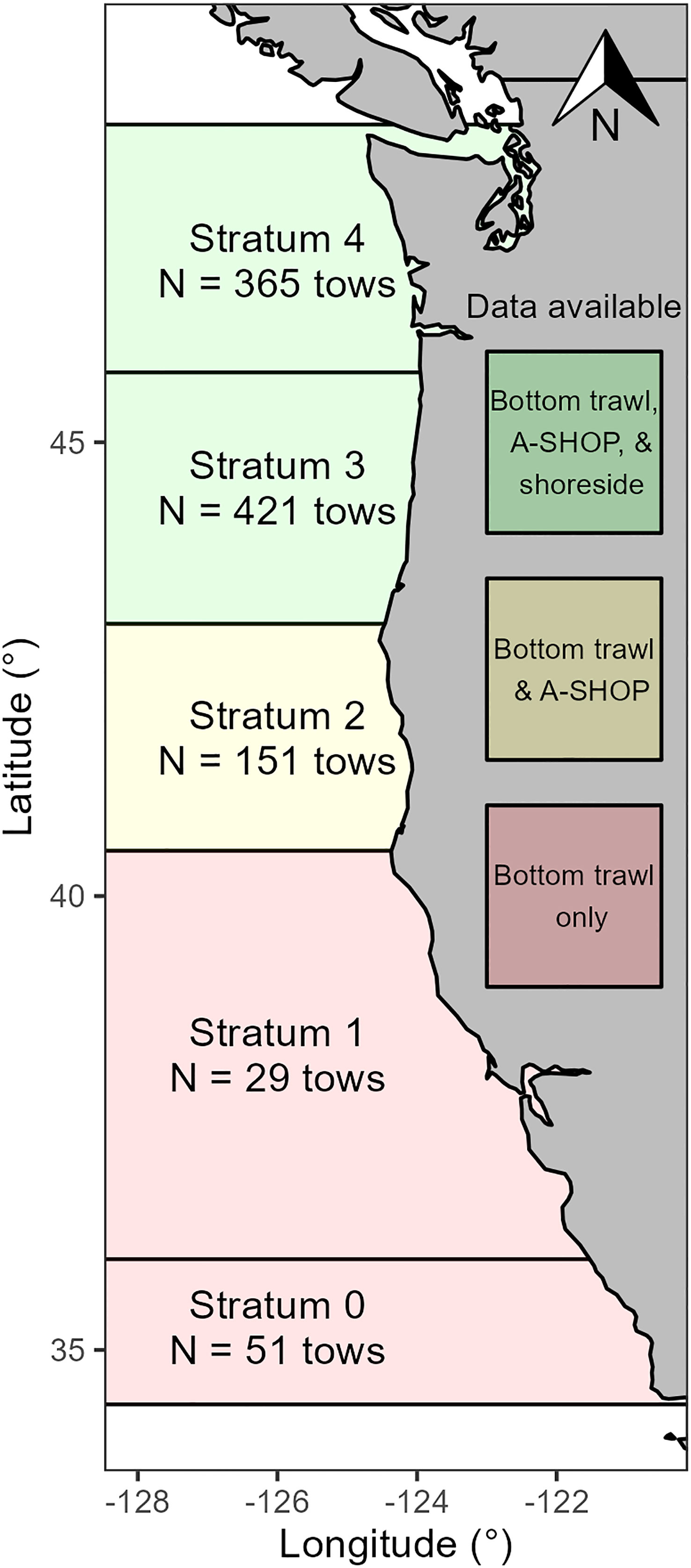
Figure 1 Study area with International Pacific Fisheries Commission Geographic Strata (0-4), type of data generally available in each stratum, and number of tows by strata for 2019. A-SHOP refers to at-sea hake observer program data, shoreside refers to the hake fishery in which catches are processed on shore, and bottom trawl refers to the NOAA Northwest Fisheries Science Center fishery-independent bottom trawl survey. We note that while the figure depicts the general lack of shoreside data in stratum 2, 4 shoreside tows were conducted in stratum 2 across years and included in this study.

While 2019 was the focal year of this study as it was the year in which the USV survey was conducted in tandem with the ATS, we also analyzed data from previous years in which the ATS was conducted using modern protocols (i.e., protocols that closely resemble current protocols; 2003, 2007, 2009, 2011, 2012, 2013, 2015, and 2017). We did this to examine the performance of our method for generating estimates of hake age composition with a STM fit to non-contemporaneous biological sampling data under different stock population structures (age composition, size/status, and distribution).

2.2 Acoustic trawl survey and data processing

The U.S. portion of the 2019 ATS began near Point Conception, California and proceeded north along the west coast of the United States to the Canadian border. Acoustic transects were oriented east-west and ranged from the 50 m isobath to either the 1,500 m isobath or a location 35 nmi west of the inshore waypoint. Transects were spaced 10 nmi apart. Transects were traversed sequentially and were surveyed acoustically between sunrise and sunset when hake form identifiable aggregations. A Simrad scientific echosounder system collected raw acoustic data from up to five split-beam transducers operating at 18, 38, 70, 120, and 200 kHz (pulse duration: 1 ms; ping rate: 1-4 per second depending on bottom depth). Echosounder calibrations were performed pre- and post-survey according to standard procedures (Demer et al., 2015). Data from the 38 kHz echosounder (the primary frequency used for generating biomass estimates) were post-processed for hake based on scattering properties and behavioral cues (e.g., school morphology; see Supplementary Material S1 and Chu et al. (2017) for further details on echogram scrutiny). Daytime trawling was used to classify observed backscatter layers to species and size composition and to collect specimens of hake and other organisms (see Supplementary Material S1 and Chu et al. (2017) for further details on calculation of hake backscatter in mixed aggregations). The number and locations of trawls were not pre-determined, but instead depended on the occurrence and pattern of backscattering layers observed at the time of the survey. Highest priority for trawling was given to sampling distinct layers of intense backscatter that are indicative of high densities of hake. While southern and offshore extents, transect spacing, and acoustic frequencies employed (namely, the inclusion of 18 kHz) varied moderately over the study period (2003-2019), the purpose of the ATS (generating a biomass index for the hake stock) and core methodology remained constant. Notably, the ATS biomass estimates did not include INPFC stratum 0 in 2003-2011, and no biological data were collected in stratum 0 in 2003-2007.

2.3 Saildrone (USV) survey and data processing

The U.S. portion of the 2019 ATS was conducted on the fishery survey vessel (FSV) Bell M. Shimada and ran from June 15 to August 21, with concurrent survey operations by four to five USVs (Saildrones from Saildrone, Inc.) operating from June 17 to August 25. The USVs were equipped with the company’s standard package of oceanographic and atmospheric sensors, including Simrad scientific echosounders mounted in the USV’s keelpod. The echosounder system consisted of an EK80 Wide Band Transceiver Mini with a 38 kHz split beam transducer and a 200 kHz single beam transducer (ES38-18/200-18C; pulse length: 1.024 ms; ping rate: 1 per two seconds). Echosounder calibrations were performed pre- and post-mission (June 10 and September 27, respectively) off the Saildrone, Inc. dock in Alameda, CA according to standard procedures (Demer et al., 2015).

At-sea operations of the USVs were governed in two ways. Pre-mission planning of sampling protocols established mission parameters at the outset (for example, only surveying acoustically from sunrise to sunset). In-field decisions based on navigation and weather data delivered via a graphical user interface (the mission portal), were operationalized through near real-time satellite-driven command and control of the vessel’s navigation. USV operators – all pilots and engineers employed by Saildrone, Inc. – piloted the vessels in collaboration with NWFSC scientists aboard the research vessel monitoring the USVs through a web-based mission portal.

The USVs surveyed the same parallel transects as the ATS in the same direction along the U.S. west coast, from south to north. Each transect was either surveyed entirely by one USV, or by a pair of USVs operating in conjunction to cover either the inshore or offshore halves. This practice of using multiple USVs for a single transect helped mitigate the difference in operational speed between the USVs and the research vessel. In the 2019 mission, the USVs matched the FSV in completing 85 transects over their 70 operational days. USV survey speeds varied across the five vehicles, depending on weather, currents, and operational idiosyncrasies inherent to each vehicle. In general, the speed-over-ground for the USVs ranged from 0 knots when becalmed, to nearly 5 knots when transecting in 20 plus knots of wind from favorable directions. In the three instances where the ATS protocol extended a transect to follow suspected hake backscatter (hake designation methodology briefly explained below, and in further detail in Supplementary Material S1 and Chu et al. (2017)), the USVs likewise extended. Operationally, 68% of the USV transects were within +/- 3 days of the ATS transects, while 84% were within +/- 5 days.

The post-cruise judging team for the USV transects used Echoview 11 (a commercial software developed by Echoview Software Pty.; https://echoview.com). The team was organized to minimize initial recollection bias from any FSV echograms they might have viewed in the previous cruise legs. This was done by tasking two analysts to judge those USV transects where they themselves had not also been on board the ATS when the ship sampled those particular lines. Furthermore, these analysts did not review the archived trawl or processed acoustic data from these ATS transects prior to reviewing the ATS collections in their charge. Lastly, a procedural, final review of all echograms by the survey’s chief scientist, though conducted for the ATS echograms, was withheld from the USV echograms.

Insofar as possible, given the lack of validating trawl data and the reduced number of acoustic frequencies available for the USVs versus the ATS (38 and 200 kHz versus the 18, 38, 70, 120, and 200 kHz), acoustic data review was done in a similar fashion to that of the ATS judging. The “Impulse Removal” and “Background Noise Removal” processing modules within Echoview software were used for the 38 and 200 kHz echograms, to better account for signal attenuation from inclement weather. The 38 and 200 kHz echograms were scrutinized simultaneously, with identifying regions drawn around suggestive backscatter in the 38 kHz echogram. Regions drawn in one echogram automatically appear in all others, allowing comparisons. In drawing regions, analysts relied on morphometric cues (shape, size of the aggregations), behavioral cues (depth, relative positioning to other schools, proximity to the 200-meter shelf break), and frequency response (when possible), to make their determinations.

Regions were drawn tightly around areas judged as likely to be “hake” (i.e., 100% hake), “CPS” (i.e., coastal pelagic species), “zooplankton,” or “unclassified.” Unlike with ATS judging, no species mixes or biological information was linked for these regions. In most instances determined to be hake, judges relied on the evidence offered by the 38 kHz alone, as hake typically occurs at depths greater than range of good data from the 200 kHz. Lastly, the two USV reviewers met after all assigned transects were completed to hold their own procedural review. Each EV file was jointly scrutinized so as to make a shared, consistent decision about the shape and assignation of each backscatter region within. Supplementary Material S1 and Chu et al. (2017) provide further detail on echogram scrutiny.

2.4 Biological data for spatio-temporal models

STMs were fit to data from three sources: the NWFSC’s Pacific Coast Groundfish Bottom Trawl Survey (hereafter ‘bottom trawl’), the At-Sea Hake Observer Program (‘A-SHOP’), and observer data from each state’s shoreside hake fishery (i.e., fishery in which catches are processed on shore; ‘shoreside’). We describe these data briefly below.

Bottom trawl data were available across the study area from May-October in each year of the study, and were collected at random sites across the U.S. West Coast at depths from 55-1,280 m from chartered fishing vessels (Keller et al., 2017). There were 164 tows in 2019 and 2,140 tows across all years that were retained for analysis. Sites were selected via a stratified random grid-based design in which percentages of sampling effort were allocated to each INPFC geographic stratum (Keller et al., 2017). Tows were conducted on trawlable habitat within the selected grid cell for 15 minutes (plus liftoff lag, Wallace and West, 2006) and catch weights were recorded for each species caught. A subsample of hake in each trawl was weighed, measured, and later aged. We allocated total hake weight by age class for each haul based on the age class proportions recorded in the haul’s subsample and overall median weight-at-age-class from all hauls across the survey area.

A-SHOP data were available in INPFC strata 2-4 (Figure 1) in each year in May, June, September, October, and November, although some years had data from July and August as well (n = 284 tows in July and August across years). There were 775 tows in 2019 and 5,323 tows across all years that were retained for analysis. These data were recorded by National Marine Fisheries Service (NMFS) observers aboard at-sea processing vessels (catcher-processors and motherships) that generally fish offshore of Oregon and Washington but occasionally set nets in Northern California (catcher motherships only). Observers recorded the haul weight for each species observed and a subsample of hake in each trawl was weighed, measured, and then later aged by shore-based personnel (NWFSC, 2022). In the same manner as the bottom trawl data, we allocated total hake weight by age class for each haul based on the age class proportions recorded in the haul’s subsample and overall median weight-at-age-class from all hauls across the survey area.

Shoreside data were generally available in INPFC strata 3-4 (Figure 1) in each year of the study from May-October, and were recorded by NMFS observers aboard fishing vessels that deliver their catch to shore-based processing plants. Only a very small number of tows (n = 4 across years) were conducted south of stratum 3 (i.e., in stratum 2). There were 69 shoreside tows in 2019 and 476 tows across all years that were retained for analysis. Shoreside vessels generally fish offshore of Oregon and Washington but often at closer distances to shore than at-sea vessels (Saelens and Jesse, 2007). Observers recorded the haul weight of each species observed and a subsample of hake from each trip was weighed, measured, and later aged. Because hake were subsampled onshore after trips were completed, and more than one haul was conducted on some trips, it was necessary to assign age class compositions to the centroid of the broader area that was fished on a given trip by a given vessel. After this was done, we allocated total hake weight by age class for each haul based on the age class proportions recorded in the haul’s subsample and overall median weight-at-age-class from all hauls across the survey area in the same manner as the other data sources.

2.5 STM specifications and age class proportions

Spatially and temporally resolved estimates of hake biomass-at-age class, which were subsequently converted to proportions of biomass at age class, were derived from STMs built with the VAST R package (ver. 3.7.1; Thorson and Barnett, 2017) in the R Studio environment (R ver. 4.04). We provide an overview of our VAST-based STMs here but refer the reader to Thorson (2019) for additional details about VAST models in general. Our STMs were configured to make predictions over three groups of months: May-June, July-August, and September-November. These delineations were made based on data availability and to capture the seasonal northward migration of hake (Hamel et al., 2015). For 2019, we employed a 3x3 factorial design with three age class configurations (three, four, and five age classes; Table 1) and three configurations for spatial and spatio-temporal terms (independent, identically distributed factors (IID), single-factor, multi-factor; Table 2). For the other study years, we employed a 3x1 factorial design and tested the three model term configurations with the age class configuration that performed best in 2019. Age class configurations were chosen based on hake life history (e.g., differences in weight-at-age, scale of migration between ages), available data, and the distribution of samples in 2019. Candidate age class configurations differed in the resolution of older adult (age 4 and older) ages (Table 1), which was limited given that data availability declined with age. Model term configurations were chosen to represent situations in which the spatio-temporal biomass distribution of age classes (1) varied independently from one another (IID configuration), (2) was affected by the same spatial and spatio-temporal variables (single-factor configuration), or (3) was affected by multiple spatial and spatio-temporal variables at different levels of impact between age classes (multi-factor configuration) (Table 2).

TABLE 1

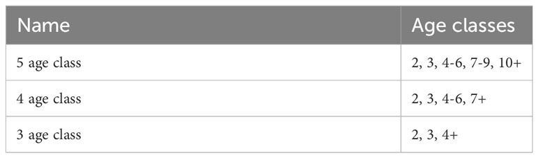
Table 1 Candidate STM age class configurations.

TABLE 2

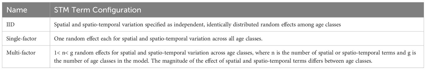
Table 2 Candidate STM term configurations.

Specifically, STMs fit in the VAST R package were developed using a delta generalized mixed model framework. We describe the models by starting with the basic formulation of temporal, spatial, and spatio-temporal effects and building to the incorporation of a spatially-varying catchability term and the alternative incorporation of effects via model term configurations. Linear predictors for encounter/non-encounter (p₁) and biomass conditional on encounter (p₂) for age class $c_i$, month group $t_i$, and spatial knot $s_i$ were each defined as follows:

Eq. 1,

$$p(i)= \beta (c_i,t_i)+ \omega (s_i,c_i)+ ϵ(s_i,c_i,t_i)$$

where $\beta$ is a fixed effect for temporal variation (month group). Spatial ($\omega$) and spatio-temporal ($ϵ$) variation were modelled as random effects with a first-order autoregressive correlation structure between month groups. Since we fit the model to a combination of fishery-dependent and fishery-independent data, it was necessary to add a catchability ratio to the model to account for differences in fishing power between datasets (Thorson et al., 2012; Grüss et al., 2023). We specified the catchability ratio as a spatially-varying effect because spatial domain and selectivity at age can vary between fishery-independent and fishery-dependent data (Grüss et al., 2023; Thorson et al., 2023). Additionally, hake spatial distribution is known to vary with age (Hamel et al., 2015). With the addition of a spatially-varying catchability ratio in each linear predictor, the formulation becomes:

Eq. 2,

$$p(i)= \beta (c_i,t_i)+ \omega (s_i,c_i)+ ϵ(s_i,c_i,t_i)+\underset{\sum }{\overset{}{}}\underset{m=1}{\overset{n_m}{}}\xi (s_i,m)M(i, m)$$

where $\xi (s_i,m)$ is is the additive, spatially-varying impact of data source $m$ at location $s_i$. This impact is set to 0 for the fishery-dependent data and is estimated for the fishery-independent data as a random effect following a multivariate normal (MVN) distribution:

Eq. 3

$$\zeta (i)\sim \text{MVN}(\lambda 1,{\sigma }_{\lambda }^2(m)R(k))$$

where $\lambda 1$ is a matrix of fixed effects (average log-ratio between fishery-dependent and fishery-independent data), ${\sigma }_{\lambda }^2$ is the estimated pointwise variance of the spatially varying response to fishery-dependent data m, and R is a matrix of spatial correlations given an estimated decorrelation distance k. Because the spatially-varying data source effect is set to 0 for the fishery-dependent data, it then follows that the specified spatially-varying data source effect on expected catch rates enables the estimation of a fishing-power ratio for the fishery-independent data relative to the fishery-dependent data. Fishery-dependent data were set as the ‘reference’ data because of (1) relative similarity in fishing practices between the fishery and ATS when compared to the non-target fishery-independent bottom trawl data and (2) richness (i.e., number of observations, spatial and temporal coverage) of the fishery-dependent data relative to the non-target fishery-independent bottom trawl data.

Eq. 2 was the final formulation for the ‘IID’ model term configuration, in which the distribution of hake within age classes varies independently from other age classes. In the ‘single-factor’ model configuration, we included loading vectors L to add the correlation of single spatial and spatio-temporal effects between age classes:

Eq. 4,

$$p(i)=\beta (c_i,t_i)+L_{\omega }(c_i)\omega (s_i)+L_{ϵ}(c_i)ϵ(s_i,t_i)+\underset{\sum }{\overset{}{}}\underset{m=1}{\overset{n_m}{}}\xi (s_i,m)M(i,m)$$

In the ‘multi-factor’ model configuration, we must sum across multiple spatial and spatio-temporal random factors f to capture the aggregate spatial and spatio-temporal effects, and the loading vector L becomes a matrix with dimensions n_c × $n_f$:

Eq. 5,

$$p(i)= \beta (c_i,t_i)+ \underset{\sum }{\overset{}{}}\underset{f=1}{\overset{n_{\omega }}{}}{L}_{\omega }(c_i,f)\omega (s_i,f)+\underset{\sum }{\overset{}{}}\underset{f=1}{\overset{n_{ϵ}}{}}{L}_{ϵ}(c_i,f)ϵ(s_i,f,t_i)+\underset{\sum }{\overset{}{}}\underset{m=1}{\overset{n_m}{}}\xi (s_i,m)M(i, m)$$

In some cases, the variance or effect of spatial and spatio-temporal terms approached zero. These terms were iteratively removed such that the final models contained only terms with quantifiable, non-zero effects and variances. In the multi-factor configuration, the number of factors $n_f$ in the initial model was set equal to the number of categories $n_c$. To ensure that only influential predictors were retained in the final model, models were re-fit iteratively after removing factors with proportions of explained variance, as estimated in the loadings matrix, lower than 10%.

In all models, a gamma distribution was specified for the error of the second linear predictor. All models employed 500 spatial knots, which provided a suitable balance between resolution and run times based on preliminary analyses. It was not possible to directly include an effort offset due to incomplete recording of effort metrics across datasets. For this stock, it is common practice to assume biological sampling effort from at-sea vessels (tows) and shoreside vessels (trip) are approximately equivalent (Berger et al., 2023).

Each linear predictor was transformed using a conventional logit or exponential power link function to predict sample data as follows:

Eq. 6,

$$r_1(i)=logi{t}^{-1}(p_1(i))$$

$$r_2(i)=exp(p_2(i))$$

where the subscripts 1 and 2 indicate encounter/non-encounter and biomass conditional on encounter, respectively.

A probability density function to predict biomass density B was specified as:

Eq. 7,

$$f(B= b_i)= {\{}_{r_1(i)\ast Gamma\left\{B=b_i|r_2(i),{\sigma }_m^2(c_i)\right\} if B>0}^{1-r_1(i) if B=0}$$

where $b_i$ is biomass density for sample i, ${\sigma }_m^2(c_i)$ is the residual variance in positive catch rates, and $f(B= b_i)$ is the data likelihood function.

Given the above, biomass density ( $d(s,c,t)$) was predicted for each location, category, and time by transforming linear predictors and removing terms that affect catchability:

Eq. 8,

$$\begin{array}{l}d(s,c,t)=logi{t}^{-1}({\beta }_1(c_i,t_i)+{\displaystyle \sum _{f=1}^{n_{\omega 1}}{L}_{\omega 1}(c_i,f){\omega }_1}(s_i,f)+{\displaystyle \sum _{f=1}^{n{n}_{ϵ1}}{L}_{ϵ1}(c_i,f){ϵ}_1}(s_i,f,t_i))\\ \ast exp({\beta }_2(c_i,t_i)+{\displaystyle \sum _{f=1}^{n_{\omega z}}{L}_{\omega 2}(c_i,f){\omega }_2}(s_i,f)+{\displaystyle \sum _{f=1}^{n_{ϵz}}{L}_{ϵ2}(c_i,f){ϵ}_2}(s_i,f,t_i))\end{array}$$

in all cases, biomass density estimates were corrected for retransformation bias using the epsilon estimator (Thorson, 2019).

Proportions at age-class (i.e., age class compositions) were calculated by dividing the biomass estimate for a given age class by the overall biomass estimate across age classes at each location and time point. We used this proportion at age class estimate as an input to the standard ATS biomass estimation process (a replacement for proportions at age measured with biological sampling in the ATS), which also incorporates acoustic data and is described in a subsequent section. Since STM biomass estimates were not derived from acoustic data and were only used to calculate proportion-at-age class, we did not draw any conclusions from the STM biomass estimates themselves.

2.6 Comparisons between age composition estimates

After proportional age class compositions were calculated from STM biomass-at-age class predictions, they were compared with observed proportional age class compositions from the ATS across the study area, within INPFC geographic strata (Figure 1), and across the area in which fishery-dependent data were available (INPFC strata 2-4). Comparisons were made in each of the study years. Notably, the ATS did not sample INPFC stratum 0 in some years (2003, 2007), so statistics reported for stratum 0 are based on fewer years than statistics in other strata. The model configuration that produced age class composition estimates that were most similar to age class composition observations from the ATS in 2019 was selected for use in biomass estimation.

Differences in age class compositions were represented as both the average absolute difference in proportion-at-age class (across strata, age classes, or both) and median relative error, which was calculated by

Eq. 9,

$$\frac{p_{ATS}-p_{STM}}{p_{ATS}}*100$$

Where $p_{ATS}$ is the proportion at age class observed in the ATS and $p_{STM}$ is the proportion at age class estimated by the STM. Relative error was represented with a median value rather than a mean as infinite values were calculated when the ATS proportion-at-age-class was zero.

2.7 Biomass estimation and comparisons

For biomass estimation, it was necessary to refine age class compositions derived from STMs (Table 1) into exact age compositions. For each stratum, the STM-estimated proportion at age class was multiplied by the proportion of exact ages within that age class, as calculated from the raw model input data (A-SHOP, shoreside, and bottom trawl). Empirical weight-at-length and weight-at-age relationships were also calculated from raw model input data across the entire survey area for biomass calculations.

To be consistent with the standard ATS biomass estimates, biomass estimates for age-2 and older hake were calculated using standard procedures in the ATS (Chu et al., 2017), with three notable exceptions: 1) biomass estimates were generated with INPFC geographic strata instead of with strata developed within the ATS procedure based on similarity in trawl composition, 2) biomass was only estimated in U.S. waters (excluding Alaska; not the full extent of the stock into Canadian waters), and 3) the ATS age composition had age-1 hake removed prior to the biomass calculation. Therefore the acoustic backscatter that would have been converted to age-1 hake under standard protocols was instead allocated to age-2 and older fish, since it was not possible to differentiate age-1 hake from 2 and older hake in the USV dataset due to the lack of contemporaneous biological sampling. Age-1 hake are treated in a multi-factor manner by the survey and inclusion would confound the results.

Briefly, acoustic backscatter attributed to hake was apportioned based on age composition data, scaled to biomass using the hake target strength-length relationship (Traynor, 1996) and empirical weight-length and weight-age relationships, then kriged over the study area to generate a biomass estimate resolved by space and age (Chu et al., 2017). We note that the biomass estimates presented in this study differ from those used in the stock assessment for management of hake due to the differences described above, and caution against the use of biomass estimates presented in this study for anything other than a research purpose.

For all years, we estimated biomass-at-age with 38 kHz acoustic data collected in the ATS paired with (1) age compositions from the ATS, and (2) age composition estimates from a STM. Based on preliminary observations of poor STM performance in stratum 0, we also estimated biomass-at-age with age composition estimates from the best STM for strata 1-4 paired with an average age composition from the ATS in stratum 0 (across study years, 2009-2019, excluding the estimation year) as a sensitivity analysis. Results for this sensitivity analysis were presented in Supplementary Material S2. For 2019, we generated biomass estimates by pairing the three sources of age composition data described above with two sources of 38 kHz acoustic data: 1) the ATS, and 2) the USV. In the main text, we report comparisons between total biomass estimates derived from different combinations of data. We report biomass-at-age estimates derived from each combination of data in Supplementary Material S3.

Differences in total biomass estimates derived from STM age composition estimates and observed ATS age composition data were qualitatively examined to investigate the robustness of results at different life-stages and population structures. This was a qualitative analysis given the low number of study years and high number of plausible influential factors.

2.8 Model evaluation

To further evaluate models fit to 2019 data, we conducted simulation testing and k-fold cross-validation procedures. Here, we note that although the operational product of the STMs was a biomass-at-age class composition (proportion), the models themselves predicted biomass-at-age class (from which we subsequently calculated age class proportions). So, model evaluations were conducted with biomass-at-age class estimates as response variables, which have substantially higher dimensionality than age class composition estimates. Given the indirect nature of these evaluation procedures, we presented further details and results in Supplementary Material S4.

3 Results

3.1 Comparisons between ATS and STM age compositions

In 2019, The 5-age class model configuration (Table 1) produced estimates of age class composition that were most similar to observed age class compositions from the ATS (see Supplementary Material S5 for results from other age class configurations). Differences between model term configurations were small in 2019. Across the study area, the average absolute difference in proportion-at-age class was 0.09 (median relative error: 19.45%) for the single-factor model configuration, and 0.11 for the multi-factor and IID model configurations (median relative errors: 26.50, 26.76%, respectively). In the areas where both fishery-dependent and fishery-independent data were available (INPFC strata 2-4), the average absolute difference in proportion-at-age class was 0.03 (median relative error: 11.46%) for the single-factor model configuration, 0.04 (median relative error: 15.77%) for the multi-factor configuration, and 0.05 (median relative error: 15.85%) for the IID configuration. The single-factor term configuration of the 5-age class model was therefore selected for further examination and biomass estimation. We refer to this model configuration as the ‘best STM’ hereafter. Proportion at age class values for other term configurations of 2019 STMs and the 2019 ATS by strata were reported in Supplementary Material S6.

In 2019, the best STM produced age class compositions that were most similar to observed age class compositions in the ATS in stratum 2 (Figure 2). Predicted proportions at age class in strata 1, 2, 3, and 4 were all within 0.07 (median relative errors: 52.79, 6.03, 12.02, 19.45%, respectively) of proportions in the ATS across age classes, while differences in proportions across age classes in stratum 0 exceeded 0.3 (median relative error: 546.29%) (Figure 2). The high magnitude of differences in stratum 0 were driven by proportions of age-2 hake in the ATS data that exceeded 0.9, which no model configuration was able to predict (Figures 2, S4.2; S4.3).

FIGURE 2

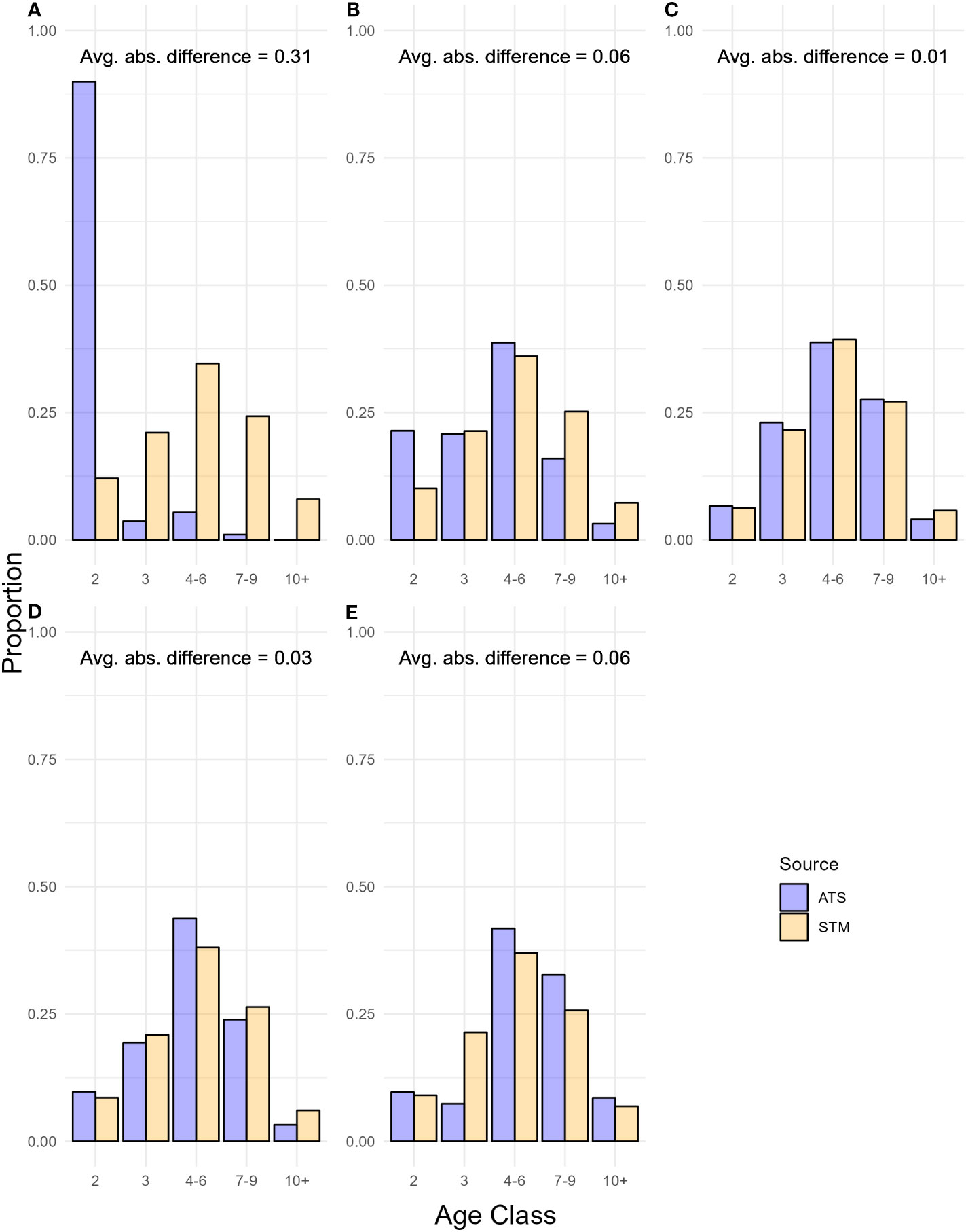
Figure 2 Age class composition in 2019 from the best spatio-temporal model (STM) predictions and hake acoustic-trawl survey (ATS) data in (A) INPFC stratum 0, (B) stratum 1, (C) stratum 2, (D) stratum 3, and (E) stratum 4. Avg. abs. difference refers to the average absolute value of differences between STM and ATS age compositions across age classes.

Across study years,the single-factor 5-age class model produced estimates of age composition that were slightly more similar to ATS observations than other term configurations (Supplementary Material S7), validating our designation of the single-factor 5-age class model as the best STM. Detailed comparisons in individual years other than 2019 for all term configurations were presented in Supplementary Material S8. Across the entire study area and time period, the average difference in proportion-at-age class between the best STM and the ATS was 0.14 (median relative error: 79.03%; Figure 3). In the area where both fishery-dependent and fishery-independent data were available (INPFC strata 2-4), the average difference was 0.09 (median relative error: 54.96%; Figure 4). Relative error in proportion-at-age class estimates were highest and most variable for older age classes (7-9, 10+, Figures 3, 4), likely due in part to low relative abundance magnifying slight deviations in proportion-at-age estimates. On average, the best STM produced estimates of age class composition that were most similar to observed age class compositions in the ATS in strata 3 and 4 (0.08 average absolute difference; median relative errors: 61.1, 44.1%, respectively). The average absolute difference in proportion at age class across age classes and years was 0.11 (median relative error: 68.84%) in stratum 2, 0.16 (median relative error: 79.55%) in stratum 1, and 0.26 (median relative error: 510.27%) in stratum 0. Similar to results in 2019, the high magnitude of differences in stratum 0 across years was driven by high proportions of age-2 hake in ATS data – in some years representing 100% of the catch – which no model configuration was able to replicate. We note that the ATS did not collect biological samples in stratum 0 in 2003 and 2007, so results presented above for stratum 0 are based on fewer years than other strata.

FIGURE 3

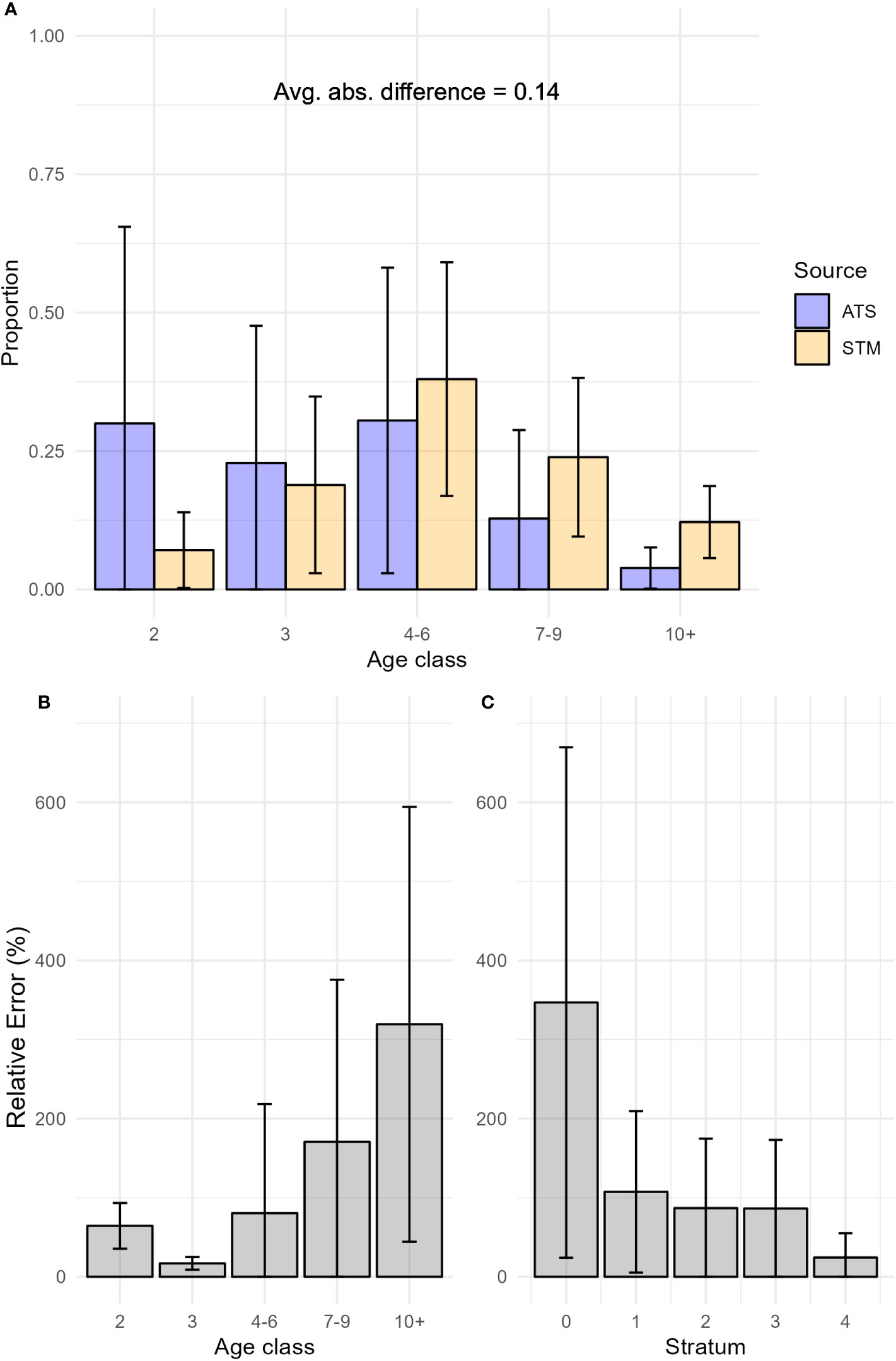
Figure 3 (A) Proportion at age class from the best spatio-temporal model (STM) model predictions and the hake acoustic trawl survey (ATS) data from 2003-2019, (B) Average relative error of STM proportion at age class predictions by age class from 2003-2019, and (C) Average relative error of STM proportion at age class predictions by strata from 2003-2019-. Bars indicate the standard deviation of the quantity plotted. Avg. abs. difference refers to the average absolute value of differences between STM and ATS age compositions across age classes.

FIGURE 4

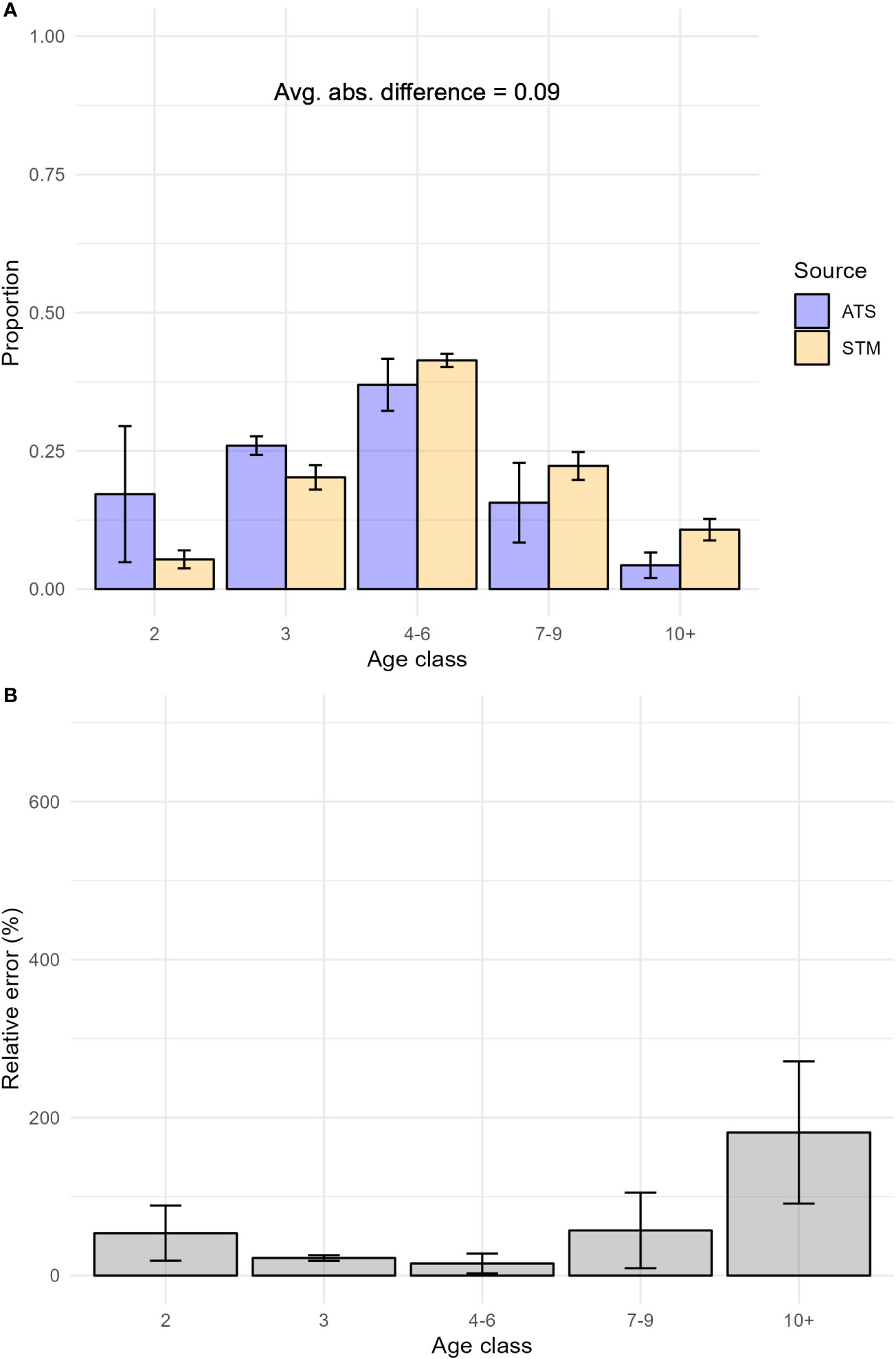
Figure 4 (A) Proportion at age class from the best spatio-temporal model (STM) model predictions and the hake acoustic trawl survey (ATS) data from 2003-2019 in strata 2-4, and (B) Average relative error of STM proportion at age class predictions by age class from 2003-2019 in strata 2-4. Bars indicate the standard deviation of the quantity plotted. Avg. abs. difference refers to the average absolute value of differences between STM and ATS age compositions across age classes.

3.2 Comparisons between biomass estimates

For 2019, changing the source of acoustic data (ATS or USV) used for biomass estimation had a nearly ten-fold higher impact on biomass estimates than changing the source of age composition data (ATS or STM) (Table 3). Total biomass estimates were not substantially impacted if ATS average age compositions were substituted for STM predictions in stratum 0 (Supplementary Material S2). For 2019, holding the source of age composition constant and changing the source of acoustic data for biomass estimates yielded differences in biomass of 22.4% (when STM age compositions were used in both cases) and 26.8% (when ATS age compositions were used in both cases), while holding the source of acoustic data constant and varying the source of age composition data yielded differences in biomass of 2.6% (when USV acoustic data were used in both cases) and 3.2% (when ATS acoustic data were used in both cases) (Table 3).

TABLE 3

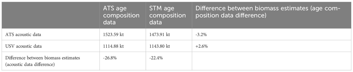
Table 3 Total hake biomass estimates (kilotonnes; kt) derived from different sources of data in 2019.

Overall, the average difference between biomass estimates derived from ATS and STM age composition data was 5.6% (7.2% absolute difference). Differences between biomass estimates derived from ATS and STM age composition data were least pronounced in 2003, 2013, and 2019 (-3.9%, 2.4%, and -3.4%, respectively; Figure 5). Differences were between 7.2% and 11.1% in 2007-2012, 2015, and 2017 (Figure 5). From 2007-2017, biomass estimates derived from STM age composition estimates exceeded estimates derived from the observed ATS age composition data, while less biomass was estimated in 2003 and 2019 (Figure 5). Differences between biomass estimates derived from STM age composition estimates and observed ATS age composition data appeared to be qualitatively associated with population structure (i.e., total biomass and the proportion of young, maturing age-2 and 3 hake in the ATS biological sampling; Figure 5). With notable exceptions, biomass estimates derived from STM age composition estimates were most comparable to those derived from observed ATS age composition data when the proportion of age-2 and 3 hake were low and total hake biomass was high (Figure 5).

FIGURE 5

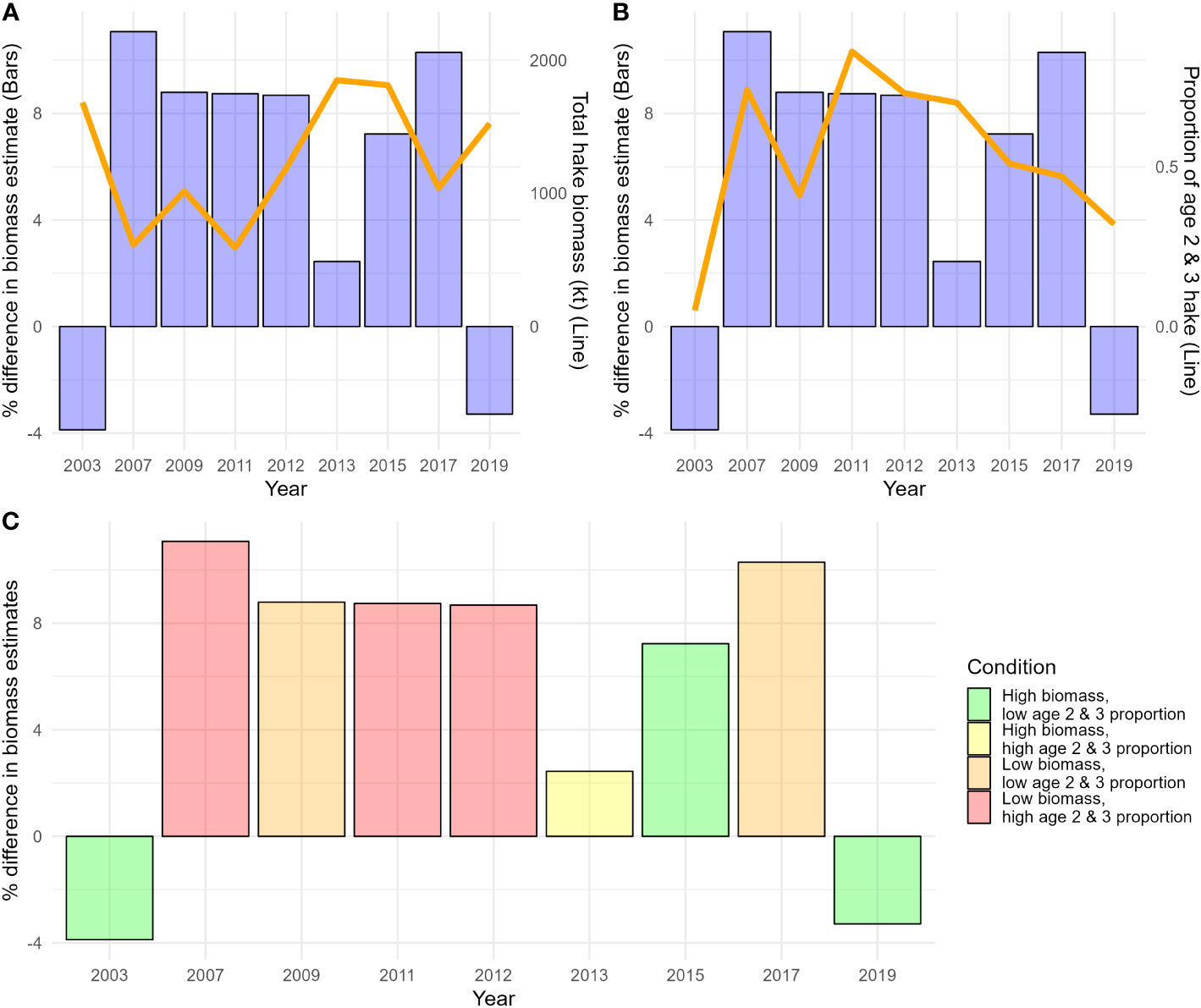
Figure 5 Differences in total biomass estimates derived from the best spatio-temporal model (STM) age composition estimates and observed hake acoustic trawl survey (ATS) age composition data across years. (A) Percentage difference in biomass estimates (bars) and total age-2 and older hake biomass (line). Percentages reflect differences in biomass estimates derived from ATS only (age composition and acoustic) and STM predictions (age composition) paired with ATS acoustics relative to ATS biomass estimates. (B) Same as A, but with the proportion of age-2 and 3 hake sampled in the ATS (line). (C) Same as A, but years are color coded according to different population structure conditions: high or low total biomass and biomass of young, maturing (age 2 and 3) fish. Low and high were demarcated by the overall average (biomass: 1256.93 kt; age 2 and 3 proportion: 0.53).

4 Discussion

The inability of USVs to collect biological composition data (e.g., age, length) has thus far hampered their use in fishery resource survey programs. We developed an approach that utilizes non-contemporaneous biological sampling data (a combination of fishery-dependent and non-target fishery-independent data) fit to a STM to address this limitation. In the areas where fishery-dependent data were available (INPFC strata 2-4; Figure 1), this approach produced estimates of proportional age class composition that were on average within 0.03 of proportional age class compositions observed in the hake ATS in the study focal year of 2019 (median relative error: 11.46%), and 0.09 on average across the study period (2003-2019; median relative error: 54.96%) (Figures 2, 3). While the magnitude of differences between modelled and observed age compositions was greater across the entire study area (0.09 difference on average in 2019, median relative error: 19.45%; 0.14 difference on average across all years over the entire survey area, median relative error: 79.03%), total biomass estimates that were derived from STM age composition estimates were within approximately 7% of those derived from ATS composition data given the same source of acoustic data across study years (~ 3% in 2019; Table 3). These levels of change in the overall survey biomass estimate are well below the total variability (coefficient of variation of 36%) associated with the ATS in recent stock assessments (Berger et al., 2023). While differences between STM- and ATS-produced age compositions did not translate into large discrepancies in total biomass, accurate estimates of age structure remain particularly important for management operations. In particular, age-2 and 3 compositions in the most recent survey provide a critical first observation related to recent recruitment levels for the stock assessment, and recent recruitment estimates considerably impact current and near-term harvest specifications for Pacific Hake. Future work should evaluate how alternative survey protocols ultimately influence existing management procedures (e.g., stock assessment formulation and harvest policy) by integrating specific results from this work into the existing Pacific Hake management strategy evaluation tool (Jacobsen et al., 2021).

When biomass was estimated from USV (Saildrone) acoustic data, estimates differed from those derived from ATS acoustic data by more than 22%, regardless of whether STM or ATS age composition information was used (Table 3). Thus, the primary limitation for operationalizing USV data for hake biomass-at-age estimation appears to be rectifying discrepancies between USV and ATS acoustic data, whereas the lack of contemporaneous age composition sampling associated with USV surveys appears secondary. There are several explanations for the differences between acoustic backscatter recorded by USVs and the acoustic backscatter recorded by the ATS in this study. The most prominent of those include signal attenuation due to bubble injection (Simmonds and MacLennan, 2005; Shabangu et al., 2014; Ryan et al., 2015), other effects of inclement weather, which are more pronounced for USVs (Jech et al., 2021), calibration uncertainty (Demer et al., 2015; De Robertis et al., 2019a), differences in vessel response (De Robertis and Handegard, 2013; De Robertis et al., 2019b), and differences in the ability of analysts to identify hake from other species in acoustic data. The final consideration is one of the most plausible source of the observed differences in backscatter, as while there are well-established procedures for identifying hake in acoustic data, analysts of USV data made most determinations based on 38 kHz data alone (or with limited information from 200 kHz) rather than based on several frequencies (18, 38, 70, 120, 200 kHz) and in conjunction with trawl data.

Biological sampling is crucial for ground-truthing acoustic surveys. While we showed that reasonable age compositions can be estimated for hake without it in some areas, contemporaneous biological sampling remains the most viable method for validating estimated species compositions in the ATS. The lack of biological data for analysts to verify species classifications in the acoustic data and the limited suite of acoustic frequencies available led to more subjective designations by analysts. Results indicated that the increased subjectivity led to analysts taking a precautionary approach to apportioning backscatter to hake. The high relative importance of biological sampling and multiple frequencies in the ATS echogram judging procedures may be reflected by comparing our findings with others who compared research vessel and USV data. We observed substantially less hake backscatter in USV data relative to research vessels, while others observed more backscatter in USV data (Swart et al., 2016; Chu et al., 2019; De Robertis et al., 2019b). Given the performance of STMs for estimating age compositions and the capability for other USVs to be equipped with a suite of echosounders that are more comparable (or exactly the same) to the research vessel suite, reliably classifying acoustic backscatter by species is the most significant obstacle to using USV data to produce viable biomass-at-age estimates. It is possible that STMs fit to fishery and non-target fishery-independent data could be useful in overcoming this obstacle. However, automated methods for species classification in acoustic data (e.g., artificial intelligence/machine learning, Sarr et al., 2021; inversion methods, Urmy et al., 2023) and analysis of frequency modulated (i.e., broadband) acoustic data are likely to have the most utility.

Using STMs to provide age composition data worked reasonably well because of an important property of the data we used to fit our models and hake survey protocols. In general, fishers target larger, older individuals (Birkeland and Dayton, 2005). However, the boom-and-bust nature of hake recruitment results in the stock being supported primarily by two-to-four strong age classes in any given year (Horne and Smith, 1997; Hamel et al., 2015; Johnson et al., 2021). As a result, hake fishers target the larger and older hake less than they would if fishing a species with more constant recruitment. This means that differences in selectivity at age between fishery-dependent and fishery-independent data are not pronounced – at least for hake older than three (Figure S9.1; Berger et al., 2023). Further, the ATS does not trawl randomly along survey transects and instead targets suspected aggregations of hake. Thus, trawling locations in the ATS are decided using criteria that are largely similar to those the fishery uses, although the diffuse aggregations of hake are likely targeted more frequently in the ATS than fishery. Accordingly, the approach of the present study may work similarly well for fishes with similar patterns of recruitment and survey practices (e.g., clupeids, gadoids), but perhaps not as well for fishes with different recruitment patterns and survey practices (e.g., serranids, Sebastes spp.). Additional research on a diversity of species will be necessary to determine the applicability of the approach described in this study beyond hake.

One important limitation of our approach to providing age composition estimates is the paucity of small, young hake in the fishery-dependent and non-target fishery-independent data. The ATS generates a biomass index for age-1 hake and their biomass is removed from age-2 and older biomass estimates in the estimation procedure. Since we did not have enough data to include age-1 hake in our STMs, records of age-1 hake were removed from ATS biological data to avoid confounding biomass comparisons. While this was reasonable in a research context, age-1 hake must be represented in assessment and management contexts. For age-2 and older hake, the influence of differences in the relative abundance of small, young hake between the ATS and STM predictions was reflected in biomass estimates. Biomass estimates derived from STM age composition data were generally higher than those derived with ATS age composition data, which was likely due to lower relative abundance of age-2 and 3 hake in STM predictions. When the same amount of acoustic backscatter is attributed to larger (older) fish, more biomass is estimated. This limitation and finding underscore the importance of targeted fishery-independent sampling for scarce size and age classes to supplement ancillary data in similar applications, and to fishery-independent survey programs generally.

In general, STM age composition-derived biomass estimates were most similar to those derived from ATS age compositions when total biomass was above average (Figure 5). The combination of above average biomass and above average proportions of age-2 and 3 hake in the ATS was associated with the smallest difference in biomass estimates, although this condition only occurred once in the study period so the magnitude of difference could be coincidental (Figure 5). In other years in which the difference in biomass estimates was below average, the proportion of age-2 and 3 hake was also below average (Figure 5). Fishery selectivity of age-2 and 3 hake is relatively low in a typical year (Figure S9.2; Berger et al., 2023) and age-2 and 3 hake were more relatively abundant in strata 0 and 1, where our dataset was most sparse. Despite the qualitative associations described above, population structure did not appear to completely explain differences in biomass estimates. Other phenomena that plausibly contribute to explaining why our approach for modelling age composition data worked better in some years than others include variability in oceanographic conditions (e.g., temperature at depth and subsurface flow; Agostini et al., 2006; Hamel et al., 2015; Malick et al., 2020) and ecological dynamics (e.g., Humboldt squid and krill distributions; Litz et al., 2011; Thomas et al., 2011; Phillips et al., 2022) that affected hake distribution at age, fishing practices in the hake fishery, and uncertainty in the hake survey.

Hake conduct a seasonal northward migration, and their distribution patterns have been explained by variation in water temperature (Dorn, 1995; Hamel et al., 2015; Malick et al., 2020), sub-surface flow and bottom depth (Smith, 1990; Agostini et al., 2006; Agostini et al., 2008), and age (Beamish and McFarlane, 1985; Dorn, 1995, Hamel et al., 2015). We did not include distinct environmental or ecological covariates in our models, and instead used latent spatial and spatio-temporal variables to predict variation in biomass distribution over space and time. The ‘single-factor’ configuration of the 5-age class model produced age composition estimates that were most similar to those observed in the acoustic trawl survey in 2019, but it only performed marginally better than other configurations (Supplementary Material S6-8). Interpreting the ecological effects of latent variables in spatio-temporal models can be challenging. Future work should integrate the hypothesis-driven work cited above into expanded STM frameworks (e.g., mechanistic species distribution models) to advance the predictive capabilities necessary to plan for emerging challenges (e.g., climate change).

In future work, it would be advantageous to directly model composition data (e.g., Thorson and Haltuch, 2019; Grüss et al., 2020; Thorson et al., 2022) so that the product of models could be evaluated directly with commonly used statistical procedures (e.g., k-fold cross validation). The dimensionality of biomass estimates is significantly higher than the age compositions (proportion) calculated posthoc. Differences in preferential sampling between fishery-dependent and independent data, which can be impactful in STMs (Conn et al., 2017; Alglave et al., 2022), likely also had a greater influence on biomass estimates than on proportional age class compositions. These influences likely contributed to our finding of generally unfavorable statistical evaluations of biomass-at-age class predictions (Supplementary Material S4) despite generally favorable comparisons between observed and estimated age compositions. In essence, however, the goal of statistical evaluation procedures is to test if an approach produces reasonable predictions in different scenarios for the underlying data. We treated analysis of data in years prior to 2019 as a ‘practical’ evaluation method, and since total biomass and age class distribution and strength varied substantially between years, we were confident that our approach produced reasonable estimates of age-class composition in areas where sufficient data were present.

The disparate performance of STMs between areas where the fishery operates and areas where it does not operate illuminates important considerations for future sampling designs involving USVs. Our non-target fishery-independent bottom trawl data captured age compositions that were far more static than ATS midwater trawl age compositions across the survey area. Fishery-independent midwater trawls appear uniquely equipped to capture the high relative abundance of small, young hake in the southern extent of their range (e.g., INPFC stratum 0). While truly contemporaneous collection of age composition data may not be necessary for species such as hake in most areas, it may be necessary to pair USV acoustic surveys with regional chartered fishing vessel surveys in areas such as INPFC stratum 0, where only sparse non-target fishery-independent data were available. Such a protocol could be an important bridge between entirely FSV based surveys and USV-only surveys while platform and species classification issues are addressed. Though more resource-intensive than a USV-only design, USV-chartered vessel or USV-research vessel surveys could be considerably less resource-intensive than research vessel only surveys and could facilitate expansions of survey spatio-temporal coverage with lower monetary and operational burden.

Fitting STMs to a combination of fishery-dependent and -independent data produced estimates of hake age-class composition that were largely comparable to those observed in the ATS in areas where the fishery operates. While further research is necessary before data from USVs like Saildrones are incorporated into biomass-at-age estimates that are suitable for the hake stock assessment, using our approach to provide age composition data appears to be largely viable where data are abundant. This research opens the door for the use of acoustic data without contemporaneously-collected age composition data – provided that differences in acoustic data between platforms are understood quantitatively, age data from other sources are available, and selectivity differences between datasets are well described. Given other successful USV surveys of fish stocks (e.g., De Robertis et al., 2021), we believe that platform issues (e.g., differences in echosounder configurations) will be relatively straightforward to overcome. Species classification remains the primary obstacle that impedes the use of non-ground-truthed acoustic data in generating indices for stock assessment. Looking to the future, we believe that broadband acoustic data, machine learning, and inversion methods will be increasingly useful for naïve species classification, and pairing such analyses with STMs of species and age composition could eventually be a viable approach for generating biomass-at-age estimates that are suitable for many stock assessments with acoustic data collected by USVs.

CDFW disclaimer

CDFW collects data from various sources for fisheries management purposes, and data may be modified at any time to improve accuracy and as new data are acquired. CDFW may provide data upon request under a formal agreement. Data are provided as-is and in good faith, but CDFW does not endorse any particular analytical methods, interpretations, or conclusions based upon the data it provides. Unless otherwise stated, use of CDFW’s data does not constitute CDFW’s professional advice or formal recommendation of any given analysis. CDFW recommends users consult with CDFW prior to data use regarding known limitations of certain data sets.

Data availability statement

The data analyzed in this study is subject to the following licenses/restrictions: Confidential fisheries data were used in this article and are not publicly available. Fishery-independent data are available through data requests to the NOAA Northwest Fisheries Science Center. Requests to access these datasets should be directed to derek.bolser@noaa.gov.

Author contributions

DB, AB, and LC conceived of the study. DB, AB, DC, JC, JH, and LC refined the approach and scope. DB, DC, SB, JP, RT, JW, and JC analyzed data. DB wrote the first draft of the manuscript. All authors contributed to the final submitted materials.

Acknowledgments

We thank the hake fishers, observers, and survey personnel who collected the data used in this study. We are grateful to the California, Oregon, and Washington Departments of Fish and Wildlife and the Pacific States Fisheries Information Network for their role in providing the shoreside data, and Vanessa Tuttle of the At-Sea Hake Observer Program for her role in providing the A-SHOP data. We recognize Kelli Johnson, Maxime Olmos, Jim Thorson, and Arnaud Grüss for their helpful feedback at various stages of this project. We are especially grateful to Jim Thorson for a pre-submission review of the materials. We also recognize the contributions of Canadian Department of Fisheries and Oceans personnel to the hake acoustic trawl survey, although Canadian data was not analyzed in this study. This study was funded by an internal grant from the Northwest Fisheries Science Center, National Oceanographic and Atmospheric Administration, U.S. Department of Commerce that was administered by the Oregon State University Cooperative Institute for Marine Resources Studies.

Conflict of interest

The authors declare that the research was conducted in the absence of any commercial or financial relationships that could be construed as a potential conflict of interest.

Publisher’s note

All claims expressed in this article are solely those of the authors and do not necessarily represent those of their affiliated organizations, or those of the publisher, the editors and the reviewers. Any product that may be evaluated in this article, or claim that may be made by its manufacturer, is not guaranteed or endorsed by the publisher.

Supplementary material

The Supplementary Material for this article can be found online at: https://www.frontiersin.org/articles/10.3389/fmars.2023.1214798/full#supplementary-material

References

Agostini V. N., Francis R. C., Hollowed A. B., Pierce S. D., Wilson C., Hendrix A. N. (2006). The relationship between Pacific hake (Merluccius productus) distribution and poleward subsurface flow in the California Current System. Can. J. Fish. Aquat. Sci. 63, 2648–2659. doi: 10.1139/f06-139

CrossRef Full Text | Google Scholar

Agostini V. N., Hendrix A. N., Hollowed A. B., Wilson C. D., Pierce S. D., Francis R. C. (2008). Climate–ocean variability and Pacific hake: A geostatistical modeling approach. J. Mar. Syst. 71, 237–248. doi: 10.1016/j.jmarsys.2007.01.010

CrossRef Full Text | Google Scholar

Alglave B., Rivot E., Etienne M.-P., Woillez M., Thorson J. T., Vermard Y. (2022). Combining scientific survey and commercial catch data to map fish distribution. ICES J. Mar. Sci., 79 (4), 1133–1149. fsac032. doi: 10.1093/icesjms/fsac032

CrossRef Full Text | Google Scholar

Beamish R. J., McFarlane G. A. (1985). Pacific whiting, Merluccius productus, stocks off the west coast of Vancouver Island, Canada. Mar. Fish. Rev. 47(2), 75–81.

Google Scholar

Berger A. M., Goethel D. R., Lynch P. D., Quinn T., Mormede S., McKenzie J., et al. (2017). Space oddity: The mission for spatial integration. Can. J. Fish. Aquat. Sci. 74, 1698–1716. doi: 10.1139/cjfas-2017-0150

CrossRef Full Text | Google Scholar

Berger A. M., Grandin C. J., Johnson K. F., Edwards A. M. (2023). Status of the Pacific hake (whiting) stock in U.S. and Canadian waters in 2023. Prepared by the Joint Technical Committee of the U.S. and Canada Pacific hake/whiting Agreement, National Marine Fisheries Service and Fisheries and Oceans Canada. 208

Google Scholar

Birkeland C., Dayton P. K. (2005). The importance in fishery management of leaving the big ones. Trends Ecol. Evol. 20, 356–358. doi: 10.1016/j.tree.2005.03.015

PubMed Abstract | CrossRef Full Text | Google Scholar

Brodie S. J., Thorson J. T., Carroll G., Hazen E. L., Bograd S., Haltuch M. A., et al. (2020). Trade-offs in covariate selection for species distribution models: a methodological comparison. Ecography 43, 11–24. doi: 10.1111/ecog.04707

CrossRef Full Text | Google Scholar

Chu D., Parker-Stetter S., Hufnagle L. C., Thomas R., Getsiv-Clemons J., Gauthier S., et al. (2019). 2018 Unmanned Surface Vehicle (Saildrone) acoustic survey off the west coasts of the United States and Canada. in. OCEANS 2019 MTS/IEEE SEATTLE, 1–7. doi: 10.23919/OCEANS40490.2019.8962778

CrossRef Full Text | Google Scholar

Chu D., Thomas R. E., de Blois S. K., Hufnagle J. L. C. (2017) Pacific hake integrated acoustic and trawl survey methods – DRAFT. Available at: https://media.fisheries.noaa.gov/2021-11/2017-acoustic-survey-methods.pdf.

Google Scholar

Conn P. B., Thorson J. T., Johnson D. S. (2017). Confronting preferential sampling when analysing population distributions: diagnosis and model-based triage. Methods Ecol. Evol. 8, 1535–1546. doi: 10.1111/2041-210X.12803

CrossRef Full Text | Google Scholar

de Blois S. (2020). The 2019 joint U.S.–Canada integrated ecosystem and Pacific hake acoustic-trawl survey: cruise report SH-19-06. U.S. Department of commerce, NOAA processed report NMFS-NWFSC PR-2020-03. doi: 10.25923/p55a-1a22

PubMed Abstract | CrossRef Full Text | Google Scholar

Demer D. A., Berger L., Bernasconi M., Bethke E., Boswell K., Chu D., et al. (2015). Calibration of acoustic instruments. Int. Council Explor. Sea (ICES). pp. 133. doi: 10.25607/OBP-185

CrossRef Full Text | Google Scholar

De Robertis A., Bassett C., Andersen L. N., Wangen I., Furnish S., Levine M. (2019a). Amplifier linearity accounts for discrepancies in echo-integration measurements from two widely used echosounders. ICES J. Mar. Sci. 76, 1882–1892. doi: 10.1093/icesjms/fsz040

CrossRef Full Text | Google Scholar

De Robertis A., Handegard N. O. (2013). Fish avoidance of research vessels and the efficacy of noise-reduced vessels: a review. ICES J. Mar. Sci. 70, 34–45. doi: 10.1093/icesjms/fss155

CrossRef Full Text | Google Scholar

De Robertis A., Lawrence-Slavas N., Jenkins R., Wangen I., Mordy C. W., Meinig C., et al. (2019b). Long-term measurements of fish backscatter from Saildrone unmanned surface vehicles and comparison with observations from a noise-reduced research vessel. ICES J. Mar. Sci. 76, 2459–2470. doi: 10.1093/icesjms/fsz124

CrossRef Full Text | Google Scholar

De Robertis A., Levine M., Lauffenburger N., Honkalehto T., Ianelli J., Monnahan C. C., et al. (2021). Uncrewed surface vehicle (USV) survey of walleye pollock, Gadus chalcogrammus, in response to the cancellation of ship-based surveys. ICES J. Mar. Sci. 78, 2797–2808. doi: 10.1093/icesjms/fsab155

CrossRef Full Text | Google Scholar

Dorn M. W. (1995). The effects of age composition and oceanographic conditions on the annual migration of Pacific whiting, Merluccius productus. Calif. Coop. Ocean. Fish. Investig. Rep. 97–105. doi: 10.1093/icesjms/fsab155

CrossRef Full Text | Google Scholar

Godefroid M., Boldt J. L., Thorson J. T., Forrest R., Gauthier S., Flostrand L., et al. (2019). Spatio-temporal models provide new insights on the biotic and abiotic drivers shaping Pacific Herring (Clupea pallasi) distribution. Prog. Oceanography 178, 102198. doi: 10.1016/j.pocean.2019.102198

CrossRef Full Text | Google Scholar

Grüss A., Thorson J. T. (2019). Developing spatio-temporal models using multiple data types for evaluating population trends and habitat usage. ICES J. Mar. Sci. 76, 1748–1761. doi: 10.1093/icesjms/fsz075

CrossRef Full Text | Google Scholar

Grüss A., Thorson J. T., Anderson O. F., O’Driscoll R., Heller-Shipley M., Goodman S. (2023). Spatially varying catchability for integrating research survey data with other data sources: case studies involving observer samples, industry-cooperative surveys, and predators-as-samplers. Can. J. Fish. Aquat. Sci. doi: 10.1139/cjfas-2023-0051

CrossRef Full Text | Google Scholar

Grüss A., Thorson J. T., Carroll G., Ng E. L., Holsman K. K., Aydin K., et al. (2020). Spatio-temporal analyses of marine predator diets from data-rich and data-limited systems. Fish Fisheries 21, 718–739. doi: 10.1111/faf.12457

CrossRef Full Text | Google Scholar

Hamel O. S., Ressler P. H., Thomas R. E., Waldeck D. A., Hicks A. C., Holmes J. A., et al. (2015). Biology, fisheries, assessment and management of Pacific hake (Merluccius productus). Hakes: Biol. exploitation 234–262. doi: 10.1002/9781118568262.ch9

CrossRef Full Text | Google Scholar

Horne J. K., Smith P. E. (1997). Space and time scales in Pacific hake recruitment processes: latitudinal variation over annual cycles. California Cooperative Oceanic Fisheries Investigations Rep. 38, 90–102.

Google Scholar

Jacobsen N. S., Marshall K. N., Berger A. M., Grandin C. J., Taylor I. G. (2021). doi: 10.25923/X9F9-9B20. Management Strategy Evaluation of Pacific Hake: Exploring the Robustness of the Current Harvest Policy to Spatial Stock Structure, Shifts in Fishery Selectivity, and Climate-Driven Distribution Shifts. U.S. Department of Commerce, NOAA Technical Memorandum NMFS-NWFSC-168.

CrossRef Full Text | Google Scholar

Jech J. M., Schaber M., Cox M., Escobar-Flores P., Gastauer S., Haris K., et al. (2021). Collecting quality echosounder data in inclement weather. ICES Cooperative Res. Rep. 352, 108. doi: 10.17895/ices.pub.7539

CrossRef Full Text | Google Scholar

Johnson K. F., Edwards A. M., Berger A. M., Grandin C. J. (2021). Status of the Pacific Hake (whiting) stock in U.S. and Canadian waters in 2021 (Lisbon, Portugal: Prepared by the Joint Technical Committee of the U.S. and Canada Pacific Hake/Whiting Agreement, National Marine Fisheries Service and Fisheries and Oceans Canada) 269.

Google Scholar

Keller A. A., Wallace J. R., Methot R. D. (2017). The Northwest fisheries science center’s west coast groundfish bottom trawl survey: survey history, design, and description. U.S. Department of commerce, NOAA technical memorandum, NMFS-NWFSC-136. pp. 47

Google Scholar

Levine R. M., Robertis A. D., Grünbaum D., Woodgate R., Mordy C. W., Mueter F., et al. (2021). Autonomous vehicle surveys indicate that flow reversals retain juvenile fishes in a highly advective high-latitude ecosystem. Limnology Oceanography 66, 1139–1154. doi: 10.1002/lno.11671

CrossRef Full Text | Google Scholar

Litz M. N., Phillips A. J., Brodeur R. D., Emmett R. L. (2011). Seasonal occurrences of Humboldt squid (Dosidicus gigas) in the northern California Current System. CalCOFI Rep. 52, 97–108.

Google Scholar

Liu Z., Zhang Y., Yu X., Yuan C. (2016). Unmanned surface vehicles: An overview of developments and challenges. Annu. Rev. Control 41, 71–93. doi: 10.1016/j.arcontrol.2016.04.018

CrossRef Full Text | Google Scholar

Malick M. J., Hunsicker M. E., Haltuch M. A., Parker-Stetter S. L., Berger A. M., Marshall K. N. (2020). Relationships between temperature and Pacific hake distribution vary across latitude and life-history stage. Mar. Ecol. Prog. Ser. 639, 185–197. doi: 10.3354/meps13286

CrossRef Full Text | Google Scholar

Meinig C., Burger E. F., Cohen N., Cokelet E. D., Cronin M. F., Cross J. N., et al. (2019). Public–private partnerships to advance regional ocean-observing capabilities: A saildrone and NOAA-PMEL case study and future considerations to expand to global scale observing. Front. Mar. Sci. 6. doi: 10.3389/fmars.2019.00448

CrossRef Full Text | Google Scholar

Mordy C. W., Cokelet E. D., De Robertis A., Jenkins R., Kuhn C. E., Lawrence-Slavas N., et al. (2017). Advances in ecosystem research: Saildrone surveys of oceanography, fish, and marine mammals in the bering sea. Oceanography 30, 113–115. doi: 10.5670/oceanog.2017.230

CrossRef Full Text | Google Scholar

Nickford S., Palter J. B., Donohue K., Fassbender A. J., Gray A. R., Long J., et al. (2022). Autonomous wintertime observations of air-sea exchange in the gulf stream reveal a perfect storm for ocean CO2 uptake. Geophysical Res. Lett. 49, e2021GL096805. doi: 10.1029/2021GL096805

CrossRef Full Text | Google Scholar

NOAA (2015) Fisheries economics of the United States (National Oceanic and Atmospheric Administration). Available at: http://www.st.nmfs.noaa.gov/economics/publications/feus/fisherieseconomics2015/index (Accessed 12 July 2019).

Google Scholar

Northwest Fisheries Science Center (NWFSC), At-Sea Hake Observer Program. (2022). Sampling manual. Fishery resource snalysis and monitoring, At-Sea hake observer program. NWFSC, 2725 Montlake Blvd. East, Seattle, Washington 98112.

Google Scholar

O’Leary C. A., Thorson J. T., Ianelli J. N., Kotwicki S. (2020). Adapting to climate-driven distribution shifts using model-based indices and age composition from multiple surveys in the walleye pollock (Gadus chalcogrammus) stock assessment. Fisheries Oceanography 29, 541–557. doi: 10.1111/fog.12494

CrossRef Full Text | Google Scholar

Phillips E. M., Chu D., Gauthier S., Parker-Stetter S. L., Shelton A. O., Thomas R. E. (2022). Spatiotemporal variability of euphausiids in the California Current Ecosystem: insights from a recently developed time series. ICES J. Mar. Sci. 79, 1312–1326. doi: 10.1093/icesjms/fsac055

CrossRef Full Text | Google Scholar

Ryan T. E., Downie R. A., Kloser R. J., Keith G. (2015). Reducing bias due to noise and attenuation in open-ocean echo integration data. ICES J. Mar. Sci. 72, 2482–2493. doi: 10.1093/icesjms/fsv121

CrossRef Full Text | Google Scholar

Sarr J.-M. A., Brochier T., Brehmer P., Perrot Y., Bah A., Sarré A., et al. (2021). Complex data labeling with deep learning methods: Lessons from fisheries acoustics. ISA Trans. 109, 113–125. doi: 10.1016/j.isatra.2020.09.018

CrossRef Full Text | Google Scholar

Saelens M. R., Jesse L. K. (2007). Shoreside hake observation program: 2006 annual report. marine resources program oregon department of fish and wildlife hatfield marine science center newport. 97365

PubMed Abstract | Google Scholar

Sepp E., Vetemaa M., Raid T. (2022). Trends in maritime technology and engineering: Proceedings of the 6th International Conference on Maritime Technology and Engineering (MARTECH 2022, Lisbon, Portugal, 24-26 May 2022) (1st ed.). (London: CRC Press).doi: 10.1201/9781003320289

CrossRef Full Text | Google Scholar

Shabangu F. W., Ona E., Yemane D. (2014). Measurements of acoustic attenuation at 38kHz by wind-induced air bubbles with suggested correction factors for hull-mounted transducers. Fisheries Res. 151, 47–56. doi: 10.1016/j.fishres.2013.12.008

CrossRef Full Text | Google Scholar

Simmonds J., MacLennan D. N. (2005). Fisheries acoustics: Theory and practice. Second edition. Blackwell Science, (Oxford: John Wiley & Sons). 1–252

Google Scholar

Smith S. J. (1990). Use of statistical models for the estimation of abundance from groundfish trawl survey data. Can. J. Fish. Aquat. Sci. 47, 894–903. doi: 10.1139/f90-103

CrossRef Full Text | Google Scholar

Swart S., Zietsman J., Coetzee J., Goslett D., Hoek A., Needham D., et al. (2016). Ocean robotics in support of fisheries research and management. Afr. J. Mar. Sci. 38, 525–538. doi: 10.2989/1814232X.2016.1251971

CrossRef Full Text | Google Scholar

Thomas R., Stewart I., Chu D., Pohl J., Cooke K., Grandin C., et al. (2011). Acoustic biomass estimation and uncertainty of Pacific hake and Humboldt squid in the Northern California current in 2009. J. Acoustical Soc. America 129, 2691–2691. doi: 10.1121/1.3589026

CrossRef Full Text | Google Scholar

Thorson J. T. (2019). Guidance for decisions using the Vector Autoregressive Spatio-Temporal (VAST) package in stock, ecosystem, habitat and climate assessments. Fisheries Res. 210, 143–161. doi: 10.1016/j.fishres.2018.10.013

CrossRef Full Text | Google Scholar

Thorson J. T., Arimitsu M. L., Levi T., Roffler G. H. (2022). Diet analysis using generalized linear models derived from foraging processes using R package mvtweedie. Ecology 103, e3637. doi: 10.1002/ecy.3637

CrossRef Full Text | Google Scholar

Thorson J. T., Barnes C. L., Friedman S. T., Morano J. L., Siple M. C. (2023). Spatially varying coefficients can improve parsimony and descriptive power for species distribution models. Ecography n/a, e06510. doi: 10.1111/ecog.06510

CrossRef Full Text | Google Scholar

Thorson J. T., Barnett L. A. K. (2017). Comparing estimates of abundance trends and distribution shifts using single- and multispecies models of fishes and biogenic habitat. ICES J. Mar. Sci. 74, 1311–1321. doi: 10.1093/icesjms/fsw193

CrossRef Full Text | Google Scholar

Thorson J. T., Clarke M. E., Stewart I. J., Punt A. E. (2012). The implications of spatially varying catchability on bottom trawl surveys of fish abundance: a proposed solution involving underwater vehicles. Can. J. Fisheries Aquat. Sci. 70 (2), 294–306. doi: 10.1139/cjfas-2012-0330

CrossRef Full Text | Google Scholar

Thorson J. T., Cunningham C. J., Jorgensen E., Havron A., Hulson P.-J. F., Monnahan C. C., et al. (2021). The surprising sensitivity of index scale to delta-model assumptions: Recommendations for model-based index standardization. Fisheries Res. 233, 105745. doi: 10.1016/j.fishres.2020.105745

CrossRef Full Text | Google Scholar

Thorson J. T., Haltuch M. A. (2019). Spatiotemporal analysis of compositional data: increased precision and improved workflow using model-based inputs to stock assessment. Can. J. Fish. Aquat. Sci. 76, 401–414. doi: 10.1139/cjfas-2018-0015

CrossRef Full Text | Google Scholar

Traynor J. J. (1996). Target-strength measurements of walleye pollock (Theragra chalcogramma) and Pacific whiting (Merluccius productus). ICES J. Mar. Sci. 53 (2), 253–258.

Google Scholar

Urmy S. S., De Robertis A., Bassett C. (2023). A Bayesian inverse approach to identify and quantify organisms from fisheries acoustic data. ICES J. Mar. Sci. fsad102. doi: 10.1093/icesjms/fsad102

CrossRef Full Text | Google Scholar

Verfuss U. K., Aniceto A. S., Harris D. V., Gillespie D., Fielding S., Jiménez G., et al. (2019). A review of unmanned vehicles for the detection and monitoring of marine fauna. Mar. pollut. Bull. 140, 17–29. doi: 10.1016/j.marpolbul.2019.01.009

CrossRef Full Text | Google Scholar

Wallace J. R., West C. W. (2006). Measurements of distance fished during the trawl retrieval period. Fisheries Res. 77, 285–292. doi: 10.1016/j.fishres.2005.10.014

CrossRef Full Text | Google Scholar

Wills S. M., Cronin M. F., Zhang D. (2021). Cold pools observed by uncrewed surface vehicles in the central and eastern tropical pacific. Geophysical Res. Lett. 48, e2021GL093373. doi: 10.1029/2021GL093373

CrossRef Full Text | Google Scholar

Zhang C., Levine A. F., Wang M., Gentemann C., Mordy C. W., Cokelet E. D., et al. (2022). Evaluation of surface conditions from operational forecasts using in situ saildrone observations in the pacific arctic. Monthly Weather Rev. 150, 1437–1455. doi: 10.1175/MWR-D-20-0379.1

CrossRef Full Text | Google Scholar