Simulating synergistic impacts of climate change and human induced stressors on a northern Gulf of Mexico estuarine food web

Apalachicola Bay, an estuary located in northwest Florida, is likely to experience a continuing increase in the severity of the effects of changing climate and human-induced stressors, such as sea level rise and changes in freshwater inflow. A coupled hydrodynamic and food web modeling approach was used to simulate future scenarios of freshwater input and sea level rise in Apalachicola Bay from 2020 to 2049 to demonstrate the range of temporal and spatial changes in water temperature, salinity, fisheries species biomasses, total food web biomass and upper trophic level diversity. Additionally, a survey of Apalachicola Bay stakeholders was conducted concurrently with model development to assess stakeholder knowledge and concerns regarding species and environmental changes within the system. Results of the model simulations indicated an increase in water temperature across all scenarios and an increase or decrease in salinity with scenarios of low or high river flow, respectively. These results aligned with the impacts anticipated by stakeholders. White shrimp biomass increased with low river flow and decreased with high river flow, while Gulf flounder biomass decreased across all scenarios. The simulated trends in white shrimp biomass contrasted with stakeholder perceptions. The food web model results also showed an increase in total food web biomass and decrease in upper trophic level diversity across all future scenarios. For all modeled simulations, the largest differences in future environmental variables and species biomasses were between scenarios of low and high river flow, rather than low and high sea level rise, indicating a stronger influence of river flow on the abiotic and biotic characteristics of the estuary. Stakeholders anticipated a future reduction in river flow and increase in sea level rise as negatively impacting the Franklin County economy and stakeholders’ personal interaction with the Apalachicola Bay ecosystem. The use of the ensemble modeling approach combined with the stakeholder survey highlights the use of multiple knowledge types to better understand abiotic and biotic changes in the estuarine system. Results provide insight on the synergistic effects of climate change and human-induced stressors on both the estuarine food web and human community of Apalachicola Bay.

Introduction

At the intersection between marine and freshwater systems, estuaries across the globe are subject to the unique synergistic influences of changing climate and human-induced stressors, including warming temperatures, rising sea level, broad variations in precipitation and upstream re-allocation of river flow for human consumption (Trenberth, 2011; Dutterer et al., 2013; Hoegh-Guldberg et al., 2014). These environmental changes have cascading impacts on estuarine food webs. Estuarine species distributions and changes in community structure at the planktonic, benthic and nektonic levels are often related to shifts in water temperature and salinity (Greenwood et al., 2007; Telesh and Khlebovich, 2010; Gillanders et al., 2011; Guenther and Macdonald, 2012; James et al., 2013; Little et al., 2017; Garwood et al., 2023). Despite the known tolerance of estuarine communities to fluctuating salinity levels, changes in the estuarine salinity regime as a result of simultaneous sea level rise and river flow reduction can alter estuarine structure and function (Little et al., 2017).

Apalachicola Bay, Florida, an estuarine system in the northern Gulf of Mexico, is one such ecosystem influenced by climate and human-induced stressors, particularly changes in freshwater inflow and sea level rise. Apalachicola Bay is part of Apalachicola National Estuarine Research Reserve (ANERR) and has been regarded as one of the most biologically diverse and productive estuaries in North America (Couch et al., 1996; Edmiston, 2008). Apalachicola River is the main source of freshwater inflow to Apalachicola Bay (Huang and Spaulding, 2002), driving much of the bay’s productivity (Livingston, 1997; Oczkowski et al., 2011; Wang et al., 2013). Apalachicola Bay supports productive commercial fishing industries (Edmiston, 2008; Leopold, 2014). In the recent past, the region was well known for its Eastern oyster (Crassostrea virginica) production and historically provided approximately 90% of Florida’s oyster harvest and 10% of the national oyster demand (Couch et al., 1996) before the fishery’s collapse in 2012 (Hallerman, 2021). The bay’s oyster reefs and wetland areas also function as important nursery habitats for other commercially valued species such as white shrimp (Litopenaeus setiferus), blue crab (Callinectes sapidus) and a variety of fish species (Berrigan, 1990; Grabowski et al., 2012). The Apalachicola Bay commercial fishing industry has been estimated to contribute over $200 million in annual output to the regional economy (Shelby et al., 2015). The bay is also well regarded by recreational fishers for supporting productive gamefish populations (Sargeant, 2012). Many of the commercially and recreationally valued species are influenced by changes in freshwater inflow and sea level rise (Livingston et al., 1997; Ruhl, 2005; Solomon et al., 2014; Alizad et al., 2016), which affects the productivity of Apalachicola Bay.

The likelihood of future changes in both freshwater inflow and sea level rise is a cause for concern in Apalachicola Bay. Climate change is expected to increase drought frequency across the United States over the next several decades (Strzepek et al., 2010). With a recent United States Supreme Court ruling over water usage in the Apalachicola-Chattahoochee-Flint river basin (Hallerman, 2021), Apalachicola River flow will be maintained at historically low levels during times of drought, greatly reducing the amount of freshwater inflow to Apalachicola Bay (Corn et al., 2008). The state of Florida has previously attributed the collapse of the Apalachicola Bay oyster fishery to insufficient freshwater inflow after a significant drought in 2012 (Hallerman, 2021). Conversely, there is also the potential for increased intensity of extreme rainfall events in the Apalachicola Bay region, resulting in greater river inflow (Wang et al., 2013; Chen et al., 2014). Sea level recorded at the National Oceanic and Atmospheric Administration (NOAA) tide station in Apalachicola, FL has risen by approximately 0.2 m since 1967, with a linear rate of change of about 2.82 mm per year (National Oceanic And Atmospheric Administration, 2022). However, global sea level trends are becoming increasingly non-linear as sea level rise interacts with tides and storm surges (Bacopoulos and Hagen, 2014) and is accelerated by ocean warming and land-ice melt (Sweet et al., 2014). Future sea level rise in the Apalachicola Bay system is expected to be 22% greater than the global average, and likely to increase anywhere from 0.2 to 1.2 meters by 2060 (Osland, 2020). Sea level rise can result in an increase in Apalachicola Bay salinity through saltwater intrusion (Huang et al., 2015) and there is a direct correlation between salinity levels in the bay and Apalachicola River flow (Huang and Spaulding, 2002). Changes in both freshwater inflow and sea level rise can also act in combination with each other to influence Apalachicola Bay salinity (Sun and Koch, 2001) and will likely impact many of the species who inhabit the estuary (Livingston et al., 1997; Putland and Iverson, 2007b; Huang et al., 2015; Garwood et al., 2023).

While there have been investigations on freshwater inflow and sea level rise impacts to certain individual species in Apalachicola Bay, more information is needed to better understand how the combined influence of these climate and human-related stressors can collectively impact multiple species and the overall food web. Much of the previous research on changes in freshwater inflow and sea level rise has examined the effects on Apalachicola Bay oyster populations (Livingston et al., 2000; Oczkowski et al., 2011; Petes et al., 2012; Huang et al., 2015; Fisch and Pine, 2016; Kimbro et al., 2017). The response of phytoplankton and zooplankton to changes in river flow has also been studied (Putland and Iverson, 2007a; Putland and Iverson, 2007b; Putland and Iverson, 2007c), while other investigations have evaluated the relationship between salinity, Apalachicola River flow and nekton communities (Livingston, 1982; Livingston et al., 1997; Gorecki and Davis, 2013; Hamilton et al., 2022; Garwood et al., 2023). However, there is a lack of recent studies that examine how changes in both river flow and sea level rise in Apalachicola Bay can impact individual species populations as well as trophic dynamics in an estuarine food web. Moreover, outside of oysters, there are a lack of studies investigating the effects of these stressors on other species relevant to commercial and recreational fishing interests in Apalachicola Bay.

It is also important to consider local ecological knowledge and perceptions (LEK) of abiotic and biotic changes in the Apalachicola Bay system, and how these changes impact the human community. Assessing LEK in combination with scientific studies provides a more complete representation of the ecosystem and potential stressors it faces (Sánchez-Jiménez et al., 2019). Incorporating both scientific findings and LEK into ecosystem assessments is important for developing sustainable management actions that are supported by both scientific research and community stakeholders (Mackinson et al., 2011). Existing stakeholder engagement by scientific researchers in Apalachicola Bay has primarily focused on the impacts of the oyster fishery collapse and oyster reef restoration efforts (Camp et al., 2015), but there is a lack of LEK incorporation into studies investigating climate and human-related stressors on other species within the Apalachicola Bay system.

This study aims to address how the Apalachicola Bay food web (both estuarine species and human dimensions) may be affected by the combined impacts of climate change and human induced stressors, specifically changes in freshwater inflow and sea level rise. A coupled hydrodynamic and food web modeling approach was used to simulate future changes in Apalachicola River flow and sea level rise in Apalachicola Bay from 2020 to 2050. The food web response to these stressors was measured in terms of shifts in individual species biomasses over time and space, along with changes in total biomass and upper trophic level diversity. Additionally, a survey of Apalachicola Bay stakeholders was conducted to examine local ecological knowledge (LEK) on Apalachicola Bay species and environmental changes. Survey results were used to A) determine species of commercial and recreational fishing importance to community members, B) assess whether stakeholder ideas about future abiotic and biotic changes were aligned with the model simulations and C) better understand how such changes could impact stakeholders themselves. Analyses of the model simulations and stakeholder survey results were tailored around three central research questions:

1) How will changes in freshwater inflow and sea level rise affect the environmental characteristics (water temperature and salinity) of Apalachicola Bay?

2) How will changes in freshwater inflow and sea level rise affect species of commercial and recreational fishing importance?

3) How will changes in freshwater inflow and sea level rise affect the broader food web (total biomass and upper trophic level diversity) and human community of Apalachicola Bay?

This study highlights the utility of synthesizing long-term monitoring data and LEK to create a localized portrayal of the collective effects of climate and human-induced stressors on the Apalachicola Bay system, an approach that can be applied to other estuarine systems as well. Results provide insight on the implications of future changes in freshwater inflow and sea level rise for estuarine food web dynamics and the human communities that rely on the living resources of the estuary.

Methods

This study uses a coupled hydrodynamic and food web modeling approach to address the effects of changes in freshwater input and sea level rise on the species biomasses and distributions within Apalachicola Bay. Coupling here refers to a one-way flow of information from the hydrodynamic model to the food web model. The methods draw heavily from those used in De Mutsert et al. (2017) to investigate the effects of river diversions on fish and fisheries in the lower Mississippi River Deltaic Plain. A Delft3D hydrodynamic model (Deltares, 2022) representative of the Gulf of Mexico was adapted for the Apalachicola Bay area and used to represent changes in hydrological conditions (river flow and sea level). The food web modeled using the spatial-temporal data framework within the Ecopath with Ecosim and Ecospace software (EwE; www.ecopath.org; Steenbeek et al., 2013). Outputs from the hydrodynamic model served as environmental drivers in the food web model, resulting in changes in species biomasses and distributions over time.

Study area

Apalachicola National Estuarine Research Reserve (ANERR) spans ~ 1000 km² and encompasses Apalachicola Bay and its associated tidal creeks, marshes, the lower 84 km of Apalachicola River and its floodplain, along with portions of the offshore barrier islands (Edmiston, 2008). The Apalachicola Bay system covers an area of approximately 340 km² behind a chain of barrier islands, receives most of its freshwater input from Apalachicola River, and is connected to the Gulf of Mexico through two major channels in the western and eastern regions of the bay (St. Vincent Sound and St. George Sound) along with several small passes in the southern region (Edmiston, 2008). Species data used for this study was collected from eight sampling sites throughout Apalachicola Bay (Figure 1), which are routinely visited as part of ANERR’s long-term trawl monitoring surveys. Environmental data utilized by the hydrodynamic and food web models were sourced from ANERR’s System-Wide Monitoring Program (SWMP) water quality and nutrient monitoring sites (Figure 1).

FIGURE 1

Figure 1 Location of ANERR’s trawl monitoring survey sites (circles) and SWMP nutrient and water quality monitoring sites (triangles) within Apalachicola Bay used for this study. The purple shaded area encompasses approximately 249 km² of Apalachicola Bay. This area indicates the spatial domain of the food web model, which was limited to the region where ANERR’s species monitoring data were available.

Development of a mass-balanced food web model using Ecopath

The Apalachicola Bay food web was modeled using Ecopath with Ecosim and Ecospace software (EwE; www.ecopath.org). Developing a mass-balanced representation of the food web using Ecopath is the first step in creating an EwE model. Ecopath relies on two master equations for model parametrization. The first master equation in Ecopath pertains to the production of each functional (species) group in the model (Christensen and Walters, 2004):

$\begin{array}{ll}\text{Production}=\text{predation\hspace{0.17em}mortality}+\text{fishery\hspace{0.17em}catches}+\text{net\hspace{0.17em}migration}+\text{biomass\hspace{0.17em}accumulation}+\text{other\hspace{0.17em}mortality}& (1)\end{array}$

The second master equation in Ecopath pertains to energy balance within a group (Christensen and Walters, 2004):

$\begin{array}{ll}\text{Consumption}=\text{production}+\text{respiration}+\text{unassimilated energy}& (2)\end{array}$

The list of species represented as functional groups in the Apalachicola Bay Ecopath model was based on the top 99% caught as part of ANERR’s trawl monitoring surveys from 2000 to 2019 and supplemented with data from Florida Fish and Wildlife Conservation Commission’s (FWC) Fisheries Independent Monitoring (FIM) monthly seine surveys within Apalachicola Bay (Table 1). Species added from the FIM data were added based on high catch abundance and association with popular fisheries in the area. Functional groups representing upper and lower trophic levels not often encountered in the ANERR and FWC monitoring surveys were also added to the Ecopath model based on groups included in other northern Gulf of Mexico food web modeling studies, as well as in consultation with ANERR staff.

TABLE 1

Table 1 Mass-balanced Ecopath model outcomes showing biomass (g m^-2), production to biomass ratio (P/B), consumption to biomass ratio (Q/B) and ecotrophic efficiency (EE).

For all functional groups in the model, Ecopath requires three out of four of the following parameters to satisfy its master equations: biomass, production to biomass ratio (P/B), consumption to biomass ratio (Q/B) and ecotrophic efficiency (EE). In this study, biomass, P/B and Q/B values were entered for each of the functional groups, while EE was left to be calculated by Ecopath. Biomass (g m^-2) was calculated for all species from the ANERR and FIM data by converting species length measurements taken as part of the monitoring surveys into weight using length-weight regression equations (Allen, 2022). Biomass values for species not represented in the ANERR or FIM data were sourced from other northern Gulf of Mexico food web modeling studies or calculated from other local monitoring surveys (Table 1; Allen, 2022). P/B and Q/B values for all species were derived from previous Gulf of Mexico food web modeling studies (Table 1).

Species that contributed the top 90% of biomass across all years of the ANERR survey data were selected and divided into multi-stanza groups (adult and juvenile) to better represent ontogenetic differences across a species life history (particularly regarding diet; Christensen and Walters, 2004). Most specimens observed in ANERR’s trawl surveys tend to be of juvenile age classes, so juvenile was selected as the “leading” stanza (used to calculate estimates for the non-leading stanza) for all multi-stanza species in the food web model. For multi-stanza groups, Ecopath requires biomass, P/B and Q/B values for the leading stanza and only a Q/B value for the non-leading stanza. Von Bertalanffy Growth Function K and age at maturity values are also required for each multi-stanza species (Table 1). Once all multi-stanza parameters are entered, Ecopath estimates biomass and P/B values for the non-leading stanza of each multi-stanza species.

A diet matrix was developed to represent the proportion of prey items in each functional group’s diet and drive the trophic interactions in the model (Appendix A). Diet proportions were based on information provided by previous diet studies, and the FishBase (Fishbase Data Accessed from Fishbase Website, 2023) and GoMexSI (GoMexSI Data Accessed from GoMexSI Website, 2023) databases (diet sources described in Appendix B). Through its master equations, Ecopath calculates ecotrophic efficiency (EE) values for each functional group in the model, which serves as an indicator of how much each group is consumed in the system. An EE value greater than 1 indicates that a species is being overconsumed, which prevents the food web model from reaching a mass-balanced state. To reduce a group’s EE value and reflect a more reasonable level of consumption, the amount that group was being consumed by other species in the model was sequentially reduced until the EE value reached an acceptable level. In some cases, the EE value for a species was too low considering the status of that species as a common prey item. For these species, their proportions in various consumer diets were increased to result in a higher EE value. Once the EE values for all functional groups in the model reflected a reasonable level of consumption, the model was considered mass-balanced.

Commercial and recreational fishery fleets and landing amounts were also included in the Ecopath model (Appendix C). Commercial fishing fleets were defined based on their target species, and included Bait Fish, Blue Crab, Catfish, Commercial Shrimp, Atlantic Croaker, Dolphin, Black Drum, Flounders, Menhaden, Mojarra, Mullet, Other Shrimp, Oysters, Pinfish, Rays and Skates, Sand Seatrout, Sharks, Snapper, Spot and Squid (each representing an individual fleet). Commercial landing amounts were derived from FWC trip ticket data (Commercial Fisheries Landings Summaries Database, 1986). Recreational fishing was represented by a single fleet with many target species (Appendix C) and fishery landings were derived from NOAA Marine Recreational Information Program surveys. As with consumer diets in the food web model, the EE values output by Ecopath also reflect how much each species’ biomass is consumed by fishing fleets. Adjustments to the diet matrix were able to lower EE values for species being over-consumed in most cases, in some instances fishery landing amounts needed to be reduced as well. Once fishery and diet amounts for all functional groups in the model were adjusted to reflect reasonable EE values, the Ecopath model balancing process was complete.

Model calibration and sensitivity analysis in Ecosim

Ecosim, the time-dynamic module of EwE, uses the initial conditions defined in the mass-balanced Ecopath model to calculate changes in species biomasses over time (Christensen and Walters, 2004). Ecosim uses the initial conditions defined in the mass-balanced Ecopath model and defines changes in biomass over time through a series of coupled differential equations:

$\begin{array}{ll}\frac{\text{d}{B}_i}{\text{d}t}=g_i{\sum }^{}{Q}_{ji}-{\sum }^{}{Q}_{ij}+I_i-(M{0}_i+F_i+e_i)\times B_i& (3)\end{array}$

These equations are derived from the Ecopath master equation (Eq.1). Growth rate is represented by $\frac{\text{d}{B}_i}{\text{d}t}$, where B_i is the biomass of a species in the model and t is the time interval, g_i is the net growth efficiency, ${\sum }^{}{Q}_{ji}$is the total consumption by group i, ${\sum }^{}{Q}_{ij}$ is the total predation on group i by predators in the model, I_i is immigration rate, M0_iis the non-predation mortality rate, F_i is the fishing mortality rate, and e_i is the emigration rate (Christensen and Walters, 2004). Consumption rates (Q_ij) are defined in Ecosim by:

$\begin{array}{ll}{Q}_{ij}=\frac{a_{ij}{v}_{ij}{B}_i{B}_{j }{T}_{i }{T}_{j }{S}_{ij }\frac{M_{ij}}{D_j}}{v_{ij}+ v_{ij}{T}_i{M}_{ij}+ a_{ij}{M}_{ij}{B}_j{S}_{ij}\frac{T_j}{D_j}}& (4)\end{array}$

where a_ij is the search rate for prey I by predator j, v_ij is the vulnerability of prey to predation, B_i is the biomass of the prey, B_j is the predator biomass, T_i is prey relative feeding time, T_j is predator relative feeding time, S_ij represents environmental forcing functions (defined by the user), M_ij is mediation forcing effects (when a third organism affects a predator-prey interaction) and D_j is the effect of handling time on limiting consumption rate (Christensen and Walters, 2004).

Model calibration in Ecosim relies on the input of time series representing species biomass, fishery catch and effort, and environmental conditions. Hindcasting the food web model using these historical data improves the confidence of the simulated future model runs by fitting modeled outcomes to observed data. Annual time series of species biomass from 2000 to 2019 were developed for all species where long-term monitoring data were available during this period, resulting in a total of 36 biomass time series. Annual time series of fishery catch and effort from 2000 to 2019 were derived from FWC trip ticket data for all commercial fleets and NOAA Marine Recreational Information Program surveys for the recreational fleet.

Species responses to environmental changes over time in the food web model are dictated using functional response curves that define each species’ tolerance to different environmental parameters (Appendices D, E), using the habitat capacity model in EwE (Christensen et al., 2014). Species response curves represent a species’ tolerance to environmental conditions as a habitat capacity value between 0 and 1 (1 being optimal). The capacity value modifies a species’ feeding rate (with a lower capacity value resulting in lower levels of consumption by that species), which drives changes in species biomass (Christensen et al., 2014). Water temperature and salinity tolerance ranges were determined for species caught in ANERR’s trawl monitoring surveys by plotting species catch per unit effort against temperature and salinity measurements collected during the surveys (following the methods described in De Mutsert et al., 2012). This method was used to develop functional response curves for all species that exhibited a clear salinity or temperature optima from the available monitoring data. Response curves for remaining species in the model (those that exhibited an unclear response to salinity and temperature or did not have sufficient monitoring data available) were developed based on values obtained through a literature search. Monthly measures of water temperature and salinity over the 20-year period were included as environmental forcing functions used to drive change in species biomasses in the model (Appendix F). These data were derived from the SWMP water quality monitoring sites within Apalachicola Bay (Figure 1).

The Fit-to-Time Series module in Ecosim was used to calibrate the model over time. This built-in procedure takes into consideration the time series of observed species biomasses and fishing effort, along with the environmental forcing functions and species response curves, and estimates vulnerability to predation for species groups where time series data are available (Christensen and Walters, 2004). Ecosim then estimates measures of species biomass over time and the modeled output of species biomass is compared to observed biomass time series by assessing the sum of squared deviations (SS). The Fit-to-Time Series routine iteration yielding the lowest SS represents the best-fit model version and was used for further analysis (Appendix G).

The Monte Carlo routine in Ecosim was used to perform a sensitivity analysis of Ecosim model outputs to the Ecopath inputs (Appendix H). This routine assesses the effect of small variations in model input parameters (Heymans et al., 2016). Input parameters are randomly sampled from a uniform distribution centered on the initial values and coefficient of variation equal to 0.1 (Christensen and Walters, 2004). Monte Carlo trials were run to test different combinations of input parameters to be varied, with each trial consisting of a total of 20 iterations. The trial and iteration yielding the lowest SS was selected as the final model version to be used. It is worth noting that the comparison of these SS values is only useful between different Monte Carlo runs and not across other food web models. Prior to running the Monte Carlo routine in Ecosim, the model SS was 3912. The best fit model version produced by the Monte Carlo routine reduced the SS to 3667. This model version was obtained by varying the initial biomass, biomass accumulation and production to biomass ratio parameters within a 10% confidence interval (Appendix H).

Hydrodynamic model development and simulations using Delft3D

The hydrodynamic model of Apalachicola Bay was developed using Delft3D, a modeling suite produced by Deltares (Deltares, 2022) that can conduct simulations of flows, sediment transports, waves, water quality, and morphological developments. Delft3D has been used extensively in coastal ecosystems (Baustian et al., 2018; Meselhe et al., 2020; Bowes et al., 2022). A two-dimensional Delft3D-based model system was created to represent hydrodynamic, salinity and temperature conditions in Apalachicola Bay, FL. The model consisted of three nested models representing the entire Gulf of Mexico and part of the Atlantic Ocean, the north-east region of the Gulf of Mexico, and Apalachicola Bay. The Gulf-Atlantic model provided water level and temperature boundaries for the regional model. The regional model captured ten major freshwater inputs from rivers along the Florida coast and provided hydrodynamics, water level, salinity and temperature to the Apalachicola Bay model. Bathymetric data from U.S. Geological Survey and digital elevation data from NOAA’s Coastal Relief Model (NOAA National Geophysical Data Center, 2001) were used to interpolate bed level in the Apalachicola Bay model.

Observed hydrodynamic data from 2000 through 2019 were used to hindcast the model for calibration and validation. The year 2019 was used for calibration of the Apalachicola Bay Delft3D model, and the years 2000 through 2018 used for model validation. Water level, salinity and temperature data collected at the NOAA tidal station and SWMP stations in Apalachicola Bay were used for model-data comparisons (Appendix I). Modeled water level, salinity and temperature all agreed well with observed measurements, meaning the model reasonably captured the hydrodynamic and transport processes of the system and was acceptable to use for simulating future conditions.

After the Delft3D model calibration and validation were complete, four future scenarios of varying Apalachicola River flow and sea level rise conditions were simulated for a 30-year period (2020 through 2049; Table 2). Each scenario used a combination of either low or high river flow and low and high sea level rise. Low and high river flow conditions were based on historically observed measures of Apalachicola River flow taken by the U.S Geological Survey river gage at Chattahoochee, FL. Historically low river flow was observed in the year 2012 (annual average flow of 215.33 m³/s) and historically high river flow was observed in the year 1964 (annual average flow of 1132.71 m³/s). Monthly flow patterns from these years were repeated for each year of the 30-year low or high river flow simulations (Figure 2). Sea level rise conditions were based on observed rates of sea level rise in the Apalachicola Bay region over the course of 54 years (1967 to 2021) taken from the NOAA tide gage in Apalachicola, FL. The current observed rate of sea level rise (2.82 mm/year) was chosen to represent “low” sea level rise conditions for the future simulations and a doubled rate of sea level rise (5.64 mm/year) was chosen to represent “high” sea level rise. Each of these rates of sea level change were applied across the 30-year low or high sea level rise simulations (Figure 2). The four scenarios (Low River Flow–Low Sea Level Rise, Low River Flow–High Sea Level Rise, High River Flow–Low Sea Level Rise, High River Flow–High Sea Level Rise) were simulated through the hydrodynamic model, which provided resulting outputs of monthly Apalachicola Bay salinity and water temperature in the form of ASCII grid files over the 30-year simulation period. These grid files were cropped to fit the spatial domain of the food web model (Figure 1) and served as inputs to Ecospace to drive changes in species biomass over time and space.

TABLE 2

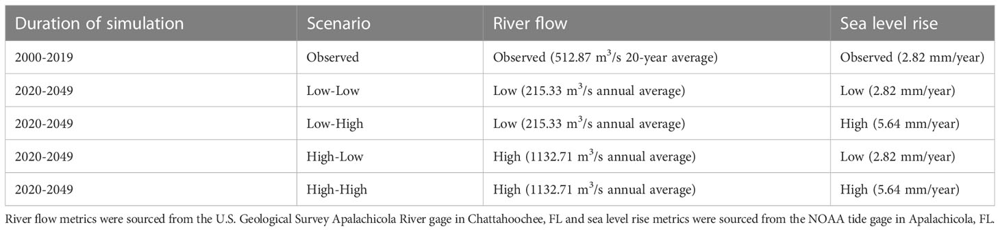
Table 2 River flow and sea level rise conditions observed from 2000 through 2019 used to hindcast the hydrodynamic model (Observed scenario) and future scenario parameters used to simulate different combinations of river flow and sea level rise in Apalachicola Bay from 2020 through 2049.

FIGURE 2

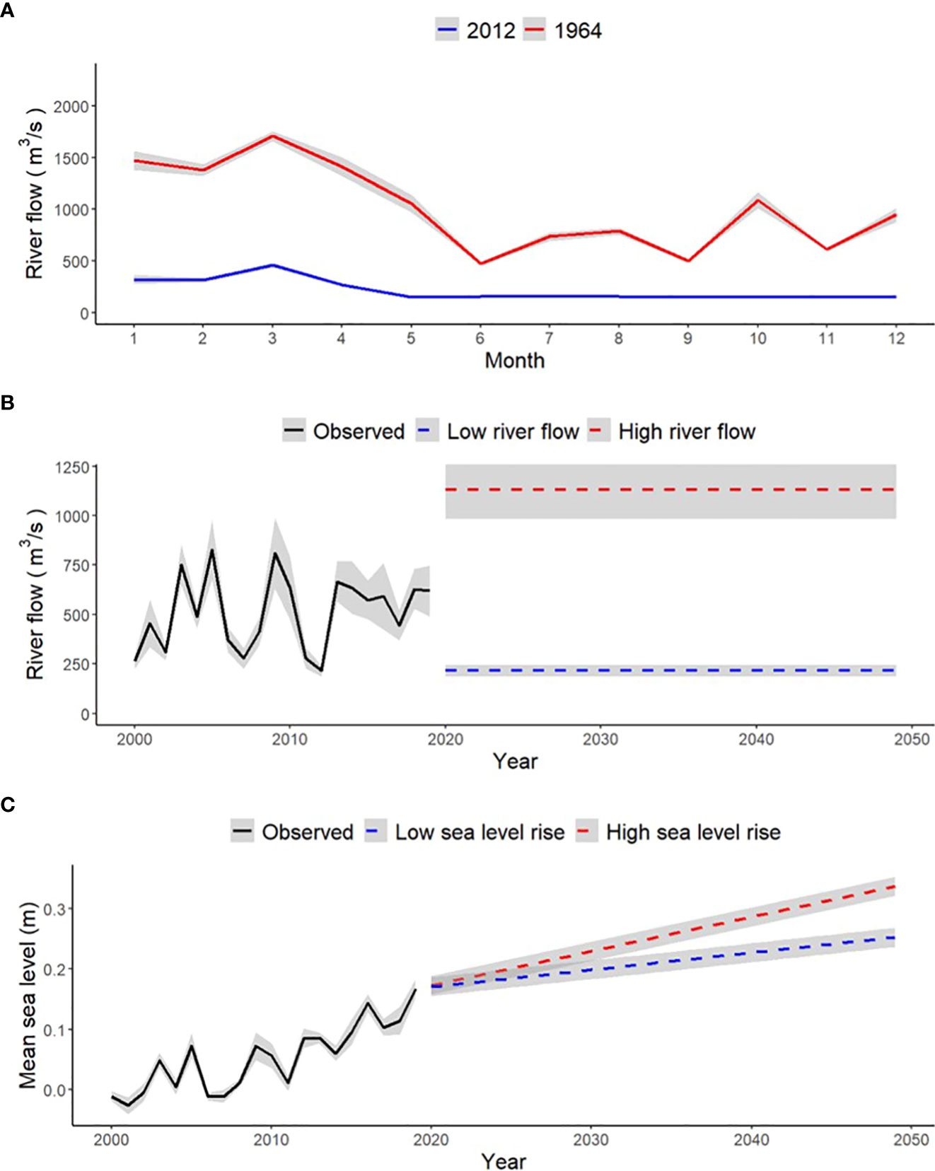
Figure 2 (A) Monthly average Apalachicola River flow (with a 95% confidence interval) at historically low levels in 2012 and historically high levels in 1964. (B) Observed annual average Apalachicola River flow (with a 95% confidence interval) from 2000 to 2019 with projected annual average river flow (with a 95% confidence interval) during future scenarios of low and high river flow conditions from 2020 to 2049. The monthly river flow variations in plot A were used to simulate the future scenarios of low and high river flow through the hydrodynamic model by repeating the same monthly flow patterns across each year of the future scenarios. (C) Observed annual average sea level (with a 95% confidence interval) from 2000 to 2019 and projected annual average sea level (with a 95% confidence interval) under low and high sea level rise conditions from 2020 until 2050 simulated through the hydrodynamic model for Apalachicola Bay.

Spatial temporal food web model simulations using Ecospace

The Ecospace module of EwE was used to represent the combined temporal and spatial dynamics within the Apalachicola Bay system. Ecospace depicts spatial-temporal dynamics in the form of a georeferenced base map where the differential equations utilized in Ecosim (Eqs. 3 and 4) are applied across each grid cell of the base map (Walters et al., 1999; Christensen and Walters, 2004). The domain of the Apalachicola Bay Ecospace model encompasses the eight sampling sites visited as part of ANERR’s trawl monitoring surveys (Figure 1) and consists of a network of 250 m² resolution grid cells. Cells with water within the model domain are considered active cells that can receive environmental input and be occupied by species and fishing groups. All other cells are considered inactive. ASCII grid files output from the hydrodynamic model representing depth, water temperature and salinity served as the foundation for the Ecospace model. Additional ASCII grid files were included to delineate oyster reef and seagrass habitat areas (sourced from geodata.myfwc.com) and represent primary production spatial dynamics (based on chlorophyll a concentrations measured by the SWMP nutrient monitoring sites, Figure 1).

A series of ASCII grid files of primary production, salinity and temperature at monthly time steps were used to drive changes over space and time in Ecospace. The series of monthly grid files spanned all 20 years of the observed time period (2000 to 2019). Measures of salinity and temperature across the model domain drove changes in species distributions according to each species’ environmental tolerances. The species response curves used to represent environmental tolerances in Ecosim were transferred to Ecospace. The habitat capacity model (Christensen et al., 2014; described earlier in Model calibration in Ecosim) computes the suitability of each spatial grid cell for species inhabitance based on habitat and environmental conditions. Oysters and seagrass were the only species groups in the model restricted by habitat type (confined to oyster reefs and seagrass habitat respectively). All species groups with activated response curves directly responded to changes in water temperature and salinity. At each monthly time step, Ecospace displayed map images of biomass concentrations for each species group in the model in response to the environmental input. The Ecospace food web model simulations were first run over the observed period (2000-2019, Observed scenario in Table 2) before simulating future conditions from 2020 through 2049.

To simulate the future scenarios of varying river flow and sea level rise conditions (Table 2), ASCII grid files of environmental parameters at monthly time steps representing the years 2020 through 2049 were appended to the series of files spanning the initial period. Each scenario was run separately in Ecospace using the scenario outputs of salinity and temperature from the Delft3D model. Fishing effort was kept constant across the future scenarios by using the mean effort from 2000 to 2019, except for the oyster fishery, where a moratorium was instituted from 2020 through 2025 (Elliott, 2020). Primary production levels were kept constant across all future scenarios by repeating the observed patterns from the initial period. The resulting temporal and spatial changes in species biomasses in response to the environmental drivers were output as monthly ASCII maps of biomass for each year of the simulation.

Stakeholder survey

A survey of Apalachicola Bay stakeholders was developed to explore local ecological knowledge (LEK) of how river flow and sea level rise in the Apalachicola Bay area contribute to species and environmental changes. For the context of this study, a stakeholder was defined as anyone who lives in the Apalachicola Bay system or whose work pertains to the system. Survey questions were designed in collaboration with ANERR staff and scientists to determine stakeholders’ relationship to the Apalachicola Bay estuary (Appendix J). Relationships were categorized by each stakeholder’s personal impression of 1) which resident fish and invertebrate species they considered to be commercially or recreationally important, 2) their knowledge of how changes in river flow and sea level may or may not impact important fishery species, and 3) the perceived impact of those changes to stakeholders themselves.

The survey was programmed using ESRI ArcGIS Survey123 software and participants were recruited by emailing known contacts of ANERR, in-person engagement of the local community, and sharing the survey on social media. Over a seven-month period, the survey garnered a total of 37 responses from participants who were asked to identify themselves as either a scientific researcher, commercial fisher, seafood worker, recreational fisher, charter boat captain, government employee or representative, non-profit organization representative or a local community member (or some combination of these roles; Appendix K). Survey results were used to determine commercially and recreationally important species to direct the focus of the food web model analysis and assess the perceived impacts of climate change on environmental conditions, Apalachicola Bay species and the stakeholders themselves.

Analysis

Coupled hydrodynamic and food web model results were used to assess the impacts of changes in river flow and sea level rise on Apalachicola Bay environmental conditions (i.e., salinity and temperature), individual species’ biomass and distribution, as well as total food web biomass and upper trophic level diversity as represented by Kempton’s Q index. To better visualize spatial changes in total biomass across Apalachicola Bay, oyster and seagrass biomasses were excluded from the annual average total biomass maps as these species were stationary in the spatial-temporal model framework and had high biomass values that obscured any spatial changes in the biomasses of mobile species in the model. As calculated by EwE, Kempton’s Q index is a measure of biomass diversity of organisms with trophic level ≥ 3 where the Q value is proportional to the inverse slope of the species-abundance curve (Ainsworth and Pitcher, 2006). Kempton’s Q index can be interpreted as a proxy for ecosystem biodiversity, with higher Q values corresponding to greater biodiversity (Ainsworth and Pitcher, 2006). Out of the many ecological indicators calculated by Ecospace, total biomass and Kempton’s Q index were chosen for focus by this study to address broader food web dynamics because they were representative of the entire food web, while many of the other indicators are specific to different sub-groups (Coll and Steenbeek, 2017). All model results compared the percent change in annual means of each variable (salinity, temperature, biomass, etc.) between 2019 and 2049 for each of the future scenarios of river flow and sea level rise, along with the spatial distributions of each given variable over time. Since the hydrodynamic and food web model outputs lack statistically independent samples, statistically significant differences in environmental or species variables were unable to be assessed. Rather, the model results serve as a visualization of the range of potential impacts changes in river and sea level rise may have on the abiotic and biotic characteristics of Apalachicola Bay.

Survey results were used to assess stakeholder perceptions about how future freshwater reduction and sea level rise may impact Apalachicola Bay environmental conditions, commercially and recreationally important fisheries species, and the human community (Franklin County economy, stakeholder profession, and personal interaction with the estuary) of the Apalachicola Bay system. Stakeholder survey questions were first used to assess stakeholder perceptions about how a future reduction in river flow or increase in sea level would affect water temperature and salinity in Apalachicola Bay. Survey results were also used to determine which Apalachicola Bay species were regarded as commercially and recreationally important. Survey participants were given a pre-defined list of species and asked to select which species they considered to be the most commercially or recreationally important. The pre-defined list was based on fishery species that were well represented in the ANERR trawl survey data. Though oysters are known as a highly valued commercial fishery species in Apalachicola Bay, they were excluded from the survey list because the intent of the study was to give greater focus to nekton species. Survey participants were made aware that oysters were excluded from the list. Participants had the option to write in a different answer if a species they considered commercially or recreationally important was not included on the list. Further analysis of the stakeholder survey, as well as analysis of the food web model results, focused on the top selections of commercially and recreationally important species reported by the survey (commercial shrimp and flounders). After survey participants selected a commercially or recreationally important species, they were asked a subset of questions pertaining to how they thought a future reduction in river flow or increase in sea level would impact the selected species population in Apalachicola Bay. Effects of future changes in river flow and sea level rise on the human community of Apalachicola Bay were assessed using survey responses on impacts to the Franklin County economy (where Apalachicola Bay resides), each stakeholder’s profession and each stakeholder’s personal interaction with Apalachicola Bay. Personal interaction with Apalachicola Bay could include activities such as fishing, birding, hiking, boating or any engagement with the ecosystem outside of the participant’s profession. The survey results served as a point of comparison to evaluate the agreement of the model simulation results with stakeholder perceptions of environmental and species population changes. This combined approach provides a novel method to understand how changes in an estuarine food web can potentially impact the human communities that rely on these systems.

Given the complexity of the study, the results are organized around three general topics: 1) Impacts to environmental conditions (water temperature and salinity), 2) Impacts to species of commercial and recreational fishing importance and 3) Impacts to the broader food web (total biomass and upper trophic level diversity) and human community (Franklin County economy, stakeholder profession, and personal interaction with the estuary) of Apalachicola Bay.

Results

Environmental conditions

Model results

Predicted mean temperature for year 2049 increased across all scenarios relative to the observed mean for 2019 (Figure 3A). The greatest predicted increases in annual mean temperature occurred during low river flow scenarios (+13%; Figure 3A). Mean salinity for 2049 increased during the low river flow scenarios (+11% in the Low-Low scenario and +13% in the Low-High scenario; Figure 3A) and decreased during the high river flow scenarios (-61% in the High-Low scenario and -59% in the High-High scenario; Figure 3A). Within the low or high river flow scenarios, there were little differences in 2049 mean temperature and salinity compared across different sea level rise conditions (Figures 3A).

FIGURE 3

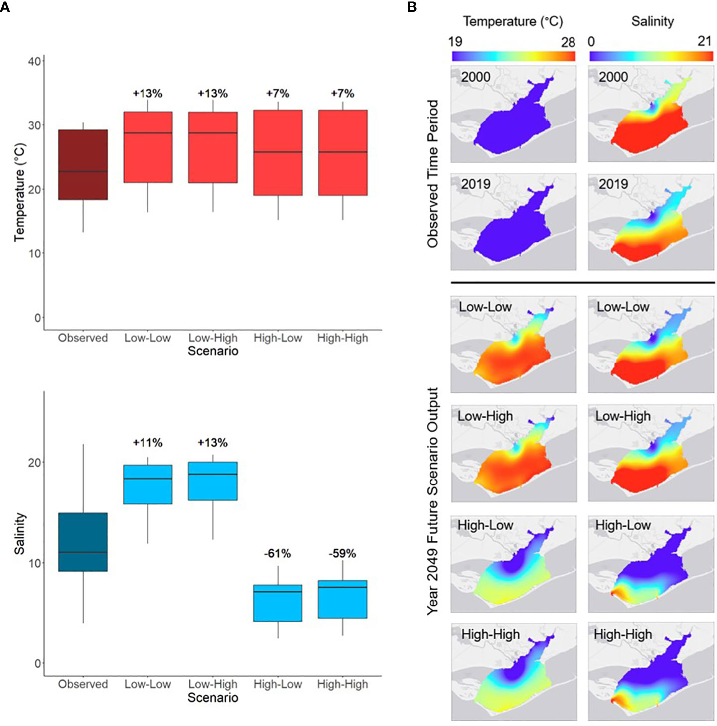
Figure 3 (A) The annual range of Apalachicola Bay water temperature (° C) and salinity averaged over the entire study area between year 2019 (Observed) and year 2049 of each of the future scenarios. Percent changes indicate the difference between the 2049 annual mean of each scenario and the 2019 annual mean. (B) Spatial variation in annual average water temperature (° C) and salinity in Apalachicola Bay during the beginning (2000) and end (2019) of the observed time period and year 2049 of each of the future scenarios. Scenario names define the river flow conditions first, followed by sea level rise conditions (e.g., Low-High indicates low river flow and high sea level rise; scenario parameters defined in Table 2).

Apalachicola Bay water temperature and salinity spatially varied over time. Annual average water temperature showed greater spatial variation in 2049 compared to 2000 and 2019 (Figure 3B). Across all future scenarios, annual average temperatures were highest in the southern region of Apalachicola Bay, with the warmest temperatures present during low river flow scenarios (Figure 3B). During the observed years (2000 and 2019), annual average salinity was higher in the southern regions of the bay, while the northern region (closest to freshwater inflow) was less saline (Figure 3B). A similar pattern occurred in 2049 for both the low river flow scenarios. Low salinity levels covered much of the southern region of the bay during high river flow scenarios (Figure 3B).

Survey results

Most survey participants (~43%) thought a future reduction in river flow would increase water temperature (Figure 4A). Survey results also indicated that most participants (~32%) assumed an increase in sea level would have little to no effect on water temperature, though a large proportion (~30%) said water temperature would increase (Figure 4B). Both a future reduction in river flow and increase in sea level were largely thought to result in an increase in salinity (~89% in Figure 4A, ~76% in Figure 4B).

FIGURE 4

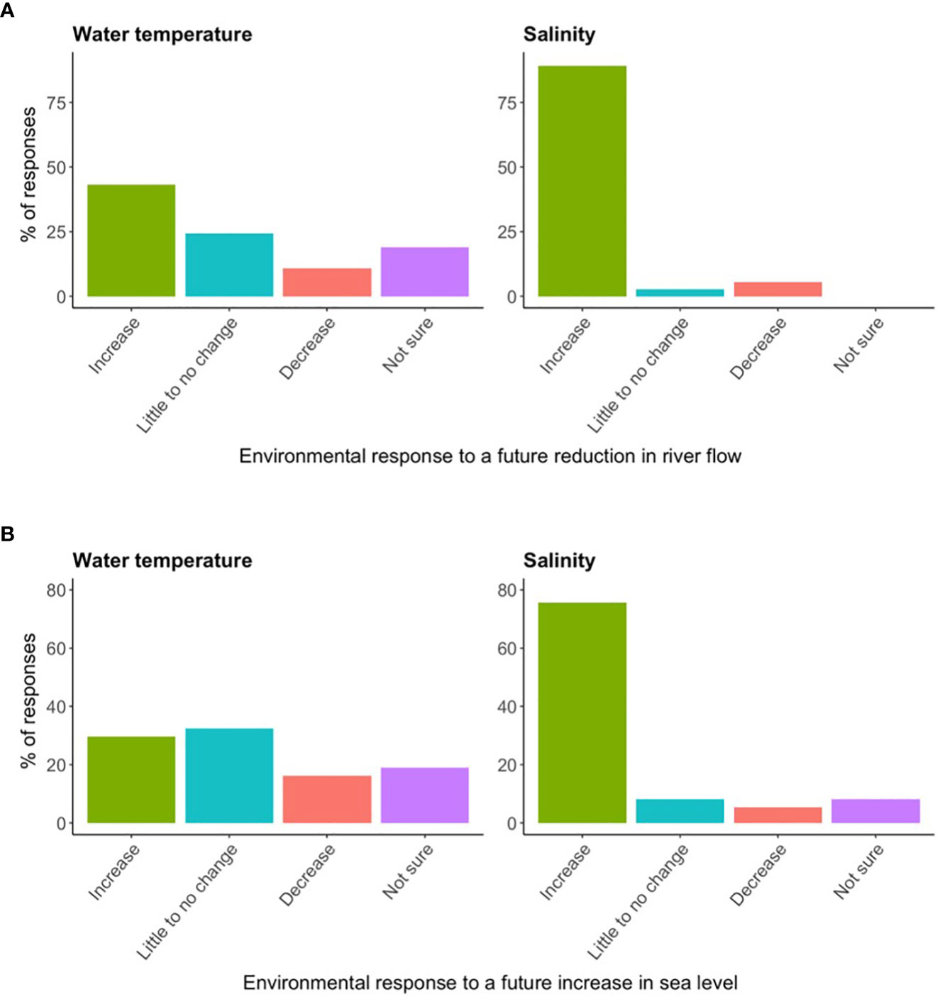
Figure 4 The percentage of survey responses indicating stakeholder perceptions regarding how potential future reductions in river flow and sea level rise would affect Apalachicola Bay water temperature and salinity (n = 37). (A) Pertains to river flow and (B) pertains to sea level rise.

Impacts to important commercial and recreational fishery species

Model results

Specific focal species were chosen based on those identified as the most commercially or recreationally important in the stakeholder survey (see Survey results below), which consisted of white shrimp and Gulf flounder (Appendix L). Since white shrimp was a multi-stanza group in the food web model, analysis focused on both the juvenile and adult populations of the species. Model outputs predicted that both juvenile and adult white shrimp biomass would increase between 2019 and 2049 for the low river flow scenarios and decrease during the high river flow scenarios (Figure 5A). Gulf Flounder mean biomass was predicted to decrease between 2019 and 2049 for all scenarios. The largest predicted percent decrease occurred during the High-Low scenario (-78%, Figure 5A).

FIGURE 5

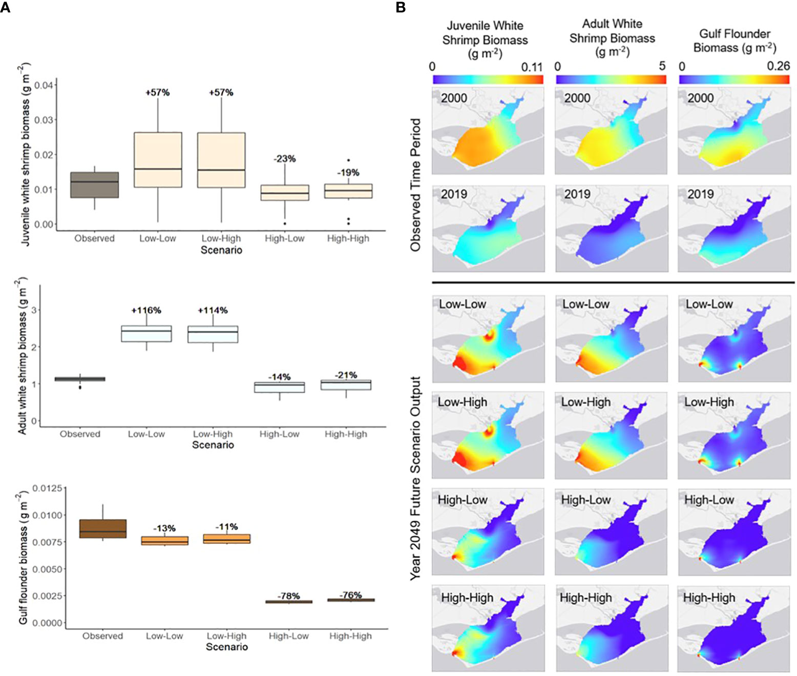
Figure 5 (A) The annual range of spatially-averaged biomass (g m^-2) for white shrimp (juvenile and adult) and Gulf flounder in Apalachicola Bay between year 2019 (Observed) and year 2049 of each of the future scenarios. Percent changes indicate the difference between the 2049 annual mean species biomass of each scenario and the 2019 annual mean. (B) Spatial variation in annual average biomass (g m^-2) of white shrimp (juvenile and adult) and Gulf flounder in Apalachicola Bay during the beginning (2000) and end (2019) of the observed time period and year 2049 of each of the future scenarios. Scenario names define the river flow conditions first, followed by sea level rise conditions (e.g., Low-High indicates low river flow and high sea level rise; scenario parameters defined in Table 2).

Model outputs showed that spatial distributions of white shrimp and Gulf flounder changed across the observed time period and future scenarios. Species distribution patterns were more similar between future scenarios defined by the same river flow conditions rather than those defined by the same sea level rise conditions (e.g., there was a greater resemblance between the Low-Low and Low-High scenarios than between the Low-Low and High-Low scenarios; Figure 5B). Biomasses of both juvenile and adult white shrimp were higher in the southern (particularly southwestern) portion of Apalachicola Bay across all years and scenarios (Figure 5B). In the high river flow scenarios, white shrimp biomass, for both juveniles and adults, was low across the northern, middle, and southeastern regions of the bay (Figure 5B). Gulf flounder biomass was generally higher in the southern region of Apalachicola Bay (Figure 5B). For all future scenarios, Gulf flounder biomass was low across much of the bay, except for near two small passes connecting to the Gulf of Mexico (Figure 5B).

Survey results

Most survey participants (~54%) selected commercial shrimp as the most commercially important species (outside of oysters) in Apalachicola Bay (Appendix L). For recreationally important species, most survey participants selected flounders (~22%; Appendix L). Survey responses indicated that most participants who selected commercial shrimp and flounders thought a future reduction in river flow would result in a decrease in the populations of these species (Figure 6A). An anticipated increase in sea level was expected to have more variable impacts on species. For commercial shrimp, most participants (~40%) thought the population would decrease in response to an increase in sea level, though a large proportion (~35%) were not sure of the possible effect (Figure 6B). For flounders, the majority of participants thought the population would decrease (~50%; Figure 6B).

FIGURE 6

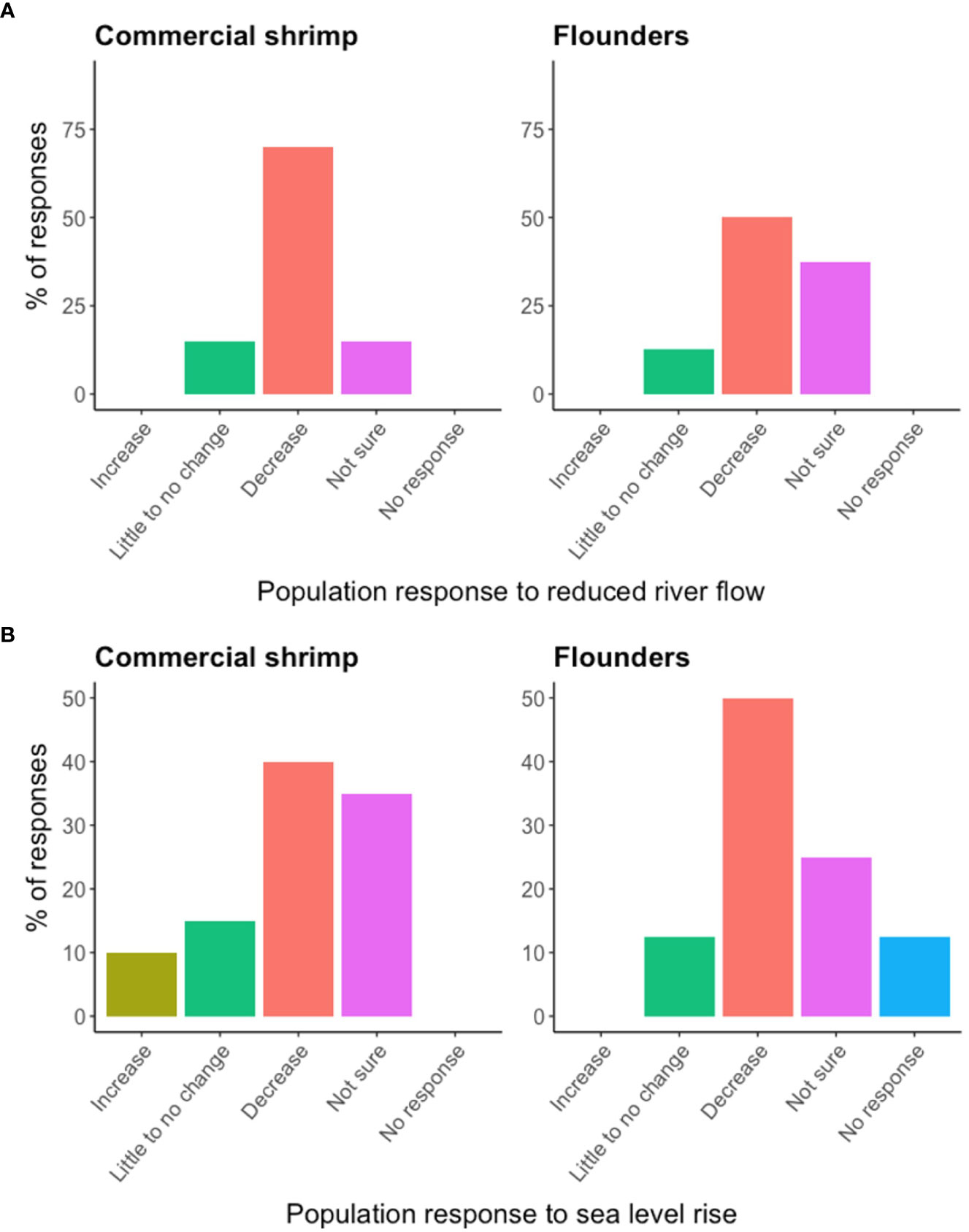
Figure 6 The percentage of survey responses indicating the anticipated impact of a future reduction in river flow or increase in sea level on populations of commercially important commercial shrimp (n = 20) and recreationally important flounder (n = 8) populations in Apalachicola Bay. (A) Pertains to river flow and (B) pertains to sea level rise.

Impacts to the broader food web and human community

Model results

Mean total biomass of the entire food web between year 2019 and year 2049 was predicted to increase by similar percentages across all scenarios (Figure 7A). Mean Kempton’s Q index decreased between 2019 and 2049 for all scenarios, with the largest percent decrease occurring during the High-Low and High-High scenarios (-17%; Figure 7A). Total biomass and Kempton’s Q index also varied spatially across the observed period and future scenarios. Annual average total biomass exhibited the greatest spatial variation in 2000 (Figure 7B). In 2019, annual average total biomass was highest in the southwestern region of Apalachicola Bay and highest in the bay’s northern region in 2049 (Figure 7B). Annual average values of Kempton’s Q index had greater spatial variation in 2000 and 2019, while the spatial patterns became more uniform across the future scenarios (Figure 7B). Kempton’s Q index values were generally higher in the southern region of Apalachicola Bay for all future scenarios (Figure 7B).

FIGURE 7

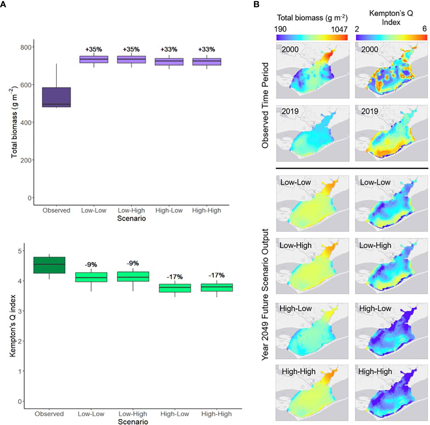
Figure 7 (A) The annual range of spatially-averaged total biomass (g m^-2) and Kempton’s Q index in Apalachicola Bay between year 2019 (Observed) and year 2049 of each of the future scenarios. Percent changes indicate the difference between the 2049 annual mean of each scenario and the 2019 annual mean. (B) Spatial variation in total average biomass (g m^-2) of spatially mobile species and Kempton’s Q index in Apalachicola Bay during the beginning (2000) and end (2019) of the observed time period and year 2049 of each of the future scenarios. Total biomass represents the biomass of all species in the food web model except the stationary oyster and seagrass groups. Scenario names define the river flow conditions first, followed by sea level rise conditions (e.g., Low-High indicates low river flow and high sea level rise; scenario parameters defined in Table 2).

Survey results

Most survey responses indicated the perception that both a future reduction in river flow (~84%, Figure 8A) and increase in sea level (~84%, Figure 8B) would have a negative impact on the Franklin County economy. Most survey participants also thought that these future environmental changes would have little to no impact on their professions (~65% Figures 8A, ~54% Figure 8B). In terms of participants’ personal interactions with Apalachicola Bay, the majority thought a future reduction in river flow would have a negative impact (~49%, Figure 8A) and a future increase in sea level would have little to no impact (~51%, Figure 8B). It should be noted that the results of the stakeholder survey are merely reflective of the demographic of survey participants. There was a lack of participants with fishing-related professions, so the reported survey results are not necessarily representative of all stakeholders for the Apalachicola Bay system.

FIGURE 8

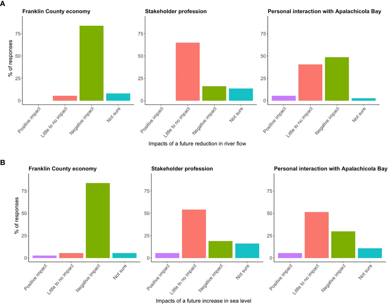
Figure 8 The percentage of survey responses indicating stakeholder perceptions regarding how potential future reductions in river flow and sea level rise would impact the Franklin County economy, the stakeholder’s profession, and the stakeholder’s personal interaction with Apalachicola Bay (n = 37). (A) Pertains to river flow and (B) pertains to sea level rise.

Discussion

Estuarine systems across the globe are increasingly subject to the combined influence of climate change and human-induced stressors (Trenberth, 2011; Hoegh-Guldberg et al., 2014). Resulting shifts in environmental conditions can alter estuarine community structure at all levels of the food web (Greenwood et al., 2007; Gillanders et al., 2011; Guenther and Macdonald, 2012; James et al., 2013; Little et al., 2017; Garwood et al., 2023). The Apalachicola Bay estuary is one such example where climate- and anthropogenically-driven changes in river inflow and sea level impact the abundances and distributions of species in the system, many of which are considered commercially or recreationally important (Livingston, 1982; Livingston et al., 1997; Livingston et al., 2000; Huang et al., 2015; Kimbro et al., 2017; Garwood et al., 2023). This study used a coupled hydrodynamic and food web model, along with a survey of local stakeholders, to determine the potential impacts of 30-year future scenarios of low and high river flow and sea level rise on the Apalachicola Bay food web. Analysis of the results focused on predicted impacts to environmental conditions and populations of commercially and recreationally important species in Apalachicola Bay, and impacts from a broader food web perspective. Predicted changes in these biotic and abiotic factors were largely different between scenarios of low and high river flow, while model simulations suggested there would be little difference between the low and high sea level rise. This outcome indicates that Apalachicola River flow is the primary driver for the biotic and abiotic factors in Apalachicola Bay. The hydrodynamic and food web model simulations provided a point of comparison with stakeholder concerns regarding anticipated future changes in abiotic and biotic characteristics of the estuary. By synthesizing long-term monitoring data with LEK, this study creates a localized portrayal of potential future impacts of climate change and human-induced stressors on both the estuarine food web and human community, an approach that may be informative to other estuarine systems.

Environmental conditions

Different future river flow and sea level rise conditions are expected to result in an increase in Apalachicola Bay water temperature; however, those same conditions could cause an increase or decrease in bay salinity. Most survey respondents thought a reduction in Apalachicola River flow would increase the bay’s water temperature and an increase in sea level would result in either little to no change or an increase in temperature. The modeled output of the environmental conditions generally agreed with the results of the survey. The continual increase in water temperature across future scenarios aligns with previous studies that suggest global estuarine water temperatures may increase with air temperature as a result of climate change (Scavia et al., 2002; Najjar et al., 2010; Cloern et al., 2011; Altieri and Gedan, 2015). Future sea surface temperatures in the Gulf of Mexico are expected to increase (Muhling et al., 2011), therefore, the predicted sea level rise in the region would bring warmer sea water into Apalachicola Bay. The water temperature of river inflow may also increase as a result of reduced flow volume upstream (Mosley, 2015).

While predicted water temperature increased across all future scenarios, there were distinct differences in salinities between scenarios of low and high river flow. Most stakeholder survey participants thought a reduction in river flow and increase in sea level rise would increase Apalachicola Bay salinity, and the hydrodynamic model results largely supported this perception. Low and high sea level rise conditions coincided with an increase in salinity when coupled with low river flow, but not when coupled with high river flow. Based on the sea level rise scenarios utilized in this study, relative mean sea level estimates in 2050 (0.14 m under low sea level rise, 0.28 m under high sea level rise, relative to a baseline of 2000) most closely resembled those of the low and intermediate global sea level rise scenarios describe in Sweet et al., 2022, meaning they are somewhat conservative compared to more drastic global projections. However, other studies have further corroborated the dominant influence of Apalachicola River flow on estuarine salinity (Sun and Koch, 2001; Morey and Dukhovskoy, 2012), even when paired with global sea level rise projections (Huang et al., 2015). The use of the hydrodynamic model to simulate changes in both river flow and sea level rise provides insight on the coupled effects of these stressors and more nuanced potential outcomes for the system.

Fisheries species

The anticipated impacts of changes in river flow and sea level rise on commercially important white shrimp differed between the food web model and stakeholder survey results. The increase in biomass under low river flow conditions and decrease with high river flow conditions exhibited by the food web model can largely be attributed to a broad salinity tolerance (approximate optimum range of 5 – 35 ppt) and preference for warmer temperatures (~ 25-30° C) defined by the environmental response curves for white shrimp (Appendices D, E). An increase in white shrimp predator biomass, such as red drum (Appendix A; Scharf and Schlicht, 2000), likely contributed to the decrease in white shrimp biomass during high river flow scenarios as well. The modeled response of white shrimp did align with results of previous studies that associate greater juvenile white shrimp abundance with higher salinities and temperatures (Diop et al., 2007; Gómez-Ponce et al., 2021; Garwood et al., 2023). White shrimp catch per unit effort has also been negatively correlated with river discharge across the Gulf of Mexico and in South Carolina (Millberry, 2013; Fowler et al., 2018). In contrast to the food web model results, survey responses suggested a decrease in the Apalachicola Bay commercial shrimp population in response to reduced river flow and increased sea level. This perception may be based on historical trends in shrimp fishery landings, which have previously dropped by 90% after drought events in the Apalachicola Bay system (Livingston, 2008), though these landings generally consist of catch from across the northern Gulf of Mexico. A wide range of factors such as altered habitat conditions, enhanced predation, competition and disease likely played a role in the historical shrimp population decline (Livingston, 2008). While the food web model incorporated species environmental tolerances and trophic dynamics, other factors such as changes in habitat, disease prevalence and influxes of new species were not represented. The assessment of these additional factors may provide further insight regarding the differences in modeled trends versus those anticipated by stakeholders.

Gulf flounder, a species of recreational fishing interest, was predicted to decrease in abundance across both the model and stakeholder survey results. In the food web model, Gulf flounder exhibited a preference for high salinities (25-30 ppt, Appendix D) and temperatures (20-30° C, Appendix E). Gulf flounder prey (zoobenthos, and macro- and microzooplankton; Appendix A) biomasses were predicted to increase across all scenarios (Appendix M), so it appears the environmental tolerances of Gulf flounder were more indicative of a decline in biomass than prey availability. Recent studies on Gulf flounder population dynamics are limited, but historically, juvenile Gulf flounder abundances have been shown to be highest at the mouths of Florida estuaries where salinities tend to be highest (Gilbert, 1986). Our model outputs suggested a similar pattern for all future scenarios. Concentrations of Gulf flounder biomass were predicted to be highest near the southern passes of Apalachicola Bay, which tend to be higher in salinity because of the close proximity to the Gulf of Mexico. An earlier habitat suitability index for Gulf flounder determined their optimal salinity and temperature conditions to be 15-40 ppt and 15-35° C (Enge and Mulholland, 1985). Due to their high salinity preference, Gulf flounder are highly susceptible to change via altered salinity structure in Gulf of Mexico estuaries (Christensen et al., 1997); therefore salinity and sea level may function as strong predictors of population variability over time (Fujiwara et al., 2016). Results from the stakeholder survey indicated an anticipated decrease in flounder populations due to reduced river flow and increased sea level rise. The food web model results aligned with this prediction because the increase in salinity across the low river flow scenarios still fell short of the optimal range for Gulf flounder, resulting in a decrease in biomass across both future low and high river flow and sea level rise conditions in Apalachicola Bay.

Changes in river flow and sea level rise in Apalachicola Bay are likely to have variable impacts on the commercial and recreational fisheries for the region. Oysters were historically known as the most important commercial fishery in Apalachicola Bay and experienced a population decline due to low river inflow during times of drought, particularly in 2007 and 2012 (Livingston, 2008; Havens et al., 2013). Drought periods corresponded with a decline in landings of other commercially important species such as white shrimp and blue crab in Apalachicola Bay as well (Livingston, 2008), though catch from these landings may be sourced from across the northern Gulf of Mexico. Results of this study and others indicate that low river flow conditions (in combination with either low or high sea level rise) have the potential to positively impact the commercial white shrimp fisheries through increases in the biomass of the species (Garwood et al., 2023). With a decrease in white shrimp biomass observed during the high river flow scenarios in this study, these conditions may be less ideal for commercial fishery landings. White shrimp is one of the top ten commercially valued species in Franklin County, FL (Commercial Fisheries Landings Summaries Database, 1986) so changes in the population will have implications for the local economy. However, it must be noted that the model results are only a representation of potential outcomes, and changes in species biomasses are primarily driven by environmental tolerances and predation/prey availability in the current model version. Incorporating additional influences on species biomasses, such as habitat changes and disease prevalence, may provide additional insight on species responses to changes in river flow and sea level rise. Recreational fishing occurs throughout Apalachicola Bay and will be impacted by changes in the populations of recreationally valued species, such as Gulf flounder. With the potential for both increased future drought and precipitation events in the Apalachicola Bay watershed, the model simulation results of this study indicate mixed effects on fisheries species within the estuary.

Broader Apalachicola Bay food web and human community

The broader Apalachicola Bay food web, specifically total biomass and upper trophic level diversity will be impacted by future changes in river flow and sea level rise. The total biomass of the food web increased in all simulated future scenarios, while upper trophic level diversity (measured by Kempton’s Q index) decreased. Historically, drought and reduced river flow have led to a decline in fish species richness and trophic diversity in Apalachicola Bay (Livingston, 1997), but there has been no report of high river flow having a similar effect. Other studies of estuaries around the world have reported similar trends of increased food web biomass and decreased species diversity due to changes in the estuarine salinity regime (Flores-Verdugo et al., 1990; Barletta et al., 2003; Whitfield, 2005; Fujii and Raffaelli, 2008). The increase in total biomass and decrease in diversity across scenarios in this study may be due to an increase in abundance of individual species that prefer different salinity regimes and a decrease in abundance of species unable to tolerate the new environmental conditions. However, the results of this study are only representative of the limited species groups represented in the food web model and are not able to account for increased abundance of new species that were not present in the original monitoring data that might occur as a result of the future scenarios.

Future changes in river flow and sea level rise would affect the human community of Apalachicola Bay. Results of the stakeholder survey indicated an anticipated negative impact to the Franklin County economy due to reduced river flow and increasing sea level rise. Much of the Franklin County economy is based on commercial and recreational fishing (Edmiston, 2008) and past drought events have resulted in reduced landings of several fishery species, such as oysters, shrimp, and blue crab, due to a reduction in river inflow to Apalachicola Bay (Livingston, 2008; Havens et al., 2013). Declines in fishery species populations can have lasting impacts, as has been the case with the Apalachicola Bay oyster fishery, which has failed to recover since its collapse in 2012 and was put under a five-year moratorium in 2020 (Hallerman, 2021). Simulation results of this study indicate that reduced river flow in combination with sea level rise may not always have such negative impacts, as the biomass of commercially important white shrimp was predicted to increase during scenarios of low river flow. Many stakeholders also anticipated a reduction in river flow negatively impacting their personal interaction with Apalachicola Bay. Some of the most common recreational activities in the Apalachicola Bay region that might constitute “personal interaction” are fishing, camping, and hiking (Shrestha et al., 2007). While this study is not able to assess the terrestrial impacts of changes in river flow and sea level rise, the food web model results did indicate decreases in biomass of recreationally important Gulf flounder that stakeholders might value in their personal interaction with Apalachicola Bay. A more optimistic result of the stakeholder survey was the largely anticipated little to no impact of a reduction in river flow and increase in sea level on the professions of survey participants. However, this is limited to the demographic of survey participants, many of which held government or scientific researcher professions that are less likely to be directly affected by environmental changes. Had a greater proportion of recreational or commercial fishers participated in the survey, the answers regarding river flow and sea level rise impacts on stakeholder profession may have changed.

Future directions

There are several future directions that would help expand upon the study at hand. Firstly, the model results presented in this study reflect annual average measures of environmental conditions, species biomasses and Kempton’s Q index, and are not representative of seasonal changes that may occur in these variables. Analysis of seasonal trends would be useful for better understanding species recruitment dynamics in the estuary. The environmental conditions presented in this study were limited to salinity and temperature, but Apalachicola River is also a major nutrient source to the bay (Mortazavi et al., 2000), so changes in river flow would affect nutrient loads within the estuary. Higher nutrient loads and subsequently primary production have been associated with increased river inflow to Apalachicola Bay (Huang, 2010). Eutrophication is generally not an issue of concern for Apalachicola Bay due to its relatively short residence time (Huang and Spaulding, 2002; Livingston, 2008). This study was unable to incorporate changes in nutrient loads in response to river flow and sea level rise, so further simulations of these changes and their impact on the food web would add greater depth to the study results. The food web model simulations were also limited by the model domain, which did not encompass the more saline channels (St. Vincent Sound and St. George Sound) that connect the western and eastern regions of Apalachicola Bay to the Gulf of Mexico. Thus, the results were unable to portray potential shifts in species distributions to these areas in response to environmental changes. While the focus of this study was on the Apalachicola Bay region where long-term monitoring data were available, the incorporation of species data from St. Vincent and St. George Sounds would provide a more complete picture of changes in species abundance and distributions in response to river flow and sea level rise. Ecospace is also limited by the inability to calibrate spatial data. While species biomasses and environmental variables were able to be calibrated over time using Ecosim, the same functionality does not yet exist for Ecospace. Though the calibrated Ecosim model serves as the foundation for species dynamics in Ecospace, further study mapping observed species distributions over time would be valuable to compare with the food web model results to assess the goodness of fit of the simulated spatial dynamics of the food web.

While the future scenarios described were particular to Apalachicola Bay, this study exemplifies the use of local monitoring data to assess system-specific stressors in an estuarine ecosystem. Climate change and anthropogenic disturbances will have variable future impacts on estuaries across the globe. Estuaries in Mediterranean-type climates are likely to become warmer and drier due to climate change, while those in more northern climates may experience increased precipitation due to greater frequency and intensity of storm events (Najjar et al., 2010; Gillanders et al., 2011; Hallett et al., 2018). Our study highlighted freshwater inflow as a major influence on the abiotic and biotic characteristics of Apalachicola Bay, but in other estuarine systems sea level rise may play a more dominant role (Yang et al., 2015; Robins et al., 2016; Vargas et al., 2017). With a high degree of variability in climate change and human impacts on estuarine systems, it is difficult to generalize future predicted changes across regions (Robins et al., 2016; Biguino et al., 2023). Thus, it is critical to incorporate localized, long-term monitoring data into the assessment of climate change impacts and projections for estuarine systems and promote the development of mitigation plans (Biguino et al., 2023). This study highlights the use of such abiotic and biotic data to develop predictive models and scenarios and evaluate impacts to environmental conditions, individual species, and the broader estuarine food web at a realistic, regional scale.

In addition to the scientific knowledge conveyed through monitoring data and ecosystem models, it is also important to consider LEK in the assessment of localized climate and human impacts on estuarine systems (Sánchez-Jiménez et al., 2019). The examination of both food web dynamics and human dimensions in this study serves as an example of the comparison of food web modeling analysis and stakeholder perceptions to better understand changes occurring in the system. In some cases, the model and stakeholder survey results were complementary (environmental conditions, Gulf flounder), while in others there were differences between the two (white shrimp). Instances where discrepancies were present between model results and stakeholder perceptions provide areas of further investigation into the reasoning behind these differences. Sánchez-Jiménez et al. (2019) suggests that discrepancies between LEK and scientific knowledge may indicate sources of management problems to be addressed with further study. Considering both scientific knowledge and LEK is important for developing management practices that are accepted by the whole community (Mackinson et al., 2011). The comparison of stakeholder knowledge and perceptions with modeled simulations is an approach that can be adapted to assess stressors specific to other estuarine systems as well. Utilizing multiple knowledge sources provides a more nuanced understanding of the system (Sánchez-Jiménez et al., 2019). More ecosystem modeling studies around the world have begun to involve stakeholders in the model development process and the framing of research questions (Fulton et al., 2015; Koenigstein et al., 2016; Miller et al., 2017; Bélisle et al., 2018). This co-production of knowledge between researchers and local stakeholders is important for providing actionable science that can be of use to natural resource managers (Beier et al., 2017).

Conclusions

The results of this study indicated variable impacts of future changes in river flow and sea level rise on environmental conditions, commercially and recreationally important fishery species and local stakeholders of Apalachicola Bay. Water temperature is likely to continually increase while Apalachicola Bay salinity will largely be influenced by river inflow. Changes in the estuarine salinity regime may be of benefit or detriment to commercially or recreationally important fishery species, such as white shrimp and Gulf flounder. Modeled simulations indicated a transition to greater total food web biomass and less upper trophic level diversity in response to future environmental changes. Stakeholders anticipate negative impacts of reduced river inflow on the Franklin County economy and stakeholders’ personal interaction with the bay. This study highlights the usefulness of combining localized ecosystem models and stakeholder perspectives in assessing the impacts of environmental perturbations on an estuarine ecosystem. Resource managers should consider both species dynamics and human dimensions to evaluate climate and human-induced stressors on estuarine food webs at the most realistic, regional scale.

Data availability statement

The datasets presented in this study can be found in online repositories. The names of the repository/repositories and accession number(s) can be found below: NOAA’s Centers for Environmental Information at the following links: https://www.ncei.noaa.gov/access/metadata/landing-page/bin/iso?id=gov.noaa.nodc:0277216; https://www.ncei.noaa.gov/access/metadata/landing-page/bin/iso?id=gov.noaa.nodc:0277554 EcoBase: ecobase.ecopath.org.

Author contributions

All authors contributed to the conception and design of the study. KA developed the food web model and stakeholder survey, analyzed study results, and wrote the first draft of the manuscript. JG assisted in obtaining species and environmental monitoring data, developing the stakeholder survey, and analyzing the study results. KH and EM developed the hydrodynamic model and KH performed the hydrodynamic simulations. KL assisted in the developing the food web model, stakeholder survey, and analyzing study results. All authors contributed to the article and approved the submitted version.

Funding

This research was funded through the NOAA Office of Coastal Management’s Margaret A. Davidson Fellowship (Award #NA20NOS4200126), awarded to KA, and NOAA Apalachicola NERR’s operations grants (Award #NA21NOS4200044 and #NA22NOS4200069).

Acknowledgments

The authors of this study would like to thank all the ANERR staff who provided support throughout this project, whether through trawl surveys or helping reach out to stakeholders. Thank you to Megan Lamb for helping sort through ANERR’s monitoring data and to Anita Grove for providing insight on stakeholder engagement. We would also like to thank those who provided additional assistance in creating the food web model for Apalachicola Bay. David Gandy’s help in providing Florida Fish and Wildlife Conservation Commission’s fisheries independent monitoring data to supplement the food web model was greatly appreciated. Joe Buszowski provided valuable support in setting up Ecospace and assisting with problems encountered using EwE. Katherine Thompson aided in creating many maps and figures utilized in the study. Dr. Geoffrey Cook contributed important feedback and insight throughout the course of the project. Portions of this research were conducted with high performance computational resources provided by the Louisiana Optical Network Infrastructure (http://www.loni.org). The research described in this manuscript was conducted in completion of a Master’s thesis for K. Allen. The thesis document is available online at https://stars.library.ucf.edu/etd2020/1355/ (Allen, 2022).

Conflict of interest

The authors declare that the research was conducted in the absence of any commercial or financial relationships that could be construed as a potential conflict of interest.

Publisher’s note

All claims expressed in this article are solely those of the authors and do not necessarily represent those of their affiliated organizations, or those of the publisher, the editors and the reviewers. Any product that may be evaluated in this article, or claim that may be made by its manufacturer, is not guaranteed or endorsed by the publisher.

Supplementary material

The Supplementary Material for this article can be found online at: https://www.frontiersin.org/articles/10.3389/fmars.2023.1213949/full#supplementary-material

References

Abascal-Monroy I. M., Zetina-Rejón M. J., Escobar-Toledo F., López-Ibarra G. A., Sosa-López A., Tripp-Valdez A. (2016). Functional and structural food web comparison of términos lagoon, Mexico in three periods (1980, 1998, and 2011). Estuar. Coast. 39, 1282–1293. doi: 10.1007/s12237-015-0054-0

CrossRef Full Text | Google Scholar

Ainsworth C. H., Pitcher T. J. (2006). Modifying kempton's species diversity index for use with ecosystem simulation models. Ecol. Indic. 6 (3), 623–630. doi: 10.1016/j.ecolind.2005.08.024

CrossRef Full Text | Google Scholar

Alizad K., Hagen S. C., Morris J. T., Medeiros S. C., Bilskie M. V., Weishampel J. F. (2016). Coastal wetland response to sea-level rise in A fluvial estuarine system. Earth's. Future 4, 483–497. doi: 10.1002/2016EF000385

CrossRef Full Text | Google Scholar

Allen K. (2022). Synergistic impacts of climate change and human induced stressors on the Apalachicola Bay food web. [master's thesis]. [Orlando (FL)]: The University of Central Florida. Available at: https://stars.library.ucf.edu/etd2020/1355/.

Google Scholar

Altieri A. H., Gedan K. B. (2015). Climate change and dead zones. Glob. Change Biol. 21 (4), 1395–1406. doi: 10.1111/gcb.12754

CrossRef Full Text | Google Scholar

Bacopoulos P., Hagen S. C. (2014). Dynamic considerations of sea-level rise with respect to water levels and flooding in apalachicola bay. J. Coast. Res. 68, 43–48. doi: 10.2112/SI68-006.1

CrossRef Full Text | Google Scholar

Barletta M., Barletta-Bergan A., Saint-Paul U., Hubold G. (2003). Seasonal changes in density, biomass, and diversity of estuarine fishes in tidal mangrove creeks of the lower caeté Estuary (Northern Brazilian coast, east amazon). Mar. Ecol. Prog. Ser. 256, 217–228. doi: 10.3354/meps256217

CrossRef Full Text | Google Scholar

Baustian M. M., Meselhe E., Jung H., Sadid K., Duke-Sylvester S. M., Visser J. M., et al. (2018). Development of an integrated biophysical model to represent morphological and ecological processes in A changing deltaic and coastal ecosystem. Environ. Model. Software 109, 402–419. doi: 10.1016/j.envsoft.2018.05.019

CrossRef Full Text | Google Scholar

Beier P., Hansen L. J., Helbrecht L., Behar D. (2017). A how-to guide for coproduction of actionable science. Conserv. Lett. 10, 288–296. doi: 10.1111/conl.12300

CrossRef Full Text | Google Scholar

Bélisle A. C., Asselin H., Leblanc P., Gauthier S. (2018). Local knowledge in ecological modeling. Ecol. Soc. 23, 14. doi: 10.5751/ES-09949-230214

CrossRef Full Text | Google Scholar

Berrigan M. E. (1990). Biological and economical assessment of an oyster resource development project in apalachicola bay, Florida. J. Shellfish. Res. 9 (1), 10.

Google Scholar

Biguino B., Haigh I. D., Dias J. M., Brito A. C. (2023). Climate change in estuarine systems: Patterns and gaps using a meta-analysis approach. Sci. Total. Environ. 858, 159742. doi: 10.1016/j.scitotenv.2022.159742

PubMed Abstract | CrossRef Full Text | Google Scholar

Bowes K. M., White J. R., Maiti K., Meselhe E. (2022). Surface water temperature impacts on coastal wetland denitrification: implications for river reconnection. Sci. Total. Environ. 828, 154397. doi: 10.1016/j.scitotenv.2022.154397

PubMed Abstract | CrossRef Full Text | Google Scholar

Camp E. V., Pine Iii W. E., Havens K., Kane A. S., Walters C. J., Irani T., et al. (2015). Collapse of A historic oyster fishery: diagnosing causes and identifying paths toward increased resilience. Ecol. Soc. 20, 45. doi: 10.5751/ES-07821-200345

CrossRef Full Text | Google Scholar

Chagaris D. D., Patterson Iii W. F., Allen M. S. (2020). Relative effects of multiple stressors on reef food webs in the northern gulf of Mexico revealed via ecosystem modeling. Front. Mar. Sci. 7. doi: 10.3389/fmars.2020.00513

CrossRef Full Text | Google Scholar

Chen X., Alizad K., Wang D., Hagen S. C. (2014). Climate change impact on runoff and sediment loads to the apalachicola river at seasonal and event scales. J. Coast. Res. 68, 35–42. doi: 10.2112/SI68-005.1

CrossRef Full Text | Google Scholar

Christensen V., Coll M., Steenbeek J., Buszowski J., Chagaris D., Walters C. J. (2014). Representing variable habitat quality in A spatial food web model. Ecosystems 17, 1397–1412. doi: 10.1007/s10021-014-9803-3

CrossRef Full Text | Google Scholar

Christensen J. D., Monaco M. E., Lowery T. A. (1997). An index to assess the sensitivity of gulf of Mexico species to changes in estuarine salinity regimes. Gulf. Caribb. Res. 9, 219–229. doi: 10.18785/grr.0904.01

CrossRef Full Text | Google Scholar

Christensen V., Walters C. J. (2004). Ecopath with ecosim: methods, capabilities and limitations. Ecol. Modell. 172, 109–139. doi: 10.1016/j.ecolmodel.2003.09.003

CrossRef Full Text | Google Scholar

Cloern J. E., Knowles N., Brown L. R., Cayan D., Dettinger M. D., Morgan T. L., et al. (2011). Projected evolution of california's san francisco bay-delta-river system in A century of climate change. PloS One 6 (9), P.E24465. doi: 10.1371/journal.pone.0024465

CrossRef Full Text | Google Scholar

Coll M., Steenbeek J. (2017). Standardized ecological indicators to assess aquatic food webs: the ECOIND software plug-in for Ecopath with Ecosim models. Environ. Model. Softw. 89, 120–130. doi: 10.1016/j.envsoft.2016.12.004

CrossRef Full Text | Google Scholar

Commercial Fisheries Landings Summaries Database (1986) Tallahassee: Florida Fish And Wildlife Conservation Commission. Available at: https://App.Myfwc.Com/Fwri/Pfdm/Reportcreator.Aspx.

Google Scholar

Corn M. L., Alexander K., Buck E. H. (2008). Apalachicola-Chattahoochee-Flint Drought: Species and Ecosystem Management (p. 25). Congressional Research Service. Available at: https://www.policyarchive.org/download/18560.

Google Scholar

Couch C. A., Hopkins E. H., Hardy P. S. (1996). Influences of environmental settings on aquatic ecosystems in the Apalachicola–Chattahoochee–Flint River basin. In: USGS Water-Resources Investigations Report 95-4278. Reston.

Google Scholar

Deltares (2022) Delft3d-Flow User Manual (Version 4.05). Available at: https://Content.Oss.Deltares.Nl/Delft3d4/Manuals/Delft3d-Flow_User_Manual.Pdf.

Google Scholar

De Mutsert K., Cowan J. H. Jr, Walters C. J. (2012). Using Ecopath with Ecosim to explore nekton community response to freshwater diversion into a Louisiana estuary. Mar. Coast. Fish. 4, 104–116. doi: 10.1080/19425120.2012.672366

CrossRef Full Text | Google Scholar

De Mutsert K., Lewis K., Milroy S., Buszowski J., Steenbeek J. (2017). Using Ecosystem modeling to evaluate trade-offs in coastal management: effects of large-scale river diversions on fish and fisheries. Ecol. Modell. 360, 14–26. doi: 10.1016/j.ecolmodel.2017.06.029

CrossRef Full Text | Google Scholar

Diop H., Keithly W. R. Jr., Kazmierczak R. F. Jr., Shaw R. F. (2007). Predicting the abundance of white shrimp (Litopenaeus setiferus) from environmental parameters and previous life stages. Fish. Res. 86, 31–41. doi: 10.1016/j.fishres.2007.04.004

CrossRef Full Text | Google Scholar

Dutterer A. C., Mesing C., Cailteux R., Allen M. S., Pine W. E., Strickland P. A. (2013). Fish recruitment is influenced by river flows and floodplain inundation at apalachicola river, florida. River. Res. Appl. 29 (9), 1110–1118. doi: 10.1002/rra.2604

CrossRef Full Text | Google Scholar

Edmiston H. L. (2008). A River Meets The Bay: A Characterization Of The Apalachicola River And Bay System Vol. 188 (Eastpoint, Fl: Florida Department Of Environmental Protection).

Google Scholar

Elliott D. (2020). Florida Closes Iconic Apalachicola Oyster Fishery (Washington, D.C: National Public Radio).

Google Scholar

Enge K. M., Mulholland R. (1985). Habitat suitability index models: Southern and Gulf Flounders. US Fish and Wildlife Service. Biological Report 82(10.92), 25 pp.

Google Scholar

Fisch N. C., Pine W. E. (2016). A complex relationship between freshwater discharge and oyster fishery catch per unit effort in apalachicola bay, Florida: an evaluation from 1960 to 2013. J. Shellfish. Res. 35, 809–825. doi: 10.2983/035.035.0409

CrossRef Full Text | Google Scholar

Fishbase Data Accessed From Fishbase Website. (2023). Available at: www.fishbase.se (Accessed 1 March 2021).

Google Scholar

Flinn S., Midway S., Ostrowski A. (2019). Age and growth of hardhead catfish and gafftopsail catfish in coastal Louisiana, usa. Mar. Coast. Fish. 11, 362–371. doi: 10.1002/mcf2.10089

CrossRef Full Text | Google Scholar

Flores-Verdugo F., González-Farías F., Ramírez-Flores O., Amezcua-Linares F., Yáñez-Arancibia A., Alvarez-Rubio M., et al. (1990). Mangrove ecology, aquatic primary productivity, and fish community dynamics in the teacapán-agua brava lagoon-estuarine system (Mexican Pacific). Estuaries 13, 219–230. doi: 10.2307/1351591

CrossRef Full Text | Google Scholar

Fowler A. E., Leffler J. W., Johnson S. P., Delancey L. B., Sanger D. M. (2018). Relationships between meteorological and water quality variables and fisheries-independent white shrimp (Litopenaeus setiferus) catch in the ace basin nerr, south carolina. Estuar. Coast. 41, 79–88. doi: 10.1007/s12237-016-0171-4

CrossRef Full Text | Google Scholar

Fujii T., Raffaelli D. (2008). Sea-level rise, expected environmental changes, and responses of intertidal benthic macrofauna in the humber estuary, uk. Mar. Ecol. Prog. Ser. 371, 23–35. doi: 10.3354/meps07652

CrossRef Full Text | Google Scholar

Fujiwara M., Zhou C., Acres C., Martinez-Andrade F. (2016). Interaction between penaeid shrimp and fish populations in the gulf of Mexico: importance of shrimp as forage species. PloS One 11, E0166479. doi: 10.1371/journal.pone.0166479

PubMed Abstract | CrossRef Full Text | Google Scholar

Fulton E. A., Boschetti F., Sporcic M., Jones T., Little L. R., Dambacher J. M., et al. (2015). A multi-model approach to engaging stakeholder and modellers in complex environmental problems. Environ. Sci. Policy. 48, 44–56. doi: 10.1016/j.envsci.2014.12.006

CrossRef Full Text | Google Scholar

Garwood J. A., Allen K., Lamb M. S., Lewis K. A., Harper J., Edmiston L. (2023). Long-term ecological monitoring highlights changes in nekton communities in A northern gulf of Mexico Estuary. Hydrobiologia, 1–18. doi: 10.1007/s10750-023-05206-6

CrossRef Full Text | Google Scholar

Geers T., Pikitch E., Frisk M. (2016). An original model of the northern gulf of Mexico using ecopath with ecosim and its implications for the effects of fishing on ecosystem structure and maturity. Deep. Sea. Res. Part II.: Topical. Stud. In. Oceanography. 129, 319–331. doi: 10.1016/j.dsr2.2014.01.009

CrossRef Full Text | Google Scholar

Gilbert C. R. (1986). Species Profiles. Life Histories And Environmental Requirements Of Coastal Fishes And Invertebrates (South Florida: Southern, Gulf, And Summer Flounders. Florida State Museum Gainesville Fl). doi: 10.1016/j.dsr2.2014.01.009

CrossRef Full Text | Google Scholar

Gillanders B. M., Elsdon T. S., Halliday I. A., Jenkins G. P., Robins J. B., Valesini F. J. (2011). Potential effects of climate change on Australian estuaries and fish utilizing estuaries: A review. Mar. Freshw. Res. 62, 1115–1131. doi: 10.1071/MF11047

CrossRef Full Text | Google Scholar

Gomexsi Data Accessed From Gomexsi Website. (2023). Available at: www.gomexsi.tamu.edu (Accessed 1 March 2021).

Google Scholar

Gómez-Ponce M. A., Coria-Monter E., Flores-Coto C., Canales-Delgadillo J. C., Cardoso-Mohedano J. G., Durán-Campos E. (2021). Seasonal and interannual variability in the density of the postlarvae of Litopenaeus setiferus and Farfantepenaeus duorarum in Términos Lagoon, Gulf of Mexico. Crustaceana. 94 (10), 1263–1281. doi: 10.1163/15685403-bja10154

CrossRef Full Text | Google Scholar

Gorecki R., Davis M. B. (2013). Seasonality and spatial variation in nekton assemblages of the lower apalachicola river. Southeast. Nat. 12, 171–196. doi: 10.1656/058.012.0114

CrossRef Full Text | Google Scholar

Grabowski J. H., Brumbaugh R. D., Conrad R. F., Keeler A. G., Opaluch J. J., Peterson C. H., et al. (2012). Economic valuation of ecosystem services provided by oyster reefs. Bioscience 62 (10), 900–909. doi: 10.1525/bio.2012.62.10.10

CrossRef Full Text | Google Scholar

Greenwood M., Matheson R. Jr., Mcmichael R. Jr., Macdonald T. (2007). Community structure of shoreline nekton in the estuarine portion of the alafia river, Florida: differences along A salinity gradient and inflow-related changes. Estuar. Coast. Shelf. Sci. 74, 223–238. doi: 10.1016/j.ecss.2007.04.010

CrossRef Full Text | Google Scholar

Guenther C. B., Macdonald T. C. (2012). Comparison of estuarine salinity gradients and associated nekton community change in the lower st. Johns River Estuary. Estuar. Coast. 35, 1443–1452. doi: 10.1007/s12237-012-9544-5

CrossRef Full Text | Google Scholar

Hallerman T. (2021). Georgia Secures Major Victory In Supreme Court Water Wars Case (Atlanta, Ga: The Atlanta Journal-Constitution).

Google Scholar

Hallett C. S., Hobday A. J., Tweedley J. R., Thompson P. A., McMahon K., Valesini F. J. (2018). Observed and predicted impacts of climate change on the estuaries of south-western Australia, a Mediterranean climate region. Reg. Environ. Change. 18, 1357–1373. doi: 10.1007/s10113-017-1264-8

CrossRef Full Text | Google Scholar

Hamilton B. R., Peterson C. T., Dawdy A., Grubbs R. D. (2022). Environmental correlates of elasmobranch and large fish distribution in A river-dominated estuary. Mar. Ecol. Prog. Ser. 688, 83–98. doi: 10.3354/meps14019

CrossRef Full Text | Google Scholar

Havens K., Allen M., Camp E., Irani T., Lindsey A. M., Glenn J., et al. (2013). Apalachicola Bay Oyster Situation Report. Florida Sea Grant College Program, Technical Publication TP-200. Available at: https://repository.library.noaa.gov/view/noaa/39884.

Google Scholar

Heymans J. J., Coll M., Link J. S., Mackinson S., Steenbeek J., Walters C., et al. (2016). Best practice in ecopath with ecosim food-web models for ecosystem-based management. Ecol. Modell. 331, 173–184. doi: 10.1016/j.ecolmodel.2015.12.007

CrossRef Full Text | Google Scholar

Hoegh-Guldberg O., Cai R., Poloczanska E. S., Brewer P. S., Sundby S., Hilmi K., et al. (2014). “The ocean,” in Climate Change 2014: Impacts, Adaptation, And Vulnerability Part B: Regional Aspects Contribution Of Working Group Ii To The Fifth Assessment Report Of The Intergovernmental Panel On Climate Change. Ed. Barros V. R., et al (Cambridge, United Kingdom And New York, Ny, Usa: Cambridge University Press), 1655–1731.

Google Scholar

Huang W. (2010). Hydrodynamic modeling and ecohydrological analysis of river inflow effects on apalachicola bay, Florida, Usa. Estuar. Coast. Shelf. Sci. 86, 526–534. doi: 10.1016/j.ecss.2009.07.032

CrossRef Full Text | Google Scholar

Huang W., Hagen S., Bacopoulos P., Wang D. (2015). Hydrodynamic modeling and analysis of sea-level rise impacts on salinity for oyster growth in apalachicola bay, Florida. Estuar. Coast. Shelf. Sci. 156, 7–18. doi: 10.1016/j.ecss.2014.11.008

CrossRef Full Text | Google Scholar

Huang W., Spaulding M. (2002). Modelling residence-time response to freshwater input in apalachicola bay, Florida, Usa. Hydrol. Process. 16, 3051–3064. doi: 10.1002/hyp.1088

CrossRef Full Text | Google Scholar

James N. C., Van Niekerk L., Whitfield A. K., Potts W. M., Götz A., Paterson A. W. (2013). Effects of climate change on South African estuaries and associated fish species. Clim. Res. 57 (3), 233–248. doi: 10.3354/cr01178

CrossRef Full Text | Google Scholar

Kimbro D. L., White J. W., Tillotson H., Cox N., Christopher M., Stokes-Cawley O., et al. (2017). Local and regional stressors interact to drive A salinization-induced outbreak of predators on oyster reefs. Ecosphere 8, E01992. doi: 10.1002/ecs2.1992

CrossRef Full Text | Google Scholar

Koenigstein S., Ruth M., Gößling-Reisemann S. (2016). Stakeholder-informed ecosystem modeling of ocean warming and acidification impacts in the barents sea region. Front. Mar. Sci. 3. doi: 10.3389/fmars.2016.00093

CrossRef Full Text | Google Scholar

Leopold M. Z. (2014). Florida's fight to save the apalachicola: an environmental and cultural treasure at risk. Trends 46, 13.

Google Scholar

Little S., Wood P., Elliott M. (2017). Quantifying salinity-induced changes on estuarine benthic fauna: the potential implications of climate change. Estuar. Coast. Shelf. Sci. 198, 610–625. doi: 10.1016/j.ecss.2016.07.020

CrossRef Full Text | Google Scholar

Livingston R. J. (1982). Trophic organization of fishes in A coastal seagrass system. Mar. Ecol. Prog. Ser. 7, 1–12. doi: 10.3354/meps007001

CrossRef Full Text | Google Scholar

Livingston R. J. (1997). Trophic response of estuarine fishes to long-term changes of river runoff. Bull. Mar. Sci. 60 (3), 984–1004.

Google Scholar

Livingston R. J. (2008). Importance of river flow to the apalachicola river–bay system (Florida State University, Tallahassee, Fl: Department Of Biological Science).

Google Scholar

Livingston R., Lewis F., Woodsum G., Niu X.-F., Galperin B., Huang W., et al. (2000). Modelling oyster population response to variation in freshwater input. Estuar. Coast. Shelf. Sci. 50, 655–672. doi: 10.1006/ecss.1999.0597

CrossRef Full Text | Google Scholar

Livingston R. J., Niu X., Lewis F. G. III, Woodsum G. C. (1997). Freshwater input to A gulf estuary: long-term control of trophic organization. Ecol. Appl. 7, 277–299. doi: 10.1890/1051-0761(1997)007[0277:FITAGE]2.0.CO;2

CrossRef Full Text | Google Scholar

Mackinson S., Wilson D. C., Galiay P., Deas B. (2011). Engaging stakeholders in fisheries and marine research. Mar. Policy. 35, 18–24. doi: 10.1016/j.marpol.2010.07.003

CrossRef Full Text | Google Scholar

Meselhe E., Wang Y., White E., Hoonshin J., Baustian M., Hemmerling S., et al. (2020). Knowledge-based predictive tools to assess effectiveness of natural and nature-based solutions for coastal restoration and protection planning. J. Hydrol. Eng. 146, 05019007. doi: 10.1061/(Asce)Hy.1943-7900.0001659

CrossRef Full Text | Google Scholar

Millberry C. (2013). Association between shrimp catch per unit effort and environmental variables in the Gulf of Mexico. [doctoral dissertation]. [College Station (TX)]: Texas A&M University. Available at: https://oaktrust.library.tamu.edu/handle/1969.1/164410.

Google Scholar

Miller B. W., Symstad A. J., Frid L., Fisichelli N. A., Schuurman G. W. (2017). Co-producing simulation models to inform resource management: A case study from Southwest South Dakota. Ecosphere 8, E02020. doi: 10.1002/ecs2.2020

CrossRef Full Text | Google Scholar

Morey S. L., Dukhovskoy D. S. (2012). Analysis methods for characterizing salinity variability from multivariate time series applied to the apalachicola bay estuary. J. Atmos. Ocean. Technol. 29, 613–628. doi: 10.1175/JTECH-D-11-00136.1

CrossRef Full Text | Google Scholar

Mortazavi B., Iverson R. L., Huang W., Lewis F. G., Caffrey J. M. (2000). Nitrogen budget of apalachicola bay, A bar-built estuary in the Northeastern gulf of Mexico. Mar. Ecol. Prog. Ser. 195, 1–14. doi: 10.3354/meps195001

CrossRef Full Text | Google Scholar

Mosley L. M. (2015). Drought impacts on the water quality of freshwater systems; review and integration. Earth Sci. Rev. 140, 203–214. doi: 10.1016/j.earscirev.2014.11.010

CrossRef Full Text | Google Scholar

Muhling B. A., Lee S.-K., Lamkin J. T., Liu Y. (2011). Predicting the effects of climate change on bluefin tuna (Thunnus thynnus) spawning habitat in the gulf of Mexico. ICES. J. Mar. Sci. 68, 1051–1062. doi: 10.1093/icesjms/fsr008

CrossRef Full Text | Google Scholar

Munyandorero J., Addis D. (2020). Morphometric relationships and non-parametric, length–frequency-based growth parameters and natural mortality for common marine forage fish in Florida waters (Usa). Reg. Stud. Mar. Sci. 39, 101468. doi: 10.1016/j.rsma.2020.101468

CrossRef Full Text | Google Scholar

Najjar R. G., Pyke C. R., Adams M. B., Breitburg D., Hershner C., Kemp M., et al. (2010). Potential climate-change impacts on the chesapeake bay. Estuar. Coast. Shelf. Sci. 86, 1–20. doi: 10.1016/j.ecss.2009.09.026

CrossRef Full Text | Google Scholar

National Oceanic and Atmospheric Administration. (2022). Relative sea level trend 8728690 Apalachicola, Florida. Available at: https://tidesandcurrents.noaa.gov/sltrends/sltrends_station.shtml?id=8728690 [Accessed October 1, 2022].

Google Scholar

NOAA National Geophysical Data Center (2001) U.S. Coastal Relief Model Vol.3 - Florida And East Gulf Of Mexico (Accessed 18 August 2022).

Google Scholar

Oczkowski A. J., Lewis F. G., Nixon S. W., Edmiston H. L., Robinson R. S., Chanton J. P. (2011). Fresh water inflow and oyster productivity in apalachicola bay, fl (Usa). Estuar. Coast. 34, 993–1005. doi: 10.1007/s12237-011-9383-9

CrossRef Full Text | Google Scholar

Osland M. J. (2020). Communicating future sea-level rise scenarios for gulf coast national wildlife refuge and national park lands (Final Project Memorandum Southeast Climate Adaptation Science Center Project #37). Available at: https://secasc.ncsu.edu/science/ngom-sealevelrise/.

Google Scholar

Petes L. E., Brown A. J., Knight C. R. (2012). Impacts of upstream drought and water withdrawals on the health and survival of downstream estuarine oyster populations. Ecol. Evol. 2, 1712–1724. doi: 10.1002/ece3.291

PubMed Abstract | CrossRef Full Text | Google Scholar

Putland J., Iverson R. (2007a). Ecology of acartia tonsa in apalachicola bay, florida, and implications of river water diversion. Mar. Ecol. Prog. Ser. 340, 173–187. doi: 10.3354/meps340173

CrossRef Full Text | Google Scholar

Putland J., Iverson R. (2007b). Microzooplankton: major herbivores in an estuarine planktonic food web. Mar. Ecol. Prog. Ser. 345, 63–73. doi: 10.3354/meps06841

CrossRef Full Text | Google Scholar

Putland J., Iverson R. (2007c). Phytoplankton biomass in A subtropical estuary: distribution, size composition, and carbon: chlorophyll ratios. Estuar. Coast. 30, 878–885. doi: 10.1007/BF02841341

CrossRef Full Text | Google Scholar

Robins P. E., Skov M. W., Lewis M. J., Giménez L., Davies A. G., Malham S. K., et al. (2016). Impact of climate change on UK estuaries: A review of past trends and potential projections. Estuar. Coast. Shelf. Sci. 169, 119–135. doi: 10.1016/jecss.2015.12.016

CrossRef Full Text | Google Scholar

Ruhl J. (2005). Water wars, eastern style: divvying up the apalachicola-chattahoochee-flint river basin. J. Contemp. Water Re. Educ. 131, 47–54. doi: 10.1111/j.1936-704X.2005.mp131001008.x

CrossRef Full Text | Google Scholar

Sagarese S. R., Lauretta M. V., Walter Iii J. F. (2017). Progress towards A next-generation fisheries ecosystem model for the Northern gulf of Mexico. Ecol. Modell. 345, 75–98. doi: 10.1016/j.ecolmodel.2016.11.001

CrossRef Full Text | Google Scholar

Sánchez-Jiménez A., Fujitani M., Macmillan D., Schlüter A., Wolff M. (2019). Connecting A trophic model and local ecological knowledge to improve fisheries management: the case of gulf of Nicoya, COSTA RICA. Front. Mar. Sci. 6. doi: 10.3389/fmars.2019.00126

CrossRef Full Text | Google Scholar

Sargeant F. (2012). Apalachicola Bay Fishing (Stuart, Fl: Florida Sportsman). Available at: https://www.Floridasportsman.Com/Editorial/Apalachicola_Bay_Fishing/396804.

Google Scholar

Scavia D., Field J. C., Boesch D. F., Buddemeier R. W., Burkett V., Cayan D. R., et al. (2002). Climate change impacts on us coastal and marine ecosystems. Estuaries 25, 149–164. doi: 10.1007/BF02691304

CrossRef Full Text | Google Scholar

Scharf F. S., Schlicht K. K. (2000). Feeding habits of red drum (Sciaenops ocellatus) in galveston bay, Texas: seasonal diet variation and predator-prey size relationships. Estuaries 23, 128–139. doi: 10.2307/1353230

CrossRef Full Text | Google Scholar

Shelby R., Rubio M., Sessions J., Nelson B. (2015) Letter to the U.S. Senate appropriations subcommittee on energy and water development to address the army corps of engineers’ Ongoing mismanagement of the apalachicola-chattahoochee-flint (Acf) river basin. Available at: https://www.Rubio.Senate.Gov/Public/Index.Cfm/2015/11/Florida-And-Alabama-Senators-Ask-For-Congressional-Action-To-Protect-Critical-State-River-Basin.

Google Scholar

Shrestha R. K., Stein T. V., Clark J. (2007). Valuing nature-based recreation in public natural areas of the apalachicola river region, Florida. J. Environ. Manage. 85, 977–985. doi: 10.1016/j.jenvman.2006.11.014

PubMed Abstract | CrossRef Full Text | Google Scholar

Solomon J. A., Donnelly M. J., Walterst L. J. (2014). Effects of sea level rise on the intertidal oyster crassostrea virginica by field experiments. J. Coast. Res. 68, 57–64. doi: 10.2112/SI68-008.1

CrossRef Full Text | Google Scholar

Steenbeek J., Coll M., Gurney L., Mélin F., Hoepffner N., Buszowski J., et al. (2013). Bridging the gap between ecosystem modeling tools and geographic information systems: driving A food web model with external spatial–temporal data. Ecol. Modell. 263, 139–151. doi: 10.1016/j.ecolmodel.2013.04.027

CrossRef Full Text | Google Scholar

Strzepek K., Yohe G., Neumann J., Boehlert B. (2010). Characterizing changes in drought risk for the United States from climate change. Environ. Res. Lett. 5, 44012. doi: 10.1088/1748-9326/5/4/044012

CrossRef Full Text | Google Scholar

Sun H., Koch M. (2001). Case study: analysis and forecasting of salinity in apalachicola bay, Florida, using box-jenkins arima models. J. Hydraul. Eng. 127, 718–727. doi: 10.1061/(ASCE)0733-9429(2001)127:9(718

CrossRef Full Text | Google Scholar

Sweet W. V., Hamlington B. D., Kopp R. E., Weaver C. P., Barnard P. L., Bekaert D., et al. (2022). Global and regional sea level rise scenarios for the United States: updated mean projections and extreme water level probabilities along US coastlines (NOAA Technical Report NOS 01. National Oceanic and Atmospheric Administration, National Ocean Service, Silver Spring, MD), 111 pp. Available at: https://oceanservice.noaa.gov/hazards/sealevelrise/noaa-nostechrpt01-global-regional-SLR-scenarios-US.pdf.

Google Scholar

Sweet W., Park J., Marra J., Zervas C., Gill S. (2014). Sea Level Rise And Nuisance Flood Frequency Changes Around The United States. National Oceanic and Atmospheric Administration, Technical Report NOSCO-OPS073. Available at: https://repository.library.noaa.gov/view/noaa/30823.

Google Scholar

Telesh I. V., Khlebovich V. V. (2010). Principal processes within the estuarine salinity gradient: A review. Mar. pollut. Bull. 61, 149–155. doi: 10.1016/j.marpolbul.2010.02.008

PubMed Abstract | CrossRef Full Text | Google Scholar

Trenberth K. E. (2011). Changes in precipitation with climate change. Clim. Res. 47, 123–138. doi: 10.3354/cr00953

CrossRef Full Text | Google Scholar

Vargas C. I., Vaz N., Dias J. M. (2017). An evaluation of climate change effects in estuarine salinity patterns: Application to Ria de Aveiro shallow water system. Estuar. Coast. Shelf. Sci. 189, 33–45. doi: 10.1016/j.ecss.2017.03.001

CrossRef Full Text | Google Scholar

Walters C., Martell S. J., Christensen V., Mahmoudi B. (2008). An ecosim model for exploring gulf of Mexico ecosystem management options: implications of including multistanza life-history models for policy predictions. Bull. Mar. Sci. 83, 251–271.

Google Scholar

Walters C., Pauly D., Christensen V. (1999). Ecospace: prediction of mesoscale spatial patterns in trophic relationships of exploited ecosystems, with emphasis on the impacts of marine protected areas. Ecosystems 2, 539–554. doi: 10.1007/s100219900101

CrossRef Full Text | Google Scholar

Wang D., Hagen S. C., Alizad K. (2013). Climate change impact and uncertainty analysis of extreme rainfall events in the apalachicola river basin, Florida. J. Hydrol. 480, 125–135. doi: 10.1016/j.jhydrol.2012.12.015

CrossRef Full Text | Google Scholar

Whitfield A. K. (2005). Fishes and freshwater in southern African estuaries–A review. Aquat. Living. Resour. 18, 275–289. doi: 10.1051/alr:2005032

CrossRef Full Text | Google Scholar

Yang Z., Wang T., Voisin N., Copping A. (2015). Estuarine response to river flow and sea-level rise under future climate change and human development. Estuar. Coast. Shelf. Sci. 156, 19–30. doi: 10.1016/j.ecss.2014.08.015

CrossRef Full Text | Google Scholar