The interannual variability of the Indian Ocean subtropical mode water based on the Argo data

Gaining insight into the interannual variability of the Indian Ocean Subtropical Mode Water (IOSTMW) is essential for understanding ocean dynamics in the Southwest Indian Ocean, since it carries the signal of winter mixing and transports it into the ocean interior. As the number of Argo profiles in the Southwest Indian Ocean increases, it has become possible to study temporal variations in IOSTMW using observation data. We used Argo products to examine the interannual variability of the IOSTMW from 2005 to 2020. We examined various definitions to determine the most suitable definition for IOSTMW in this study, choosing to define the IOSTMW as a layer with a vertical temperature gradient of less than 1°C per 100 meters (dT/dz< 1°C/100 m) and a temperature range of 16°C–18°C because this correlates strongly with winter heat loss in the same year. This method is particularly useful for investigating how mode water captures anomalous winter mixing signals and advects them to the ocean interior via subduction. Furthermore, we found that summer stratification can play a role in either facilitating or hindering the formation of thick IOSTMW layers. Our study indicates that thin IOSTMW layers are primarily caused by extremely weak winter heat loss associated with anomalously weak latent heat, whereas thick IOSTMW formation is aided by weak summer stratification.

1 Introduction

Mode waters are among the most extensively studied water masses due to their significant role as a nexus between the ocean and atmosphere. Indian Ocean Subtropical Mode Water (IOSTMW) exists in the subsurface of the Indian Ocean subtropical gyre, and is characterized by thermostads capped below the summer thermocline (Tsubouchi et al., 2010). IOSTMW forms during the winter season at the northern flank of the Agulhas Return Current and coincides with regions characterized by deep mixed layers. Consequently, both the formation and circulation of IOSTMW are susceptible to the dynamics of the Agulhas Return Current and the Agulhas Current, the latter of which forms the western boundary current in the South Indian Ocean.

The Agulhas Current carries warm waters to higher latitudes along the southeastern coast of the African continent. Upon reaching the Agulhas Bank at around 20–22°E, the Agulhas Current separates from the slope and is retroreflected to the east, reentering the Indian Ocean as the Agulhas Return Current (Harris and Van Foreest, 1978; Bryden et al., 2005; Backeberg et al., 2014). The warm Agulhas Return Current is later exposed to a colder atmosphere as it flows eastward, causing heat loss from the ocean to the atmosphere (Gordon et al., 1987). During the winter season, when the temperature and humidity are extremely low, the Agulhas Return Current experiences particularly significant heat losses to the atmosphere in the form of latent heat. This large heat loss results in vigorous convective mixing, which deepens the mixed layer, especially on the equatorial side of the Agulhas Return Current (Tsubouchi et al., 2010; Ma et al., 2016). This deepening of the mixed layer occurs until the beginning of the spring season when the ocean begins to receive heat from the atmosphere. As the surface ocean gains heat, a shallow seasonal thermocline develops within the upper part of the water column, shielding the deep winter mixed water from the atmosphere. The remnants of the thick winter mixed layer, known as the IOSTMW, circulate away from the region of formation following the flow of the Indian Ocean subtropical gyre. The IOSTMW is defined as a voluminous water mass with homogenous water properties, and is found in the subsurface layer of the western part of the Indian Ocean subtropical gyre (Hanawa and Talley, 2001; Feucher et al., 2019).

Many earlier studies found evidence of thermostads in the subsurface of the western Indian Ocean based on hydrographic surveys. Utilizing data acquired by the R.R.S Charles Darwin cruise, Toole and Warren (1993) identified thermostads at approximately 17°C (coincident with a pycnostad at σ_θ = 26.0 kg m⁻³) at the western end of the 32°E section. Their results are consistent with those of Fine (1993), who detected profiles characterized by low N² (<0.5 × 10⁻⁵ s⁻²) with similar temperature and potential density located west of 40°E. Fine (1993) also showed a clear distinction between STMW and Subantarctic Mode Water (SAMW; McCartney, 1977; McCartney, 1982) in the Indian Ocean, where profiles containing SAMW are more abundant in the eastern part of the Indian Ocean (see Figure 4 in Fine, 1993). Additionally, the SAMWs are denser, with the lightest SAMW being characterized by σ_θ = 26.5 kg m⁻³ (θ = 14°C) observed from 46–62°E, the intermediate SAMW being characterized by σ_θ = 26.7 kg m⁻³ (θ = 11°C) observed from 72–82°E, and the densest SAMW characterized by σ_θ = 26.8 kg m⁻³ (θ = 9°C) observed east of 86°E. The densest category was defined as Southeast Indian Subantarctic Mode Water by Talley (1999).

A more recent study by Tsubouchi et al. (2010) gives a comprehensive description of the regions of formation and distribution, as well as the properties, of IOSTMW using the Indian Ocean HydroBase climatology (IOHB; Kobayashi and Suga, 2006). They found that the average characteristics of IOSTMW are 16.54 ± 0.49°C, 35.51 ± 0.04 psu and 26.0 ± 0.1 σ_θ. Furthermore, Ma et al. (2016) calculated the subduction rate of IOSTMW based on Simple Ocean Data Assimilation (SODA) outputs from 1950–2008. They found that lateral induction, which is influenced by mixed-layer fronts, has a more significant influence on subduction rate than vertical pumping. Ma and Lan (2017) expanded upon this subduction rate analysis by considering interannual variations in annual subduction during the formation region of IOSTMW using SODA. They identified that variabilities of winter mixed layer depth (MLD) in the formation region are extensively controlled by the latent and sensible heat fluxes during the late winter. The meridional gradient of the MLD then determines the annual subduction rate through lateral induction processes. Jiang et al. (2022) continued their investigation of annual subduction rates using Argo data, showing that the wintertime Mascarene high plays a role in modulating the winter MLD in the subduction area through changes in heat fluxes and wind forcing. They proposed that anomalies in the wintertime Mascarene high can result in anomalous zonal winds and meridional advection of at the interface between the sea surface and air, which in turn impacts the depth of the wintertime MLD.

Because hydrographic data was previously lacking for the Western Subtropical Indian Ocean, most previous studies concerning the formation, spreading, and subduction of IOSTMW relied on climatologies and models (Tsubouchi et al., 2010; Ma et al., 2016; Ma & Lan, 2017). The limited amount of observational data in this region made it difficult to describe seasonal and interannual variabilities in IOSTMW; however, this situation has changed since the beginning of the Argo project at the end of the Twentieth Century, when numerous Argo floats were rapidly deployed to collect a global record of temperature and salinity data (Argo Science Team, 2001). To date, the increased Argo data for the Subtropical Indian Ocean region has not been thoroughly used to explain IOSTMW. The seasonal and interannual variability of IOSTMW remains unexplored, and the mechanism behind the temporal variability is unclear. For that reason, we here use Argo data to examine the three-dimensional structure of IOSTMW. Profiling floats were scattered throughout the Indian Ocean while continuously providing snapshots of water properties, thereby enabling a more thorough analysis of the seasonal and interannual variability of the IOSTMW than previous studies.

In this paper, we first reexamine the various definitions of IOSTMW used in previous studies (Tsubouchi et al., 2010; Ma et al., 2016; Ma and Lan, 2017; Jiang et al., 2022), thereby investigating the different volume and spatial distributions of IOSTMW defined by each. This allows us to suggest the most suitable definition of IOSTMW based on Argo data. We also examine the mechanisms behind the year-to-year IOSTMW thickness variability by considering the winter heat loss from the ocean to the atmosphere and the strength of ocean summer stratification as the main factors that influence the formation of IOSTMW. The significance of winter buoyancy loss and summer ocean stratification to the formation of STMW in other ocean basins has been studied previously (Yasuda and Hanawa, 1997; Qiu and Chen, 2006; Bernardo and Sato, 2020). It is important to mention that many other factors influence the development of STMW, such as variability in the western boundary current (Qiu and Chen, 2006; Fernandez et al., 2017), the advection of warm water masses (Yasuda and Kitamura, 2003; Sugimoto et al., 2017), mesoscale eddies (Uehara et al., 2003; Sato and Polito, 2014), and even atmospheric modes (Kwon and Riser, 2004; Fernandez et al., 2017; Stevens et al., 2020). However, no previous studies have specifically reviewed the primary causes that affect the interannual thickness variations of IOSTMW. We investigate the relationship between the thickness of IOSTMW in late winter (September) and the heat flux during winter (June-August) as the major force of deep convective mixing.

Furthermore, we analyzed the influence of the summer stratification (January-March) on the formation of IOSTMW. The summer stratification is considered as the “preconditioning” before the ocean heat loss occurs in fall and winter. Previous studies by Qiu and Chen (2006) and Li et al. (2022) have provided insights into the relationship between stratification and the development of mode waters in different ocean basins. Qiu and Chen (2006) demonstrated that in the North Pacific, high eddy variability contributes to increased upper-ocean stratification within the recirculation gyre. They observed a negative correlation between summer stratification and the late winter MLD, suggesting that highly stratified water inhibits the deepening of the winter mixed layer. Similarly, Li et al. (2022) investigated the formation of the North Atlantic STMW, which is also known as the Eighteen Degree Water (EDW). They also found a negative correlation between stratification, particularly in early fall, and the volume of the EDW. However, their findings indicated that stratification acts as an auxiliary factor rather than the primary determinant of EDW volume. Building upon these previous studies, we aimed to examine how summer stratification works together with winter heat loss in determining the thickness of IOSTMW each year.

The paper is structured as follows. In Section 2, we discuss the availability of Argo profiles in the Southwest Indian Ocean and provide an overview of the data used in our study. In Section 3.1, we examine the spatial distribution of the mixed layer depth in September and its relationship with the IOSTMW. Section 3.2 examines the various definitions of IOSTMW used in previous studies and emphasizes the importance of selecting an appropriate definition for studying mode water. Section 3.3 presents the interannual variability of IOSTMW using the most appropriate definition and explores the mechanisms that drive this variability. In Section 4, we look at each component of the total heat loss and decompose the latent heat anomaly. We also analyze the influence of heat loss and the summer stratification specifically during the years when IOSTMW is thick and when it is thin. Finally, in Section 5, we summarize and discuss our findings.

2 Materials and methods

2.1 Data

To investigate year-to-year variability in IOSTMW, we used the latest version of the “In Situ Analysis System” (ISAS; Gaillard et al., 2016; Kolodziejczyk et al., 2021). ISAS was created to construct gridded temperature and salinity fields with the aim of fully utilizing the temporal and spatial resolution provided by the Argo network via the Optimal Interpolation method. In this study, we specifically used the latest version (ISAS20), which analyzes temperature and salinity data from the Argo and Deep-Argo programs for the period from 2002 to 2020. Previous studies have demonstrated the utility of ISAS for detecting signals from mode waters in other ocean basins (Kolodziejczyk et al., 2019; Bernardo and Sato, 2020). In this study, the ISAS20 dataset was used to identify layers with weak temperature gradients in the formation and distribution region of IOSTMW.

Additionally, ISAS provides the percentage of a priori variance (PCTVAR), a metric that reflects the impact of data sampling and coverage, the covariance scale (which determines the region influenced by the data), and measurement errors for the resulting gridded fields. Thus, PCTVAR is a useful parameter by which the coverage of Argo profiles may be assessed. At any given location, a PCTVAR value of 100% indicates the absence of data at or near that location; in such cases, the temperature and salinity values are relaxed toward the climatology (Kolodziejczyk et al., 2021). Figure 1A shows Argo profiles in the western end of the Indian Ocean subtropical gyre (15–65°E, 30–45°S; see inset map in Figure 1A) used in ISAS-20 from 2002 to 2020. Very few profiles are present at the beginning of 2002, but since then, the number of profiles has steadily grown. Since 2005, approximately 200 profiles have been recorded each month and the number has rapidly increased since 2008. Accordingly, the PCTVAR parameter significantly decreased from almost 100% in 2002 to approximately 70% in 2005 (Figure 1B), and the trend continues to decline to almost 50% toward 2011, indicating improved data coverage in the Indian Ocean subtropical gyre region (Figures 1B, C). Based on the results shown in Figure 1, 2005 was chosen as the starting year of the analysis herein.

FIGURE 1

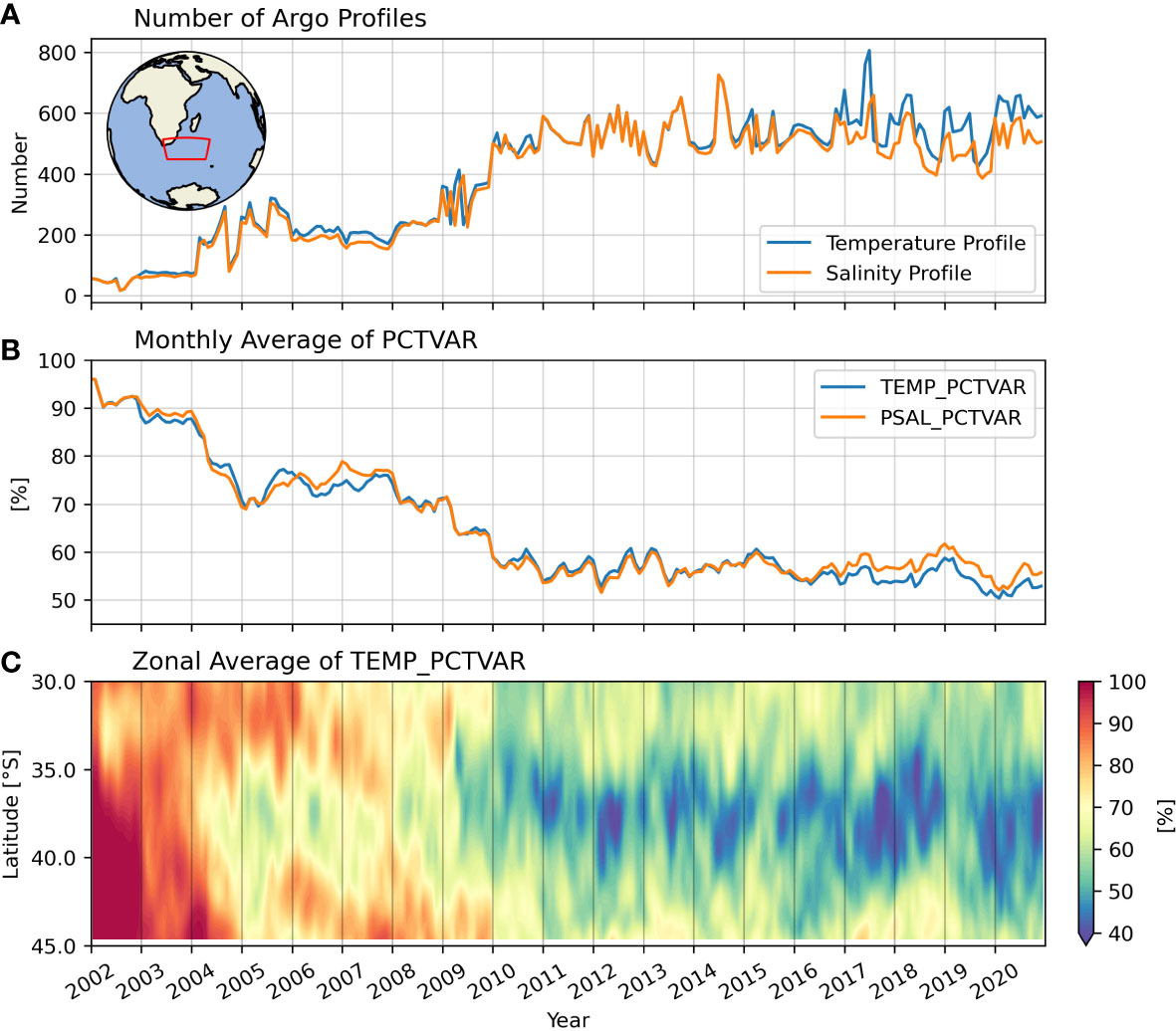
Figure 1 (A) Temperature (blue) and salinity (orange) profiles in the Southwest Indian Ocean subtropical gyre for each month. The red box in the inset map (20–60°E, 30–45°S) indicates the region from which the profiles were calculated. (B) Monthly mean of a priori variance (PCTVAR) for temperature (blue) and salinity (orange). (C) Zonal mean of PCTVAR for each month. Both (B) and (C) were calculated in the same region as (A). The number of Argo profiles and PCTVAR parameters were obtained from the ISAS20 dataset.

To compute the total heat flux, we used the Objectively Analyzed Air–Sea Fluxes (OAFlux; Yu et al., 2008) monthly latent and sensible heat dataset combined with surface radiative flux data from the Clouds and the Earth’s Radiant Energy System (CERES) project (Kato et al., 2018). We utilized the Energy Balanced and Filled (EBAF)-Surface product as an appropriate means by which the net radiative heat flux emitted from the ocean may be determined. We examined data obtained during the period from 2005 to 2020. All previously mentioned datasets were transformed onto a 0.5° grid using the Python package xESMF (Zhuang, 2018). For the OAFlux and CERES datasets, bilinear interpolation was applied, whereas for the ISAS20 gridded fields, a conservative interpolation method was employed. We utilized the Gibbs-SeaWater (GSW) Oceanographic Toolbox (McDougall and Barker, 2011) to compute density. All computations and data processing were performed using the xarray package (Hoyer and Hamman, 2017; Hoyer et al., 2023).

2.2 Decomposition of net heat flux and latent heat

To understand the primary reason for the heat flux anomaly, we analyzed each component of the net heat flux. Net heat flux (Qnet) was calculated as follows:

$\begin{array}{ll}\begin{array}{c}Qnet=SW+LW+LH+SH\end{array}& (1)\end{array}$

where SW is shortwave radiation, LW is longwave radiation, LH is latent heat, and SH is sensible heat. A positive value of the net heat flux and its components indicates that heat is released from the ocean to the atmosphere (positive upward). Furthermore, we decomposed the latent heat (LH) anomaly to examine its controlling factors, such as surface wind speed and humidity, and LH anomalies were decomposed based on the following equation (following Tanimoto et al., 2003 and Takahashi et al., 2021):

$\begin{array}{ll}\begin{array}{c}L{H}^{\prime }= {\rho }_{a}L{C}_e[\overline{U_a}(q_s^{\text{'}}-q_a^{\text{'}})+ U_a^{\text{'}}(\overline{q_{s }}-\overline{q_a})+U_a^{\text{'}}(q_s^{\text{'}}-q_a^{\text{'}})-\overline{U_a^{\text{'}}(q_s^{\text{'}}-q_a^{\text{'}})}]\end{array}& (2)\end{array}$

where ρ_a is atmospheric density, L is latent heat of vaporization, C_e is the bulk coefficient, U_a is wind speed at 10 m above the sea surface, q_s is specific humidity at the sea surface, and q_a is specific humidity 2 m above the sea surface. The overbar indicates the climatological mean for each month, whereas the prime denotes the anomaly from the mean. The first term on the right-hand side (RHS) of the equation represents the contribution of differences in specific humidity at the sea surface and humidity at a height of 2 m (q′ = $q_s^{\text{'}}-q_a^{\text{'}}$), while the second term represents the contribution of anomalous wind speed at 10 m height (($U_a^{\text{'}}$). The third term describes the combined effect of changes in wind speed anomaly and humidity difference anomaly ($U_a^{\text{'}}$q′), and the fourth term is the monthly climatology of the third term. The last two terms have very small values and can therefore be disregarded.

2.3 Potential vorticity and brunt Vaisala frequency

A mode water is distinguished by a layer with low stratification, and there are two commonly used approaches to assess its vertical stratification: vertical temperature gradient (dT/dz) and potential vorticity (PV). Potential vorticity is defined as follows:

$\begin{array}{ll}\begin{array}{c}PV=-\frac{f}{\rho }\frac{\partial \sigma }{\partial z}\end{array}& (3)\end{array}$

where f is the Coriolis parameter, ρ is in situ density, and σ is potential density. Relative vorticity was deemed negligible since it is much smaller than planetary vorticity. We calculated the vertical potential density gradient (dσ/dz) by taking the potential density difference between adjacent grid points above and below (with a depth difference of 10 m). We used the same approach to compute the vertical temperature gradient (dT/dz), where T represents potential temperature.

To examine the upper layer stratification in summer, we used the Brunt-Vaisala frequency squared (N²) as a proxy of stratification. N² is calculated as follows:

$\begin{array}{ll}\begin{array}{c}{N}^2=\frac{g}{\rho }\frac{\partial \sigma }{\partial z}\end{array}& (4)\end{array}$

where N is the Brunt-Vaisala frequency, g is the acceleration due to gravity, ρ is in situ density, and σ is potential density.

3 Results

3.1 September mixed layer

We defined the MLD as the depth at which the density increases by 0.125 kg m⁻³ and the temperature changes by 0.5°C relative to the surface, with temperature and density values at 10 m considered as the surface values. The MLD was determined as the shallowest depth calculated between the two definitions at each grid point. Using only temperature as a criterion to determine MLD can lead to overestimation in areas of strong salinity stratification. Similarly, relying solely on density criteria can result in overestimation in the region of compensated layers, where the density is vertically uniform, while the temperature and salinity change rapidly with depth (de Boyer Montégut et al., 2004; Oka et al., 2007). To avoid such potential overestimation, we utilized a combination of temperature and density criteria, taking advantage of the temperature and salinity data provided by the Argo float system.

The MLD distribution in September is shown in Figure 2A. September was selected because it represents the late winter period when the MLD is deepest. The dense mixed layer temperature contours around 40°S indicate the presence of the Agulhas Return Current. As shown in Figure 2A, thick mixed layers are observed on the equatorial flank of the Agulhas Return Current. The red dashed box in Figure 2A represents the formation region of IOSTMW. We intentionally excluded the coast of South Africa and the Agulhas Current region because we found that winter heat loss and variability in summer stratification in these areas were not clearly associated with the formation of IOSTMW formation. The characteristics of the winter mixed layer play a crucial role in the study of IOSTMW. During the spring, the seasonal thermocline forms and caps these deep winter mixed layers, resulting in the formation of IOSTMW. The properties of the winter mixed layer are important because they are closely tied to those of IOSTMW. This newly formed IOSTMW is then transported away from its formation zones, leaving behind a distinctive signature of winter mixing across vast regions of the Indian Ocean subtropical gyre.

FIGURE 2

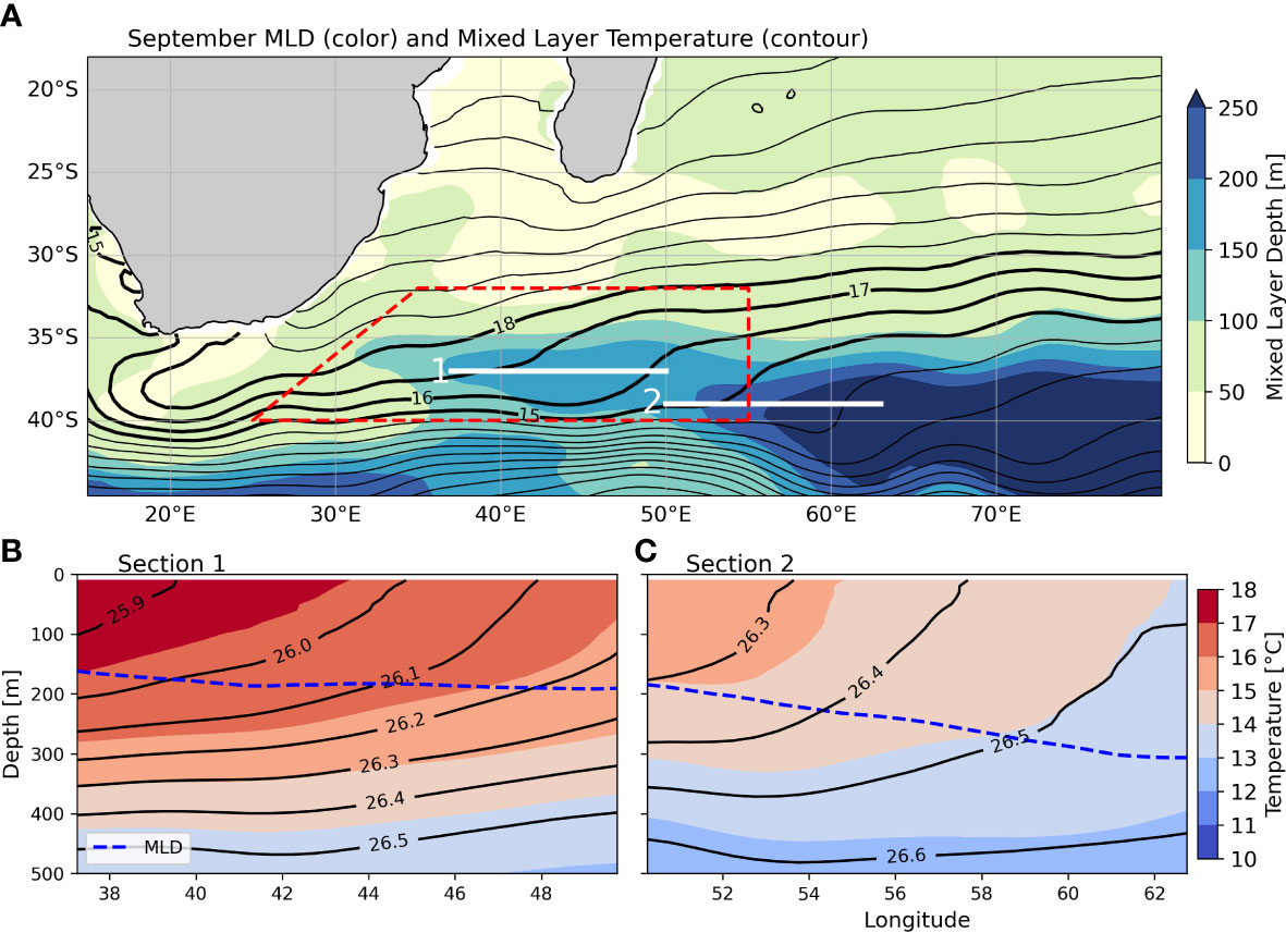
Figure 2 (A) The distribution of the MLD (color) against mixed layer temperature (contour) in September. The red dashed box indicates the formation region of IOSTMW used in this study. The white lines indicate zonal sections shown in (B, C). (B) Vertical profile at the zonal section at 37°S, from 37–50°E. Colors represent the temperature, contours represent potential density, and the blue dashed line is the mixed layer depth (MLD). (C) As in (B) but from the zonal section at 39°S, from 50–63°E.

Figures 2B, C shows the properties of the deep winter mixed layer north of the Agulhas Return Current. According to Tsubouchi et al. (2010), IOSTMW is estimated to have a temperature range of 16°C–17°C and a density range of 25.9–26.1 σ_θ, while Feucher et al. (2019) found that the average temperature of IOSTMW lies between 16.5°C–17.8°C with an average density of 25.9–26.0 σ_θ. Although the results of these studies may vary slightly, they are nonetheless within the range of mixed layer properties presented in Figure 2A, suggesting that the IOSTMW is linked to the late winter mixed layer. In this study, we excluded the deep mixed layers located east of 55°E with a temperature below 15°C and a density greater than 26.4 σ_θ. These properties of this water mass bear greater similarity to the lighter variants of Subantarctic Mode Water (SAMW), as described in prior studies (Fine, 1993; Wong, 2005; Koch-Larrouy et al., 2010).

3.2 Definition of the IOSTMW

3.2.1 The impact of using different definitions

In previous studies, the IOSTMW has been defined in various ways. Ma et al. (2016) defined it as a layer with a density of 25.8–26.2 σ_θ, and a potential vorticity (PV)< 2 × 10⁻¹⁰ m⁻¹ s⁻¹, Ma and Lan (2017) defined it as a layer with a temperature of 15.5°C–17.5°C and PV< 1.5 × 10⁻¹⁰ m⁻¹ s⁻¹, and lastly, Jiang et al. (2022) defined IOSTMW as a layer with a temperature of 15.5°C–17.5°C, a density of 25.8–26.2 σ_θ, and a PV< 2 × 10⁻¹⁰ m⁻¹ s⁻¹. It is important to note that Tsubouchi et al. (2010) and Feucher et al. (2019) did not use a single definition to detect IOSTMW. Tsubouchi et al. (2010) used variations in dT/dz for each profile, whereas Feucher et al. (2019) adopted the Objective Algorithm for the Characterization of the Permanent Pycnocline (OAC-P), developed by Feucher et al. (2016), to determine the global properties of mode waters using Argo profiles. In this section, we will discuss the importance of defining IOSTMW in light of the various definitions used in past studies.

Previous studies concerning North Atlantic Subtropical Mode Water (NASTMW) have highlighted the significance of accurately defining mode waters. For example, Forget et al. (2011) compiled estimates of eighteen-degree water and subtropical mode water volumes, annual formation, and amplitudes of seasonal cycles from past studies (see their Table 2), showing that water mass definitions can be a significant source of confusion in volume estimates, as their estimates can be highly sensitive to subtle differences in definition. In particular, they showed that adding potential vorticity restrictions (PV< 1.5 × 10⁻¹⁰ m⁻¹ s⁻¹ and PV< 0.2 × 10⁻¹⁰ m⁻¹ s⁻¹) leads to changes in the amplitude of the seasonal cycle. Peng et al. (2006) also examined the range of definitions used to define NASTMW, finding that using an excessively strict vertical temperature gradient (dT/dz) to define NASTMW could exclude older mode water with higher stratification, and may impact the spatial and temporal evolution of STMW properties. Conversely, using too relaxed dT/dz could lead to the inclusion of water masses that are not well mixed as part of the mode water. Peng et al. (2006) therefore concluded that a dT/dz of< 1°C/100 m is the most suitable restriction to define NASTMW among all restrictions examined. Building upon their insights, we similarly assessed how different definitions could potentially influence the properties of IOSTMW.

Figure 3 shows the temperature, density, PV, and dT/dz profiles from an Argo float that captures the signal of the IOSTMW. In Figure 3, the IOSTMW layers identified using various criteria are represented alongside each of these variables. We focused on the 15°C–18°C range based on the mixed layer temperature shown in Figure 2, and used various PV and dT/dz values as restrictions to define the IOSTMW layer. We elected to include 15°C because a thick MLD with a temperature of 15°C can clearly be observed between 50–52°E (Figure 2C).

FIGURE 3

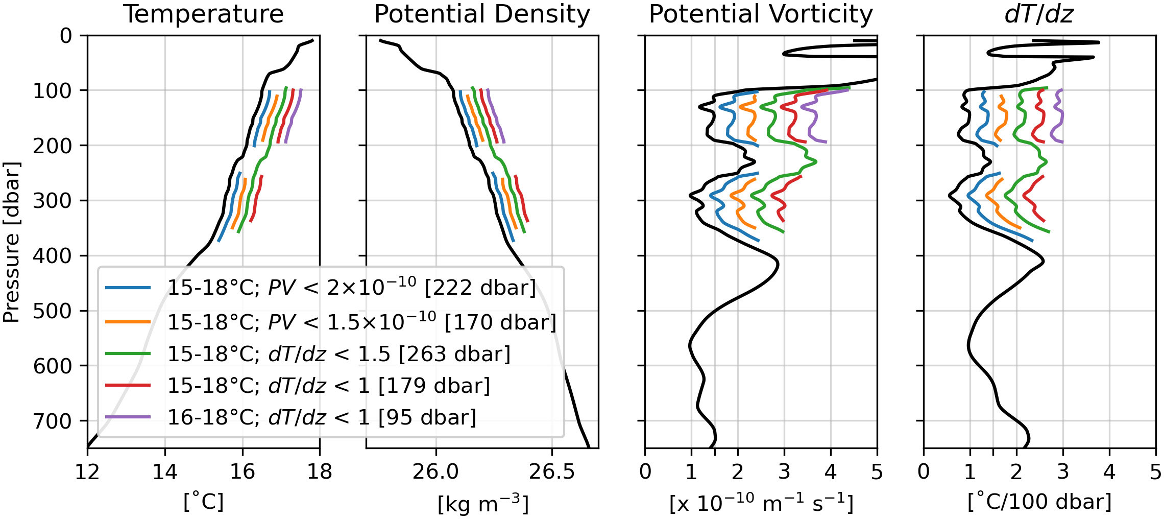
Figure 3 Argo profile (float ID 1901377, recorded at 37.9°S and 45°E on 2011-12-18) in the formation region of IOSTMW that captures the signal of IOSTMW [following Figure 2.8 in Maze (2020)]. Layers of IOSTMW using various definitions are drawn alongside each profile. The number inside the bracket denotes the IOSTMW thickness for each definition.

Figure 3 displays that the characteristics of the IOSTMW layer are significantly influenced by the criteria by which it is defined. The blue and orange lines, representing PV-restricted definitions, reveal that the IOSTMW layer is divided at 200–250 dbar due to the presence of a PV > 2 × 10⁻¹⁰ m⁻¹ s⁻¹ layer in that region, as evident from the PV profile. However, this separation is not visible when using a dT/dz< 1.5°C/100 dbar definition (green line). The difference between the PV and dT/dz restrictions could be attributed to the fact that PV is also affected by the salinity gradient, which could contribute to locally increased PV at 200–250 dbar. When we compare the thickness of the two PV-restricted definitions (blue and orange lines), we find a difference of approximately 50 dbar, whereas reducing the dT/dz< 1.5°C/100 dbar (green line) to dT/dz< 1°C/100 dbar (red line) yields a thickness difference of approximately 80 dbar. These differences are noteworthy, particularly since Feucher et al. (2019) reported an average thickness of 135 m for the IOSTMW layer. We also examined the impact of modifying the temperature range in the dT/dz< 1°C/100 dbar restriction, selecting only temperatures from 16°C–18°C (purple line). When comparing the purple line against the red line, it is clear that narrowing or expanding the temperature range could have a significant effect on the mean properties of the IOSTMW layer.

Figure 3 illustrates the means by which the definition of mode water can significantly impact the results of a study. There is no single, universally accepted definition for each mode water; rather, the definition used in each study depends on its research objectives. The main objective of this study is to identify the layers of IOSTMW that are most strongly affected by winter heat loss. We hypothesize that the properties of subducted IOSTMW can serve as a useful indicator of winter heat loss intensity, provided that we carefully select the layers that are influenced by this process. Therefore, we examined various temperature ranges and stratification restrictions to determine the most suitable definition for this purpose. We also investigated the impact of summer stratification on IOSTMW formation. Stratification during the summer and fall seasons is crucial because it sets the stage for the formation of the convective mixed layer in the following cooling season (Qiu and Chen, 2006). This factor has been known to hinder or facilitate the formation of a thick STMW in other ocean basins (e.g., Qiu and Chen, 2006; Li et al., 2022).

3.2.2 The most suitable definition

In our study, we explored different definitions of IOSTMW to identify the one that is most closely related to winter heat loss. Figure 2A illustrates the expanded contours of mixed layer temperature within the formation region (red dashed line) ranging from 15°C–18°C, which provides optimal conditions for mode water formation. We then evaluated four IOSTMW definitions, namely: (1) dT/dz< 1.5°C/100 m with a temperature range of 15°C–18°C, (2) dT/dz< 1.5°C/100 m with a temperature range of 16°C–18°C, (3) dT/dz< 1°C/100 m with a temperature range of 15°C–18°C, and (4) dT/dz< 1°C/100 m with a temperature range of 16°C–18°C. We did not include potential vorticity (PV) as a restriction, following the recommendation of Tsubouchi et al. (2010) to use dT/dz instead. According to their results, density compensation can be observed across a range of densities, including those of the IOSTMW. Furthermore, to acquire a more robust detection of the IOSTMW layer, we eliminated IOSTMW layers with thickness less than 40 m. To investigate the correlation between IOSTMW and winter heat loss and summer stratification, we calculated the correlation coefficient between the mean thickness of the IOSTMW in late winter (September) for each year and both the net heat flux during winter (June–August) and the upper layer stratification (0–150 m) in summer (January–February). These calculations were performed in the formation region of IOSTMW, which is marked by the red dashed box in Figure 2.

Figure 4 demonstrates that definitions with dT/dz< 1°C/100 m show a stronger correlation with winter heat loss, with a significance level greater than 99%. This suggests that the older layer, which is located at a greater depth below the weakly stratified layer, is not a result of winter heat loss in the same year, and contains properties that differ from the newly formed IOSTMW. Regarding the impact of summer stratification on the formation of subtropical mode water, previous studies (e.g., Qiu and Chen, 2006; Li et al., 2022) have shown that a less (more) stratified water column in the summer or fall promotes (inhibits) the deep formation of the mixed layer, which directly affects the thickness of the subtropical mode water. Although an anticorrelation is expected between IOSTMW thickness and summer stratification, only definitions with temperatures of 16°C–18°C show negative correlation coefficients in Figure 4. The definition of dT/dz< 1°C/100 m with a temperature range of 16°C–18°C exhibits the relatively best correlation among all the tested definitions. Including the 15°C layer decreases the correlation coefficient as a result of the depth limit chosen when averaging N² in summer. We selected a depth limit of 150 m based on the typical depth of the deep mixed layer in the region of formation (Figure 2), allowing us to focus on the impact of summer stratification on the development of the deep mixed layer. However, except for east of 50°E, the 15°C–16°C layers are generally located deeper than the mixed layer depth, whereas the 16°C–18°C layer is primarily included in the mixed layers in most regions (Figures 2B, C). Consequently, including the 15°C–16°C layers reduces the correlation coefficient. We also examined the effect of changing the lower depth limit to 200 m, but the results were not significantly different. It is important to note that these results do not necessarily suggest that the formation of the 15°C–16°C IOSTMW layer is unrelated to the breaking of summer/fall stratification. Rather, the choice of stratification depth and research domain in this study is more appropriate for analyzing the 16°C–18°C IOSTMW layer. Figure 2 clearly demonstrates that the depth of the mixed layer significantly increases east of 50°E. Hence, including the 15°C–16°C layer may require a different research domain and a distinct depth for the summer stratification layer.

FIGURE 4

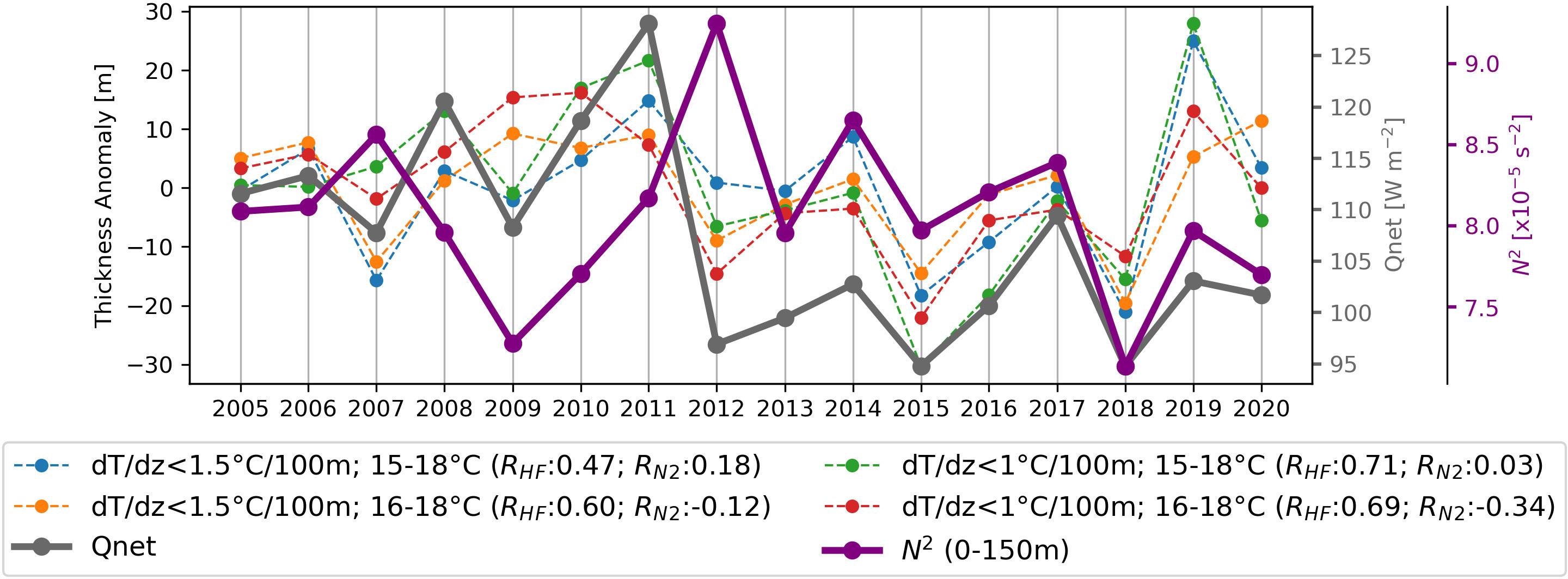
Figure 4 Interannual variability in thickness anomaly according to each examined definition. Blue, orange, green, and red dashed lines represent IOSTMW as defined using definitions (1), (2), (3), and (4), respectively. Thick gray line indicates winter (June–August) net heat flux; thick purple line indicates summer (January–March) stratification of the upper layer (0–150 m). R_HF denotes the correlation coefficient between the thickness variability of each definition with the winter heat flux, and R_N2 denotes the correlation coefficient between the thickness variability of each definition with summer stratification.

Figure 4 shows that the IOSTMW layer defined as a layer with dT/dz< 1°C/100 m and a temperature of 16°C–18°C (red line in Figure 4) exhibits the highest correlation coefficients with winter heat flux and generally correlates with summer stratification among all definitions. Therefore, we defined the IOSTMW layer using that definition in order to explain the mechanisms behind its year-to-year variability and to evaluate the combined influences of winter heat flux and summer stratification in determining the thickness of IOSTMW in late winter.

3.3 Mechanisms of the interannual variability: Winter heat loss and summer stratification

Figure 5 displays scatter plots of IOSTMW thickness in September plotted against surface heat flux during winter (June–August) (Figure 5A) and summer (January–March) N² values from the surface to 150 m (Figure 5B). Figure 5A shows that the thickness of IOSTMW is lowest in 2018, 2012, and 2015; this can be attributed to weak heat loss during those years. However, summer stratification varied significantly over these years. 2012 exhibited a high stratification, which is expected to inhibit the formation of a thick IOSTMW layer. In contrast, 2015 exhibited a relatively low stratification, whereas 2018 had the lowest summer stratification among all the data evaluated in Figure 5B. 2015 and 2018 share a notable common characteristic: they have the weakest winter heat loss among all the years examined. Hence, this finding suggests that even if summer stratification is weak, a thick IOSTMW cannot form in late winter if the winter heat loss is extremely weak. On the other hand, the year 2011 featured strong heat loss, but its summer stratification was well-stratified, which could have hindered the formation of a thick mode water layer. The years 2009, 2010, and 2019 are examples of thick years for IOSTMW, which provide insight into how summer stratification and winter heat loss combine to influence the formation of IOSTMW. In 2019 and 2009, moderate heat loss with weak summer stratification resulted in the formation of thick mode waters. The year 2010 exhibited both intense heat loss and weak summer stratification, naturally leading to the formation of thick mode water during late winter. These examples illustrate how winter heat loss and summer stratification work together to form IOSTMW each year. However, the cases of years 2015 and 2018 highlight that winter heat loss is the primary factor determining the IOSTMW thickness. Although a poorly stratified upper layer is favorable for the formation of a thick IOSTMW, extremely weak heat loss makes it difficult for a thick IOSTMW layer to form.

FIGURE 5

Figure 5 Scatter plots showing (A) September IOSTMW thickness against winter net heat flux. Color represents the summer stratification. R- and p-values are calculated between the September thickness and winter heat flux (B) September thickness of IOSTMW against the summer stratification. The color represents the winter heat flux. The R- and p-value are calculated between the September thickness and summer stratification. Error bars in both figures denote the 95% confidence interval. The correlation coefficients and the 95% confidence interval were calculated using the SciPy package (Virtanen et al., 2020).

4 Discussion

4.1 Net heat flux and latent heat anomaly decomposition

In the previous section, we showed that winter heat loss is the primary factor responsible for determining the annual thickness of IOSTMW. In this section, we explore in more detail how winter heat loss contributes to the formation of IOSTMW. To begin, we break down the net heat flux into its components, as illustrated in Figure 6A. It is noticeable that in some years, sensible heat (represented by the dashed light blue line) and latent heat (dashed dark-blue line) work together to produce an anomalous heat flux, such as observed in 2008, 2010, 2011, and 2018. However, we found that, in 2012 and 2015, latent heat alone was responsible for anomalous weak winter heat loss. We therefore further investigated the variability in latent heat.

FIGURE 6

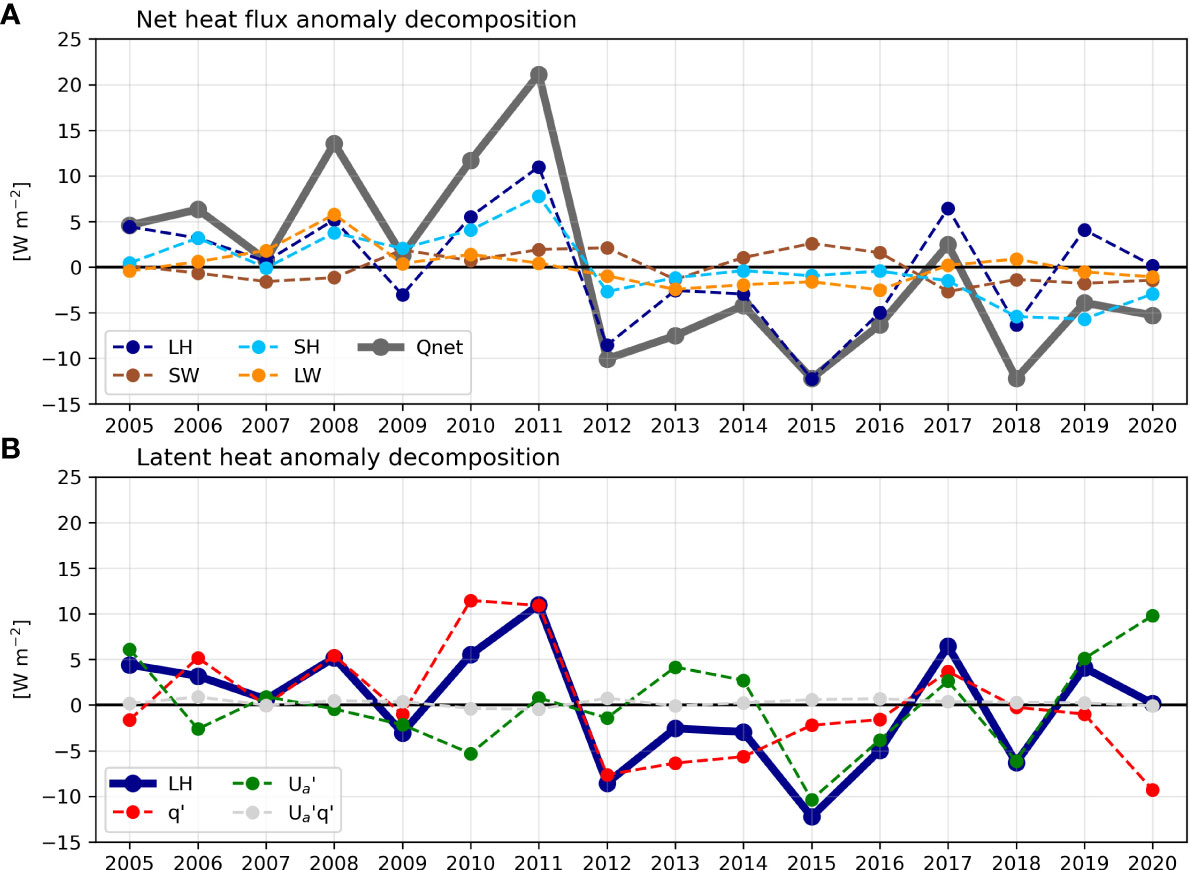
Figure 6 (A) Decomposition of the winter net heat flux anomaly. Dashed dark-blue line represents the contribution from the latent heat anomaly (LH), dashed light blue line represents the contribution from the sensible heat anomaly (SH), dashed brown line represents the contribution from shortwave radiation (SH), dashed orange line represents the contribution from longwave radiation (LH), and solid thick gray line denotes net heat flux. (B) Decomposition of the latent heat anomaly. Solid thick dark-blue line denotes the latent heat anomaly (LH), dashed red line is the contribution from the humidity difference anomaly (q’ = q_s’-q_a’), dashed green line is the contribution from wind speed at the 10 m height anomaly (U_a’), and dashed light gray line denotes the combined effects of q’ and U_a’.

Figure 6B presents the time series of the first three LH components on the RHS of Equation 2, highlighting that the three thinnest years of IOSTMW are caused by different factors. Specifically, the thin IOSTMW in 2012 is the result of an anomalously small humidity difference at the sea surface and at a height of 2 m, whereas the thin IOSTMWs in 2015 and 2018 are due to anomalously weak wind speed over the formation region. Conversely, the thick IOSTMW in 2010 was the consequence of a large difference in humidity leading to a strong winter heat loss. However, the wind was anomalously weak in 2010, resulting in decreased total latent heat. These findings demonstrate that thin IOSTMW years are associated with anomalously weak latent heat flux.

4.2 Composite analysis of the thick and thin years

Furthermore, to elucidate the formation of the thick and thin years, we selected years wherein the mean thickness value exceeds 1 standard deviation (σ = 10.35 m; standard deviation calculated from thickness anomaly timeseries). The thick years include 2009, 2010, and 2019, while thin years include 2012, 2015, and 2018. Figure 7 displays the average winter net heat flux and summer stratification for both the thick and thin years. Figure 7B reveals a negative anomaly in the net heat flux, which indicates a weak heat loss during the thin years. In contrast, the formation region of IOSTMW, particularly east of 40°E, experiences intense heat loss during thick years (Figure 7A). However, this strong heat loss distribution is not as prominent as the weak heat loss distribution observed during thin years because the net heat loss during 2009 and 2019 is not particularly strong, as seen in Figures 4, 6. During these years, the formation of thick IOSTMW layers is aided by the weakly stratified upper layer during the summer season, as shown in Figure 7C. In thin years, the summer average N² shows a positive anomaly value inside the formation region (Figure 7D). However, it is important to note that this is mainly due to the averaging process. The negative anomaly value during the thick years (Figure 7C) is due to the relatively weak summer stratification for 2009, 2010, and 2019 (Figure 5). On the other hand, during the thin years, there appears to be an inconsistency between the weak stratification in 2018 and the very well-stratified summer of 2012 (Figure 5). The presence of thin IOSTMW layers during thin years is attributed to the extremely weak winter heat loss, as indicated in section 4.1.

FIGURE 7

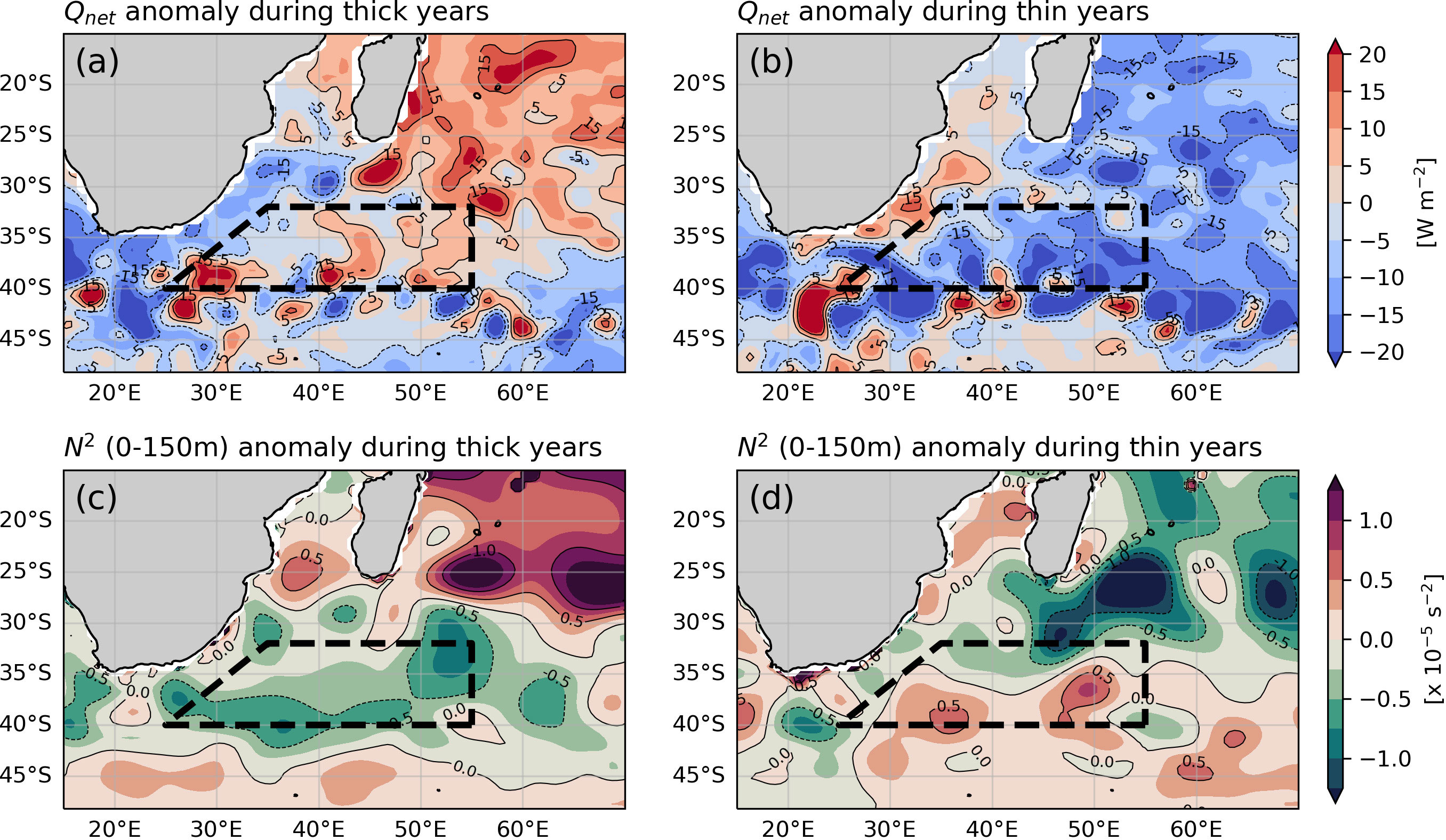
Figure 7 Winter net heat flux anomaly averaged for (A) thick years (2009, 2010, and 2019), and (B) thin years (2012, 2015, and 2018). Summer N² anomaly averaged from 0–150 m during (C) thick years and (D) thin years. Solid (dashed) contours represent positive (negative) values in both the upper and lower panels.

To better understand the impact of anomalous latent heat on the heat flux anomaly, Figure 8 displays the spatial distribution of $U_a^{\text{'}}$ and ($q_s^{\text{'}}-q_a^{\text{'}}$) calculated using Equation 2. During thin years, the wind speed distribution shows a weak anomaly (Figure 8B) coupled with an anomalously small difference in humidity between the sea surface and the air (Figure 8D). This combination provides the ideal conditions for creating an anomalously thin IOSTMW layer. Figure 6 demonstrates that the latent heat anomaly contributions from the wind speed ($U_a^{\text{'}}$) and humidity difference ($q_s^{\text{'}}-q_a^{\text{'}}$) have negative values for 2012, 2015, and 2018, i.e., weakened heat loss from the ocean to the atmosphere. On the other hand, the opposing effects of the wind and humidity contributions during thick years can be observed (Figure 8A, C). This can be explained by examining the latent heat decomposition in Figure 6B. In particular, the wind contribution in 2019 has a positive effect on latent heat, enhancing heat loss to the atmosphere, but this is counteracted by the negative wind contribution in 2009 and 2010 (green dashed line in Figure 6B). Therefore, the distribution of the wind speed anomaly is weakly negative (Figure 8A). In Figure 8C, a positive anomaly value in the humidity difference suggests an intense heat loss to the atmosphere. The ($q_s^{\text{'}}-q_a^{\text{'}}$) anomalies in 2009 and 2019 are small and close to zero, as shown by the red dashed line in Figure 6B. Therefore, the remaining positive contribution observed in 2010 dominates when averaging the three thick years, showing positive anomalies around the formation region.

FIGURE 8

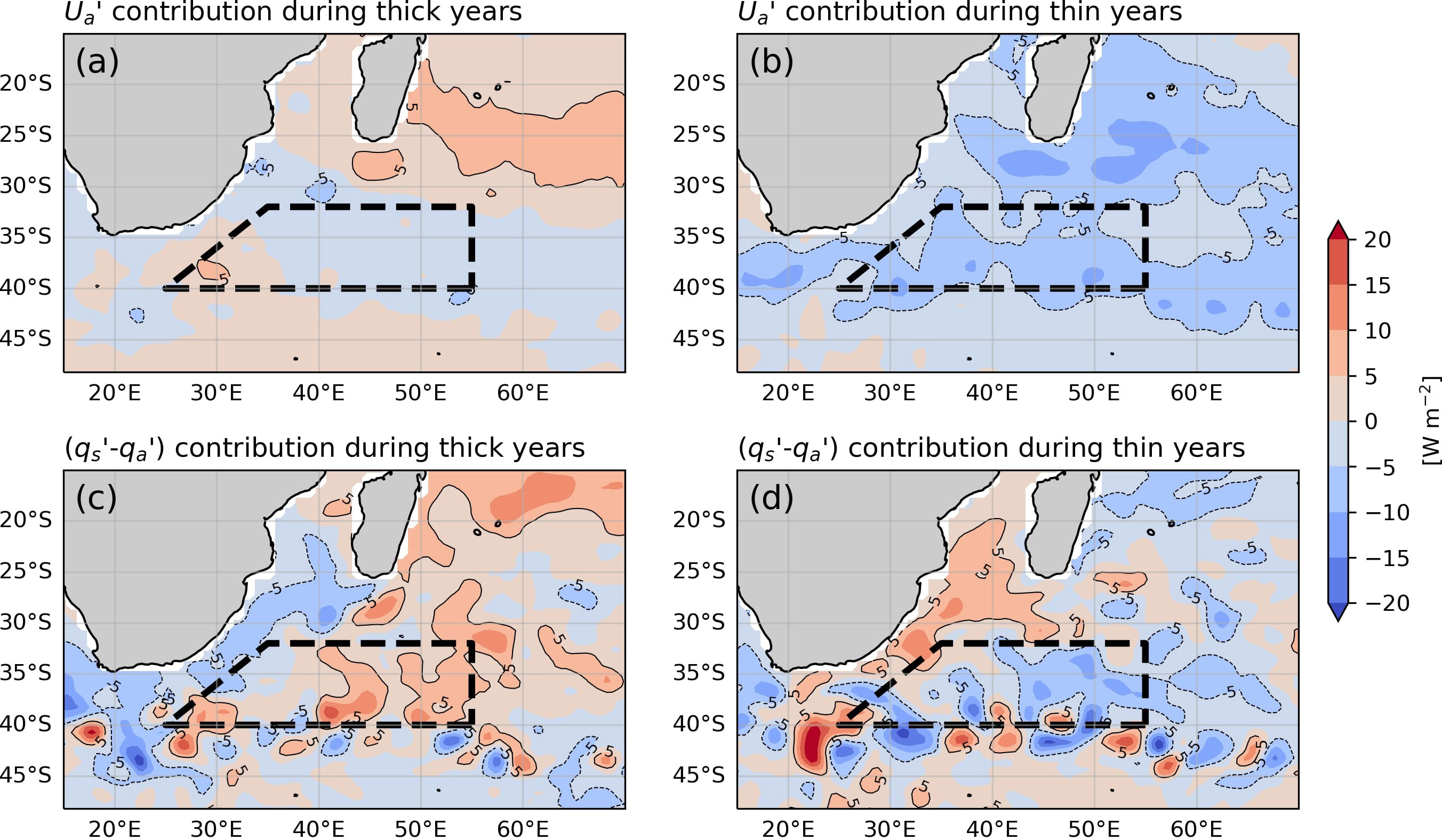
Figure 8 U_a’ contribution to the latent heat anomaly averaged during (A) thick years (2009, 2010, and 2019) and (B) thin years (2012, 2015, and 2018) and the q_s’-q_a’ contribution averaged during (C) thick years and (D) thin years. Solid (dashed) contours represent positive (negative) values in both the upper and lower panels.

The lower panels of Figure 8 display a similar pattern to that shown in the upper panels of Figure 7, indicating the significant role played by ($q_s^{\text{'}}-q_a^{\text{'}}$) in the total winter heat flux. During thin years, the negative contribution from ($q_s^{\text{'}}-q_a^{\text{'}}$) is further augmented by the negative contribution from $U_a^{\text{'}}$, resulting in a weak net heat loss anomaly. Figure 6B shows that the latent heat anomaly is the primary cause of the weak heat loss, with the exception of 2018, when sensible heat also exhibited a negative contribution. These findings demonstrate how ($q_s^{\text{'}}-q_a^{\text{'}}$) and $U_a^{\text{'}}$ combine to engender a weak heat loss anomaly, which hinders the formation of thick IOSTMW. Conversely, during thick years, ($q_s^{\text{'}}-q_a^{\text{'}}$) displays positive anomalous values (Figure 8C) but is slightly counteracted by the contribution of $U_a^{\text{'}}$ (Figure 8A). However, the net heat flux values are similar or greater at some locations within the formation region (Figure 7A), implying that other contributions from net heat flux components are also present. During the thick years, contributions from $U_a^{\text{'}}$ and ($q_s^{\text{'}}-q_a^{\text{'}}$) act in opposition (e.g., 2010 and 2019 in Figure 6B); as such, the total latent heat anomaly is not strongly positive.

5 Summary and conclusions

This study aimed to investigate the temporal variability of IOSTMW using Argo profiles in the Southwest Indian Ocean. Previous data scarcity made it challenging to study the IOSTMW, leading to studies reliant on models and climatologies. Using the ISAS20 data product, based solely on Argo profiles, we were able to analyze the September mixed layer properties, which aligns with IOSTMW properties reported in previous studies. Because different definitions of IOSTMW have been used in the past, we sought to determine the most suitable definition for this study. Specifically, we sought the definition that is most sensitive to winter heat loss. Of the four definitions examined, we found that the year-to-year thickness of the IOSTMW defined as a layer with dT/dz< 1°C/100 m and a temperature range of 16°C–18°C exhibits the best correlation with winter heat loss. Additionally, we investigated how summer stratification in the upper layer (0–150 m) could potentially affect the formation of IOSTMW each year. Our analysis revealed that the year-to-year mean IOSTMW thickness in September is strongly correlated with winter heat loss (R: 0.69, p: 0.002); however, the correlation between IOSTMW thickness and summer stratification is relatively low (R: −0.34, p: 0.20). It is important to note that the low correlation coefficient is mainly attributed to the two years with anomalously low winter heat loss.

Our findings demonstrate that summer stratification and winter heat loss work together in determining the thickness of IOSTMW in late winter each year, and are summarized in Figure 9, which is based on 16 years of data as shown in Figure 5. These results indicate that although summer stratification may be weak, the formation of thick mode water is hindered if winter heat loss is inadequate to deepen the mixed layer. We also found that years in which IOSTMW layers are thick tend to be preceded by weak summer stratification, suggesting that the poorly stratified upper layer in summer or spring sets the stage for the formation of thick IOSTMW in late winter, provided that there is sufficient winter heat loss. On the other hand, intense winter heat loss does not necessarily guarantee the formation of thick IOSTMW, because summer stratification can hinder the convective mixing process. Overall, our results suggest that while winter heat loss is the primary factor determining the thickness of IOSTMW each year, summer stratification plays an important role in facilitating or hindering the formation of thick IOSTMW. Comparing our results with previous studies, the work of Qiu and Chen (2006) explored the impact of winter heat loss and summer stratification on mixed layer formation in the North Pacific. They emphasized the greater importance of summer stratification in determining the thickness of winter mixed layers in that region. In contrast, our results align more closely with the study by Li et al. (2022) conducted in the North Atlantic, where we observed that winter heat loss has a more dominant influence on determining the thickness of IOSTMW compared to summer stratification.

FIGURE 9

Figure 9 Schematic diagram illustrating the combined influences of summer stratification and winter heat loss on the thickness of IOSTMW in late winter, based on the results presented in Figure 5.

Furthermore, we conducted a deeper analysis of winter heat loss variability by examining the individual components of the net heat flux. This investigation revealed that the latent heat anomaly plays a crucial role in determining the strength of heat loss in winter. In addition, we further analyzed the latent heat anomaly by breaking it down into its components to identify the most significant factors contributing to heat loss anomalies in the IOSTMW formation region. To focus on the formation of thick and thin mode waters, we analyzed the years in which the mean thickness anomaly exceeded one standard deviation according to the year-to-year thickness anomaly timeseries. We identified 2009, 2010, and 2018 as years characterized by a thick IOSTMW, whereas 2012, 2015, and 2018 were found to be years in which the IOSTMW was extremely thin. Our analysis indicated that years with thin IOSTMW layers were associated with anomalously negative contributions from both the humidity difference anomaly ($q_s^{\text{'}}-q_a^{\text{'}}$) and wind speed anomaly $U_a^{\text{'}}$. These factors were determined to be the primary reasons for the anomalously weak heat loss in 2012, 2015, and 2018, hindering IOSTMW formation. Conversely, we found that the formation of thick IOSTMW was not accompanied by anomalously strong heat loss; rather, it was aided by weak summer stratification. The results of our latent heat decomposition analysis revealed that ($q_s^{\text{'}}-q_a^{\text{'}}$) opposed $U_a^{\text{'}}$ during thick years, reducing the magnitude of the latent heat anomaly and further lowering the intensity of heat loss. In summary, our study indicates that the primary cause of thin IOSTMW layers is extremely weak winter heat loss due to anomalously weak $U_a^{\text{'}}$ and ($q_s^{\text{'}}-q_a^{\text{'}}$), whereas the formation of a thick IOSTMW is aided by weak summer stratification.

Finally, it is important to note that the properties and temporal variability of mode water are highly sensitive to how it is defined. In our study, we focused on the IOSTMW layer that is most closely connected with the mixing generated by winter heat loss. There is no single best way to define a mode water; the most appropriate definition depends on the goals of a specific study. For the present study, we defined IOSTMW as the “young” IOSTMW layer that forms due to winter heat loss during the same year. This method is particularly useful for studying the mechanisms by which mode water captures anomalous winter mixing signals and transports them to the ocean interior via subduction.

Data availability statement

The data supporting the findings of this study can be found in online repositories. The ISAS20 temperature and salinity products were produced and distributed by the French Service National d'Observation Argo at LOPS and are available at https://www.seanoe.org/data/00412/52367/. CERES data were obtained from https://asdc.larc.nasa.gov/project/CERES/CERES_EBAF_Edition4.1. The global ocean heat flux and evaporation data were funded by the NOAA Climate Observations and Monitoring program and are available at https://oaflux.whoi.edu/data-access/. The code and processed datasets to reproduce all the figures in this study can be accessed at https://doi.org/10.5281/zenodo.7751277.

Author contributions

HA conducted the study and wrote the initial version of the paper. TS supervised the work and provided continuous scientific input and guidance throughout the writing process. All authors contributed to the article and approved the submitted version.

Funding

This work was supported by The International Joint Graduate Program in Earth and Environmental Sciences, Tohoku University (GP-EES), JSPS KAKENHI Grant JP19H05700, and JST SICORP Grant JPMJSC21E7. The open access publishing fee was supported by GP-EES and JSPS KAKENHI Grant JP19H05700.

Acknowledgments

The authors are grateful to the members of the Physical Oceanography Group at Tohoku University and Professors Bo Qiu, Kelvin Richards, and Niklas Schneider at the University of Hawai’i at Mānoa for their valuable contributions to this research. The meaningful discussions and suggestions provided by these individuals have greatly enriched the quality of our work.

Conflict of interest

The authors declare that the research was conducted in the absence of any commercial or financial relationships that could be construed as a potential conflict of interest.

The reviewer SH declared a shared affiliation with the author TS to the handling editor at the time of review.

Publisher’s note

All claims expressed in this article are solely those of the authors and do not necessarily represent those of their affiliated organizations, or those of the publisher, the editors and the reviewers. Any product that may be evaluated in this article, or claim that may be made by its manufacturer, is not guaranteed or endorsed by the publisher.

References

Argo Science Team (2001). Argo: the global array of profiling floats. observing the oceans in the 21st century.

Google Scholar

Backeberg B. C., Counillon F., Johannessen J. A., Pujol M. I. (2014). Assimilating along-track SLA data using the EnOI in an eddy resolving model of the agulhas system. En Ocean Dynam. 64 (8), 1121–1136. doi: 10.1007/s10236-014-0717-6

CrossRef Full Text | Google Scholar

Bernardo P. S., Sato O. T. (2020). Volumetric characterization of the south Atlantic subtropical mode water types. Geophys. Res. Lett. 47 (8), GL086653. doi: 10.1029/2019GL086653

CrossRef Full Text | Google Scholar

Bryden H. L., Beal L. M., Duncan L. M. (2005). Structure and transport of the agulhas current and its temporal variability. J. Oceanogr. 61 (3), 479–492. doi: 10.1007/s10872-005-0057-8

CrossRef Full Text | Google Scholar

de Boyer Montégut C., Madec G., Fischer A. S., Lazar A., Iudicone D. (2004). Mixed layer depth over the global ocean: an examination of profile data and a profile-based climatology. J. Geophys. Res. 109 (C12), (C12). doi: 10.1029/2004JC002378

CrossRef Full Text | Google Scholar

Fernandez D., Sutton P., Bowen M. (2017). Variability of the subtropical mode water in the southwest pacific. J. Geophys. Res.: Oceans 122 (9), 7163–7180. doi: 10.1002/2017JC013011

CrossRef Full Text | Google Scholar

Feucher C., Maze G., Mercier H. (2016). Mean structure of the north Atlantic subtropical permanent pycnocline from in situ observations. J. Atmospheric Oceanic Technol. 33 (6), 1285–1308. doi: 10.1175/JTECH-D-15-0192.1

CrossRef Full Text | Google Scholar

Feucher C., Maze G., Mercier H. (2019). Subtropical mode water and permanent pycnocline properties in the world ocean. J. Geophys. Res.: Oceans 124 (2), 1139–1154. doi: 10.1029/2018JC014526

CrossRef Full Text | Google Scholar

Fine R. A. (1993). Circulation of Antarctic intermediate water in the south Indian ocean. Deep Sea Res. Part I: Oceanographic Res. Pap. 40 (10), 2021–2042. doi: 10.1016/0967-0637(93)90043-3

CrossRef Full Text | Google Scholar

Forget G., Maze G., Buckley M., Marshall J. (2011). Estimated seasonal cycle of north Atlantic eighteen degree water volume. J. Phys. Oceanogr. 41 (2), 269–286. doi: 10.1175/2010JPO4257.1

CrossRef Full Text | Google Scholar

Gaillard F., Reynaud T., Thierry V., Kolodziejczyk N., von Schuckmann K. (2016). In situ–based reanalysis of the global ocean temperature and salinity with ISAS: variability of the heat content and steric height. J. Climate 29 (4), 1305–1323. doi: 10.1175/JCLI-D-15-0028.1

CrossRef Full Text | Google Scholar

Gordon A. L., Lutjeharms J. R. E., Gründlingh M. L. (1987). Stratification and circulation at the agulhas retroflection. Deep Sea Res. Part A. Oceanographic Res. Pap. 34 (4), 565–599. doi: 10.1016/0198-0149(87)90006-9

CrossRef Full Text | Google Scholar

Hanawa K., Talley L. D. (2001). “Chapter 5.4 mode waters,” in International geophysics, vol. 77. (Academic Press). doi: 10.1016/S0074-6142(01)80129-7

CrossRef Full Text | Google Scholar

Harris T. F. W., Van Foreest D. (1978). The agulhas current in march 1969. Deep Sea Res. 25 (6), 549–561. doi: 10.1016/0146-6291(78)90643-4

CrossRef Full Text | Google Scholar

Hoyer S., Hamman J. (2017). Xarray: ND labeled arrays and datasets in Python. J. Open Res. Softw. 5 (1). doi: 10.5334/jors.148

CrossRef Full Text | Google Scholar

Hoyer S., Roos M., Hamman J., Magin J., Cherian D., Fitzgerald C., et al. (2023). Xarray (Version v2023.02.0) [Software]. Zenodo. doi: 10.5281/zenodo.598201

CrossRef Full Text | Google Scholar

Jiang J., Shi J., Huang F. (2022). Quasi-biennial variability of Indian ocean subtropical mode water subduction driven by atmospheric circulation modes during the argo period. J. Climate 35 (13), 4085–4098. doi: 10.1175/JCLI-D-21-0509.1

CrossRef Full Text | Google Scholar

Kato S., Rose F. G., Rutan D. A., Thorsen T. J., Loeb N. G., Doelling D. R., et al. (2018). Surface irradiances of edition 4.0 clouds and the earth’s radiant energy system (CERES) energy balanced and filled (EBAF) data product. J. Climate 31 (11), 4501–4527. doi: 10.1175/JCLI-D-17-0523.1

CrossRef Full Text | Google Scholar

Kobayashi T., Suga T. (2006). The Indian ocean HydroBase: a high-quality climatological dataset for the Indian ocean. Prog. Oceanogr. 68 (1), 75–114. doi: 10.1016/j.pocean.2005.07.001

CrossRef Full Text | Google Scholar

Koch-Larrouy A., Morrow R., Penduff T., Juza M. (2010). Origin and mechanism of subAntarctic mode water formation and transformation in the southern Indian ocean. Ocean Dynam. 60 (3), 563–583. doi: 10.1007/s10236-010-0276-4

CrossRef Full Text | Google Scholar

Kolodziejczyk N., Llovel W., Portela E. (2019). Interannual variability of upper ocean water masses as inferred from argo array. J. Geophys. Res.: Oceans 124 (8), 6067–6085. doi: 10.1029/2018JC014866

CrossRef Full Text | Google Scholar

Kolodziejczyk N., Prigent-Mazella A., Gaillard F. (2021). ISAS temperature and salinity gridded fields. doi: 10.17882/52367

CrossRef Full Text | Google Scholar

Kwon Y. O., Riser S. C. (2004). North Atlantic subtropical mode water: a history of ocean-atmosphere interaction 1961-2000. Geophys. Res. Lett. 31 (19). doi: 10.1029/2004GL021116

CrossRef Full Text | Google Scholar

Li K., Maze G., Mercier H. (2022). Ekman transport as the driver of extreme interannual formation rates of eighteen degree water. J. Geophys. Res.: Oceans 127 (1), JC017696. doi: 10.1029/2021JC017696

CrossRef Full Text | Google Scholar

Ma J., Lan J. (2017). Interannual variability of Indian ocean subtropical mode water subduction rate. Climate Dynam. 48 (11-12), 4093–4107. doi: 10.1007/s00382-016-3322-1

CrossRef Full Text | Google Scholar

Ma J., Lan J., Zhang N. (2016). A study of Indian ocean subtropical mode water: subduction rate and water characteristics. Acta Oceanologica Sin. 35 (1), 38–45. doi: 10.1007/s13131-016-0794-0

CrossRef Full Text | Google Scholar

Maze G. (2020). Structure and variability of the subtropical gyre (Brest: Université de Bretagne Occidentale). Available at: https://archimer.ifremer.fr/doc/00721/83302/.

Google Scholar

McCartney M. S. (1977). SubAntarctic mode water. A voyage of discovery. Deep Sea Res. 24, 103–119.

Google Scholar

McCartney M. S. (1982). The subtropical recirculation of mode waters. J. Mar. Res. 40 (436), 427–464.

Google Scholar

McDougall T. J., Barker P. M. (2011). Getting started with TEOS-10 and the Gibbs seawater (GSW) oceanographic toolbox. Scor/Iapso WG 127 (532), 1–28.

Google Scholar

Oka E., Talley L. D., Suga T. (2007). Temporal variability of winter mixed layer in the mid-to high-latitude north pacific. J. Oceanogr. 63 (2), 293–307. doi: 10.1007/s10872-007-0029-2

CrossRef Full Text | Google Scholar

Peng G., Chassignet E. P., Kwon Y. O., Riser S. C. (2006). Investigation of variability of the north Atlantic subtropical mode water using profiling float data and numerical model output. Ocean Model. 13 (1), 65–85. doi: 10.1016/j.ocemod.2005.07.001

CrossRef Full Text | Google Scholar

Qiu B., Chen S. (2006). Decadal variability in the formation of the north pacific subtropical mode water: oceanic versus atmospheric control. J. Phys. Oceanogr. 36 (7), 1365–1380. doi: 10.1175/JPO2918.1

CrossRef Full Text | Google Scholar

Sato O. T., Polito P. S. (2014). Observation of south Atlantic subtropical mode waters with argo profiling float data. J. Geophys. Res.: Oceans 119 (5), 2860–2881. doi: 10.1002/2013JC009438

CrossRef Full Text | Google Scholar

Stevens S. W., Johnson R. J., Maze G., Bates N. R. (2020). A recent decline in north Atlantic subtropical mode water formation. Nat. Climate Change 10 (4), 335–341. doi: 10.1038/s41558-020-0722-3

CrossRef Full Text | Google Scholar

Sugimoto S., Hanawa K., Watanabe T., Suga T., Xie S. P. (2017). Enhanced warming of the subtropical mode water in the north pacific and north Atlantic. Nat. Climate Change 7 (9), 656–658. doi: 10.1038/nclimate3371

CrossRef Full Text | Google Scholar

Takahashi N., Richards K. J., Schneider N., Annamalai H., Hsu W. C., Nonaka M. (2021). Formation mechanism of warm SST anomalies in 2010s around Hawaii. J. Geophys. Res.: Oceans 126 (11), JC017763. doi: 10.1029/2021JC017763

CrossRef Full Text | Google Scholar

Talley L. D. (1999). Some aspects of ocean heat transport by the shallow, intermediate and deep overturning circulations. Geophys. Monograph. Am. Geophys. Union 112, 1–22.

Google Scholar

Tanimoto Y., Nakamura H., Kagimoto T., Yamane S. (2003). An active role of extratropical sea surface temperature anomalies in determining anomalous turbulent heat flux. J. Geophys. Res. 108 (C10), (C10). doi: 10.1029/2002JC001750

CrossRef Full Text | Google Scholar

Toole J. M., Warren B. A. (1993). A hydrographic section across the subtropical south Indian ocean. Deep Sea Res. Part I: Oceanographic Res. Pap. 40 (10), 1973–2019. doi: 10.1016/0967-0637(93)90042-2

CrossRef Full Text | Google Scholar

Tsubouchi T., Suga T., Hanawa K. (2010). Indian Ocean subtropical mode water: its water characteristics and spatial distribution. Ocean Sci. 6 (1), 41–50. doi: 10.5194/os-6-41-2010

CrossRef Full Text | Google Scholar

Uehara H., Suga T., Hanawa K., Shikama N. (2003). A role of eddies in formation and transport of north pacific subtropical mode water. Geophys. Res. Lett. 30 (13). doi: 10.1029/2003GL017542

CrossRef Full Text | Google Scholar

Virtanen P., Gommers R., Oliphant T. E., Haberland M., Reddy T., Cournapeau D., et al. (2020). SciPy 1.0: fundamental algorithms for scientific computing in Python. Nat. Methods 17 (3), 261–272. doi: 10.1038/s41592-019-0686-2

PubMed Abstract | CrossRef Full Text | Google Scholar

Wong A. P. S. (2005). SubAntarctic mode water and Antarctic intermediate water in the south Indian ocean based on profiling float data 2000-2004. J. Mar. Res. 63 (4), 789–812. doi: 10.1357/0022240054663196

CrossRef Full Text | Google Scholar

Yasuda T., Hanawa K. (1997). Decadal changes in the mode waters in the midlatitude north pacific. J. Phys. Oceanogr. 27 (6), 858–870. doi: 10.1175/1520-0485(1997)027<0858:DCITMW>2.0.CO;2

CrossRef Full Text | Google Scholar

Yasuda T., Kitamura Y. (2003). Long-term variability of north pacific subtropical mode water in response to spin-up of the subtropical gyre. J. Oceanogr. 59 (3), 279–290. doi: 10.1023/A:1025507725222

CrossRef Full Text | Google Scholar

Yu L., Jin X., Weller A. R. (2008). Multidecade global flux datasets from the objectively analyzed air-sea fluxes (OAFlux) project: latent and sensible heat fluxes, ocean evaporation, and related surface meteorological variables. OAFlux project tech. rep. OA-2008-01.

Google Scholar

Zhuang J. (2018). xESMF: universal regridder for geospatial data. Zenodo 10.

Google Scholar