Abstract
With climate change predicted to alter water column stability and mixing across the world’s oceans, a mesocosm experiment was designed to ascertain how a natural phytoplankton community would respond to these changes. As a departure from other mesocosm experiments, we used heating and cooling to produce four different climate-inspired mixing scenarios ranging from well-mixed water columns representative of typical open turbulence (ϵ = 3 x 10⁻⁸ m2/s3) through to a quiescent water column with stable stratification (ϵ = 5 x 10⁻¹⁰ m2/s3). This method of turbulence generation is an improvement on previous techniques (e.g., grid, shaker, and aeration) which tend to produce excessive dissipation rates inconsistent with oceanic turbulence observations. Profiles of classical physical parameters used to describe turbulence and mixing (turbulent dissipation rate, buoyancy frequency, turbulent eddy diffusivity, Ozmidov scale) were representative of the profiles found in natural waters under similar mixing conditions. Chlorophyll-a profiles and cell enumeration showed a clear biological response to the different turbulence scenarios. However, the responses of specific phytoplankton groups (diatoms and dinoflagellates) did not conform to the usual expectations: diatoms are generally expected to thrive under convective, turbulent regimes, while dinoflagellates are expected to thrive in converse conditions, i.e., in stable, stratified conditions. Our results suggest that responses to mixing regimes are taxon-specific, with no overwhelming physical effect of the turbulence regime. Rather, each taxon seemed to very quickly reach a given vertical distribution that it managed to hold, whether actively or passively, with a high degree of success. Future studies on the effects of climate change on phytoplankton vertical distribution should thus focus on the factors and mechanisms that combine to determine the specific distribution of species within taxa. Our convection-based mesocosm approach, because it uses a primary physical force that generates turbulence in open waters, should prove a valuable tool in this endeavor.
1 Introduction
Increased atmospheric temperatures from climate change are causing an associated increase in ocean heat content and sea surface temperatures across the global ocean (Cheng et al., 2019). This directly affects stratification of a water column which is determined by the density difference between the top layer and a deeper layer. Stratification is quantified via the buoyancy frequency (N2; aka the Brunt–Väisälä frequency) which is effectively a measure of the stratification against which work must be done to mix the fluid. Thus, as the ocean surface becomes warmer (and less dense), stratification increases resulting in a corresponding increase in the water column stability. While increased freshwater inputs from melting ice and changes in rainfall patterns do play a role in the strengthening of stratification via changes in salinity, this pattern is primarily driven by temperature (> 90%) (Li et al., 2020). Working against stratification are water movements caused by wind shear, internal waves and, in enclosed water bodies, seiches (Stevens and Imberger, 1996). However, even more efficient for mixing is surface cooling that results in the sinking of top waters, thus initiating convective currents that can overturn the whole water column (Cannon et al., 2019).
Changes in turbulent environments and mixing regimes impact nutrient distribution, light intensity, and temperature profiles within the water column, all factors that control phytoplankton growth according to each species’ traits (Litchman and Klausmeier, 2008). They also affect the spatial location of phytoplankton cells, as well as aspects of their physiology (Falkowski and Oliver, 2007). It is thus unsurprising to observe that the phytoplankton productivity and species composition follow changes in mixing regime (Huisman et al., 2004; Behrenfeld et al., 2006). Regions with calm, stratified conditions often favor dinoflagellate dominance as this group tends to be motile and smaller in size; the low level of background mixing associated with more stratified, stable water columns allows the cells to persist above the compensation depth (Villamaña et al., 2019, but see Smayda and Reynolds, 2001). Conversely, diatoms are often associated with more turbulent environments, as they are predominantly negatively buoyant on account of their dense silica frustules (Irigoien et al., 2000; Huisman et al., 2004; Hinder et al., 2012). Increases in sea surface temperatures are hence expected to disadvantage diatoms due to intensified stratification periods (Bopp et al., 2005). However, large-scale observations draw a more ambivalent figure, with evidence for or against increased dominance of dinoflagellates over diatoms with sea-surface temperature (SST) increase (Edwards et al., 2022). In any case, the number of entangled factors makes it hard to make clear predictions about the causal link between SST and phytoplankton community composition in the field.
Mesocosm experiments allow a degree of control over the multi-faceted, complex environmental factors involved so as to study causal effects of climate change factors over phytoplankton community composition (Stewart et al., 2013). To observe the effects of turbulence on different phytoplanktonic organisms, researchers typically turn to an array of laboratory-based nano-, micro- and mesocosms as well as offshore limnocorrals (Solomon and Hanson, 2014; hereafter all referred to as “mesocosms”). Turbulence is generated within these mesocosms in a variety of ways including oscillating grids (Schapira et al., 2006), shaker tables (Berdalet et al., 2007), aeration (Aguilera et al., 1994), and Couette cylinders (Stoecker et al., 2006) as well as other less-commonly used techniques (see references in Arnott et al. (2021)). Given the broad array of turbulence generation techniques, it is surprising to find that few are typically fit for the purpose of evaluating the effect of increases in SST on phytoplankton community dynamics (with few exceptions, such as de Souza et al., 2014). The intensity of turbulence produced by mechanical means is often up to values between 10-4-10-2 m2/s3, orders of magnitude higher than natural levels found in most of the ocean (Peters and Marrasé, 2000; Arnott et al., 2021; Franks et al., 2022). Moreover, the turbulence regimes generated by these techniques differ from those found in the natural environment; in a majority of these experiments, the entire water mass is subjected to high levels of turbulence. Stratification is often maintained by mechanical means that create two separate, well-mixed layers with different densities on top of each other (e.g., Donaghay and Klos, 1985). In reality, homogeneous mixing in open water generally results from convective mixing. In cases where stratification results from surface heating, significant mixing occurs only at the very top of the epilimnion (Gargett, 1988). Additionally, a majority of these experiments come with an array of caveats that make them potentially unsuitable: light gradients are reduced in clear or shallow tanks, which removes any light gradient and the influence that this would have on how phototactic species position themselves (Matheson, 2008); the presence of moving grids, impellors and paddles makes the use of in-situ measurement probes difficult (Webster et al., 2004); aeration introduces additional dissolved gases and cause adiabatic temperature changes (Gantzer et al., 2009); turbulence produced by Couette cylinders is unrepresentative of natural turbulence (Sullivan and Swift, 2003); and turbulence produced by magnetic stirrers and shaker tables is difficult to quantify (Warnaars et al., 2006).
We chose the indoor pelagic mesocosms at Umeå Marine Sciences Centre, University of Umeå, Sweden, to perform an experiment to study the response of a phytoplankton community to different controlled-turbulence treatments. This unique facility offers several characteristics that are well-suited for our purpose: the mesocosms are deep enough (5 m) for a significant light gradient to develop within the water column. More importantly, the wall of each mesocosm is divided into three equal sections that can be set to three different temperatures. It is possible, for example, to cool down the top layer of a mesocosm while warming the bottom, thus generating a strong convective overturn in the mesocosm.
Mixing regimes can be very diverse in natural open waters and categorizing them can prove difficult. Nevertheless, three different regimes can be clearly distinguished, to which we added a 4th regime (Cannon et al., 2021): i) stratified mixing, characterized by a warm surface layer on top of a cold bottom layer that leads to stable stratification; ii) convective mixing, produced by surface cooling which leads to the sinking of top waters, potentially overturning the whole water column if the temperature at the top is close to the maximum density temperature; iii) transitional mixing which takes place when the water column is nearly isothermal, so that the minimal internal turbulence is very low, but resistance to external sources of turbulence is also very low. To these three regimes, we added iv) a mixing regime less-often recognized, which shows a stable temperature gradient with depth, similar to the stratified regime but without a thermocline due to a weak temperature difference between the top and bottom of the water column. We call it linearly stratified mixing (similar to the pre-stratified regime in Dux et al., 2011). Experimentally, we obtained i) stratified mixing by warming the top layer of the mesocosms and cooling the bottom layer; ii) convective mixing by applying the opposite treatment (cooling the top and warming the bottom); iii) transitional mixing by setting all layers to the same temperature; and iv) linearly stratified mixing by warming the top and cooling the bottom, but with a thermal difference that was smaller than in the stratified mixing treatment.
Within the same water body, the different mixing regimes we outlined above generally happen at different times of the year (at least in temperate and boreal zones). The mean temperatures experienced by the phytoplankton in each regime are thus very different (Cannon et al., 2021). However, the focus of our study is on the effects of mixing regimes on the phytoplankton community dynamics in and of itself. To disentangle the mixing effect from the mean temperature effect, we targeted a similar average temperature for all treatments. When firmly established, stratified mixing is unlikely to be affected, at least qualitatively, by projected climate change (Shatwell et al., 2019). What is most likely to occur is that the transition from the convective to the stratified regime (progressing through the transitional and weak linearly stratified regimes) will take place faster and earlier in the season, thus extending the duration of stratification and, in some places, even preventing convective mixing to occur (Food and agriculture Organization, 2009; Shatwell et al., 2019). In order to target the effect of increased temperatures on the transition from convective to stratified mixing, we timed our experiment to start just after surface ice-melting in the coastal Bothnian sea, during the spring bloom, when the transition from convection to stratification takes place.
The objectives of the experiment were two-fold:
-
First, establish our temperature-controlled mesocosms as a valid method to realistically mimic natural mixing regimes. To this purpose, we measured a set of physical parameters during the course of the experiment in order to characterize the different mixing treatments that we created and compare them to the regimes that we targeted.
-
Second, explore the response of the phytoplankton community to the different treatments established. Our intent is to check whether the different physical environments we created managed to affect the phytoplankton component of the water column, as well as their resources. We discuss the patterns resulting from treatment comparison as a basis for inferences on effects of climate change during the transition from convective to stratified waters during the warming season.
2 Methods
2.1 Facilities description
This study used the mesocosm facility located at the Umeå Marine Sciences Centre (Umeå Marina Forskningscentrum), Sweden (first described in Båmstedt and Larsson, 2018). The facilities consist of twelve mesocosms, each comprised of 5-m-high, opaque, black, polyethylene pipes (Figure 1). A temperature-controlled mixture of propylene-glycol and Dowcal 20 flows into the outer walls of the outer sections of each tank. The solution can be heated or cooled (from -6°C to 30°C ± 0.5°C) to conductively alter the temperature of the water inside each mesocosm. Each mesocosm is divided into an upper, middle and lower section whose outer walls can be heated to different temperatures. The construction configuration permits four stand-alone mesocosms and four twinned mesocosms (Figure 1 – right).
Figure 1
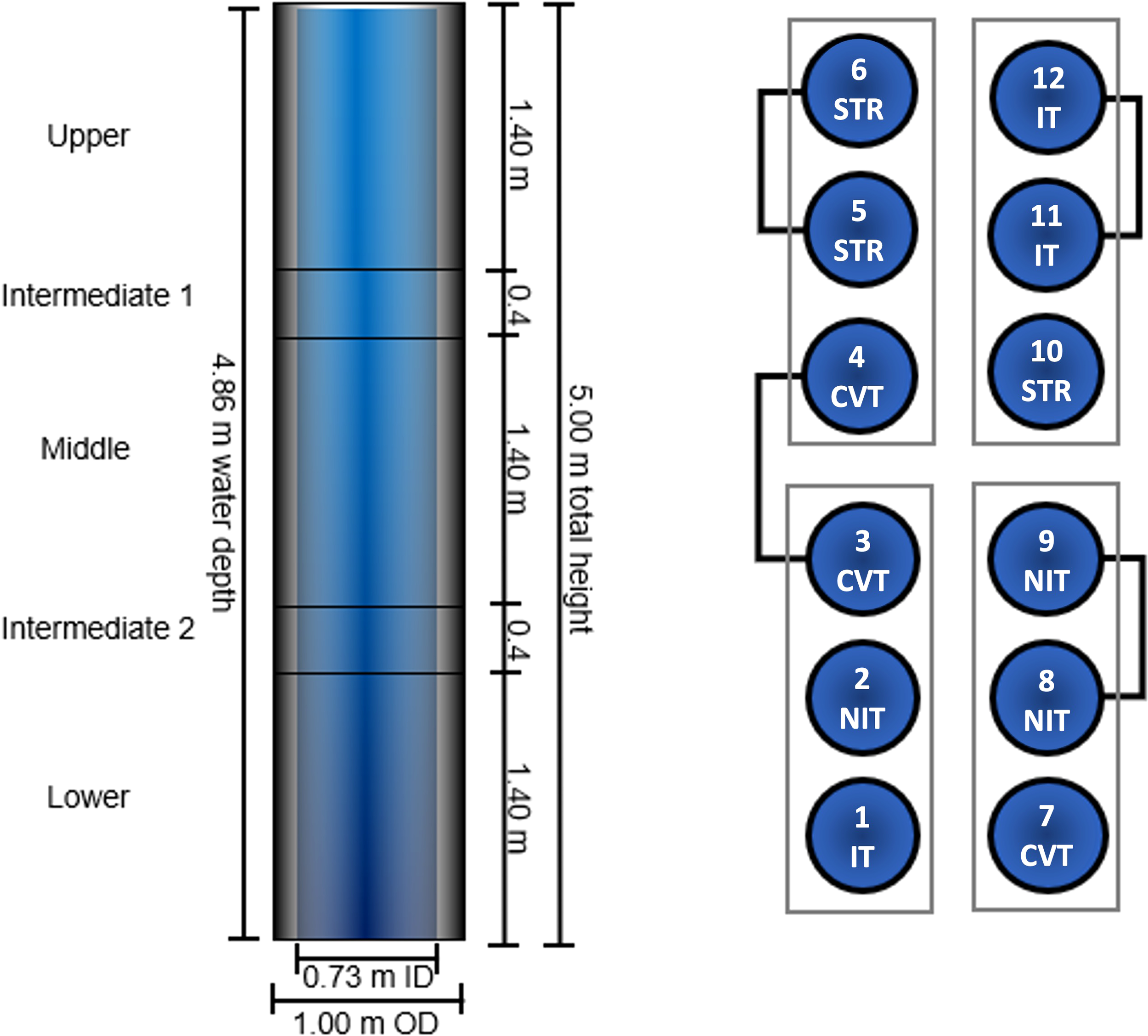
Left: vertical cross-section of a mesocosm tank. Right: schematic layout of the mesocosm facility showing the numbered mesocosms and associated temperature treatments. CVT, Convection; IT, Isothermy; NIT, Near Isothermy; STR, Stratification. Grey boxes denote refrigeration cooling units. Mesocosms linked by black lines share coolant systems. Not to scale.
The lamps above each mesocosm (LightDNA-8, Valoya Oy, Helsinki, Finland) emulate the spectra (wavelengths 380 nm to 780 nm) and intensity of the sun at every hour using a global simulation module. On top of each mesocosm, an upper refrigeration unit allows control of air temperature down to values as cold as -20°C.
2.2 Experimental set-up
Due to ice cover, water was drawn in through the offshore valve system and sampled onshore via an Aanderaa SeaGuard sonde to inform the mesocosm temperature configuration. Mirroring the average water temperature measured at the inlet, each mesocosm had a mean average temperature of 5°C across all temperature sections in the column. The temperature range was kept similar to the in-situ temperatures the phytoplankton community would experience in the natural environment as a change in temperature could alter metabolic processes, photosynthetic and/or respiration rates (Staehr and Sand-Jensen, 2006). Furthermore, even a small temperature change can significantly impact the viscosity of the water with implications for motility and sinking of phytoplankton (Margalef, 1997). The overhead refrigeration units were set to 3°C, concurrent with mean diurnal air temperature outside during the sample period.
The mesocosms were filled with offshore water via a pumped inlet situated ~800 m offshore, comprised of 50:50 water from 2-m and 8-m depth. The water was filtered through a 50-µm filter to remove any potential zooplankton grazers. Once filled, the inlet valve remained open for 10 minutes to allow any surface debris inside the tanks to be removed via the overflow pipe. The mesocosms were filled in parallel on April 24th, 2018. It took a total of six hours to fill all twelve mesocosms. The experiment ran for a total of 11 days (day 0 – 10, respectively) until 4th May 2018.
After filling, temperatures in the three sections of each mesocosm were set to specific values, so as to produce four different temperature treatments that were set in order to produce mixing regimes similar to the four natural mixing regimes identified in the introduction (and defined in Table 1). Each of the four temperature treatments were replicated three times across the twelve mesocosms:
Table 1
| Regime | Upper T (°C) | Middle T (°C) | Lower T (°C) | ΔT (°C) | Mean T (°C) |
|---|---|---|---|---|---|
| Convection (CVT) | -10 | 5 | 25 | +35 | 5 |
| Isothermy (IT) | 5 | 5 | 5 | 0 | 5 |
| Near Isothermy (NIT) | 6 | 5 | 4 | +2 | 5 |
| Stratification (STR) | 7 | 5 | 3 | +4 | 5 |
Summary of the temperature set-ups for each of the four temperature treatments.
Upper corresponds to depth 0 m to 1.6 m; middle from 1.6 m to 3.4 m; lower from 3.4 m to 5 m.
-
Convection (CVT), meant to simulate the convective mixing regime – an inverted temperature profile set to produce an unstable water column with strong convective mixing. Thus, the upper mesocosm compressor temperature was set to constant cooling in an attempt to reach an unobtainable temperature of -10°C; the middle section to 5°C; and, the lower section heater set at constant heating in an attempt to reach the unobtainable temperature of 25°C. The intention was to create energetic, ongoing overturns consistent with a higher level of turbulence.
-
Isothermy (IT), equivalent to the transitional mixing regime – a homogenous water column was maintained by setting all sections to 5°C. The intention was to create a water column with minimal temperature and density differences along the depth, resulting in homogenous, low-intensity mixing.
-
Near Isothermy (NIT), equivalent to the linearly-stratified mixing regime – The upper section had a temperature of 6°C, reduced to 5°C in the middle section, with a lower column temperature of 4°C. The intention was to create a stable yet gentle temperature gradient.
-
Stratification (STR), simulates the stratified mixing regime – a replicate of the temperature profile for the upper water column adjacent to the intake. The upper column temperature was set to 7°C, reducing to 5°C in the middle section, and then to 3°C in the lower portion. The intention was to produce a stably stratified water column with a recognizable thermocline.
The regime allocated to each mesocosm was randomized as was the daily sampling order; sampling was performed following the monitoring scheme detailed in Sections 2.3 - 2.5. The four different temperature treatments were distributed across the twelve tanks as per Figure 1.
2.3 Physical measurements
2.3.1 Stratification
A SonTek CastAway conductivity, temperature and depth sensor (CTD) was used, free-falling at a rate of 1 m/s while recording temperature, conductivity and pressure at 5 Hz. The raw data were then depth-averaged, providing readings every 30-cm depth. From these data, profiles of density were computed using the TEOS-10 toolbox with the Baltic Sea equation of state; the buoyancy frequency N was calculated from these profiles as where g is gravitational constant, and is the mean density of the profile.
2.3.2 Turbulence and mixing
Turbulent microstructure profiles were obtained using a PME Self-Contained Autonomous Microstructure Profiler (SCAMP). The SCAMP is a high-resolution CTD sensor that sinks at a constant rate of 10 cm/s through the water column while sampling at 100 Hz, enabling the measurement of microscale temperature and salinity variations. In open water, SCAMP uses a Perspex drag plate to maintain an optimum 10 cm/s decent rate. Due to the narrow diameter of the mesocosms, however, this drag plate was removed to avoid wall effects between the SCAMP and mesocosm walls. Thus, lead masses and buoyant foam rings were added accordingly to maintain the desired descent speed. Prior to the start of the experiment, a series of trial-and-error runs were carried out in a well-mixed mesocosm to ensure that SCAMP was sinking at 10 cm/s.
SCAMP profiling took place over three days from 2 May 2018 (Experiment Day T8) to 4 May 2018 (Experiment Day T10) inclusive, toward the end of the 11-day experiment. Because of the size of the instrument, profiling could not cover depths shallower than 0.5 m and deeper than 4.5 m. A total of 92 successful profiles were obtained across the twelve tanks with a median of 8 profiles per tank. Profiles were conducted at least one hour apart in each tank to permit the re-stabilization of the temperature profile should it have been disrupted during the descent and recovery of the SCAMP.
The calculation of the dissipation rate of turbulent kinetic energy (ε) via microscale variations in temperature and salinity relies on the application of the Batchelor Spectrum; a theoretical universal spectrum of one-dimensional temperature gradient fluctuations (Batchelor, 1959). Effectively, it is possible to quantify turbulence within a water column by fitting the Batchelor Spectrum to the observed temperature gradient spectrum. The application of a Batchelor Spectrum fit to high-resolution profiles allows an estimation of ε to be obtained from a temperature gradient spectrum alone.
Following the methodology of Simoncelli et al. (2018), profiles were denoised and filtered before being trimmed to remove poor-quality data at the start and end. After applying a depth offset between the SCAMP pressure sensor and the CTD sensors, each profile was segmented as per Chen et al. (2002); given the SCAMP sinking velocity of 0.1 m/s ( ± 0.05 m/s) and a sampling rate of 1000 scans/m, each profile was divided into segmentation bins of 256 (28) samples or approximately 25 cm.
First, we converted the spectra from frequency space to wavenumber space using the fall speed measured by the pressure sensor to establish the power spectral density (PSD) curve of each segment. Integrating under this PSD curve generated values for the temperature variance dissipation (χT) for each segment. The observed temperature gradient spectra are then fitted to the Batchelor Spectrum (Batchelor, 1959):
where q = universal constant (in this case, 3.4); χT = temperature variance dissipation rate (°C2/s); kB = Batchelor wavenumber (rads/s); κT = thermal diffusivity (m2/s); and, f(α) = the non-dimensional shape of the spectrum. The validity of the fit between the observed spectral fit and the Batchelor Spectrum can be quantified via the Maximum Likelihood Estimation (MLE) approach as described by Ruddick et al. (2000), allowing poor fits to be rejected.
The vertical eddy diffusivity KT (a measure of mixing) was computed for each profile with the relation from Osborn and Cox (1972):
where is the vertical gradient of the bin-averaged temperature profile. From the dissipation rate of turbulent kinetic energy (ε), the Ozmidov scale, which is representative of the turbulent eddy length scales in each tank, was computed as .
The Péclet number ( ) is a ratio between the time scales of turbulent mixing and vertical velocity (τw = LO/w; sinking/floating), where w is the vertical velocity of the cell. Pe > 1 indicates that vertical velocities exceed the rate of turbulent mixing, whereas Pe< 1 indicates turbulent mixing dominates over vertical velocity and homogenous mixing is more likely (Visser et al., 2016). To compute the vertical velocity required to overcome the turbulence in each tank, the swimming velocity threshold required for a cell was computed by solving for w with Pe = 1.
2.4 Chlorophyll-a and PAR profiles
Daily profiles were taken using an Aanderaa SeaGuard sonde, manually lowered at a rate of ~10 cm/s to reduce any mixing potential. The sonde recorded chlorophyll-a (µg/l), as well as conductivity (mS/cm), temperature (°C), pressure (kPa), dissolved oxygen concentration (µM), turbidity (FTU), and photosynthetically active radiation (PAR) The sensors on the SeaGuard are upward-pointing, allowing coverage of the water-column length within each mesocosm down to 4.5m.
The depth-normalized, integrated total chlorophyll-a (chl-a) for each mesocosm profile was calculated using the trapezoidal method whereby the integration is approximated over an interval by splitting the area into basic trapezoids.
2.5 Nutrients
Using extraction taps at different depths along each mesocosm, water samples were taken at 0.55 m, 2.3 m and 4.0 m depths, drawn into 100 ml clear PET bottles and refrigerated at 4°C until analysis later that day. Phosphate (PO43-), nitrite (NO2-), combined nitrite and nitrate (NO2-+NO3-) and ammonium (NH4+) were analyzed using a QuAAtro Autoanalyzer able to measure concentrations to a concentration limit of 0.5 µg/L. Sampling for nutrients was carried out concurrently with the extraction of biological samples.
2.6 Primary productivity
Primary productivity was measured using the 14C -CO2 technique detailed by Gargas (1975). Water samples from 0.10 m, 0.55 m and 2.30 m were drawn into two 20 ml glass scintillation vials during the morning sampling regime, obtained before 10:00am at the same time each day to ensure they were subjected to the same light intensity. 20 μl of NaH14CO3 was added to each vial. The vials were then attached to a string via rubber bands and suspended in the center of each mesocosm at their respective sample depths in duplicate pairs. The incubation was performed at midday over a period of 2 hours to be as close as possible to the midpoint of 10:00 and 14:00. Values for temperature, salinity and pH at each corresponding depth were measured using an EXO3 water-quality sonde to determine FG, the Gargas F-factor required. In addition, a control dark sample was taken at each sample depth in each mesocosm. Control vials were wrapped in foil to shield the contents from light and then placed in a water bath for two hours at 4.5°C ± 0.7°C.
20 ml of seawater was passed through a 0.2 µm filter into a small 30ml beaker. 20 µl of stock 14C-labelled sodium bicarbonate (NaH14CO3; specific activity = 0.1 mCi/mmol or 100 mCi/ml) was added to each 20 ml to attain an activity of ~1.14 mCi. The sample was shaken before extracting 100, 200, 300 and 500 µl in triplicate, adding each to individual scintillation vials containing 5 ml of filtered seawater, followed by 15 ml of Optiphase HiSafe 3 scintillation cocktail. Disintegrations per minutes (DPM) for each standard was recorded to generate a linear calibration curve. This calibration curve was used to linearly relate DPM to volume of NaH14CO3 and thus calculate the DPM reading for 1 ml of NaH14CO3 stock solution in filtered seawater. The activity of the stock solution was adjusted to account for difference in the availability of 14C in the seawater used in the experiment:
where Dstock = DPMs/ml in the original stock of NaH14CO3; Dsw = DPM/ml of the filtered seawater; Vsw = volume of filter seawater in ml (in this case, 30 ml); and, Vstock = volume of NaH14CO3 added in ml (in this case, 0.02 ml).
After two hours, vial strings were retrieved from the mesocosms. 5.0 ml was then removed from each vial via a pipette. The remaining 15 ml content was disposed of and the extracted 5 ml placed into its original incubation vial. 200 µl of formalin was then added to each vial and mixed to cease all biological activity. 150 μl 6M hydrochloric acid (HCl) was then added to each vial before subjecting the samples to bubbling for 30 minutes. 15 ml of Optiphase HiSafe 3 scintillation cocktail was then added to each sample and mixed thoroughly. Any samples exhibiting two-phase separation were mixed with additional scintillation cocktail until homogeneity was reached. Samples were placed in a Tri-Carb 2910TR Perkin Elmer liquid scintillation analyzer and the DPM reading recorded.
Primary productivity was then calculated using:
where P = rate of primary productivity (µmol C/hour/l); Dnet = measured DPM of the sample minus measured DPM in the respective dark control sample; Dtotal = measured DPM of the stock solution for the volume added to the sample; Vinc = total incubation volume in ml (in this case, 20 ml); Vsample = volume of the sample extracted for analysis in ml (in this case, 5 ml); FG = Gargas F-factor to account for the total CO2 in the sample as a result of the carbonate alkalinity, temperature, salinity and pH (obtained from Table 5.1 in Gargas (1975)); FU = a correction factor to account for the slower uptake of 14C compared to 12C equal to 1.05; FR = a correction factor to account for C loss due to respiration equal to 1.06; tinc = total incubation time in hours.
2.7 Particle identification and counts
Samples were taken at the surface and 4.0 m depth (via a draw-off tap valve on the mesocosm tanks), with ~275 ml of sample drawn into an opaque brown, wide-necked, LDPE bottle and Lugol’s fixative solution (laboratory-made as per Throndsen (1978)) added equivalent to 2% volume. The samples were stored in the dark and refrigerated at 4°C for approximately six months prior to analysis. Sampling occurred on days 0, 1, 3, 6 and 8 of the experiment.
Enumeration was carried out via a Yokogawa Fluid Imaging Inc. Flow Cytometer and Microscope (FlowCAM) system. The biomass particulate in the samples was allowed to settle in its original container before gently extracting the lower portion of the sample via a tube attached to a 100-ml syringe. The volume of excess sample not analyzed was quantified in a 250-ml measuring cylinder while the graduated syringe measured the supernatant. The ratio between the total volume of sample (excess [VE] + supernatant [VS]) to supernatant was used to calculate the dilution factor (FD) and input into the FlowCAM software to permit bulk cells per volume calculations using FD = (VS+VE)/VS. Approximately 50 ml of extracted sample was then sieved through a 100-µm filter to remove any particles that could block the FlowCAM flow cell or associated piping. Any particles/cells/detritus remaining on the filter were washed back into the sample bottle using Milli-Q water. Out of the 50 ml of filtrate, ~30 ml of fluid was passed through the FlowCAM. The flow rate was adjusted to an optimum of ~1 ml/min to balance data quality (i.e., lens focus) and time taken to process a sample. The FlowCAM used the 10x objective suitable for cells between 8 µm to 100 µm. The imaging camera was set to a frame rate of 20 frames/s in order to obtain an optimum particles/image as close to 1 as possible.
A total of 462,156 images were taken by the FlowCAM. Using the VisualSpreadsheet 4 software, easily identifiable particles were manually sorted and placed into ID reference libraries until the recommended minimum of 60 images was reached for each taxonomic group. Images were sorted accordingly until at least 90% of the images had been catalogued; a mean of 93% of each sample was catalogued. The remaining 10% were comprised of: cells too small to have sufficient resolution to catalogue, out-of-focus cells, and/or miscellaneous images that did not easily fit into the main categories.
For cells<14 µm in length, the FlowCAM resolution was insufficient to identify the genus/species; thus, these were cross-referenced with long-term periodic monitoring data from the Umeå Marine Sciences Centre over the same period to ascertain potential candidates. Certain species and taxa (Mesodinium rubrum, oligotrichids, small flagellates, Gymnodiniales) were observed to participate in the formation of conglomerates consisting of multiple cells and different taxa within the same image; in this instance, these were sorted separately and enumerated accordingly. For enumeration purposes, 271 images of flagellate conglomerates from randomly selected and samples across all four turbulence regimes were manually counted; images contained a mean of 4.0 flagellate cells (STDEV = 3.3). This value was then used as a multiplier for the number of conglomerate images. Cell abundance changes due to Lugol’s preservation have been adjusted in accordance with Zarauz and Irigoien (2008).
From the cell counts for each mesocosm on a given sampling occasion, we calculated the location index as cell counts at 0.1 m depth, divided by the sum of cell counts at 0.1 m and 4 m. This index was calculated for each taxonomic unit we identified. It gives an indication of the preferential location of a given taxonomic unit between the surface and the bottom of the mesocosm. It is of note, though, that given that only one specific depth at the surface and at the bottom were sampled, results do not necessarily reflect the percentage of cells at the surface vs the bottom.
2.8 Statistical analysis
Generalized additive models (GAMs) were tested to ascertain the link between the parameters measured (temperature, density, buoyancy, turbulent dissipation rate, eddy diffusivity, Ozmidov scale, vertical velocity threshold, PAR profile, nutrient concentrations, chlorophyll-a, and location index), and depth, temperature treatment and sampling day —where appropriate — as independent factors. Potential effects of mesocosm identity were included as random effects. Alternative models were compared using the Akaike Information Criterion (AIC). The best models selected according to this procedure were used to generate predicted mean effects within each treatment level and confidence intervals around the predictions. All statistical analyses were conducted using the R software (version 4.2.2) and the mgcv package (version 1.8-41). The code is available as supplementary material (link).
3 Results
3.1 Physical properties of the water column differ between treatments
Varying the heating treatment between each mesocosm elicited different temperatures profiles that fit, to a large extent, the natural profiles they are expected to mimic (Figure 2A). The stratified (STR) treatment shows a clear two-layer system with a mid-depth thermocline dividing a warmer (7°C) upper layer and a cooler (3°C) bottom layer. Near-isothermal mesocosms (NIT) exhibit a stable water column with surface temperatures of ~ 6.0°C, steadily decreasing to ~3.5°C at depth. The convection (CVT) and isothermal (IT) treatments exhibit well-mixed profiles with constant 5°C temperatures along the depth.
Figure 2
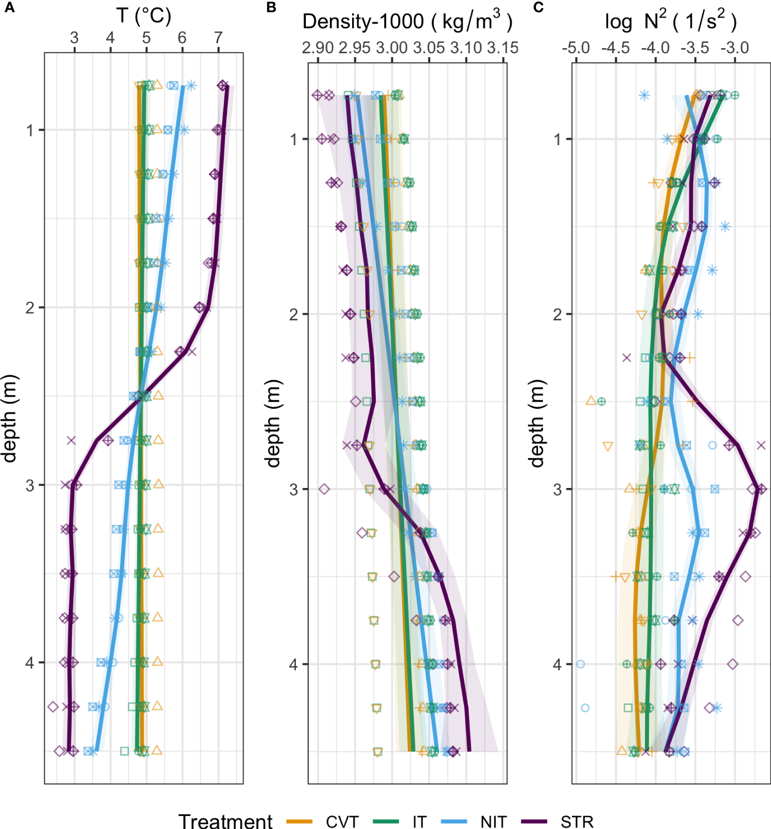
Mean physical SCAMP profiles for each temperature treatment (CVT is convection; IT, isothermy; NIT, near isothermy; and STR, stratification). (A) Temperature; (B) Density; (C) Buoyancy frequency (N2); Solid lines (—) show the values predicted by the best GAM model, as selected using the AIC criterion; the shaded ribbon around the line represents the 95% confidence interval around the prediction. Points represent the data measured, averaged within bins of widths of approximately 25 cm and over all profiling events. The 12 different shape symbols represent the 12 mesocosms.
These treatment differences are echoed in the density profiles (Figure 2B). Changes in density with depth are very modest. Still, the STR treatment shows a clear pycnocline. The NIT treatment shows a continuous increase in density with depth, without any visible pycnocline. Finally, the CVT and IT treatments show even weaker gradients in density. The patterns in buoyancy frequency (Figure 2C) reflect the density profiles.
3.2 Turbulence and mixing reflect the different temperature treatments
The turbulent eddy diffusivity (KT; a measure of vertical mixing) values in all treatments were in the range typically experienced in the open ocean (Figure 3A). As expected, the mixing in the CVT treatment was generally the highest, followed by the IT treatment, then the NIT treatment. Mixing in the STR treatment followed a different pattern than the others – weak mixing was generated above the thermocline, but it appears that below the thermocline the temperature setup induced more mixing than at the surface.
Figure 3
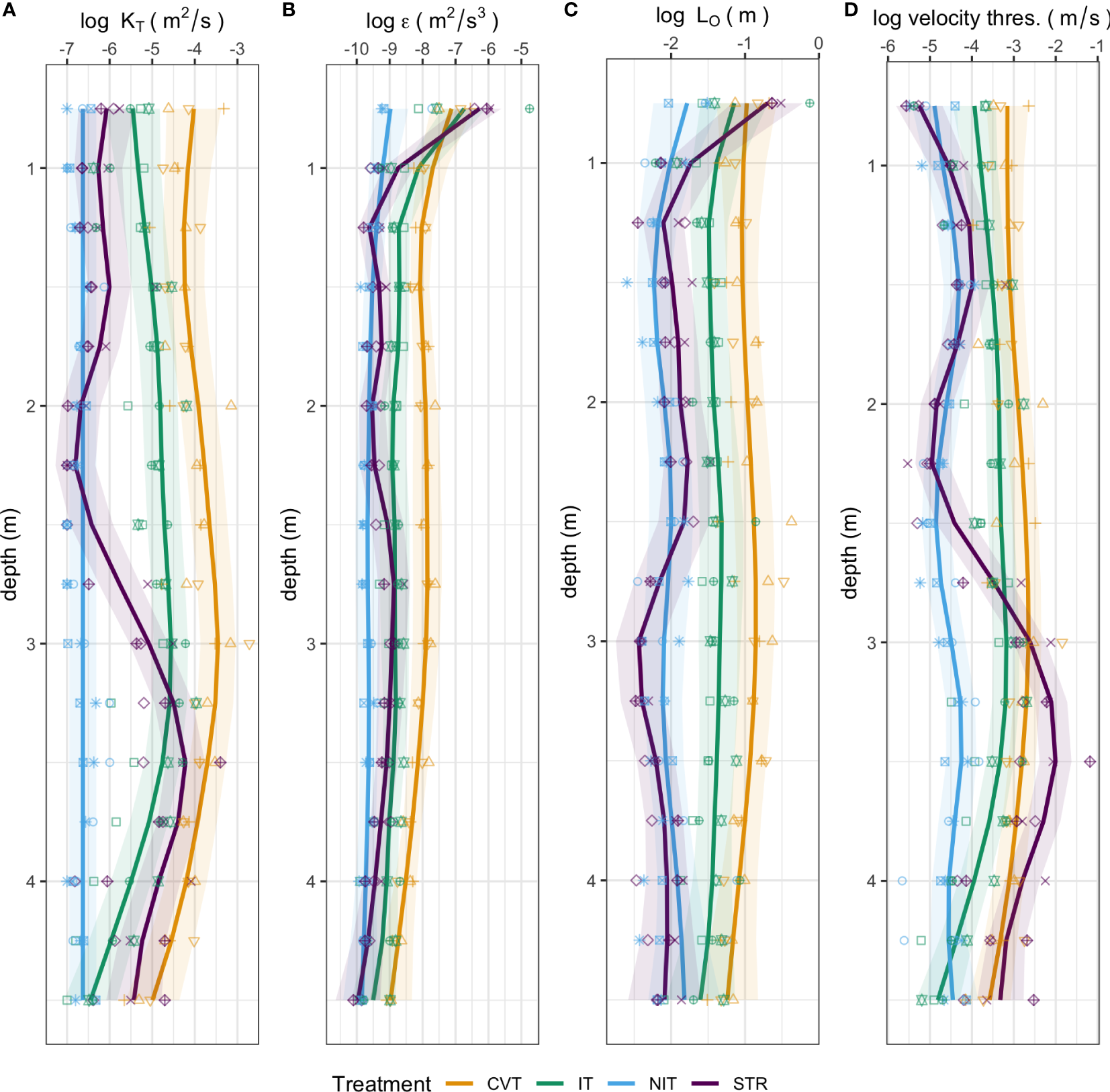
Mean calculated profiles of turbulence-related parameters for each temperature treatment (CVT is convection; IT, isothermy; NIT, near isothermy; and STR, stratification). (A) Turbulent eddy diffusivity (KT); (B) Turbulent dissipation rate (ε); (C) Ozmidov length scale (LO); (D) Vertical velocity threshold; Solid lines (—) show the values predicted by the best GAM model, as selected using the AIC criterion; the shaded ribbon around the line represents the 95% confidence interval around the prediction. Points represent the data measured, averaged within bins of widths of approximately 25 cm and over all profiling events. The 12 different shape symbols represent the 12 mesocosms.
Profiles of turbulent dissipation rates (ε) are clearly distinct between treatments (Figure 3B). Under convective mixing (CVT), dissipation rates are nearly constant with depth, at high values between 10-8-10-7 m2/s3. Only at the lowest depths do we see a decrease to values around 10-9 m2/s3, values which are typical of deeper pelagic waters. The IT treatment shows a very similar pattern, but with values that are one order of magnitude lower. The NIT treatment shows the lowest dissipation rates overall, with values between 10-10-10-9 m2/s3. More interestingly, the stratified treatment (STR) also reached similarly low values at some depths; however, it also reaches the highest dissipation rates (around 10-6 m2/s3) in the very top layer.
Profiles for the Ozmidov length scale (LO) are very similar to those of ε (Figure 3C). Typical length scales are ~10 cm in the CVT treatment, slightly shorter in the IT treatment, ~1 cm in the NIT treatment, and vary from 10 cm at the very top layer to 1 cm at below depths for the STR treatment.
Vertical velocity thresholds show remarkable consistency in the CVT and NIT treatments, with respective typical velocities on the order of 10-3 m/s and 10-5 m/s (Figure 3D). Typical values are intermediate in the isothermal treatment (around 10-4 m/s). Interestingly, they fall by an order of magnitude near the bottom of the mesocosms. As for most of the other physical parameters, the stratified treatment yields the most uneven profiles, with thresholds that are lowest at the very top and near the thermocline depth, and highest below the thermocline.
3.3 Chlorophyll-a profiles and primary productivity diverge between treatments
All treatments started with similar depth profiles on day 0 (measured just a few hours after the onset of the different temperature treatments). However, the profiles developed differently as the experiment progressed (Figure 4). Under convection, chl-a showed a slight increase near the top of the water column (above ~2 m) while concentrations remained the same at lower depths, around ~ 0.8 µg/l. After day 6, chl-a concentrations at the top returned back to their initial concentrations. IT mesocosms showed similar patterns as for CVT with one recognizable difference: starting from day 3, chl-a concentrations increased at 4.5 m depth (and most probably at lower depths as well). A similar increase in chl-a concentrations at depth can be seen in the NIT treatment, starting from day 2. This treatment shows also a markedly higher increase at the top layer than the CVT and IT treatments, with maximum mean concentrations recorded on day 5, followed by an ebbing in concentrations. Chl-a profile development in the STR treatment showed the most unique properties, with first a large increase in concentrations at an intermediate depth (between 1-2 m) on day 2 and 3, overtaken by an increase at top layers. Similar to the other treatments, any increase in chl-a concentration reverted to original values by the end of the experimental period, so that profiles at the end (day 10) are very similar to the profiles at the beginning (day 0).
Figure 4
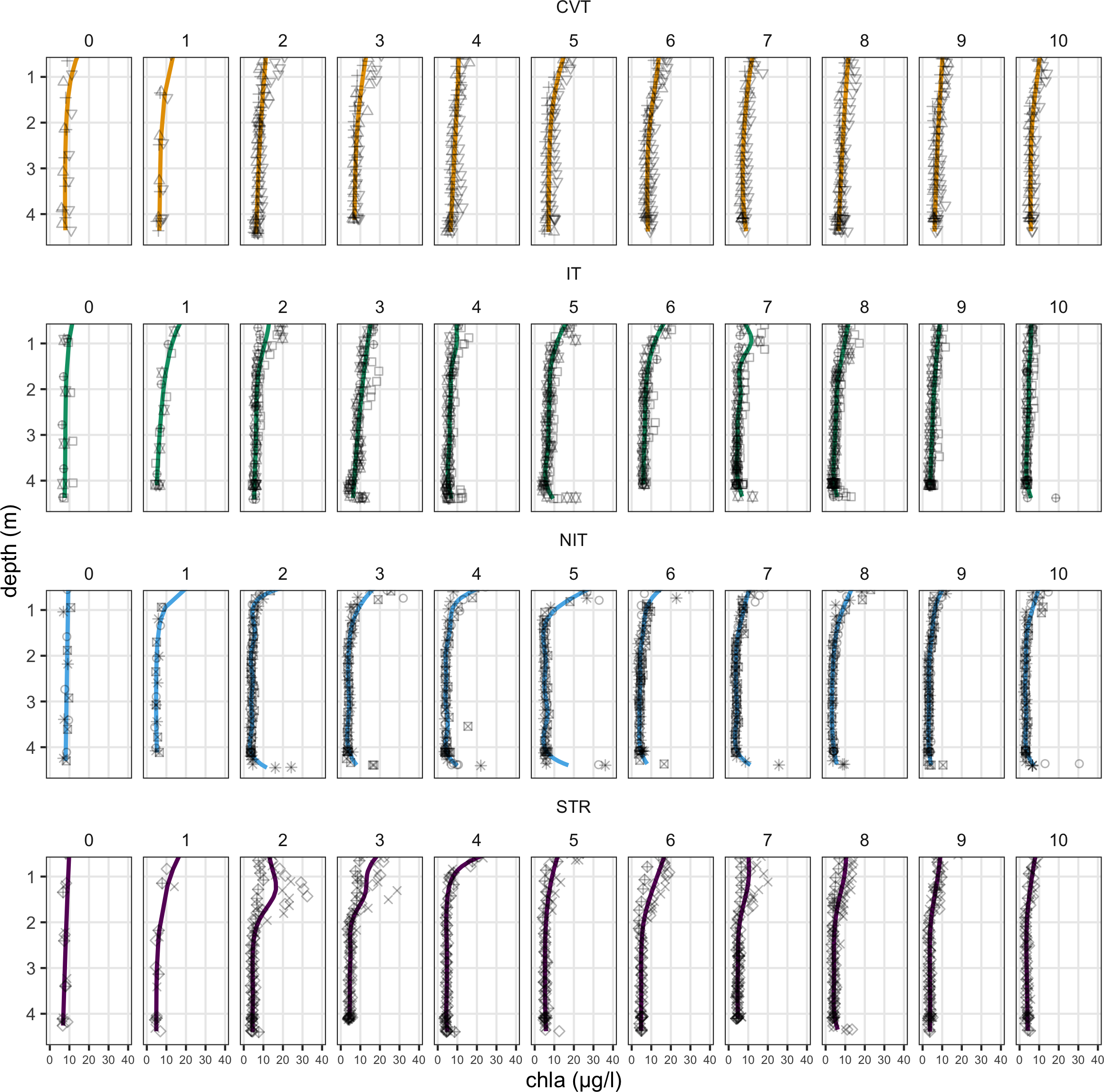
Chlorophyll-a profiles from day 0 to day 10 for the four temperature treatments (CVT is convection; IT, isothermy; NIT, near isothermy; and STR, stratification). Solid lines (—) show the values predicted by the best GAM model, selected using the AIC criterion; points represent the data measured, averaged within bins of widths of approximately 25 cm and over all profiling events. The 12 different shape symbols represent the 12 mesocosms.
When integrated over the whole water-column depth, mean chl-a concentrations did not differ significantly between treatment levels (Figure 5). All showed a slight increase from initial concentrations around 9 µg/l on day 0, along experimental time, before a clear decrease in concentration, reaching down to concentrations around 5 µg/l on day 10. The STR treatment diverged from the main observed trend though, reaching maximum concentrations later in the experiment (around day 5 instead of day 3) and decreasing to lowest values that still remained well above 6 µg/l.
Figure 5
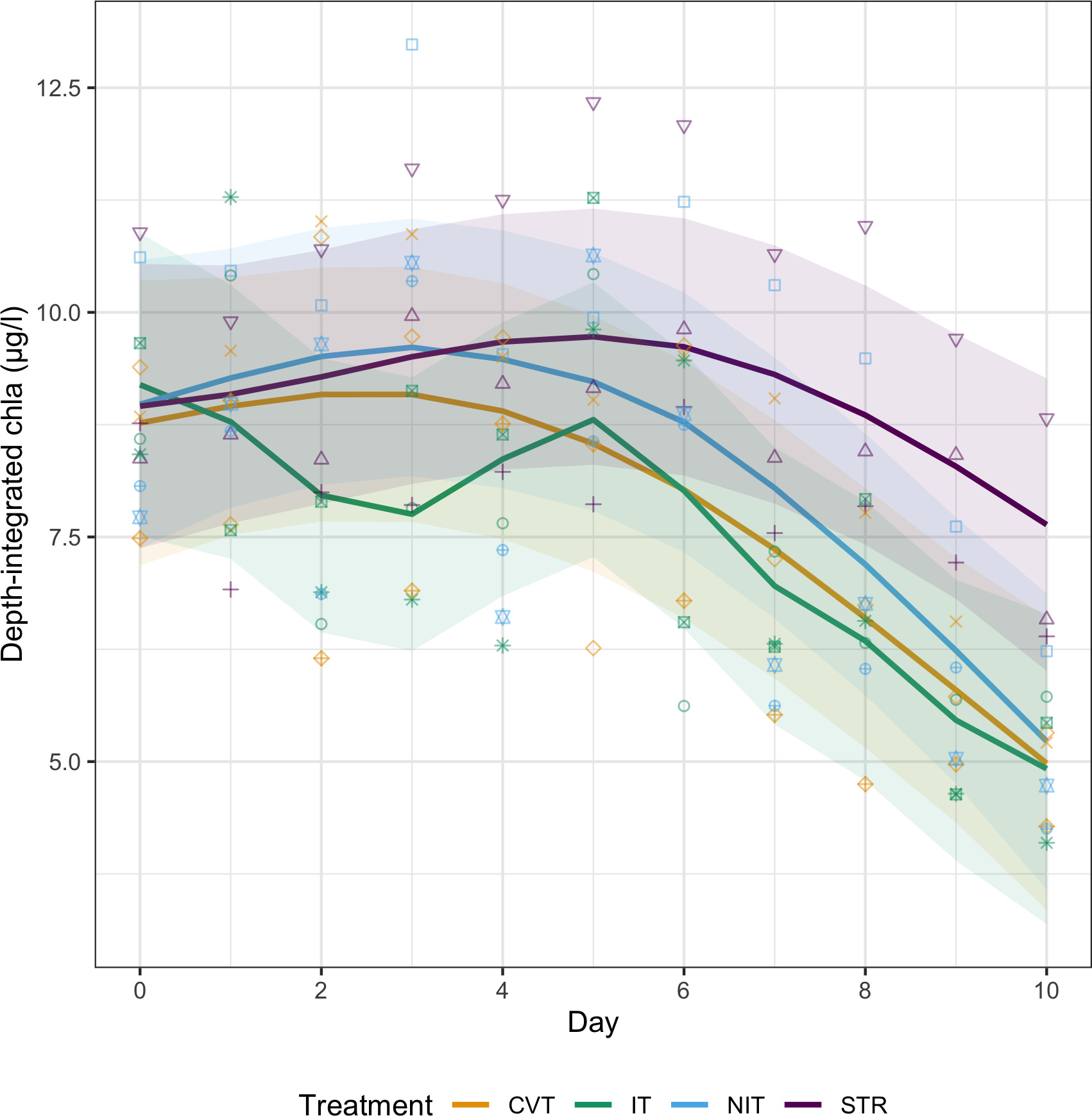
Depth-integrated chlorophyll-a concentrations from day 0 to day 10 for the four temperature treatments (CVT is convection; IT, isothermy; NIT, near isothermy; and STR, stratification). Solid lines (—) show the values predicted by the best GAM model, selected using the AIC criterion; points represent the data measured. The 12 different shape symbols represent the 12 mesocosms.
Measured at three different depths (at the surface, a short distance below the surface, and near the depth of the thermocline of the stratified treatment), primary productivity showed a slight increase at the two shallowest depths in the CVT and IT treatments between Day 0 and 1 (Figure 6). They then kept at almost constant values for the remainder of the experiment. The STR and NIT treatments showed a remarkable increase at the surface, before steadily declining to values similar to those of the other treatments near the end of the experiment.
Figure 6
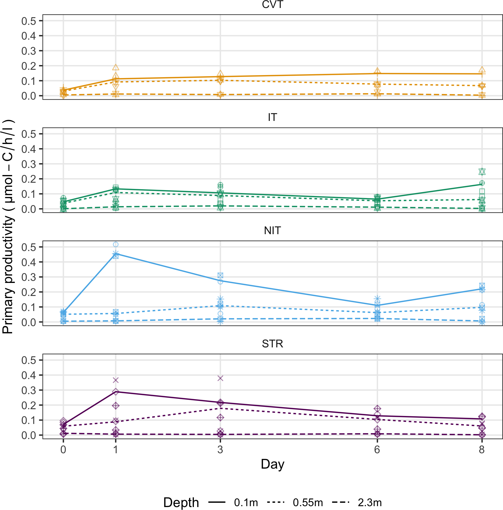
Primary productivity (µmol-C/h/l) measured at three different depths, on five occasions during the experiment for the four temperature treatments (CVT is convection; IT, isothermy; NIT, near isothermy; and STR, stratification). Lines show the values predicted by the best GAM model, selected using the AIC criterion; points represent the data measured. The 12 different shape symbols represent the 12 mesocosms.
3.4 Phytoplankton resources reflect the chl-a and primary productivity patterns
Light profiles between treatments and days are significantly different at the statistical level, but the differences are quantitatively very small, so as to be identical (Figure 7). Hence, the phytoplankton under the different treatments grew up under very similar light regimes over the whole experiment.
Figure 7
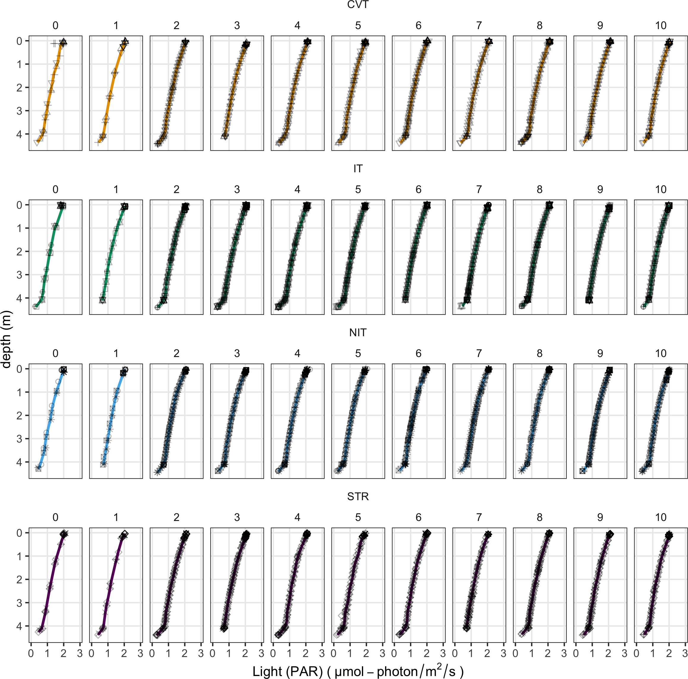
Photosynthetically active radiation profiles from day 0 to day 10 for the four temperature treatments (CVT is convection; IT, isothermy; NIT, near isothermy; and STR, stratification). Lines show the values predicted by the best GAM model, selected using the AIC criterion; points represent the data measured. The 12 different shape symbols represent the 12 mesocosms.
Contrary to light, nutrient patterns differ between treatments and along the experiment (Figure 8). Nitrate plus nitrite concentrations drastically decreased during the first days in all treatments (Day 0-3) and at all depths for all treatments. Still, the decrease was steeper at the surface than at the mid- and bottom-depths in the NIT and STR treatments, resulting in a gradient of increasing concentrations with depth. After day 3, there was an inversion in the gradient of concentration with depth in these treatments. Concentrations at the surface increase on day 8 for all treatments. Patterns in ammonium and phosphate are different from nitrate plus nitrite, but are similar to each other. They show only slight variations along time, with a small tendency to decrease at depth and increase at the surface. The surface increase is even more marked in the STR and NIT treatments.
Figure 8
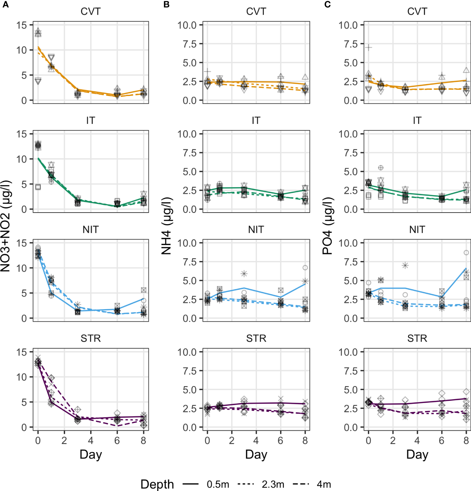
Nutrient concentrations: (A) [NO3-]+[NO2-], (B) [NH4+], and (C) [PO43-], measured at three different depths, on five occasions during the experiment for the four temperature treatments (CVT is convection; IT, isothermy; NIT, near isothermy; and STR, stratification). Lines show the values predicted by the best GAM model, selected using the AIC criterion; points represent the data measured. The 12 different shape symbols represent the 12 mesocosms.
3.5 Differences in mixing of phytoplankton species between treatments
The location index, i.e., an indication of the relative preference of a given taxa for the surface relative to the bottom (as quantified by the cell count at 0.1 m below the surface divided by the sum of cell counts at 0.1 m and 4m; Figure 9), evolved differently along the experiment for different taxa. Already from day 0, taxa diverge in their relative locations. Most taxa show location index values close to 0.5, i.e., as many cells are counted in the surface sample as in the bottom sample. However, a few taxa show location indices that span the whole range of possible values (from 0 to 1) already from day 0 (see, e.g., Thalassiosira, Melosira, Peridiniella, and Tintinnida). Generally, these taxa kept spanning the whole range of location index values on the following sampling days, without any obvious relation to the temperature treatments. Those taxa were motile (Peridiniella and Tintinnida) or nonmotile (Thalassiosira, Melosira, Pauliella). Other taxa maintained similar densities at the surface and the bottom (i.e., location index = 0.5) from the start to the end of the experiment (Centrales, pennates, Monoraphidium, and to a lesser extent, Cylindrotheca, and flagellates). For these taxa, no obvious size or taxonomical signal distinguishes them from the other taxa. Remarkably, Uroglenopsis, a motile chrysophyte, was mostly found in the surface samples even from the start of the experiment. Even more remarkable are Peridiniales, also a motile taxon, which were only found in the surface samples for all sampling days. Finally, two ciliate taxa, Oligotrichids and Mesodinium, were predominantly counted in surface samples, although they also maintained a significant presence in bottom samples, particularly on the first days.
Figure 9
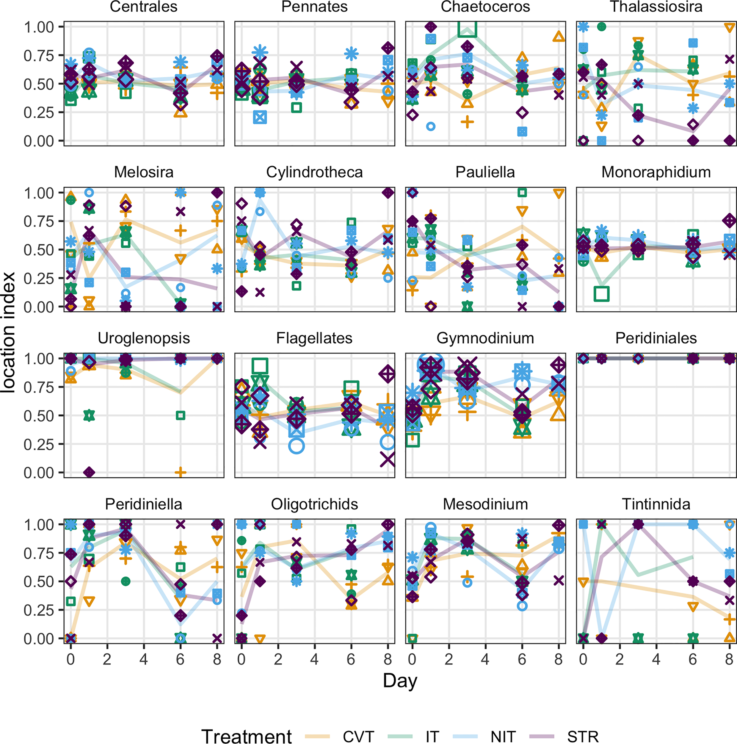
Location index (cell counts at 0.1m below the surface divided by cell counts at 0.1m+ cell counts at 4m) measured at five sampling dates (days 0, 1, 3, 6 and 8) for the phytoplankton taxonomic units identified in the mesocosms, for the four treatments (CVT is convection; IT, isothermy; NIT, near isothermy; and STR, stratification). Taxa a-g are diatoms, h is a chlorophyte, i is a chrysophyte (motile), j-m are dinoflagellates (motile) and n-p are ciliates (motile). A value of 1 indicates that all cells of the taxonomic unit were counted in the surface sample; a value of 0 means all cells were in the bottom sample; and a value of 0.5 means that as many cells were counted in the surface as in the bottom sample. Solid lines (—) show the values predicted by the best GAM model, selected using the AIC criterion; points represent the data measured. The 12 different shape symbols represent the 12 mesocosms. The size of the shapes are proportional to total counts (cell counts at 0.1m + cell counts at 4m).
4 Discussion
4.1 Convective mixing in mesocosms as a means to simulate natural regimes
Mesocosms are an established method to study climate change (Stewart et al., 2013). However, most of them suffer from shortcomings that restrict extrapolation of the experimental results (Arnott et al., 2021). In particular, the turbulent dissipation rates generated by mechanical means (grids, paddles, etc.) are generally larger than the typical range measured in natural conditions (10-10 to 10-7 m2/s3 under pelagic conditions) or produce distorted patterns of turbulence (Nerheim et al., 2002). Under pelagic conditions, turbulence patterns depend on the balance between wind-induced shear and heat forcing (Pernica et al., 2014). Typical mixing profiles are i) convectively mixed waters, where cooling of surface waters leads to their sinking and, hence, to the overturn of the upper layer of the water column (Shay and Gregg, 1986), ii) isothermal waters, where temperatures at the top and bottom of the water column are the same, leading to similar temperatures throughout the water column, iii) weakly stratified waters, where slightly warmer surface waters result in a linear gradient of decreasing temperatures with depth, and iv) stratified waters, where the balance between heat forcing and low wind stress allows for a thermocline to establish at an intermediate depth (Wells and Troy, 2022).
In our experiment, we focus on one factor, temperature-controlled buoyancy fluxes, to generate these four typical mixing profiles in indoor mesocosms. Not only did we obtain stratified waters in the stratification treatment, but we were also able to create a thinner, actively mixing layer at the top of the column, embedded within a wider mixed layer (a typical feature of stratified waters, see Franks, 2015). By cooling the top section of the mesocosms and warming their bottom section, we managed to simulate the effect of surface cooling, creating convection treatments whose dissipation rates and eddy diffusivities are typical of convective mixing (ε values between 10-9-10-7 m2/s3, and KT values below 10-3 m/s; Cannon et al., 2019). The isothermal treatment also resulted in a well-mixed column, with constant temperature and a minimal density gradient. However, as expected, the level of mixing was an order of magnitude lower than in the convection treatment. Also as anticipated, the nearly isothermal treatment showed the smallest levels of turbulence throughout the water column, as exemplified by the very low turbulent dissipation rates (ε< 10-9 m2/s3) and small Ozmidov length scales (LO ≈ 10-2 m). On the other hand, given its relatively high buoyancy frequency values (second after the stratification treatment), this is the treatment with the least mixing and exchange between layers, hence the low turbulent diffusivities (KT ≈ 2.3x10⁻⁷ m2/s). Ultimately, based on the measured physical parameters, we were able to establish temperature-controlled mesocosms that simulate the main buoyancy-controlled natural mixing regimes.
There are clearly limitations to our approach. Most of them are inherent to the mesocosm method: enclosure prevents side-water exchanges and corresponding horizontal dispersion (Wells and Troy, 2022); the vertical scale is compressed such that profiles that develop over tens to hundreds of meters in lakes and oceans are compressed within 5 meters. Moreover, because our mesocosms were set indoors, wind shear was eliminated as a source of turbulence. It is difficult currently to think of experimental designs that can generate different buoyancy-controlled mixing regimes within containers of relevant horizontal and vertical dimensions, while also allowing for different degrees of simulated wind shear indoors. Alternatively, there already exist outdoor mesocosm facilities that allow for a surprisingly large deal of control (see, e.g., the Kiel Outdoor Benthocosms, in Wahl et al., 2015). In-situ enclosures might, at first glance, appear to be an even better alternative to indoor or outdoor mesocosms, because of their ease of deployment in the field, their cost-effectiveness, and their closeness to natural conditions (Arnott et al., 2021). However, when it comes to turbulence specifically, their realism is questionable. Most of in-situ mesocosms use flexible plastic walls which, depending on the setup and context, either dampen turbulent mixing (Sanford, 1997) or enhance inside turbulence because of wave-enclosure interactions (Svensen et al., 2001). More dramatically, large perturbations can override any turbulence treatment by the experimenters. Indeed, because turbulence is directly affected by temperature and shear, it is very sensitive to unpredictable meteorological variations (Jöhnk et al., 2008). If we add as a consideration the technical difficulties of controlling the temperature of several mesocosms simultaneously at several depths in the field, we consider that convection-driven methods similar to ours are not ready to be deployed in-situ. There are however reasons to hope that technical improvements to such infrastructure could make field, convective-driven mesocosms a reality in the near-future (see, e.g., the KOSMOS mesocosms that allow for a better control of turbulence within off-shore enclosures, as in Mathesius et al., 2020). In the meantime, results from indoor mesocosms should not be dismissed, as long as rigorous measurements of the experimental conditions and coupling with existing theory are carefully conducted (Benton et al., 2007; Vijayaraj et al., 2022).
4.2 Response at the plankton level show consistent patterns and highlight resilience to changes in mixing regimes
In order to assess whether realistic physical features of different mixing regimes translated into realistic biological responses, we measured daily chl-a profiles within all the mesocosms. The profiles are typical of the corresponding simulated mixing regimes: mostly constant along the column for the convection and isothermal treatments; larger at the top in the nearly isothermal treatment (equivalent to the weak linearly stratified regime), and with a maximum chl-a layer below the surface and above the thermocline in the stratified treatment (Franks et al., 2022).
There were inherent limitations to our assessment of the phytoplankton community response to the different temperature treatments with the use of the location index: i) taxonomic resolution differed between the various taxa, and was very shallow for some of them; ii) the FlowCAM used could not measure cells below 8 µm and the water used for filling the mesocosms was prefiltered through a 50-µm filter; thus, identification was restricted to taxa between 8-50 µm; and iii) we sampled the community only once every two days, and only at two depths (10 cm below the surface and at 4 m depth). As we do not have counts along most of the depth of the water column, we cannot use the location index to link chl-a concentrations to specific taxa. Neither can we use the location index to infer the preferred location of a given taxon. For example, the presence of Peridiniales only in our surface samples does not preclude the possibility for even higher densities of this taxon at depths between 0.1 and 4 m. With these restrictions in mind, interesting and compelling conclusions can still be drawn from the location index analysis.
The most striking result is the absence of any systematic effect of treatment on the index. Apart from Uroglenopsis, a motile chrysophyte, which tended to be found more often in bottom samples in the convection and isothermal treatments, the location of the other taxa was not affected by treatments in any systematic way (statistical effects are significant in some instances, but are rather idiosyncratic). In contrast, expectations in the literature are clear: large, non-motile diatoms suffer from stratification and thrive under convection (Huisman et al., 2004; Bopp et al., 2005); the opposite is true for small, motile dinoflagellates (Villamaña et al., 2019). We can only infer indirect explanations for the absence of such patterns in our experiment:
Swimming velocities in motile species are very variable and surprisingly unrelated to size (Lisicki et al., 2019). They range between 10-6-10-4 m/s with some taxa that can reach exceptional velocities in the range of 10-3-10-2 m/s. The sinking velocities of non-motile species within the 8-50 µm size range are even lower (Pančić and Kiørboe, 2018). Given that the vertical velocity thresholds we measured in the four treatments (CVT, IT, NIT and STR) were within the same range (10-6-10-2 m/s), we conclude that turbulent eddies and buoyancy fluxes in all treatments should, if not overcome, at least interfere with the vertical movement of all species. Despite this likely disruptive effect of mixing, it is noticeable that some motile taxa, such as Peridiniales and Uroglenopsis, are able to select and maintain their position very precisely in the water column.
The location index for most species was actually observed to deviate from the 0.5 value (i.e., identical distribution between top and bottom samples) during the course of the experiment, indicating that mixing was probably not the only factor shaping their vertical distributions. Given the high densities of mixotrophic grazers (large flagellates and ciliates) in the mesocosms, we expect predation to be one of these factors. Many phytoplankton species are also capable of changing their internal density and, thus, their sinking rates. Some diatoms can even alter their buoyancy in a matter of a few seconds in response to fluid shear (Arrieta et al., 2020). Besides vertical relocation, turbulence also imparts small-scale effects on phytoplankton (e.g., decreasing growth rate, increasing nutrient uptake rates, see Peters and Marrasé, 2000). Moreover, varying light and nutrient availabilities with depth may have altered the localized growth rate of each taxon in different ways. Given the number and complexity of the potential factors involved in determining cell densities of given taxa at each depth, and given the spatial limitation of our sampling effort in this experiment, understanding the full effect of the different mixing regimes on the distribution of the various taxa is out of the scope of this experiment.
4.3 Insights for climate change effects on phytoplankton communities
Our experiment highlights several interesting points regarding the potential effects of climate change on phytoplankton community composition and production via changes in buoyancy-controlled mixing. In terms of species composition, the narrative of an increased dominance of dinoflagellates at the expense of diatoms with increased climate change should perhaps be nuanced (see, e.g., Edwards et al., 2022). Given the similar response of most taxa to the different treatments within the span of our experiment, the occurrence of such a shift may be attributed to the influence of several physiological and ecological factors, beyond mere hydrodynamical effects. Long periods of stratification may lead to nutrient depletion in the surface layer (Falkowski and Oliver, 2007). They may also reduce the inorganic C influx into the surface layer (Havskum and Hansen, 2006). Moreover, surface temperatures and light availabilities may reach higher values at the surface (Mousing et al., 2014). Hence, overall, increased stratification due to climate change may promote those species that are better at using improved light and temperature conditions at the surface in order to harness more efficiently the resources that become more limiting, such as nitrogen and inorganic carbon (Falkowski and Oliver, 2007; van de waal and Litchman, 2020).
Besides, indications of a strong top-down control of phytoplankton production, even in the absence of grazers above a size of 50 µm, suggest that understanding the impact of increased stratification due to climate change requires the consideration of predator-prey interactions, as advocated in Behrenfeld and Boss (2014).
Furthermore, significant settling seemed to take place only in the treatments with the lowest mixing rates at the bottom of the water column. Hence, climate change is likely to increase the sinking of phytoplankton particles below the upper layers only if there is a concomitant decrease in the mixing of the lower layers.
Even if our experiment does not bring firm conclusions on the role of mixing regimes for phytoplankton production and community composition, results yield a valuable set of realistic physical and physiological properties that clearly ascribe the differences observed between controlled temperature and mixing treatments to the same factors influencing natural mixing regimes. As such, we think that buoyancy-controlled mixing in mesocosms coupled, if possible, with devices to generate surface shear similar to wind shear, represents the most appropriate experimental approach to explore the mechanistic links between climate changes factors and the associated phytoplankton response.
4.4 Contribution of experimental convection mixing to plankton theory development
Turbulence plays a role in almost all plankton ecology theories, sometime major, other times minor, sometimes explicit, other times implicit (see, e.g., Peters and Marrasé, 2000; Huisman et al., 2002; Roy and Chattopadhyay, 2007). But in absence of experimental designs that reproduce realistic turbulence, convincing tests of these hypotheses are still pending (Franks, 2015). We will show in this last section how our convection-based mesocosm approach, which allowed us to create contrasted mixing regimes makes a significant step forward in this direction. Although we did not plan our first implementation of buoyancy-driven mixing mesocosms with the explicit objective to test any given plankton theory, useful inferences can be drawn from the comparison of the four treatments. In particular, the mean temperature, turbulent intensities, and experiment duration for the four treatments were similar to the conditions during the transition sequence in mixing regimes (chronologically, pelagic waters go from convection to stratification regimes via the transitional/isothermal and linearly-stratified regimes) that occur in the spring in the Bothnian sea (Pärn et al., 2022). Most theories that explain the onset of spring blooms focus on this transition period. However, these theories highlight different mechanisms and make different predictions regarding the timing of phytoplankton growth and increases in densities (Behrenfeld and Boss, 2014). Chronologically the first, Sverdrup’s critical depth hypothesis (Sverdrup 1954) times the start of the spring bloom to the onset of the stratified regime: as the thermocline decreases to reach the light compensation depth, the light-limited phytoplankton is trapped in the illuminated, mixed surface layer, where it finds favorable conditions for an increased primary productivity, transitioning to nutrient limitation. Indeed, in our experiment, Larger total chl-a concentrations can indeed be observed in the stratified treatment relative to the other treatments, with a peak in concentration just above the thermocline, as predicted by the hypothesis. However, this peak rapidly erodes, and almost disappears after day 7. Moreover, we see no evidence for light limitation in any of the treatments. Rather, the decline in NO3- and NO2- concentrations, but not in PO43-, indicates nitrogen limitation in all treatments, irrespective of the mixing regime. Hence, we conclude that our experiment only offers partial support for the critical depth hypothesis.
The critical turbulence hypothesis singles out the decrease in turbulence intensity that takes place at the end of the convective mixing period, i.e., the transitional regime, as the cause for the onset of a bloom in the layers closest to the surface. In the context of our experiment, this means that we should expect an increase in chl-a and in primary productivity at the top of the mesocosms in the isothermal treatment, in comparison to the convective mixing regime. No such increase was observed, however. Moreover, in this hypothesis, as in the critical depth hypothesis, light plays a major role, and thus, a shift in limitation from light in the convective mixing regime, to nutrients in the isothermal regime is expected. No such shift was observed, yielding no support for this hypothesis.
A more recent and complex hypothesis, the disturbance-recovery hypothesis (Behrenfeld and Boss, 2014), sets the initiation of the growth phase of the bloom much earlier, in early winter, when the transition from near isothermal to convective conditions takes place. The mechanism postulated is the dilution in grazers’ density due to their entrainment toward lower depths thus freeing the phytoplankton from predation losses. However, because the phytoplankton is also convectively dispersed over a deeper water column, their increase in growth rate does not translate into accumulated biomass until convective mixing stops and stratification consolidates again. In the context of our experiment, we should expect a surge in instantaneous growth rate, when comparing the isothermal treatment to the convection treatment. No increase in primary productivity was observed between the two treatments in our experiment. We thus have very little direct support to offer for the disturbance-recovery hypothesis. We do have some indirect evidence though that supports one tenet of the hypothesis; namely, the importance of phytoplankton growth control by grazers. In our mesocosms, as is the case in Northern Baltic waters, large mixotrophs, such as Mesodinium sp., are a major component of the phytoplankton community. Overall, there was a very modest increase in total chl-a concentrations in all mesocosms, followed by a marked decrease to values below starting concentrations. If interpreted as the result of a strong top-down control of the phytoplankton growth by mixotrophic grazers, this is an indication for a significant role of grazing in the growth of phytoplankton. Such a top-down effect is compatible with a possible role of decreased nitrate concentrations in the second half of the experiment, that may have curtailed the ability of the phytoplankton to respond to the grazing pressure of the mixotrophs and heterotrophic protists.
We conclude from this exercise that no hypothesis was fully supported by our data. Perhaps the reason lies in a hidden assumption that is shared by the three hypotheses, namely that the vertical distribution of the plankton is almost entirely shaped by the mixing regime, such that they expect the phytoplankton to be concentrated within the top layer under stratification, and to be distributed over the whole water column under convection. However, the location index in our experiment suggests that plankton distribution can prove rather insensitive to the mixing regime within the range of turbulent dissipation rates that we generated using convection.
Our results are only partially relevant to test Spring bloom theories. But they have the merit of showing that experimental tests of these hypotheses are not only useful, but also necessary. Given that temperature-driven stratification and convection are fundamental to most plankton theories, buoyancy-controlled turbulent mesocosms, such as ours, have the strongest potential to test important hypotheses in the fields of oceanography and limnology.
Statements
Data availability statement
The original contributions presented in the study are included in the article/Supplementary Material. Further inquiries can be directed to the corresponding authors.
Author contributions
MC, DW, HL, and RA designed the experiment; RA, ES, HL, and DW performed the experiment and collected the data; RA, LB, DW, and MC drafted the first version of the manuscript. All authors contributed to the article and approved the submitted version.
Funding
We acknowledge funding by the European AQUACOSM program (Project PHYTOMIX led by DW), a grant by the Royal Society (Ref: IES\R3\170070) to DW and MC, and a UKRI Engineering and Physical Sciences Research Council Studentship (EPSRC; grant 1787179) awarded to RA.
Acknowledgments
Many thanks to Sonia Brugel, Siv Huseby and Annie Cox at Umeå Marine Science Centre; and Anastasia Tsotskou from the Hellenic Centre for Marine Research for their assistance with the mesocosm experiments; Elaine Fileman at Plymouth Marine Laboratory for assistance with the FlowCAM processing and analysis; Harry Nelson from Yokogawa Fluid Imaging Technologies Inc. for granting us a temporary license to Visual Spreadsheet software; and, Andreas Lorke at the University of Koblenz, Germany for the generous loan of his SCAMP.
Conflict of interest
Author ES was affiliated at Department of Architecture and Civil Engineering, University of Bath 2016-2020 and is currently employed by the company Bristol Water South West Water Ltd.
The remaining authors declare that the research was conducted in the absence of any commercial or financial relationships that could be construed as a potential conflict of interest.
Publisher’s note
All claims expressed in this article are solely those of the authors and do not necessarily represent those of their affiliated organizations, or those of the publisher, the editors and the reviewers. Any product that may be evaluated in this article, or claim that may be made by its manufacturer, is not guaranteed or endorsed by the publisher.
Supplementary material
The Supplementary Material for this article can be found online at: https://www.frontiersin.org/articles/10.3389/fmars.2023.1204922/full#supplementary-material
An R notebook containing all the R scripts used for the analysis, and representation of the data is included in a separate supplementary file.
Rcode_Cherifetal_2023.RR code for statistical analyses and figure generation.
Data sheet 1.CSVData for physical measurements.
Data sheet 2.CSVNutrient data.
Data sheet 3.CSVPAR data.
Data sheet 4.CSVData for taxa counts.
Data sheet 5.CSVPrimary productivity data.
Data sheet 6.CSVDepth-integrated chla data.
Data sheet 7.CSVchla profile data.
References
1
Aguilera J. Jiménez C. Rodríguez-Maroto J. M. Niell F. X. (1994). Influence of subsidiary energy on growth of Dunaliella viridis Teodoresco: the role of extra energy in algal growth. J. Appl. Phycology6 (3), 323–330. doi: 10.1007/BF02181946
2
Arnott R. N. Cherif M. Bryant L. D. Wain D. J. (2021). Artificially generated turbulence: a review of phycological nanocosm, microcosm, and mesocosm experiments. Hydrobiologia848 (5), 961–991. doi: 10.1007/s10750-020-04487-5
3
Arrieta J. Jeanneret R. Roig P. Tuval I. (2020). On the fate of sinking diatoms: the transport of active buoyancy-regulating cells in the ocean. Philos. Trans. R. Soc. London A378 (2179), 20190529. doi: 10.1098/rsta.2019.0529
4
Båmstedt U. Larsson H. (2018). An indoor pelagic mesocosm facility to simulate multiple water-column characteristics. Int. Aquat. Res.10 (1), 13–29. doi: 10.1007/s40071-017-0185-y
5
Batchelor G. K. (1959). Small-scale variation of convected quantities like temperature in turbulent fluid Part 1. General discussion and the case of small conductivity. J. Fluid Mechanics5 (1), 113–133. doi: 10.1017/S002211205900009X
6
Behrenfeld M. J. Boss E. S. (2014). Resurrecting the ecological underpinnings of ocean plankton blooms. Annu. Rev. Mar. Sci.6 (1), 167–194. doi: 10.1146/annurev-marine-052913-021325
7
Behrenfeld M. J. O’Malley R. T. Siegel D. A. McClain C. R. Sarmiento J. L. Feldman G. C. et al . (2006). Climate-driven trends in contemporary ocean productivity. Nature444 (7120), 752–755. doi: 10.1038/nature05317
8
Benton T. G. Solan M. Travis J. M. J. Sait S. M. (2007). Microcosm experiments can inform global ecological problems. Trends Ecol. Evol.22 (10), 516–521. doi: 10.1016/j.tree.2007.08.003
9
Berdalet E. Peters F. Koumandou V. L. Roldán C. Guadayol Ò Estrada M. (2007). Species-specific physiological response of dinoflagellates to quantified small-scale turbulence. J. Phycology43 (5), 965–977. doi: 10.1111/j.1529-8817.2007.00392.x
10
Bopp L. Aumont O. Cadule P. Alvain S. Gehlen M. (2005). Response of diatoms distribution to global warming and potential implications: A global model study. Geophysical Res. Lett.32 (19), L19606. doi: 10.1029/2005GL023653
11
Cannon D. J. Troy C. Bootsma H. A. Liao Q. MacLellan-Hurd R. (2021). Characterizing the seasonal variability of hypolimnetic mixing in a large, deep lake. J. Geophysical Research: Oceans126 (11), e2021JC017533. doi: 10.1029/2021JC017533
12
Cannon D. J. Troy C. D. Liao Q. Bootsma H. A. (2019). Ice-free radiative convection drives spring mixing in a large lake. Geophysical Res. Lett.46 (12), 6811–6820. doi: 10.1029/2019GL082916
13
Chen H.-L. Hondzo M. Rao A. R. (2002). Segmentation of temperature microstructure. J. Geophysical Research: Oceans107 (C12), 4–1-4-13. doi: 10.1029/2001JC001009
14
Cheng L. Abraham J. Hausfather Z. Trenberth K. E. (2019). How fast are the oceans warming? Science363 (6423), 128–129. doi: 10.1126/science.aav76
15
de Souza K. B. Jephson T. Hasper T. B. Carlsson P. (2014). Species-specific dinoflagellate vertical distribution in temperature-stratified waters. Mar. Biol.161 (8), 1725–1734. doi: 10.1007/s00227-014-2446-2
16
Donaghay P. Klos E. (1985). Physical, chemical and biological responses to simulated wind and tidal mixing in experimental marine ecosystems. Mar. Ecol. — Prog. Ser.26, 35–45. doi: 10.3354/meps026035
17
Dux A. M. Guy C. S. Fredenberg W. A. (2011). Spatiotemporal distribution and population characteristics of a nonnative lake trout population, with implications for suppression. North Am. J. Fisheries Manage.31 (2), 187–196. doi: 10.1080/02755947.2011.562765
18
Edwards M. Beaugrand G. Kléparski L. Hélaouët P. Reid P. C. (2022). Climate variability and multi-decadal diatom abundance in the Northeast Atlantic. Commun. Earth Environ. Ment.3 (1), 162. doi: 10.1038/s43247-022-00492-9
19
Falkowski P. G. Oliver M. J. (2007). Mix and match: how climate selects phytoplankton. Nat. Rev. Microbiol.5 (10), 813–819. doi: 10.1038/nrmicro1751
20
Food and Agriculture Organization (2009). Climate change implications for fisheries and aquaculture: Overview of current scientific knowledge (Rome: FAO Fisheries and Aquaculture Department).
21
Franks P. J. S. (2015). Has Sverdrup’s critical depth hypothesis been tested? Mixed layers vs. turbulent layers. ICES J. Mar. Sci.72 (6), 1897–1907. doi: 10.1093/icesjms/fsu175
22
Franks P. J. S. Inman B. G. MacKinnon J. A. Alford M. H. Waterhouse A. F. (2022). Oceanic turbulence from a planktonic perspective. Limnology Oceanography67 (2), 348–363. doi: 10.1002/lno.11996
23
Gantzer P. A. Bryant L. D. Little J. C. (2009). Controlling soluble iron and manganese in a water-supply reservoir using hypolimnetic oxygenation. Water Res.43 (5), 1285–1294. doi: 10.1016/j.watres.2008.12.019
24
Gargas E. (1975). A manual for phytoplankton primary production studies in the baltic. Baltic marine biologists. publ. no. 2 (Horsholm, Denmark: Water Quality Institute).
25
Gargett A. E. (1988). The scaling of turbulence in the presence of stable stratification. J. Geophysical Res.93 (C5), 5021. doi: 10.1029/JC093iC05p05021
26
Havskum H. Hansen P. (2006). Net growth of the bloom-forming dinoflagellate heterocapsa triquetra and pH: why turbulence matters. Aquat. Microb. Ecol.42, 55–62.
27
Hinder S. L. Hays G. C. Edwards M. Roberts E. C. Walne A. W. Gravenor M. B. (2012). Changes in marine dinoflagellate and diatom abundance under climate change. Nat. Climate Change2 (4), 271–275. doi: 10.1038/nclimate1388
28
Huisman J. Arrayás M. Ebert U. Sommeijer B. (2002). How do sinking phytoplankton species manage to persist? Am. Nat.159 (3), 245–254. doi: 10.1086/338511
29
Huisman J. Sharples J. Stroom J. M. Visser P. M. Kardinaal W. E. A. Verspagen J. M. H. et al . (2004). Changes in turbulent mixing shift competition for light between phytoplankton species. Ecology85 (11), 2960–2970. doi: 10.1890/03-0763
30
Irigoien X. Harris R. P. Head R. N. Harbour D. (2000). North Atlantic Oscillation and spring bloom phytoplankton composition in the English Channel. J. Plankton Res.22 (12), 2367–2371. doi: 10.1093/plankt/22.12.2367
31
Jöhnk K. D. Huisman J. Sharples J. Sommeijer B. Visser P. M. Stroom J. M. (2008). Summer heatwaves promote blooms of harmful cyanobacteria: HEATWAVES PROMOTE HARMFUL CYANOBACTERIA. Global Change Biol.14 (3), 495–512. doi: 10.1111/j.1365-2486.2007.01510.x
32
Li G. Cheng L. Zhu J. Trenberth K. E. Mann M. E. Abraham J. P. (2020). Increasing ocean stratification over the past half-century. Nat. Climate Change10 (12), 1116–1123. doi: 10.1038/s41558-020-00918-2
33
Liblik T. Lips U. (2020). Stratification has strengthened in the Baltic Sea – an analysis of 35 years of observational data. Front. Earth Sci.7 (174). doi: 10.3389/feart.2019.00174
34
Lisicki M. Velho Rodrigues M. F. Goldstein R. E. Lauga E. (2019). Swimming eukaryotic microorganisms exhibit a universal speed distribution. eLife8, e44907. doi: 10.7554/eLife.44907.017
35
Litchman E. Klausmeier C. A. (2008). Trait-based community ecology of phytoplankton. Annu. Rev. Ecology Evol. Systematics39 (1), 615–639. doi: 10.1146/annurev.ecolsys.39.110707.173549
36
Lundholm N. C. Fraga S. Hoppenrath M. Iwataki M. Larsen J. Mertens K. et al . (2009) Taxonomic reference List of Harmful Micro Algae (IOC-UNESCO). Available at: https://www.marinespecies.org/hab (Accessed 2022-04-06).
37
Margalef R. (1997). Turbulence and marine life. Scientia Marina: Lectures plankton turbulence61, 109–123.
38
Mathesius S. Getzlaff J. Dietze H. Oschlies A. Schartau M. (2020). Reanalysis of vertical mixing in mesocosm experiments: PeECE III and KOSMOS 2013. Earth System Sci. Data14, 12 (3), 1775–1787. doi: 10.5194/essd-12-1775-2020
39
Matheson F. E. (2008). “Microcosms,” in Encyclopedia of Ecology. Eds. JørgensenS. E.FathB. D. (Oxford: Academic Press), 2393–2397.
40
Mousing E. Ellegaard M. Richardson K. (2014). Global patterns in phytoplankton community size structure–evidence for a direct temperature effect. Mar. Ecol. Prog. Ser. 5497), 25–38.
41
Nerheim S. Stiansen J. E. Svendsen H. (2002). “Grid-generated turbulence in a mesocosm experiment,” in Sustainable Increase of Marine Harvesting: Fundamental Mechanisms and New Concepts [Internet]. Eds. VadsteinO.OlsenY. (Dordrecht: Springer Netherlands), 61–73.
42
Osborn T. R. Cox C. S. (1972). Oceanic fine structure. Geophysical Fluid. Dynamics3, 321–345. doi: 10.1080/03091927208236085
43
Pančić M. Kiørboe T. (2018). Phytoplankton defence mechanisms: traits and trade-offs: Defensive traits and trade-offs. Biol. Rev.93 (2), 1269–1303. doi: 10.1111/brv.12395
44
Pärn O. Friedland R. Rjazin J. Stips A. (2022). Regime shift in sea-ice characteristics and impact on the spring bloom in the Baltic Sea. Oceanologia64, 312–326. doi: 10.1016/j.oceano.2021.12.004
45
Pernica P. Wells M. G. MacIntyre S. (2014). Persistent weak thermal stratification inhibits mixing in the epilimnion of north-temperate Lake Opeongo, Canada. Aquat. Sci.76 (2), 187–201. doi: 10.1007/s00027-013-0328-1
46
Peters F. Marrasé C. (2000). Effects of turbulence on plankton: An overview of experimental evidence and some theoretical considerations. Mar. Ecol. Prog. Ser.205, 291–306. doi: 10.3354/meps205291
47
Roy S. Chattopadhyay J. (2007). Towards a resolution of ‘the paradox of the plankton’: a brief overview of the proposed mechanisms. Ecol. Complex.4 (1–2), 26–33.
48
Ruddick B. Anis A. Thompson K. (2000). Maximum likelihood spectral fitting: the Batchelor spectrum. J. Atmospheric Oceanic Technol.17 (11), 1541–1555. doi: 10.1175/1520-0426(2000)017<1541:MLSFTB>2.0.CO;2
49
Sanford L. (1997). Turbulent mixing in experimental ecosystem studies. Mar. Ecol. Prog. Ser.161, 265–293. doi: 10.3354/meps161265
50
Schapira M. Seuront L. Gentilhomme V. (2006). Effects of small-scale turbulence on Phaeocystis globosa (Prymnesiophyceae) growth and life cycle. J. Exp. Mar. Biol. Ecol.335 (1), 27–38. doi: 10.1016/j.jembe.2006.02.018
51
Shatwell T. Thiery W. Kirillin G. (2019). Future projections of temperature and mixing regime of European temperate lakes. Hydrology Earth System Sci.23 (3), 1533–1551. doi: 10.5194/hess-23-1533-2019
52
Shay T. J. Gregg M. C. (1986). Convectively driven turbulent mixing in the upper ocean. J. Phys. Oceanography16 (11), 1777–1798. doi: 10.1175/1520-0485(1986)016<1777:CDTMIT>2.0.CO;2
53
Simoncelli S. Thackeray S. J. Wain D. J. (2018). On biogenic turbulence production and mixing from vertically migrating zooplankton in lakes. Aquat. Sci.80 (4), 35. doi: 10.1007/s00027-018-0586-z
54
Smayda T. J. Reynolds C. S. (2001). Community assembly in marine phytoplankton: application of recent models to harmful dinoflagellate blooms. J. Plankton Res.23 (5), 447–461. doi: 10.1093/plankt/23.5.447
55
Solomon K. R. Hanson M. (2014). “Mesocosms and Microcosms (Aquatic),” in Encyclopedia of Toxicology (Elsevier), 223–226.
56
Staehr P. A. Sand-Jensen K. (2006). Seasonal changes in temperature and nutrient control of photosynthesis, respiration and growth of natural phytoplankton communities. Freshw. Biol.51 (2), 249–262. doi: 10.1111/j.1365-2427.2005.01490.x
57
Stevens C. Imberger J. . (1996). The initial response of a stratified lake to a surface shear stress. J. Fluid Mech.10 (312), 39–66.
58
Stewart R. I. A. Dossena M. Bohan D. A. Jeppesen E. Kordas R. L. Ledger M. E. et al . (2013). “Mesocosm Experiments as a Tool for Ecological Climate-Change Research,” in Advances in Ecological Research (Elsevier), 71–181.
59
Stoecker D. K. Long A. Suttles S. E. Sanford L. P. (2006). Effect of small-scale shear on grazing and growth of the dinoflagellate Pfiesteria piscicida. Harmful Algae5 (4), 407–418. doi: 10.1016/j.hal.2005.11.009
60
Sullivan J. M. Swift E. (2003). The effect of small-scale turbulence on net growth rate and size of ten species of marine dinoflagellates. J. Phycology39, 83–94. doi: 10.1046/j.1529-8817.2003.02094.x
61
Svensen C. Egge J. Stiansen J. (2001). Can silicate and turbulence regulate the vertical flux of biogenic matter? A mesocosm study. Mar. Ecol. Prog. Ser.217, 67–80. doi: 10.3354/meps217067
62
Van De Waal D. B. Litchman E. (2020). Multiple global change stressor effects on phytoplankton nutrient acquisition in a future ocean. Philos. Trans. R. Soc B375 (1798), 20190706.
63
Throndsen J. (1978). “Preservation and storage,” in Phytoplankton Manual. Ed. SourniaA. (Paris: UNESCO), 69–74.
64
Vijayaraj V. Kipferler N. Stibor H. Allen J. Hölker F. Laviale. M. et al . (2022). Evaluating multiple stressor effects on benthic–pelagic freshwater communities in systems of different complexities: challenges in upscaling. Water14 (4), 581. doi: 10.3390/w14040581
65
Villamaña M. Marañón E. Cermeño P. Estrada M. Fernández-Castro B. Figueiras F. G. et al . (2019). The role of mixing in controlling resource availability and phytoplankton community composition. Prog. Oceanogr.178, 102181.
66
Visser P. M. Ibelings B. W. Bormans M. Huisman J. (2016). Artificial mixing to control cyanobacterial blooms: a review. Aquat. Ecol.50 (3), 423–441.
67
Wahl M. Buchholz B. Winde V. Golomb D. Guy-Haim T. Müller. J. et al . (2015). A mesocosm concept for the simulation of near-natural shallow underwater climates: The Kiel Outdoor Benthocosms (KOB): Mesocosms with natural fluctuations and delta treatments. Limnology Oceanography: Methods13 (11), 651–663. doi: 10.1002/lom3.10055
68
Warnaars T. A. Hondzo M. Carper M. A. (2006). A desktop apparatus for studying interactions between microorganisms and small-scale fluid motion. Hydrobiologia563 (1), 431–443. doi: 10.1007/s10750-006-0030-6
69
Webster D. R. Brathwaite A. Yen J. (2004). A novel laboratory apparatus for simulating isotropic oceanic turbulence at low Reynolds number. Limnology Oceanography Methods2, 1–12. doi: 10.4319/lom.2004.2.1
70
Wells M. G. Troy C. D. (2022). “Surface Mixed Layers in Lakes,” in Encyclopedia of Inland Waters, 546–561.
71
Zarauz L. Irigoien X. (2008). Effects of Lugol’s fixation on the size structure of natural nano-microplankton samples, analyzed by means of an automatic counting method. J. Plankton Res.30 (11), 1297–1303. doi: 10.1093/plankt/fbn084
Summary
Keywords
buoyancy, diffusivity, turbulent dissipation rate, mesocosm, Baltic
Citation
Cherif M, Arnott RN, Wain DJ, Bryant LD, Larsson H and Slavin EI (2023) Using convective mixing in mesocosms to study climate-driven shifts in phytoplankton community distributions. Front. Mar. Sci. 10:1204922. doi: 10.3389/fmars.2023.1204922
Received
13 April 2023
Accepted
13 July 2023
Published
04 August 2023
Volume
10 - 2023
Edited by
Monique Messié, Monterey Bay Aquarium Research Institute (MBARI), United States
Reviewed by
Maria Stockenreiter, Ludwig Maximilian University of Munich, Germany; Yoonja Kang, Chonnam National University, Republic of Korea
Updates
Copyright
© 2023 Cherif, Arnott, Wain, Bryant, Larsson and Slavin.
This is an open-access article distributed under the terms of the Creative Commons Attribution License (CC BY). The use, distribution or reproduction in other forums is permitted, provided the original author(s) and the copyright owner(s) are credited and that the original publication in this journal is cited, in accordance with accepted academic practice. No use, distribution or reproduction is permitted which does not comply with these terms.
*Correspondence: Mehdi Cherif, mehdi.cherif@inrae.fr; Lee D. Bryant, L.Bryant@bath.ac.uk
†Present address: Mehdi Cherif, Aquatic Ecosystems and Global Change Research Unit, National Research Institute for Agriculture, Food and the Environment, Cestas Cedex, France; Russell N. Arnott, Sainsbury Laboratory, University of Cambridge, Cambridge, United Kingdom; Danielle Wain, 7 Lakes Alliance, Belgrade Lakes, ME, United States; Emily Slavin, Bristol Water (South West Water Ltd), Bristol, United Kingdom
Disclaimer
All claims expressed in this article are solely those of the authors and do not necessarily represent those of their affiliated organizations, or those of the publisher, the editors and the reviewers. Any product that may be evaluated in this article or claim that may be made by its manufacturer is not guaranteed or endorsed by the publisher.