M-STCP: an online ship trajectory cleaning and prediction algorithm using matrix neural networks

Accurate prediction of ship trajectories is crucial to guarantee the safety of maritime navigation. In this paper, a matrix neural network-based online ship track cleaning and prediction algorithm called M-STCP is suggested to forecast ship tracks. Firstly, the GPS-provided historical ship trajectory data is cleaned, and the data cleaning process is finished using the anomaly point algorithm. Secondly, the trajectory is input into the matrix neural network for training and prediction, and the algorithm is improved by using Kalman filtering, which reduces the influence of noise on the prediction results and improves the prediction accuracy. In the end, the effectiveness of the method is verified using real GPS trajectory data, and compared with the GRU model and long-short-term memory networks. The M-STCP method can improve the prediction accuracy of ship trajectory to 89.44%, which is 5.17% higher than LSTM and 1.82% higher than GRU, effectively improving the prediction accuracy and time efficiency.

1 Introduction

Due to the contemporary information technology’s quick development, more and more physical devices are connected across a variety of available networks, realizing the concept of the Internet of Things (Koohang et al., 2022). Besides smart home (Lu, 2018), intelligent transportation (Zhou et al., 2017), smart medical care (Nguyen et al., 2017), the Internet of Things has also extended development in the marine field, and various marine sensors are connected to serve smart ocean projects. Current data shows that the total value of marine trade accounts for nine percent of China’s GDP, about 8.9415 trillion yuan (Li et al., 2021), we are gradually aware of the importance of marine trade, vigorously developing the marine economy (Lam et al., 2018) improve the country’s economic development level. To vigorously develop the marine economy, our requirements for the transportation capacity and travel speed of marine ships are getting higher and higher, and marine ships are gradually developing towards large-scale, intelligent, and high-speed, and the number of ships on the sea is also growing rapidly. Because the sea ecosystem is so complicated and unstable, the increase in the number of marine sensor equipment required, unstable signals, and expensive maintenance costs, the probability of potential safety hazards such as ship breakdowns and deviations from the course (Zhang et al., 2021) has increased, making the marine economic development unable to become more intelligent and convenient.

To reduce the rate of ship accidents, we recognize the importance of dynamic monitoring of ships (Roy, 2021). A key step in the dynamic monitoring of the vessel’s motion status is to predict the vessel’s future course. Nowadays, the navigation and positioning system (Hu et al., 2015) installed on ships can use the ship’s position, speed, heading, and other trajectory information at a certain moment to predict the future trajectory of the ship. Various positioning systems such as the Global Positioning System (GPS) of the United States (El-Rabbany, 2002; Tetreault, 2005), China’s Beidou satellite navigation system (Yang et al., 2019), European Union’s Galileo system, Russia’s GLONASS, etc. have been widely used in the field of maritime transportation. GPS is currently the most widely used civil navigation tool, which has the advantages of global coverage, all-weather, error-free accumulation, etc. The principle of GPS ship navigation information system is to use orbital satellites to locate the ship, obtain relevant information such as the longitude and latitude of the ship, GPS ship navigation system is the use of satellites, ground receivers to send and receive satellite signals, the use of the ship’s GPS receiver to convert the received satellite signals into the ship’s real-time position information (Nguyen, 2020). Predicting the trajectory of the ship is an important part of navigation technology, and the historical trajectory data collected by the GPS can be utilized to analyze and predict the subsequent position, heading, and other information of the ship, to achieve the purpose of controlling the ship’s route, and provide strong support for port management of ships and reducing the risk of collision.

Although the GPS navigation system can provide a large amount of ship trajectory information, it is often subjective for humans to rely only on the trajectory data provided by GPS to judge the direction of the ship in the dynamic monitoring of the ship. Therefore, GPS navigation data should be combined with various predictive models to predict ship trajectories (Liu et al., 2022). So far, the methods of trajectory prediction at home and abroad have been gradually transformed from statistical methods such as Kalman filter (Perera et al., 2010), Markov model (Zhang et al., 2019), Gaussian mixture model (Dalsnes et al., 2018) to deep learning methods and neural network methods such as BP neural network (Xu et al., 2011), RNN (recurrent neural network) (Suo et al., 2020), LSTM (long short-term memory neural network)(Tang et al., 2022) and hybrid model methods (Sun et al., 2022). Although the results of ship trajectory prediction using the above methods are promising, due to the spatial deviation of ship real-time trajectory, that is, the different starting positions of ships in different ports (longitude and latitude deviation), the prediction results are biased. Therefore, we can consider using the image recognition machine learning method that can maintain the spatial nature of the vessel’s path. Over the last few years, it has been proposed to apply a Matrix Neural Network (MNN) (Gao et al., 2017) to image recognition tasks. As a feed forward neural network, MNN processes the information of lower-level units through bilinear mapping. The difference is that MNN (Popa, 2015) takes the input matrix straight away. Some articles show that the matrix neural networks are superior to convolutional neural networks in cyclone prediction results (Zhang et al., 2018), so we can propose an online cleaning and prediction algorithm for ship tracks based on matrix neural network. In ship trajectory prediction, the ship trajectory information is a time series data defined by longitude and latitude, while the matrix neural network can easily input the ship trajectory data set, without the need to vectorize the data set before input, so it can reduce the loss of spatial information correlation caused in the process of data set vectorization. In this paper, we use real ship trajectory data to compare the prediction results of GRU (Gated Recurrent Unit) model (Han et al., 2019) and LSTM (Tang et al., 2022) to verify the good performance of matrix neural network in trajectory prediction results.

The contributions in this article are outlined below:

● An online ship trajectory prediction algorithm based on multi-parameter fusion M-STCP is proposed. The M-STCP method based on matrix neural network for ship trajectory prediction has better robustness and accuracy than traditional methods, and can effectively deal with the diversity and uncertainty in ship trajectory.

● For outliers and missing from the original data, analyze the motion status and trajectory characteristics to clean the data. We propose a fusion algorithm for data cleaning, which can process ship trajectory data with multiple parameters step by step. The cleansed data is processed using a new encoding strategy and then predicted by using a matrix neural network. The MNN method can solve the complex relationship between several ship path data variables and better store spatial information in time series data.

● Using a large number of experiments using real datasets, we verify the effectiveness of matrix neural networks in trajectory prediction, which raises the prediction accuracy by 1.82% percent versus GRU and 5.17% percent versus LSTM, respectively.

The remaining portions of the essay are structured as follows: Section 2 covers the literature on predicting ship trajectories. Section 3 provides a summary of the M-STCP (Ship trajectory cleaning prediction method based on matrix neural network) ship trajectory prediction method framework and introduces the data cleaning process, prediction process, and optimization process of Kalman filtering. Section 4 describes our experimental method and forecast analysis. Section 5 summarizes the paper and briefly describes the boundaries and other work of this study.

2 Related Work

The principle of probability and statistics is to assume that the variables in the data set follow a certain probability distribution, and then model the variables’ uncertainty using statistical techniques. Kalman Filtering Algorithm (KF) is a filtering algorithm that can make trajectory predictions by observing the probabilistic and statistical characteristics of noise and then recursive calculations. Jiang (Jiang et al., 2019) et al. used polynomial Kalman filtering for trajectory prediction. Sindre (Fossen and Fossen, 2018) et al. used the extended Kalman filter to process the sensor data to observe the vessel’s state in real time and predict the vessel’s future motion. While Kalman’s filtering method takes several iterations, it uses very little storage space. Its disadvantage is that it can only realize short-term predictions, and the setting of the initial state has a great impact on the precision of the forecast outcomes. Among the probabilistic and statistical methods, Gaussian process regression models (Roberts et al., 2013) are the most common. Rong (Rong et al., 2019) decomposed the ship’s trajectory into horizontal and vertical directions. In transverse, Modeling the unpredictability of lateral movement employs Gaussian processes, and in longitudinal through acceleration changes. By assessing the mean and covariance matrices, one can estimate the expected trajectory. The advantage of Gaussian process regression is that it is highly applicable and easily understandable. However, the drawbacks of excessive calculation are also evident, and the accuracy of the prediction results decreases noticeably as the prediction time grows. The Markov prediction model (Chen et al., 2021) is a method for trajectory prediction using the changing trend of the state transition probability matrix sequence. Qiao (Qiao et al., 2014) et al. proposed a hidden Markov model that can automatically adapt to the change of ship speed and select the corresponding parameters and adopted the trajectory partitioning algorithm to improve the efficiency of the hidden Markov model. Guo (Guo et al., 2018) et al. improved the hidden Markov model and proposed to construct a state transition matrix by using a high-order multivariate Markov model to predict trajectories. The advantages of the Markov model are high accuracy and small error. The disadvantage is that the prediction findings’ correctness will be strongly influenced by the threshold that is selected.

A neural network (Aggarwal et al., 2018) is a technique that mimics interconnected neurons in the human brain and is trained to solve simple linear problems and complex nonlinear problems. Neural networks have started being utilized to solve issues in the field of maritime navigation (Noel et al., 2019; Volkova et al., 2021; Imran et al., 2022) as artificial intelligence has advanced. Zhou (Zhou et al., 2019) et al. trained the BP neural network to predict the movement state of the ship, and the algorithm had a short running time and high accuracy. Suo (Suo et al., 2020) et al. used the RNN combined with the prediction framework of the GRU model, and experiments proved that the prediction framework has good prediction accuracy and higher computational efficiency. The disadvantage is that it cannot effectively predict long-distance trajectories and the computational cost is still high. Liu (Liu et al., 2021) et al. developed an enhanced convolutional neural network method, which can more effectively detect ship types in bad weather to effectively ensure maritime traffic safety. Gao (Gao et al., 2021) et al. used a new path forecasting method based on the multiple fusion function and the LSTM model to predict ship tracks. Although this approach is highly accurate, the complexity of the calculations is high and the results are influenced by the quality and size of the dataset. Bao (Bao et al., 2022) et al. used the MHA-BiGRU method based on the multi-head self-attention mechanism and the bidirectional gated cyclic unit model, which was experimentally proved to be effective in reducing the error of trajectory prediction, but the quality requirements of the data were high, and the interpretability was poor, which was difficult to understand.

The advantage of traditional statistical methods is that the storage space occupied in the calculation process is small, and the accuracy of ship trajectory prediction throughout a brief period. However, the obvious disadvantage is that the accuracy of the prediction findings is significantly impacted by the assumption of the beginning state and ideal circumstances of the prediction model. Deep learning methods can learn the simple linear or complex nonlinear relationships between various factors that affect the ship’s trajectory and the ship’s trajectory to make more accurate predictions. We want to find a prediction method that can maintain the spatial correlation of ship trajectory data, so we use an online cleaning and prediction algorithm for ship tracks based on matrix neural networks (Popa, 2015), consider the influencing factors such as latitude and longitude and speed in the ship trajectory, and reduce the impact of data noise to increase the predictive model’s accuracy, which will be covered in the next chapters.

3 Methodology

The M-STCP architecture diagram consists of three parts: track data cleaning, model training, results analysis, and other intermediate processes, as shown in Figure 1. Track data cleaning is the basis for the smooth progress of the experiment, and the extraction of effective trajectory sequences can ensure the smooth progress of the experiment. Preprocessing data is crucial for removing anomalies, and using preprocessed data can enhance predictions’ accuracy. Model training is a crucial step in the entire framework, and after clustering ship trajectories, select a trajectory with a more typical motion mode for training. After training the data, the M-STCP method is used for prediction, and the Kalman filter is used to optimize the prediction. Result analysis is utilized to evaluate the prediction results of matrix neural networks and compare them with other prediction methods to verify the performance of matrix neural networks. New ship track data can be directly predicted by the M-STCP method following data clean-up.

FIGURE 1

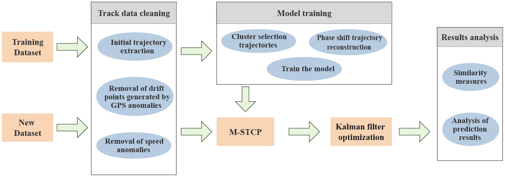
Figure 1 The M-STCP method architecture diagram consists of three parts: track data cleaning, model training, results analysis, and other intermediate processes.

3.1 Data preprocessing

Due to the complex maritime environment in real scenarios, the sensor equipment carried by fishing vessels often has problems such as signal loss and equipment failure, which will lead to problems such as incorrect reporting coordinates, reported data loss, and even crazy reporting of some equipment. Therefore, we need to preprocess the collected data and clean up the unwanted data. The original GPS trajectory data contains rich types of information, including ship ID, longitude (LON), latitude (LAT), heading, speed, time, ship type, tonnage, etc. For the ship trajectory prediction task, we want to carry out, only part of the information data is used, so we need to extract the trajectory of the ship. The extraction process of our required ship trajectory is as follows:

Step 1: Remove small fishing boat data. The results are more skewed because smaller boats are more susceptible to the environmental factors such as ocean weather;

Step 2: Remove the data of ship status as anchored and docked;

Step 3: Remove the same information in the data set due to repeated receipt of the same ship ID;

Step 4: Remove irrelevant data in the trajectory data to obtain the final trajectory.

Suppose the characteristics of the ship’s navigation trajectory at a certain time t can be expressed as:

$\begin{array}{ll}M(\text{t})=\left\{x_t,y_t,v_t,a_t\right\}& (1)\end{array}$

The target ship’s longitude, latitude, speed over the ground, and course over the ground are represented by the variables x_t, y_t,v_t,a_t respectively, at time t.

3.1.1 Remove GPS drift track points

When the GPS collects the longitude and latitude position information data of the ship back to the background server, there will often be abnormal points due to positioning abnormalities, that is, the ship’s trajectory has a large offset phenomenon in a short period, as shown in Figure 2, this phenomenon is GPS drift, and the point generated by GPS drift is called drift point.

FIGURE 2

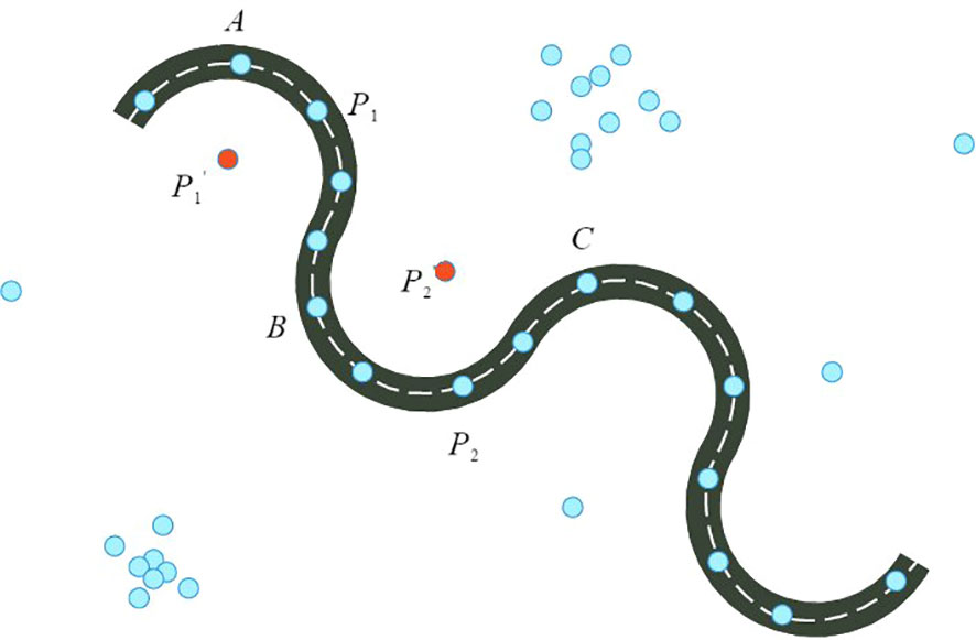
Figure 2 Schematic diagram of trajectory drift point.It shows the originally smooth points in a track, such as points A, B, C, P₁, P₂, and drift points due to GPS reception problems, such as points $P_1^{\text{'}}$ and $P_2^{\text{'}}$. What we want to remove is these drift points.

We detect drift points by whether the average velocity of the trajectory point and its neighboring trajectory point exceeds the threshold, and algorithm 1 displays the algorithmic procedure.

ALGORITHM 1. REMOVE DRIFT POINTS WHERE GPS POSITIONING IS INACCURATE.

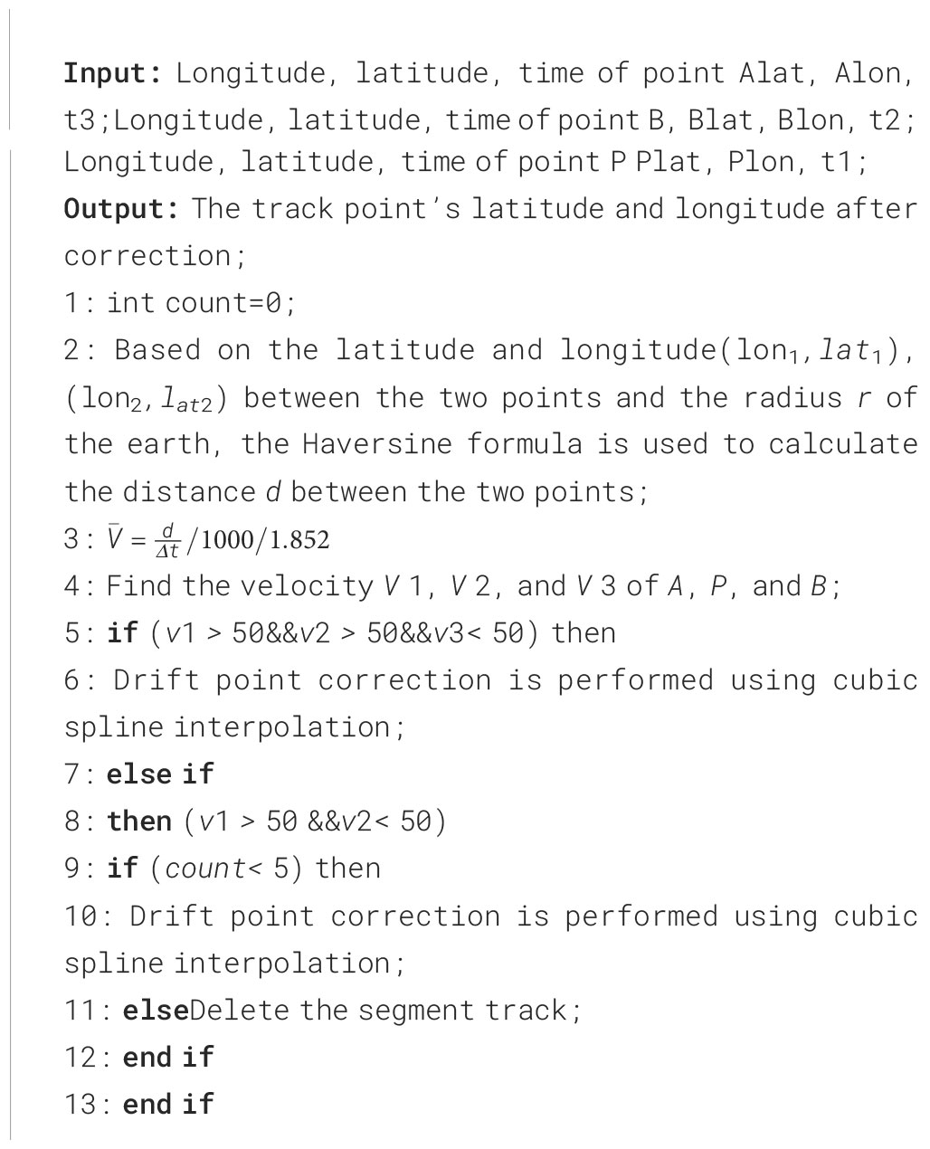
Algorithm 1. Remove drift points where GPS positioning is inaccurate..

Here is the precise procedure:

Step 1: Calculate the distance between adjacent volume track points. Through the Haversine formula in Eq(2), the distance can be directly calculated by the latitude and longitude coordinates of the two track points.

$\begin{array}{ll}d=2r{\sin }^{-1}\left(\sqrt{{\sin }^2\left(\frac{\text{la}{\text{t}}_2-\text{la}{\text{t}}_1}{2}\right)+\cos (\text{la}{\text{t}}_1)\cos (\text{la}{\text{t}}_2){\sin }^2\left(\frac{\text{la}{\text{t}}_2-\text{la}{\text{t}}_1}{2}\right)}\right)& (2)\end{array}$

Where d represents the distance between two points (unit: meters), r is the radius of the earth (take 6371km), (lon₁,lat₁) and (lon₂,lat₂)represent the latitude and longitude coordinates of the front and rear points, respectively.

Step 2: Average speed calculation. The average velocity between the two trajectory points is calculated by Eq(3).

$\begin{array}{ll}\overline{V}=\frac{d}{\Delta t}/1000/1.852& (3)\end{array}$

Where $\overline{V}$ is the average speed (unit: knots) between the two points, and δt is the time interval between the two points.

Step 3: Drift point judgment. The speed of ships near the port is about 30-40 knots, generally not exceeding 50 knots, so we set the normal speed threshold to 50 knots. Let the average speed between points A and P₁ be $\overline{\underset{\_}{V_1}}$, the average speed between points P₁ and B be $\overline{V_2}$, and the average speed between points, A and B be $\overline{V_3}$. If $\overline{V_1}$> 50, $\overline{V_2}$> 50 and $\overline{V_3}$< 50, only p is a drift point, and the point is corrected by the cubic spline interpolation method; if $\overline{V_1}$> 50, $\overline{V_2}$< 50, P₁ and point B are both drift points, then traverse the subsequent trajectory points to see if there are any drift points in the subsequent nodes, Stop traversing until the last point that is not a drift point. Count the number of continuous drift points. If it is less than 5, use cubic spline interpolation to correct the drift points. If it is greater than 5, delete this track directly.

3.1.2 Remove track points with abnormal velocity

Interpolation technology is a method that can effectively correct trajectory outliers and fill in missing data values and is widely used in various fields. The current interpolation techniques include piecewise linear interpolation, linear interpolation depending on speed and heading, piecewise cubic Hermite interpolation, cubic spline interpolation, etc. Because the time interval of the GPS receiving ship-related data is not uniform, the method of processing data into a sequence of equal time intervals by interpolation method not only has a huge workload but also may change the original data structure. Therefore, we use the basic principles of kinematics to correct the abnormal speed point, which is more accurate than the linear interpolation method. The algorithm is shown in algorithm 2.

Specific steps are as follows:

Step 1: Let the speed at the detection point be V. Calculate the average speed of a point before the detection point by Eq(3), denoted as $\overline{V_m}$, and calculate the average speed of the next point, denoted as $\overline{V_n}$.

Step 2: If the value of V is between $\overline{V_m}$ and $\overline{V_n}$, it indicates that the detection point is normal; otherwise, it is determined that the detection point is an abnormal point, and the corresponding threshold is set by the value of V, and the abnormal point is corrected by Eq(4).

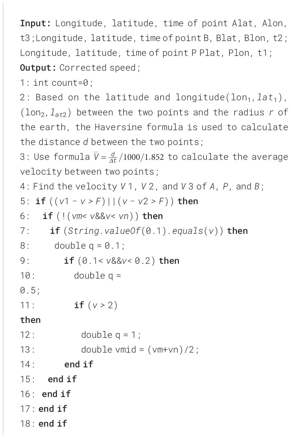
ALGORITHM 2. REMOVE ABNORMAL SPEED POINTS.

Algorithm 2. Remove abnormal speed points..

$\begin{array}{ll}{V}_{\text{mid}}=\frac{\overline{V_{\text{m}}}+\overline{V_{\text{n}}}}{2}& (4)\end{array}$

Step 3: Traverse all trajectory sequences to complete the detection and correction of abnormal speed.

3.2 M-STCP core method

M-STCP (Matrix-Based Ship trajectory Cleaning and Prediction) is a data cleaning and trajectory prediction method based on matrix neural networks. It leverages the advantages of matrix neural networks to efficiently clean ship trajectory data and accurately predict future ship trajectories. By applying matrix neural networks to the fields of data cleaning and trajectory prediction, M-STCP demonstrates capabilities in enhancing data processing efficiency and accuracy. The flow chart is shown in Figure 3. The core method of this method is described as follows.

FIGURE 3

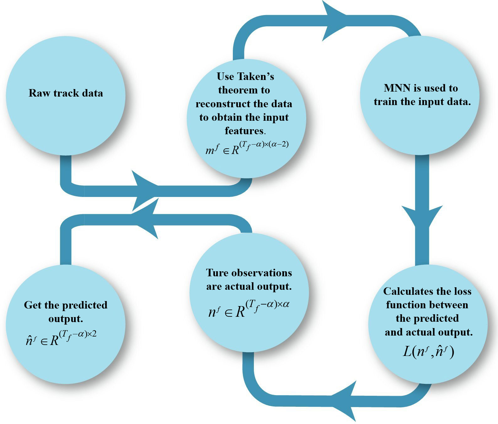
Figure 3 A trained model for ship trajectory prediction using a matrix neural network is shown. First, the original data is reconstructed into an input matrix m^f using Taken’s theorem, thus the test set and training set of the trajectory data set are separated. Secondly, the input matrix m^f is passed to the output layer through the matrix neural network. We predict an output of ${\widehat{n}}^f$ and an observation of n^f for the next step. The gradient of each layer is calculated using the loss function to facilitate the update of the circle matrix.

Each ship trajectory has its initial position $\left(\left(a_0^f,b_0^f\right)\right)$, even if the trajectory shape of the ship trajectory is different, it will be interpreted as a different trajectory due to the difference in the initial position. This also shows that there is a spatial bias in the trajectory dataset because the ship coordinates are described by latitude and longitude coordinates. To eliminate the spatial deviation, in the ship trajectory prediction, we can perform a phase shift reconstruction of the coordinates of all samples, and after the reconstruction, all the trajectory points are moved to the (0,0) point relative to the starting position of the trajectory, thereby eliminating the spatial deviation. For each time step t and each sample f from the original position $(a^f,b^f)(f>=0)$ reconstructed to the same starting point (0,0), the process is as in Eq (5):

$\begin{array}{ll}\left(a_t^f,b_t^f\right)=\left(a_t^f-a_0^f,b_t^f-b_0^f\right)& (5)\end{array}$

where $\left(a_0^f,b_0^f\right)$ represents the latitude and longitude coordinates of the fth sample in the first time step.

In this way, we can unify the starting point of all trajectories to the same location, eliminating the spatial bias caused by different starting point locations, to make trajectory prediction more efficient.

In ship trajectory prediction, we use matrix neural networks for autoregressive or sliding window prediction frameworks. Data embedding reconstruction for time series is also referred to as Taken’s theorem. According to Taken’s theorem, the size is chosen to be α and a regular interval of β to reconstruct the time series, thus the original time series’ properties are preserved in the reconstructed time series. The given ship trajectories are binary sequences, and each trajectory data is embedded as a matrix of size $(T_f-\alpha )\times (\alpha \times 2)$, and each data point contains two feature information of latitude and longitude (a_t,b_t). The time series data takes the location coordinate information as an input point in chronological order, and then forms an input matrix $m_t^f$. Each row of the input matrix contains two eigenvalues, latitude and longitude. Starting from the α + 1st position coordinate to the last position coordinate as a data point, the output matrix is formed. Each row of the output matrix also contains two eigenvalues. The input matrix and output matrix form are shown in Eq(6): (t ≥ 0)

$\begin{array}{ll}{\mathbf{m}}_t^f=\left[\begin{array}{cc}{a}_{t+1}^f& a_{t+1}^f\\ a_{t+2}^f& b_{t+2}^f\\ ⋮& ⋮\\ a_{t+\alpha }^f& b_{t+\alpha }^f\end{array}\right],{\mathbf{n}}_t^f=\left[\begin{array}{cc}{a}_{t+(\alpha +1)}^f& b_{t+(\alpha +1)}^f\\ ⋮& ⋮\end{array}\right]& (6)\end{array}$

In this way, we can convert the trajectory data into matrix form and use it to train a matrix neural network model to achieve predictions of ship trajectories.

When dealing with problems involving spatial correlation such as ship trajectory coordinates, if the traditional neural network input vector sum is used, information will be lost. As a result, matrix neural networks are better suited to handle these issues. The mapping between MNN layers and layers is defined in Eq(7).

$\begin{array}{ll}{\mathbf{\text{X}}}^{l+1}=\sigma ({\mathbf{\text{W}}}^l{\mathbf{\text{X}}}^l{\mathbf{\text{V}}}^{\text{l}T}+{\text{B}}^l)& (7)\end{array}$

The expanded form is as follows:

$\begin{array}{ll}\left[\begin{array}{c}{x}_{1f}^{l+1}\\ x_{2f}^{l+1}\\ \\ x_{pf}^{l+1}\end{array}\right]=\sigma \left(\left[\begin{array}{cccc}{w}_{11}^l& w_{12}^l& \dots & w_{1n}^l\\ w_{21}^l& w_{12}^l& \dots & w_{2n}^l\\ & & & \\ w_{p1}^l& w_{p2}^l& \dots & w_{pn}^l\end{array}\right]\left[\begin{array}{c}{x}_{1f}^l\\ x_{2f}^l\\ \\ x_{nf}^l\end{array}\right]+\left[\begin{array}{c}{b}_{1f}^{l+1}\\ b_{2f}^{l+1}\\ \\ b_{pf}^{l+1}\end{array}\right]\right)& (8)\end{array}$

Among them, X^l is the matrix variable of the L layer, X^l+1 is the output in the L layer, W, X, V, B are matrices with compatible dimensions, B^l is the offset of the current layer, and σ()is the activation function. The matrix form of the data can be maintained by Eq(8). Through the changes of W(l), X(l), and V (l), the matrix form of the hidden layer can be reconstructed. The specific matrix change process is shown in Eq(9):

$\begin{array}{ll}{W}^l\in R^p{}^{\times q}\times X^l\in R^a{}^{\times b}\times V^{lT}\in R^b{}^{\times q}=X^l{}^{+1}\in R^p{}^{\times q}& (9)\end{array}$

The matrix variation formula of a matrix neural network is shown the matrix transformation process from input matrix X^l to output matrix X^l+1, which is different from traditional vector-based input. Also shown is the matrix transformation for the ith window from time t to t + α, which gives the latitude and longitude of the ship’s trajectory. Among them, the matrix dimension is changed from a × b to p × q by the dimension dot product of the input matrix.

The definition of the ship trajectory indicates that the input data m^f of the matrix neural network is a three-dimensional tensor of size, that is, the number of sliding windows for each input data is T_f - α), each The size of the input unit is α × 2. The number of each output data sliding window of the output data is also, and the size of each output unit is 2. That is, we need to find the mapping relationship that changes the size of the matrix from α × 2 to 2, that is, f: ℝ^a×2 → ℝ². To lessen the discrepancy between the supplied output n^f and the network output ${\widehat{n}}^f$, we adopt Eq(10) for learning.

$\begin{array}{ll}\underset{W}{\min }{\displaystyle \sum _{f=1}^{N}L}({\widehat{n}}^f,n^f)={\displaystyle \sum _{f=1}^N\frac{\mathbf{1}}{T_f-\alpha }}{\Vert {\mathbf{\text{n}}}^f-{\widehat{\mathbf{\text{n}}}}^f\Vert }_2^2& (10)\end{array}$

3.3 Kalman filter optimization

The ship’s track in space is some time series data. Because our track data is measured by various sensors, there will be some unavoidable errors. To ensure the accuracy of trajectory prediction, we need to smooth the data. Rudolph E. Kalman put forward the Kalman filter in 1960 and gave a new method to solve the prediction problem. Kalman filter takes into account the possible uncertainty in the prediction process and estimates the optimal result through incomplete accurate prediction models and incomplete accurate measurement results. The prediction equation includes the system’s status right now and the uncertainty of the system. The specific process of KF is to evaluate the prediction equation and correction equation through recursion. The prediction equation estimates the current state and uncertainty of the system. The correction equation uses the measured current state quantity of the system to update the estimation. It should be noted that in KF, we assume that both system uncertainty and measurement uncertainty follow a normal distribution.

The prediction equation of Kalman filter is:

$\begin{array}{ll}{\widehat{x}}_k^{-}=\text{A}·{\widehat{x}}_{k-1}+\text{B}·{\mathit{\text{u}}}_{k-1}& (11)\end{array}$

$\begin{array}{ll}{\text{P}}_k^{-}=\text{A}·{\text{R}}_{k-1}·{\text{A}}^T+\mathit{\text{Q}}& (12)\end{array}$

In Eq(11) ${\widehat{X}}_k^{-}$ represents a prior estimate at time k, A is the state matrix, ${\widehat{X}}_{k-1}$ represents the estimated value at k − 1 time, B represents the control matrix, u_k−1 represents the control variable at the moment. In Eq(12) ${\text{P}}_k^{-}$ represents the prior error covariance, A represents the state matrix, ${\text{P}}_{k-1}$ represents the error covariance at k − 1, and Q represents the covariance of process noise. The correction equation of the

Kalman filter is:

$\begin{array}{ll}\begin{array}{l}{K}_k= \frac{P_k^{-}·H^T}{H·P_k^{-}·H^T+R} \hfill \end{array}& (13)\end{array}$

$\begin{array}{ll}{\widehat{x}}_k={\widehat{x}}_k^{-}+{\text{K}}_k·(z_k-\mathbf{\text{H}}·{\widehat{x}}_k^{-})& (14)\end{array}$

$\begin{array}{ll}{\text{P}}_k=(\mathbf{\text{I}}-{\mathbf{\text{K}}}_k·\mathbf{\text{H}})·{\mathbf{\text{P}}}_k^{-}& (15)\end{array}$

In Eq(13), K_krepresents the Kalman ga in, H represents the observation matrix, and R represents the error covariance of the measurement process. In Equation (14),${\widehat{X}}_k$ represents a posterior estimate, that is, the optimal estimate we need, Z_krepresents the measured value at time k. In Eq(15), P_krepresents the update error covariance at time k. The covariance matrices of process noise and measurement noise are represented by the matrices Q and R in the Kalman filter, respectively. The larger the value of Q, the more trust we have in the measured results, the greater the value of R will be, and the more trust we have in the estimated results.

When the M-STCP method is combined with the Kalman filter for ship trajectory prediction, the Kalman filter needs to be set including the state transition equation, measurement equation, initial state, and covariance matrix. First, a dynamic trajectory forecast model is determined by the vessel’s historical trajectory. Then, the observation values such as position and speed information are input into the matrix neural network, and the state estimation is carried out to obtain the predicted value of the ship’s state at that moment. The predicted value is then corrected using a Kalman filter to obtain a ship condition estimate that is closer to the real value. The specific implementation is shown in algorithm 3 .

We can define the state of a ship as a four-dimensional vector X(k) ={x_k, y_k, v_xk, v_xyk}, where x_kand y_krepresent the ship’s position on a planar coordinate system, and v_xkand v_ykrepresent the ship’s velocity in the x-axis and y-axis directions. This state variable evolves between adjacent temporal steps, so we can use a transition matrix A to describe the evolution of state variables in each temporal step. In particular, under the assumption that the time step is dt, the transition matrix can be defined as:

$\begin{array}{ll}A=\left[\begin{array}{cccc}1& 0& dt& 0\\ 0& 1& 0& dt\\ 0& 0& 1& 0\\ 0& 0& 0& 1\end{array}\right]& (16)\end{array}$

The Q process noise covariance matrix represents the uncertainty or noise of the state variable during the forecast. Ships can be affected by factors such as wind and currents while sailing, so we can build a random walking pattern. Then, depending on the location of the ship, we can define the Q corresponding to where t is the sampling interval.

$\begin{array}{ll}Q=\left[\begin{array}{cccc}\frac{1}{3}(\frac{\Delta t^3{v}^2}{L^2})& 0& \frac{1}{2}(\frac{\Delta t^{2}v}{L})& 0\\ 0& \frac{1}{3}(\frac{\Delta t^3{v}^2}{L^2})& 0& \frac{1}{2}(\frac{\Delta t^{2}v}{L})\\ \frac{1}{2}(\frac{\Delta t^{2}v}{L})& 0& \Delta t& 0\\ 0& \frac{1}{2}(\frac{\Delta t^{2}v}{L})& 0& \Delta t\end{array}\right]& (17)\end{array}$

Observe the value of the noise covariance matrix R We measure the position and speed data of the ship, record the measurement data and observe the error to obtain the value of the R matrix, and you can set it to:

$\begin{array}{ll}R=\left[\begin{array}{cccc}{\sigma }_{xk}^2& 0& 0& 0\\ 0& {\sigma }_{yk}^2& 0& 0\\ 0& 0& {\sigma }_{v_{xk}}^2& 0\\ 0& 0& 0& {\sigma }_{v_{yk}}^2\end{array}\right]& (18)\end{array}$

ALGORITHM 3. KALMAN FILTER OPTIMIZATION.

Algorithm 3. Kalman filter optimization..

4 Experiments and analysis

In this section, we leverage a substantial amount of actual ship trajectory data to validate the model’s efficacy. The prediction results of M-STCP, GRU models (Han et al., 2019), and long short-term memory networks (Tang et al., 2022) are compared. It is demonstrated that our methodology accurately predicts time series data by a comparative study of the experimental findings.

4.1 Data description

To ensure the validity of trajectory prediction, we utilize real trajectory data. The ship tracking data used in this article is from the Wenzhou Fishing Vessel Safety and Rescue Center, which contains about 5 million tracks in Jiangsu and Zhejiang in 2016. The GPS data collection cycle is 15-30 minutes, the data set size is approximately 70GB, and it contains about 40 million pieces of trajectory data. Oracle Database is used for data storage. In Table 1, a sample of the GPS data are displayed. To obtain the density/frequency feature of the trajectory data, we plot ship trajectories every four months in the same heatmap respectively. The space heat map is shown in Figure 4.

TABLE 1

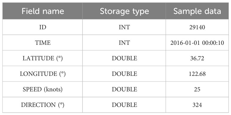
Table 1 GPS track data storage format and data sample.

FIGURE 4

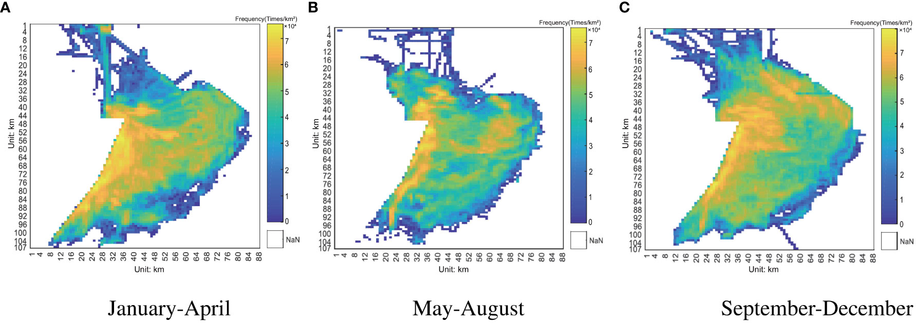
Figure 4 Visualization of GPS raw data from Zhoushan fishery, China. After the sea zone is gridded into cells, horizontal and vertical coordinates are established, and the number of vessel occurrences in each cell is accumulated. Each cell is 10 km long. The yellow area denotes the area with a higher density of the trajectory, and the darker the hue, the greater the density of the trajectory. The blue line represents the ship’s trajectory.

The data distribution after extraction and processing of the original ship trajectory and anomaly point cleaning is shown in Figure 5. The trajectory points set in this paper have a longitude range of [119.6,131.0], a latitude range of [22.0,33.8], a direction range of [0.0,360.0], and a velocity range of [0.0,25.0].

FIGURE 5

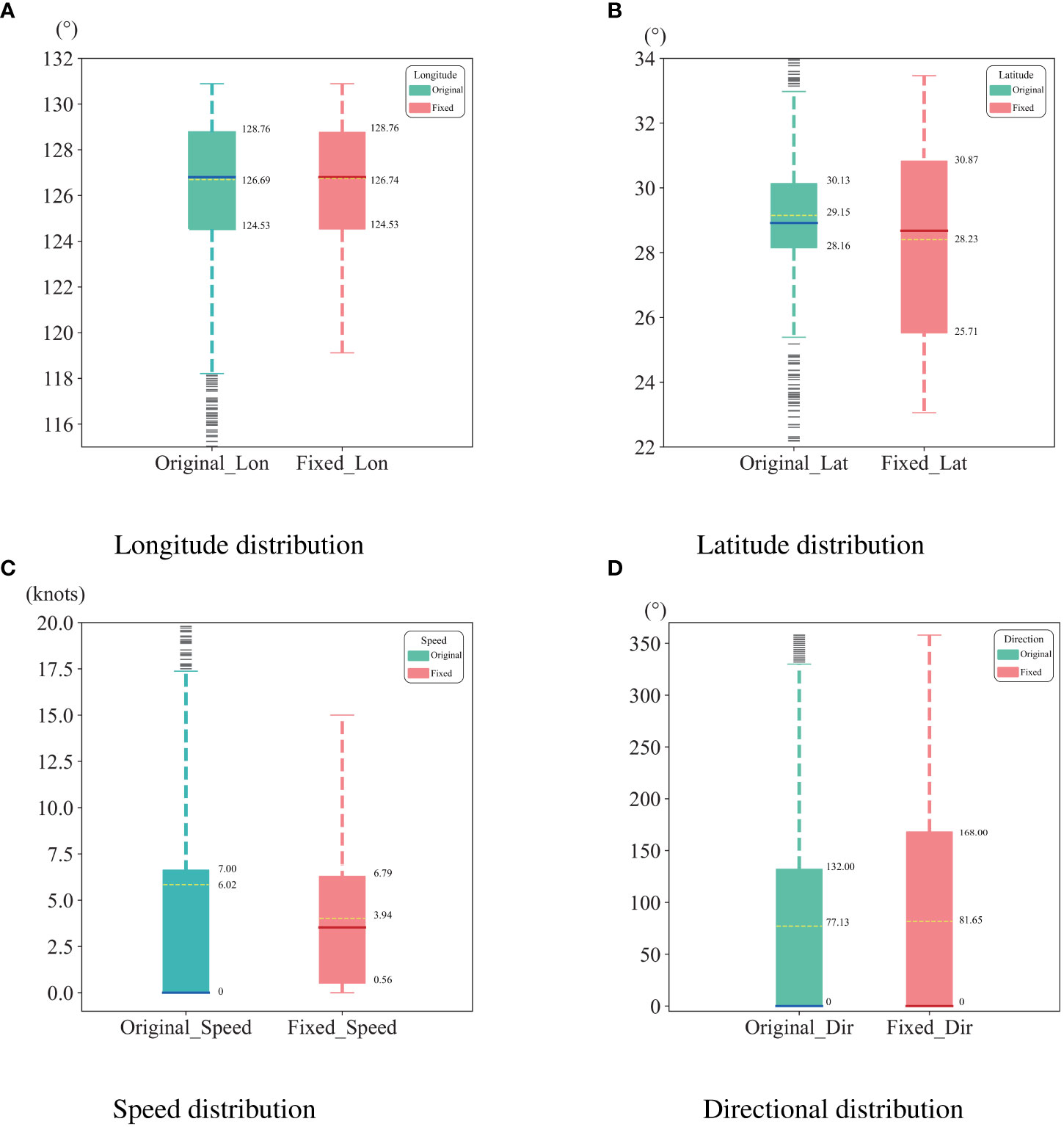
Figure 5 The distribution of longitude, latitude, velocity, and direction after removing anomalies data in the trajectory. The continuous blue line represents the median, the yellow dashed line represents the 25% quantile, and the 75% quantile is also labelled.

Due to the complex ship motion pattern in the real data, the ship’s trajectory is not single linear, we cluster it using the DBSCAN technique based on density. According to the collected large number of ship trajectory data, the corresponding characteristics such as ship number and ship steering angle are selected, and the ship trajectories with similar patterns are regarded as the same cluster through DBSCAN. The key to the clustering algorithm is to adjust the two parameters of the Eps radius and the minimum number of MinPts samples. Following experimental tests, our Epsilon is set to 0.4 and MinPts to 8, optimizing the clustering effect. The results of the ship trajectory clustering are displayed in Figure 6, including the number of the four clusters and the approximate direction of the trajectory. Although there are some anomalous trajectories in the clustering results, we can see significant differences between each cluster.

FIGURE 6

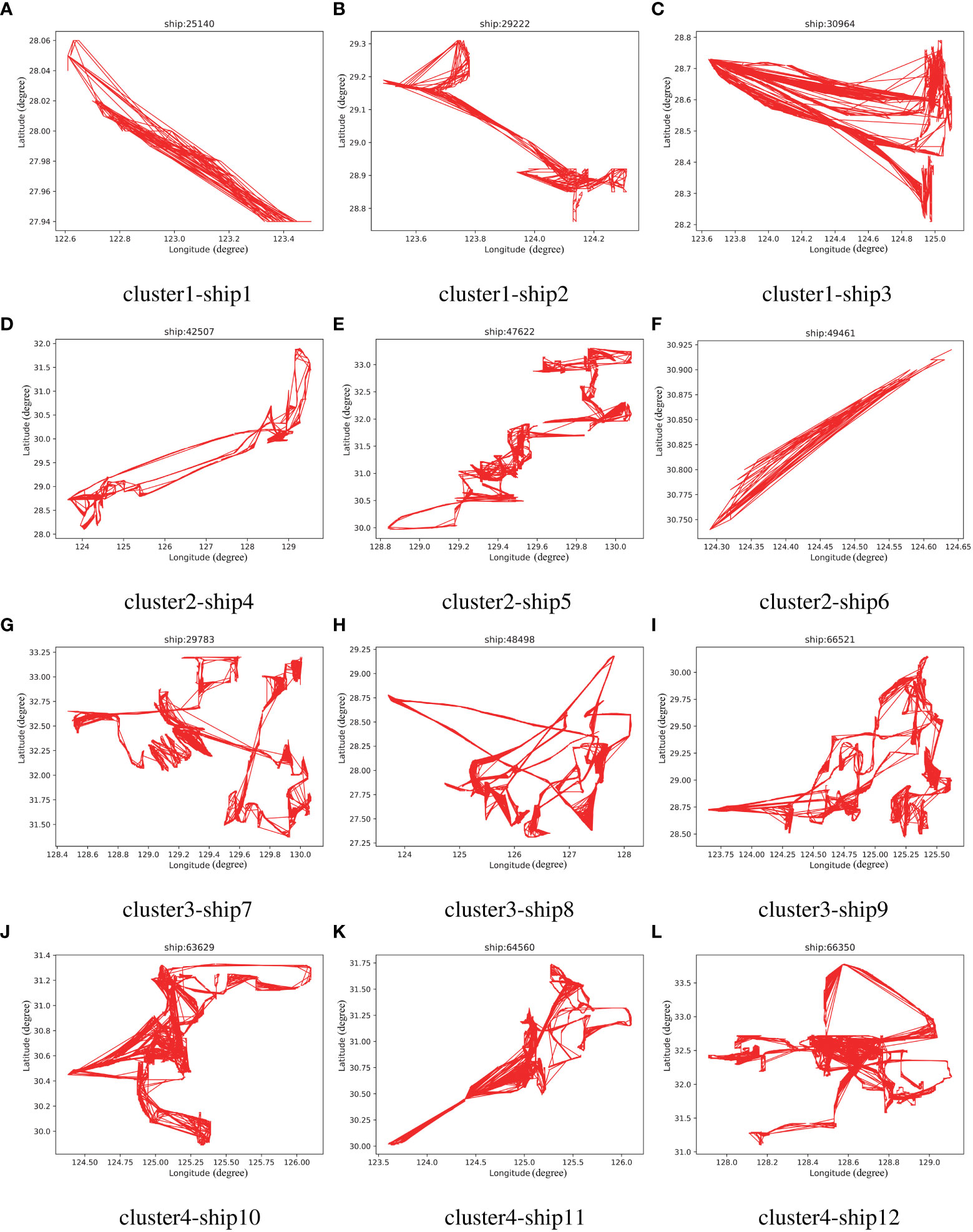
Figure 6 The result of trajectory clustering. (A-C) are cluster 1, (D-F) are cluster two, (G-I) are cluster three, and (J-L) are cluster four.

4.2 Performance evalution

For neural networks, the value range of the input features is too large to cause the gradient descent algorithm to converge slowly or difficult to converge, so we normalize the input features, scale the data to the range of [0,1], and limit the value range to a certain range, to eliminate the adverse effects caused by the data, accelerate the model convergence speed, and enhance the model’s generalizability and stability. The normalization formula is shown in Eq(16):

$\begin{array}{ll}{x}_{norm}=\frac{x-x_{\min }}{x_{\max }-x_{\min }}& (19)\end{array}$

where x is the original data, x_min and x_max are the minimum and maximum values of the data in the sample, respectively, and x_normis the normalized data.

At present, the mainstream methods in the field of ship trajectory prediction include recurrent neural networks, deep learning, LSTM, GRU, etc. We compare these methods, as shown in Table 2. We can see that MNN is a new method of predicting trajectory, which has greater efficiency and data processing capacity than the traditional neural network method. Comparison of mainstream methods for ship trajectory prediction.

TABLE 2

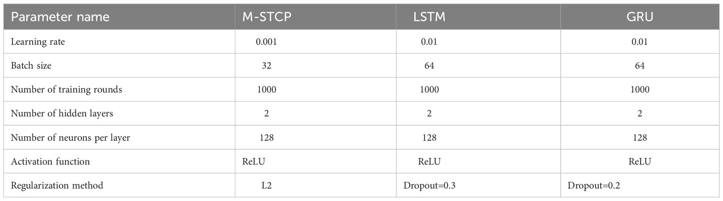
Table 2 Parameter values of M-STCP, LSTM, GRU models.

Parameter selection is an important factor influencing prediction outcomes. A number of neurons and a greater number of layers can extract more information about the vessel’s track characteristics, but excessive complexity can also lead to overflow. The experiments use the RMSProp optimizer, a method to optimize adaptive learning rate and stochastic gradient descent. It can efficiently address oscillation and instability issues in traditional gradient descent algorithms. After experimental verification and parameter comparison, the M-STCP architecture comprises the following elements: input layer, matrix multiplication layer, non-linear transformation layer, loop layer and output layer. The input layer is used to input ship trajectory data into the neural network; The matrix multiplication layer converts the input trajectory data into matrix form for input to the next layer; The nonlinear change layer applies nonlinear functions to each element of the matrix to enhance the expressiveness of the model; The recurrent layer will apply the recurrent neural network to process the matrix to better capture the time series information in the trajectory data. The output layer produces the last line of the matrix subsequent to the prediction. Xavier initialization and ReLU activation are used to initialize the parameters. The loss function selects the average square error to reduce the error between the expected outcome and the actual value. In the case that the default learning rate is 0.001, in order to find the optimal batch size and the number of neurons, we conduct experimental comparisons and determine that the batch size is 32 and the number of neurons is 128. Supplementary parameter selections for the remaining two methods are presented in Table 3. The details of experimental hardware configuration used in this paper are shown in Table 4.

TABLE 3

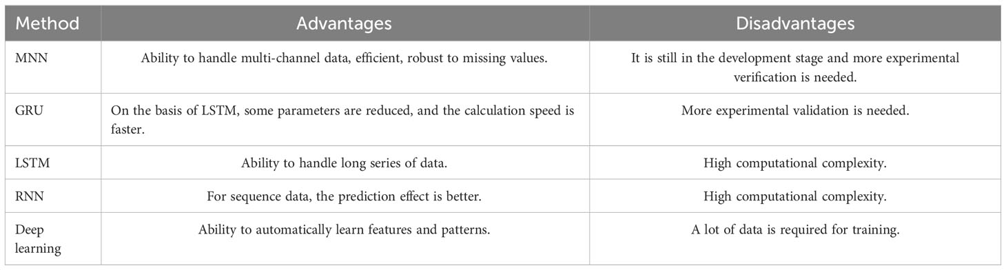
Table 3 The hardware configuration required for the experiment.

TABLE 4

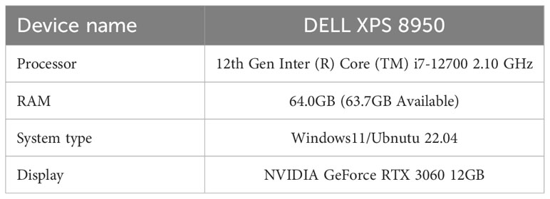
Table 4 Comparison of prediction performance by using M-STCP, GRU, LSTM in terms of MAPE, MAE, RMSE.

For additional evidence that the suggested model is workable and successful, we use 70% of the experimental dataset as the training set and 30% as the test set. The results of the M-STCP method and Kalman filter processing were compared and analyzed with the prediction results of the LSTM model and the GRU (Han et al., 2021) model, and the experimental results were verified by the test set. In the experiment, we selected two sets of data sets for comparison to compare the prediction effects of the three methods on simple and complex ship trajectories. The first set of datasets contains relatively complex, curved ship trajectory data; The second set of data includes simpler ship trajectory data. In Figure 7, the experimental outcomes are displayed. Figure 7’s a and c show that at the beginning of the ship trajectory, only the prediction results of the M-STCP method processed by KF are more accurate, the M-STCP method has the same movement trend as the ship trajectory, but due to the influence of noise, there is a deviation in latitude and longitude, and the performance of the LSTM model is the worst. Although the prediction results of the three models are roughly the same as those of the real ship trajectory, M-STCP is better than LSTM and GRU in the trajectory prediction performance of the ship with large changes in the course of the ship. In Figure 7, it is visible from b that for simple trajectories, although the prediction results of LSTM and GRU have the same motion trend as the real trajectory, the position information has a large deviation, while the M-STCP method and the real trajectory not only have the same motion trend but also similar position information. This is because although LSTM and GRU have the strong fitting ability, they are also prone to overfitting. The matrix neural network adopts the matrix decomposition method to reduce the number of parameters, effectively reduces the risk of overfitting, and retains the spatiotemporal correlation in the trajectory data when predicting the trajectory of the ship, which also makes its prediction effect better than that of the traditional neural network.

FIGURE 7

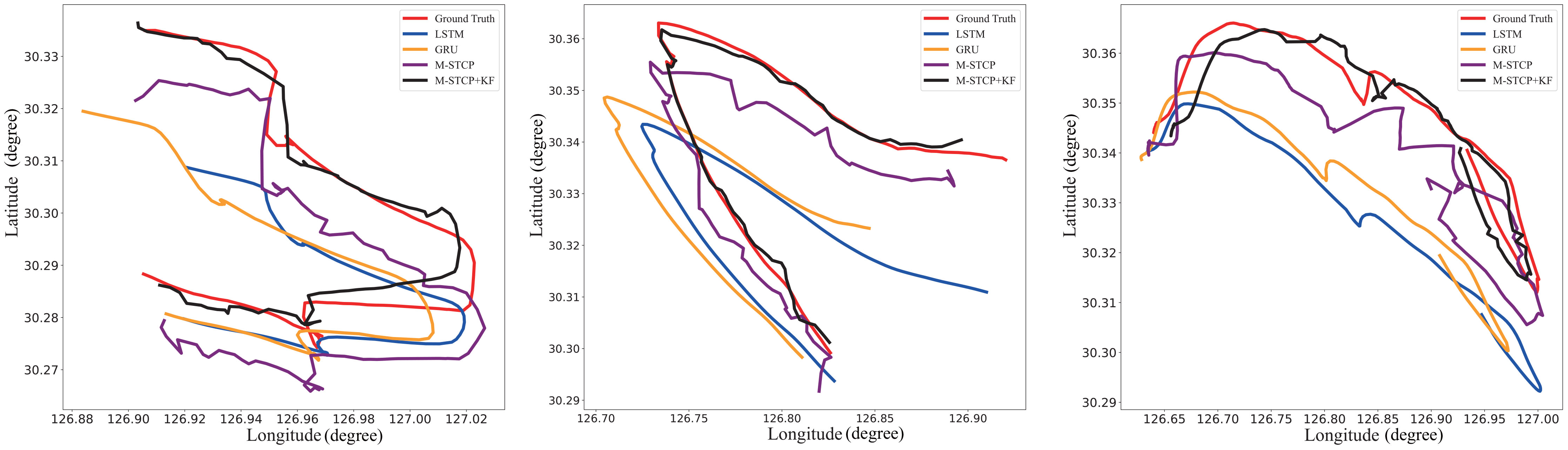
Figure 7 The results of predicting the latitude and longitude of ship trajectory by using M-STCP, LSTM, GRU and M-STCP combined with Kalman filter.

To provide a more precise demonstration of the deviation between predicted and actual results, we have chosen to examine 100 sets of ship trajectories through three different methods, ultimately presenting their longitude and latitude error scatter plots in Figure 8. The M-STCP method’s error in latitude and longitude can be found to be lower than those of the other two approaches, and the error of the M-STCP method after the Kalman filter treatment is further reduced, and the GRU model has the lowest prediction accuracy. This also proves the good performance of M-STCP in ship trajectory prediction.

FIGURE 8

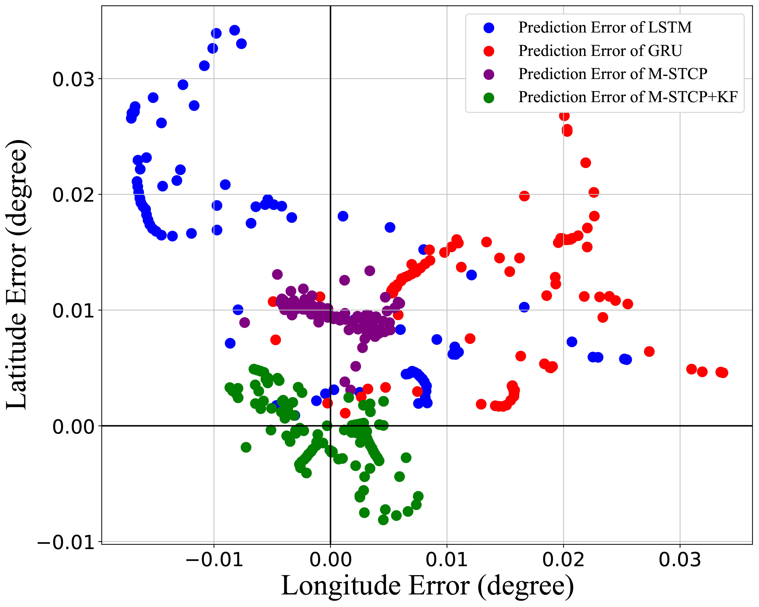
Figure 8 The ship trajectory error distribution is optimized by LSTM,GRU,M-STCP, and M-STCP after Kalman filter.

For the prediction results of the experiment, We employ evaluation metrics including root mean square error RMSE, mean absolute error MAE, mean absolute percentage error MAPE. All four evaluation methods are that smaller values indicate more accurate predictions from the model. where y_irepresents the true trajectory value and ${\widehat{y}}_i$ represents the predicted value of the trajectory. As stated in Table 5, the specific values are tabulated, and the histogram is shown in Figure 9. Taking MAPE and MSE as indicators to evaluate the prediction results, it can be seen that the M-STCP value is the smallest and the prediction effect is the best, followed by LSTM and GRU have the worst performance. Using MAE and RMSE as indicators to evaluate the prediction results, M-STCP has the best prediction effect, GRU and LSTM values were similar and higher than those of M-STCP method. In summary, the value of the M-STCP method is smaller than that of the other two models under the three evaluation criteria, which indicates that M-STCP has a high precision than the LSTM and GRU models.

TABLE 5

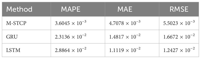
Table 5 Comparison of mainstream methods for ship trajectory prediction.

FIGURE 9

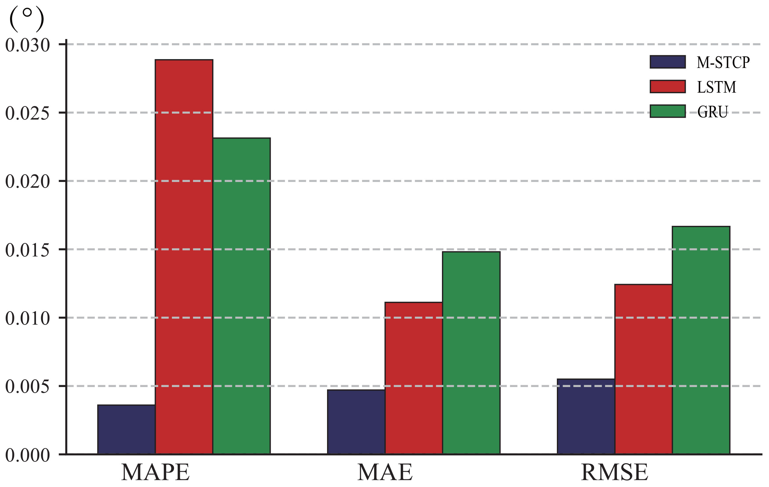
Figure 9 The evaluation results of the three methods were histogram using the evaluation criteria of MAPE, MSE and RMSE.

$\begin{array}{ll}\text{MAPE}=\frac{100\%}{n}{\displaystyle \sum _{i=1}^n\left|\frac{{\widehat{y}}_i-y_i}{y_i}\right|}& (20)\end{array}$

$\begin{array}{ll}\text{MAE}=\frac{1}{n}{\displaystyle \sum _{i=1}^n\left|yi-{\widehat{y}}_i\right|}& (21)\end{array}$

$\begin{array}{ll}\text{RMSE}=\sqrt{\frac{1}{m}{\displaystyle \sum _{i=1^{}}^m{(y_i-{\widehat{y}}_i)}^2}}& (22)\end{array}$

5 Conclusion and future works

In this paper, we introduce an online ship track cleaning and prediction algorithm M-STCP based on matrix neural network. Matrix neural networks, or MNNs, can be applied to predict future ship trajectories using clustered GPS ship trajectory data. The reliability of the dataset is also a critical part of prediction accuracy. Due to sensor acquisition problems, the data set we use may contain some noise and invalid trajectory points, and by cleaning the data set and using Kalman filter, we can obtain a data set closer to the real ship trajectory, and also make the prediction results more realistic and effective. We compare the results of M-STCP predictions of ship trajectories with LSTM and GRU models. To improve the accuracy of the experimental findings, we first extracted ship trajectories with similar behavior patterns in the original trajectory data by clustering method, and then processed them to remove anomalies and invalid values. Predict the future trajectory of ships by using the M-STCP method. We selected three evaluation metrics to evaluate the forecasting methodology. In terms of prediction accuracy, LSTM is 84.27%, GRU is 87.62%, while M-STCP method can reach 88.52C%, which can be improved to 89.44% after Kalman filter noise reduction.

M-STCP’s ship trajectory prediction accuracy is higher than that of GRU and LSTM, as evidenced by the experimental results. Ship trajectories can be regarded as a series of time trajectory data, and matrix neural networks have important advantages in addressing time series problems. Based on a matrix neural network, we maintain the spatial correlation between the trajectory data by eliminating the spatial offset in the original dataset so that all ship trajectories start from the same starting position. Matrix neural networks can effectively process multi-dimensional time series data, making them capable of performing multi-scale analysis on data and enhancing data expression capabilities. By doing this, neural networks can learn the input data’s features more efficiently and process multi-dimensional input and output data with greater efficiency. Matrix neural networks convert sequence data into matrix or tensor form, enabling parallel computing, speeding up the training process, and addressing the long-term dependency problem by doing so. In contrast, the biggest advantage of matrix neural networks is that they can efficiently process large-scale data and have a fast training speed, but their accuracy is easily affected by noise. Sequence data handling with good stability and solving long-term dependencies through control units can be done by LSTM and GRU using their control units. GRU and LSTM’s internal structure is both complex and difficult to interpret. When time series data are long, the problem of disappearing or exploding the gradient arises and the computation time is long. Setting parameters and adjusting the number of layers is a challenge for all three methods, and they require high computing resources. Matrix neural networks can often provide better prediction performance than traditional recurrent neural networks like GRU and LSTM in sequence modeling tasks, including ship trajectory prediction.

In addition, there are other influencing factors, such as wind wave and tide intensity on the ocean, visibility at sea, and the width and depth of the waterways in this sea area, which were not considered in this study. These influencing factors may contribute to the prediction results of matrix neural networks. In future work, we can use other factors that affect the trajectory of ships, such as the strength of wind and waves and tides on the ocean, as input characteristics for prediction. In further work, we will improve the accuracy of long-term trajectory prediction based on improving the calculation accuracy, which will help ships navigate traffic problems with early warning.

Data availability statement

The raw data supporting the conclusions of this article will be made available by the authors, without undue reservation.

Author contributions

SG and MS contributed to the concept and design of the study, writing a first draft. MS and XM organized the experimental data, designed the experimental methods, and analyzed the experimental data. XM contributed to the design verification and verification of experiments. SW plotted the picture from the experiment. HX contributed to the design verification and verification of experiments. CL contributed to the review and revision of papers. All authors contributed to the article and approved the submitted version.

Funding

This research was funded by the Shandong Province Natural Science Foundation. The grant number is ZR2020QF028.

Conflict of interest

The authors declare that the research was conducted in the absence of any commercial or financial relationships that could be construed as a potential conflict of interest.

Publisher’s note

All claims expressed in this article are solely those of the authors and do not necessarily represent those of their affiliated organizations, or those of the publisher, the editors and the reviewers. Any product that may be evaluated in this article, or claim that may be made by its manufacturer, is not guaranteed or endorsed by the publisher.

References

Aggarwal C. C. (2018). Neural networks and deep learning. Springer 10, 3. doi: 10.1007/978-3-319-94463-0

CrossRef Full Text | Google Scholar

Bao K., Bi J., Gao M., Sun Y., Zhang X., Zhang W. (2022). An improved ship trajectory prediction based on ais data using mha-bigru. J. Mar. Sci. Eng. 10, 804. doi: 10.3390/jmse10060804

CrossRef Full Text | Google Scholar

Chen S., Zhang J., Meng F., Wang D. (2021). A markov chain position prediction model based on multidimensional correction. Complexity 2021. doi: 10.1155/2021/6677132

CrossRef Full Text | Google Scholar

Dalsnes B. R., Hexeberg S., Flaten A. L., Eriksen B.-O. H., Brekke E. F. (2018). “The neighbor course distribution method with gaussian mixture models for ais-based vessel trajectory prediction,” in 2018 21st international conference on information fusion (FUSION) (Cambridge, UK: IEEE), 580–587.

Google Scholar

El-Rabbany A. (2002). Introduction to GPS: the global positioning system (United States of America: Artech house).

Google Scholar

Fossen S., Fossen T. ,. I. (2018). exogenous kalman filter (xkf) for visualization and motion prediction of ships using live automatic identification system (ais) data. MODELING IDENTIFICATION AND CONTROL 39, 233–244. doi: 10.4173/mic.2018.4.1

CrossRef Full Text | Google Scholar

Gao J., Guo Y., Wang Z. (2017). “Matrix neural networks,” in Advances in neural networks - ISNN 2017 (Springer), 313–320.

Google Scholar

Gao D.-w., Zhu Y.-s., Zhang J.-f., He Y.-k., Yan K., Yan B.-r. (2021). A novel mp-lstm method for ship trajectory prediction based on ais data. Ocean Eng. 228, 108956. doi: 10.1016/j.oceaneng.2021.108956

CrossRef Full Text | Google Scholar

Guo S., Liu C., Guo Z., Feng Y., Hong F., Huang H. (2018). “Trajectory prediction for ocean vessels base on k-order multivariate markov chain,” in International Conference on Wireless Algorithms, Systems, and Applications. Part of the Lecture Notes in Computer Science book series (LNTCS, volume 10874). 140–150 (Springer, Cham).

Google Scholar

Han P., Wang W., Shi Q., Yang J. (2019). “Real-time short-term trajectory prediction based on gru neural network,” in In 2019 IEEE/AIAA 38th digital avionics systems conference (DASC) (San Diego, CA, USA: IEEE), 1–8.

Google Scholar

Han P., Wang W., Shi Q., Yue J. (2021). A combined online-learning model with k-means clustering and gru neural networks for trajectory prediction. Ad Hoc Networks 117, 102476. doi: 10.1016/j.adhoc.2021.102476

CrossRef Full Text | Google Scholar

Hu Q., Jiang Y., Zhang J., Sun X., Zhang S. (2015). Development of an automatic identification system autonomous positioning system. Sensors 15, 28574–28591. doi: 10.3390/s151128574

PubMed Abstract | CrossRef Full Text | Google Scholar

Imran M., Ayob A., Jamaludin S. (2022). Applications of artificial intelligence in ship berthing: A review. Indian J. Geo-Marine Sci. (IJMS) 50, 855–863.

Google Scholar

Jiang B., Guan J., Zhou W., Chen X. (2019). Ship trajectory prediction algorithm based on polynomial kalman filter. Signal Process. 35, 741–746. doi: 10.16798/j.issn.1003-0530.2019.05.002

CrossRef Full Text | Google Scholar

Koohang A., Sargent C. S., Nord J. H., Paliszkiewicz J. (2022). Internet of things (iot): From awareness to continued use. Int. J. Inf. Manage. 62, 102442. doi: 10.1016/j.ijinfomgt.2021.102442

CrossRef Full Text | Google Scholar

Lam J. S. L., Cullinane K. P. B., Lee P. T.-W. (2018). The 21st-century maritime silk road: challenges and opportunities for transport management and practice. Transport Rev. 38, 413–415. doi: 10.1080/01441647.2018.1453562

CrossRef Full Text | Google Scholar

Li X., Zhou S., Yin K., Liu H. (2021). Measurement of the high-quality development level of China’s marine economy. Mar. Economics Manage. 4 (1), 23–41. doi: 10.1108/MAEM-10-2020-0004

CrossRef Full Text | Google Scholar

Liu R. W., Yuan W., Chen X., Lu Y. (2021). An enhanced cnn-enabled learning method for promoting ship detection in maritime surveillance system. Ocean Eng. 235, 109435. doi: 10.1016/j.oceaneng.2021.109435

CrossRef Full Text | Google Scholar

Liu L., Zhang Y., Hu Y., Wang Y., Sun J., Dong X. (2022). A hybrid-clustering model of ship trajectories for maritime traffic patterns analysis in port area. J. Mar. Sci. Eng. 10, 342. doi: 10.3390/jmse10030342

CrossRef Full Text | Google Scholar

Lu C.-H. (2018). Context-aware service provisioning via agentized and reconfigurable multimodel cooperation for real-life iot-enabled smart home systems. IEEE Trans. Systems Man Cybernetics: Syst. 50, 2914–2925. doi: 10.1109/TSMC.2018.2831711

CrossRef Full Text | Google Scholar

Nguyen T. D. (2020). “Evaluation of the accuracy of the ship location determined by gps global positioning system on a given sea area,” in Journal of Physics: Conference Series, Engineering and Innovative Technologies. Vol. 1515. 042010 (IOP Publishing).

Google Scholar

Nguyen H. H., Mirza F., Naeem M. A., Nguyen M. (2017). “A review on iot healthcare monitoring applications and a vision for transforming sensor data into real-time clinical feedback,” in 2017 IEEE 21st International conference on computer supported cooperative work in design (CSCWD). 257–262 (Wellington, New Zealand: IEEE).

Google Scholar

Noel A., Shreyanka K., Gowtham K., Satya K. (2019). “Autonomous ship navigation methods: a review,” in Proceedings of the Conference Proceedings of ICMET OMAN.

Google Scholar

Perera L. P., Soares C. G. (2010). “Ocean vessel trajectory estimation and prediction based on extended kalman filter,” in The Second International Conference on Adaptive and Self-Adaptive Systems and Applications. 14–20 (Citeseer).

Google Scholar

Popa C.-A. (2015). “Matrix-valued neural networks,” in International Conference on Soft Computing MENDEL. 245–255 (Springer).

Google Scholar

Qiao S., Shen D., Wang X., Han N., Zhu W. (2014). A self-adaptive parameter selection trajectory prediction approach via hidden markov models. IEEE Trans. Intelligent Transportation Syst. 16, 284–296. doi: 10.1109/TITS.2014.2331758

CrossRef Full Text | Google Scholar

Roberts S., Osborne M., Ebden M., Reece S., Gibson N., Aigrain S. (2013). Gaussian processes for time-series modelling. Philos. Trans. OF THE R. Soc. A-MATHEMATICAL Phys. AND Eng. Sci. 371. doi: 10.1098/rsta.2011.0550

CrossRef Full Text | Google Scholar

Rong H., Teixeira A., Soares C. G. (2019). Ship trajectory uncertainty prediction based on a gaussian process model. Ocean Eng. 182, 499–511. doi: 10.1016/j.oceaneng.2019.04.024

CrossRef Full Text | Google Scholar

Roy N. (2021). Prediction of the ship collision point—a review. Artif. Intell. Techniques Advanced Computing Appl. 130, 283–297. doi: 10.1007/978-981-15-5329-5_27

CrossRef Full Text | Google Scholar

Sun Q., Tang Z., Gao J., Zhang G. (2022). Short-term ship motion attitude prediction based on lstm and gpr. Appl. Ocean Res. 118, 102927. doi: 10.1016/j.apor.2021.102927

CrossRef Full Text | Google Scholar

Suo Y., Chen W., Claramunt C., Yang S. (2020). A ship trajectory prediction framework based on a recurrent neural network. Sensors 20, 5133. doi: 10.3390/s20185133

PubMed Abstract | CrossRef Full Text | Google Scholar

Tang H., Yin Y., Shen H. (2022). A model for vessel trajectory prediction based on long short-term memory neural network. J. Mar. Eng. Technol. 21, 136–145. doi: 10.1080/20464177.2019.1665258

CrossRef Full Text | Google Scholar

Tetreault B. J. (2005). “Use of the automatic identification system (ais) for maritime domain awareness (mda),” in Proceedings of OCEANS 2005 MTS/IEEE. 1590–1594 (Washington, DC, USA: IEEE).

Google Scholar

Volkova T. A., Balykina Y. E., Bespalov A. (2021). Predicting ship trajectory based on neural networks using ais data. J. Mar. Sci. Eng. 9, 254. doi: 10.3390/jmse9030254

CrossRef Full Text | Google Scholar

Xu T., Liu X., Yang X. (2011). “Ship trajectory online prediction based on bp neural network algorithm,” in 2011 International Conference of Information Technology, Computer Engineering and Management Sciences, Vol. 1. 103–106 (Nanjing, China: IEEE).

Google Scholar

Yang Y., Gao W., Guo S., Mao Y., Yang Y. (2019). Introduction to beidou-3 navigation satellite system. Navigation 66, 7–18. doi: 10.1002/navi.291

CrossRef Full Text | Google Scholar

Zhang Y., Chandra R., Gao J. (2018). “Cyclone track prediction with matrix neural networks,” in 2018 International Joint Conference on Neural Networks (IJCNN). 1–8 (Rio de Janeiro, Brazil: IEEE).

Google Scholar

Zhang X., Liu G., Hu C., Ma X. (2019). “Wavelet analysis based hidden markov model for large ship trajectory prediction,” in 2019 Chinese Control Conference (CCC). 2913–2918 (Rio de Janeiro, Brazil: IEEE).

Google Scholar

Zhang Y., Sun X., Chen J., Cheng C. (2021). Spatial patterns and characteristics of global maritime accidents. Reliability Eng. System Saf. 206, 107310. doi: 10.1016/j.ress.2020.107310

CrossRef Full Text | Google Scholar

Zhou H., Chen Y., Zhang S. (2019). Ship trajectory prediction based on bp neural network. J. Artif. Intell. 1, 29. doi: 10.32604/jai.2019.05939

CrossRef Full Text | Google Scholar

Zhou Z., Gao C., Xu C., Zhang Y., Mumtaz S., Rodriguez J. (2017). Social big-data-based content dissemination in internet of vehicles. IEEE Trans. Ind. Inf. 14, 768–777. doi: 10.1109/TII.2017.2733001

CrossRef Full Text | Google Scholar