The performance of model-based indices given alternative sampling strategies in a climate-adaptive survey design

Species-distribution shifts are becoming commonplace due to climate-driven change. Difficult decisions to modify survey extent and frequency are often made due to this change and constraining survey budgets. This often leads to spatially and temporally unbalanced survey coverage. Spatio-temporal models are increasingly used to account for spatially unbalanced sampling data when estimating abundance indices used for stock assessment, but their performance in these contexts has received little research attention. We therefore seek to answer two questions: (1) how well can a spatio-temporal model estimate the proportion of abundance in a new “climate-adaptive” spatial stratum? and (2) when sampling must be reduced, does annual sampling at reduced density or biennial sampling result in better model-based abundance indices? We develop a spatially varying coefficient model in the R package VAST using the eastern Bering Sea (EBS) bottom trawl survey and its northern Bering Sea (NBS) extension to address these questions. We first reduce the spatial extent of survey data for 30 out of 38 years of a real survey in the EBS and fit a spatio-temporal model to four commercially important species using these “data-reduction” scenarios. This shows that a spatio-temporal model generally produces similar trends and density estimates over time when large portions of the sampling domain are not sampled. However, when the central distribution of a population is not sampled the estimates are inaccurate and have higher uncertainty. We also conducted a simulation experiment conditioned upon estimates for walleye pollock (Gadus chalcogrammus) in the EBS and NBS. Many species in this region are experiencing distributional shifts attributable to climate change with species historically centered in the southeastern portion of the survey being increasingly encountered in the NBS. The NBS was occasionally surveyed in the past, but has been surveyed more regularly in recent years to document distributional shifts. Expanding the survey to the NBS is costly and given limited resources the utility of reducing survey frequency versus reducing sampling density to increase survey spatial extent is under debate. To address this question, we simulate survey data from alternative sampling designs that involve (1) annual full sampling, (2) reduced sampling in the NBS every year, or (3) biennial and full sampling in the NBS. Our results show that annual sampling, even with reduced sampling density, provides less biased abundance information than biennial sampling. We therefore conclude that ideally fishery-independent surveys should be conducted annually and spatio-temporal models can help to provide reliable estimates.

1 Introduction

Marine species worldwide are responding to climate-driven shifts in ocean conditions by shifting their spatial distribution (Pinsky et al., 2013; Poloczanska et al., 2013; Pecl et al., 2017). For example, decreased springtime sea-ice production in the eastern Bering Sea (EBS) is causing a decline in the spatial area of near-freezing seafloor water temperatures during summer (termed “cold pool extent”). These cold seafloor waters previously inhibited the northward extent of summertime movement for commercially important Pacific cod (Gadus macrocephelus) and walleye pollock (Gadus chalcogrammus), and is hypothesized to have provided a refuge from predation for snow (Chionoecetes opilio) and tanner crabs (Chionoecetes bairdi). Interannual changes in cold-pool extent have therefore been linked to changes in the spatial distribution, diet, and productivity of these and other species (Thorson et al., 2021). In particular, the decline in cold-pool extent has led walleye pollock, Alaska plaice (Pleuronectes quadrituberculatus), and other species to occupy new habitat in the northern Bering Sea, causing a substantial fraction of the managed stock to move outside of the area conventionally monitored for use in stock assessment and fisheries management (O’Leary et al., 2020; O’Leary et al., 2022).

As stocks migrate beyond the boundaries of conventional resource surveys, it complicates traditional approaches to stock assessment. Assessment scientists can respond by:

A. Ignoring the portion of the stock beyond conventional boundaries, in some cases, despite genetic or tagging evidence that stocks are well-mixed and likely subject to the same fishery;

B. Combining abundance estimates in an ad-hoc manner, whereby years with more extensive surveys are likely to capture a larger portion of stock abundance, and potentially correcting for this effect via modifications to the stock-assessment model;

C. Creating a spatially stratified assessment model and seek to include survey data from different regions in only those years where it is available, while also estimating annual movement rates to provide a mechanistic model for shifting availability in different areas.

There are substantial limitations with each of these potential responses. For example, response A will not properly measure the total stock that is subject to fishing (presumably resulting in overly conservative catch quotas), while response B will either confound survey extent and abundance index trends or require estimating a complicated process for time-varying catchability. Finally, response C will require estimating many additional movement parameters, which is likely difficult without extensive tagging information (Thompson and Thorson, 2019).

The development of model-based abundance indices has become more common in the fisheries and ecosystem literature. Approaches including delta-generalized linear and mixed models (delta-GLMs and delta-GLMMs), as well as spatio-temporal models have been frequently used. The intention of using these approaches is to provide accurate and improved estimates of precision while incorporating information about factors that cannot be accounted for in the statistical design of surveys. A key aspect shared among the approaches is separating the survey catch process into two components: the probability of encountering a species and the probability of a positive catch rate when encountered (Lo et al., 1992; Stefansson, 1996; Maunder and Punt, 2004). In doing so, covariates that are hypothesized to change stock range and abundance can be accounted for in each component of the catch process outside the assessment model. For example, catchability covariates, such as changes in survey gear and fishing power differences among survey vessels, have been included in delta-GLMs and delta-GLMMs to account for their impacts on the survey abundance (Thorson and Ward, 2013). Accounting for spatial and spatio-temporal variation has also been shown to be important given inter-annual and spatial variation in abundance due to changes in fishing pressure and movement patterns (Shelton et al., 2014; Thorson and Barnett, 2017; Grüss and Thorson, 2019; Perretti and Thorson, 2019). Spatio-temporal models evolved from delta-GLMM approaches to explicitly model spatial and spatio-temporal variation. Programs like the vector-autoregressive spatial temporal (VAST) R package can provide estimates for multiple locations over time by assuming that observation and process errors are more similar to its nearest neighbor (Thorson and Barnett, 2017; Thorson, 2019b). VAST also models catchability covariates and habitat covariates (e.g., bottom temperature or cold pool extent in the eastern Bering Sea) separately. Catchability covariates are those expected to impact catch rates such as vessel and gear characteristics and fishing method. Including them in the model reduces bias in the spatio-temporal variation and increases precision in the density estimates (Thorson, 2019b). Habitat covariates are applied to the expected density and catch rates and are extremely useful to include when survey observations are spatially coarse or missing entirely (Thorson, 2019a; Thorson, 2019b). Habitat covariates are associated with each location and can aid in extrapolating population density in areas with limited or no data.

Accurate and precise estimates of abundance from fishery-independent surveys are important to effectively manage our fishery resources. Modifications to survey strategies are often needed due to logistical (e.g., staffing issues, gear and vessel failures, and inclement weather) and budgetary constraints (ICES, 2020). Population distribution shifts further complicate the decision-making process in light of logistic and budgetary considerations. Outright cancellation of a survey in a given year, reduced spatial coverage, and reduced sampling intensity are potential survey modifications. The biggest concern is that modifications to survey designs can lead to spatially and/or temporally unbalanced time series that result in biased or imprecise (or both) abundance estimates (ICES, 2020). Directional bias can lead to unintended over- or under-exploitation, while imprecision will increase the uncertainty in our stock assessments and management advice. Therefore, understanding the minimum sampling needs to produce reliable abundance estimates is important to the entire management system from data collection, stock assessment, and management decision making.

Spatial distribution shifts of several commercially important species in Alaska, as the cold-pool extent weakens, underscores the need to design fishery-independent surveys that can capture these shifts and adequately estimate abundance/biomass (Mueter and Litzow, 2008; Stevenson and Lauth, 2019; Spies et al., 2020). The EBS bottom trawl survey (BTS) represents a long-term (i.e., over 30 years) annual time-series that not only collects population information but also important environmental data for the region. This survey has extended northward infrequently over time (e.g., 1982, 1985, 1988, 1991, 2010, and 2017-2019) to ascertain the prevalence of abundance outside the standard EBS BTS area. In the majority of years this extension was exploratory; however, the survey was officially expanded in 2017. The observed fish populations in the standard EBS trawl survey and the northern survey extension, or northern Bering Sea (NBS), is the same; therefore, it would be worthwhile to combine these data to derive a single, spatially and temporally comprehensive index. Spatio-temporal modeling using habitat covariates is a promising approach to fill in these spatial and temporal data gaps (Thorson, 2019b) and has been used to derive abundance indices for walleye pollock and Pacific cod (Thompson and Thorson, 2019; O’Leary et al., 2020). Therefore, evaluating the spatio-temporal model’s ability to effectively estimate abundance in infrequently sampled survey areas is of utmost importance. Identifying appropriate levels of sampling frequency and intensity in this “newer” stratum is also needed in the face of budget limitations and the need to survey the NBS more consistently to better capture shifts in abundance with advancing climate change. Therefore, we aim to answer two questions with this project: (1) how well can spatio-temporal index standardization estimate the proportion of abundance in a new “climate-adaptive” spatial stratum? and (2) does annual sampling at reduced density or biennial sampling result in better model-based abundance indices? We address the first question empirically, where we first drop survey data from large areas of the EBS BTS in years when the NBS was not surveyed. We then fit a spatio-temporal model using a habitat covariate to extrapolate abundance in the missing areas and compare the estimates to the estimates from a full model to determine whether (A) estimates using reduced data are accurate and (B) uncertainty estimates when reducing data still include the estimates arising from fitting to all data. The second question is addressed with a simulation experiment conditioned upon estimated densities when fitting to all available survey data for walleye pollock in the EBS and the NBS. We simulate survey data from alternative sampling designs that involve full sampling every year, reduced sampling in the NBS every year, or full sampling in the NBS every other year. Similar to the empirical experiment, we fit a spatio-temporal model using a habitat covariate to the simulated data. We then measure bias in the NBS abundance estimate.

2 Methods

2.1 Survey area and data

A fishery-independent EBS BTS has been conducted annually since 1982 (Bakkala, 1993) (Figure 1). The one exception was in 2020 due to the global pandemic. The EBS BTS is conducted from June to August of each year and follows a standardized methodology using the same standard trawl in all years (Stauffer, 2004). The standard survey includes 376 stations covering depths from 20m to 200m. The EBS BTS has been extended beyond its core area to the NBS in 1982, 1985, 1988, 2010, and 2017-2019 and used the same standardized methods as the EBS BTS (Markowitz et al., 2022). The number of stations surveyed in the NBS extension varied in the early years, but included an additional 143 stations with depths ranging from 10m - 80m in 2017 and 2019. The number of stations in the NBS was reduced to 41 stations in 2018. Station level catch rates are derived and represent numbers and weight per area-swept. The station level catch rates are then used to develop spatially-aggregated biomass/abundance indices to provide information about stock trends over time in Alaska Region stock assessment models.

FIGURE 1

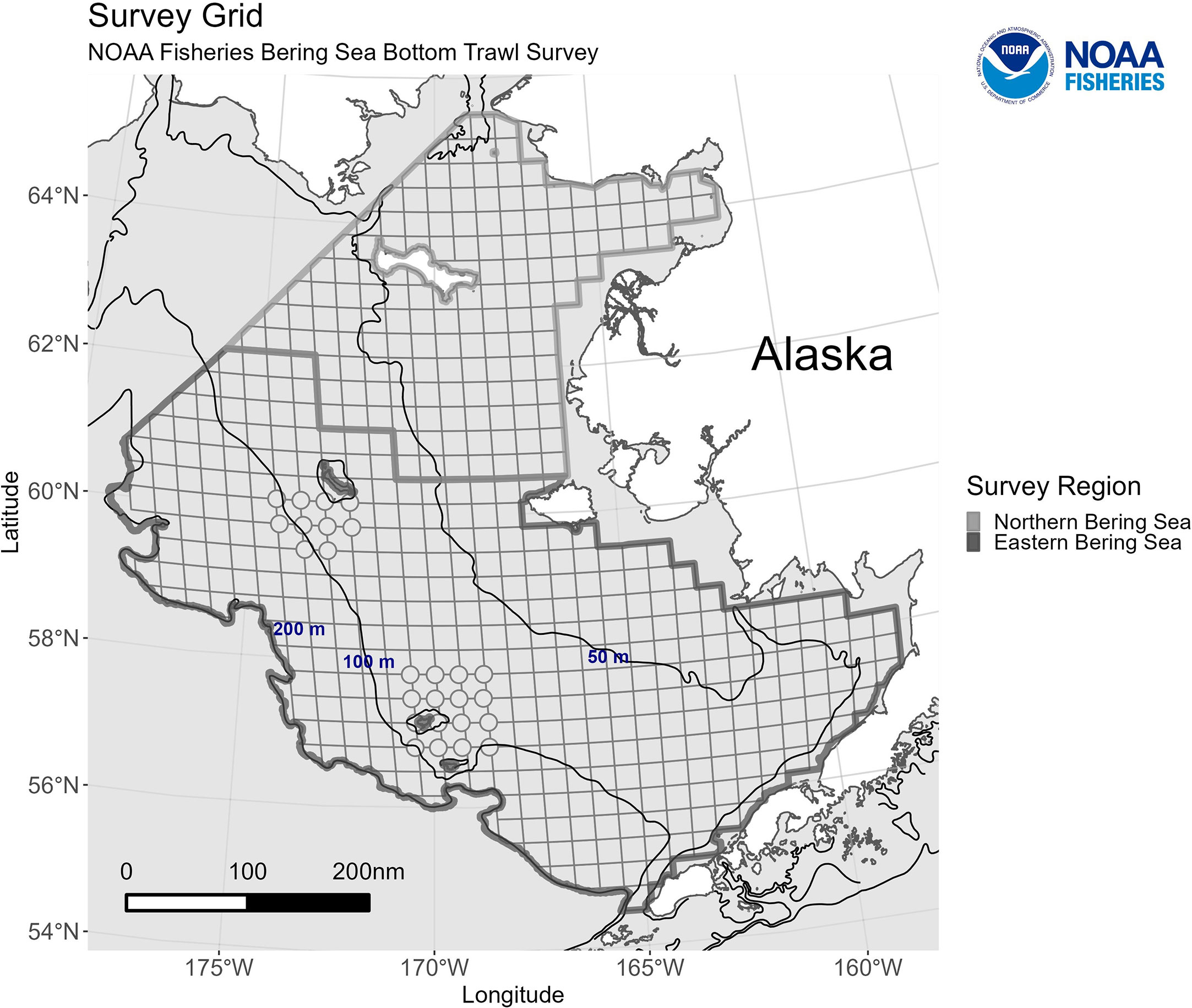
Figure 1 The Bering Sea bottom trawl survey grid, including the eastern Bering Sea standard survey area and the extension in the northern Bering Sea. Each square and circle (corner station) represents a survey station grid cell. The 50m, 100m, and 200m bathymetry lines are included for reference. https://www.fisheries.noaa.gov/alaska/science-data/near-real-time-temperatures-bering-sea-bottom-trawl-survey-2023

The EBS BTS also collects important oceanographic data used to develop environmental indices that help to explain species distributions (Stevenson and Lauth, 2019). One such index is the cold pool index (CPI). The CPI is an annual index derived from bottom temperature measurements taken at each survey station and measures the spatial extent (km²) of the cold pool. The cold pool is defined by bottom temperatures in the Bering Sea that are < 2°C (Wyllie-Echeverria and Wooster, 1998). This dynamic feature of the EBS is largely determined by annual sea ice coverage that regulates bottom temperature. Sea ice retreat in late winter/early spring leads to a small cold pool with bottom temperatures > 2°C. Conversely, later sea ice retreat maintains bottom temperature below 2°C and results in a larger cold pool. Species distributional changes with northward movement linked to the cold pool extent for some species in the Bering Sea have been predicted and documented (Stabeno et al., 2012; Stevenson and Lauth, 2019).

Model-based indices using the vector autoregressive spatio-temporal (VAST) model have been developed for walleye pollock and Pacific cod to combine the data from the standard EBS survey and the NBS extension (Thompson and Thorson, 2019; O’Leary et al., 2020). The CPI was included as a habitat covariate in the model to account for its impact on the distribution of these species over time. It is therefore imperative that we evaluate how well a spatio-temporal model can estimate abundance in a climate adaptive survey area, like the NBS extension, in years when not surveyed. Additionally, given the shifts in species distributions the expansion of the EBS BTS to the NBS needs to be conducted more frequently. An understanding of the required frequency and intensity of sampling is of utmost importance, so that survey resources can be allocated efficiently and effectively.

2.2 Empirical analysis

We conducted an empirical analysis to evaluate how well a spatio-temporal model can estimate biomass in a new or infrequently surveyed spatial stratum. We obtained and used EBS BTS catch rate data for four species of interest; walleye pollock, Pacific cod, yellowfin sole (Limanda aspera), and snow crab. All are among the most commercially important species in this region. They also exhibit different spatial distributions, where walleye pollock and Pacific cod have more widespread distributions, yellowfin sole is generally concentrated in the eastern portion of the EBS, and snow crab are predominately in the northwest. The full dataset (14,089 samples at approximately 376 unique stations) was reduced by dropping survey stations from one of four large areas in the EBS that were designed to mimic a circumstance where survey data were periodically unavailable in the eastern, northern, southern, or western portion of the full survey extent (Figure 2). The number of sampled stations retained was 11,399, 12,322, 10,367, and 11,357 when the eastern, western, northern, and southern stations were removed, respectively. We adopted the NBS sampling frequency, when the stations were dropped in all years of the time series except for those when the NBS was surveyed (i.e., keeping data across the full survey area only in 1982/1985/1988/1991/2010 and 2017-2019). This was done to mimic the unbalanced survey design of the NBS extension. The reduced dataset was then fitted to a spatio-temporal model developed in VAST (Thorson, 2019b) within R to estimate biomass indices for each species (Thorson and Barnett, 2017). The biomass indices from the full and reduced data sets were then compared.

FIGURE 2

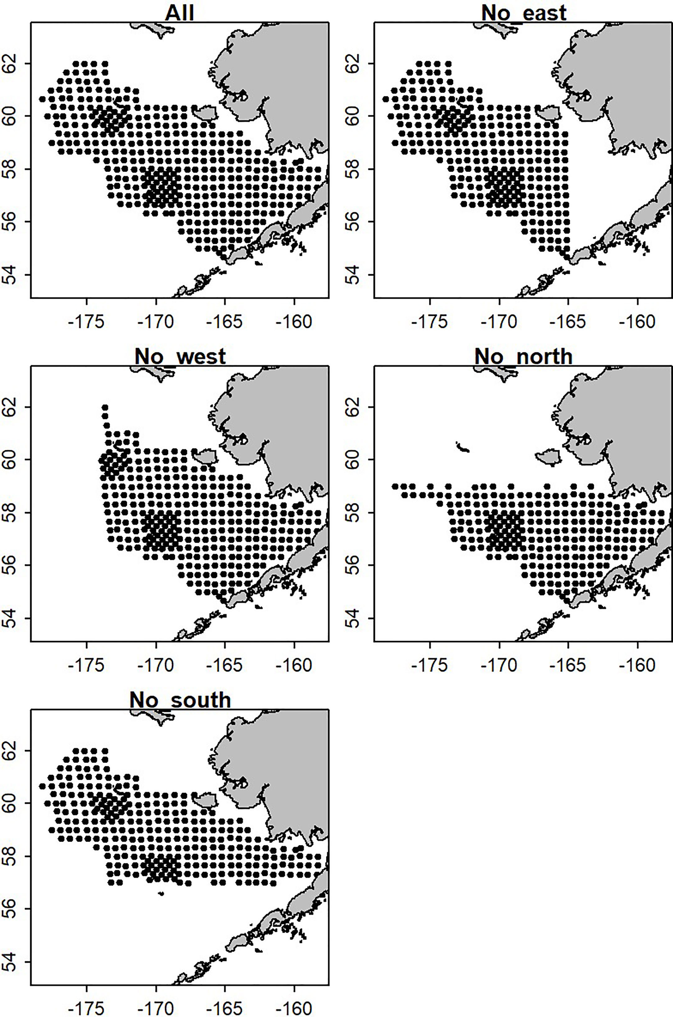
Figure 2 The survey footprint of the eastern Bering Sea bottom trawl survey standard area and four scenarios where data were removed from large areas.

The spatio-temporal model used for this analysis followed the guidelines in (Thorson, 2019b) and accounted for cold-pool effects. Biomass per unit area observations, b_i, from all EBS BTS grid cells for 1982-2019 were fit using a Poisson-link delta-gamma distribution. We wanted to estimate biomass in large unsampled areas in some years; therefore, the extrapolation to these areas was informed by estimating a zero-centered spatially varying coefficient (SVC) that measures the local response to an annual index of cold-pool extent index (Thorson, 2019b; Thorson et al., 2023). The SVC was estimated for both the linear predictors of the delta model. The variance of the SVC to cold-pool extent was estimated at zero for the second linear predictor of the yellowfin sole model. Therefore, it was removed from the yellowfin sole model for all scenarios. The two linear predictors of the delta model represent the encounter probability, p_i, and positive biomass per unit area, r_i.

The probability distribution of biomass sample b_i was specified as:

$$\text{Pr}(b_i>0)=1-p_i$$

and

$$b_i|B>0 \sim \text{Gamma}(B; {\theta }_b^{-2},r_i{\theta }_b^2),$$

where we specified a gamma distribution for positive catch rates where $r_i$ is the mean and ${\theta }_b$ is the coefficient of variation and we use the shape-scale parameterization. We estimated geometric anisotropy (i.e., the tendency for correlations to decline more rapidly in certain cardinal directions) (Thorson et al., 2015), and a spatial and spatio-temporal term for both linear predictors was included in the model. We also used epsilon bias-correlation to correct for retransformation bias (Thorson and Kristensen, 2016).

The linear predictors for numbers density, n_i, and biomass per individual, w_i, were

$$\text{log}(n_i)={\beta }_n(t)+{\omega }_n(s)+{ϵ}_n(s,t)+{\gamma }_n(s)T(t)$$

and

$$\text{log}(w_i)={\beta }_w(t)+{\omega }_w(s)+{ϵ}_w(s,t)+{\gamma }_w(s)T(t),$$

where ω_n and ω_w represent the time-invariant spatial variation, ϵ_n(t) and ϵ_w(t) represent the time-varying spatial variation, β_n(t) and β_w(t) represent the annual intercepts which are treated as fixed effects, T(t) is the cold-pool index (CPI) in each year, and γ_n and γ_wrepresents the log-linear impact of the CPI which vary spatially. We treat spatial terms (ω_n and ω_w) and SVCs (γ_n and γ_w) as Gaussian Markov random fields (GMRFs) and estimate them as random effects while estimating their variance as fixed effects. Similarly, we estimate spatio-temporal terms (ϵ_n(t) and ϵ_w(t)) as GMRFs that follow a first-order autoregressive process, and estimate their variance and temporal autocorrelation as fixed effects. The spatial domain included 100 knots and 2000 extrapolation grid cells that define the value of Gaussian Markov random fields (GMRFs) at the location of those knots, and the value of GMRFs elsewhere is calculated via bilinear interpolation.

Linear predictors were then transformed to calculate encounter probability $p_i$ and positive catch rate $r_i$ following the Poisson-linked delta model:

$$p_i=1-e^{a_i{n}_i}$$

and

$\begin{array}{ll}{r}_i=\frac{a_i{n}_i}{p_i}{w}_i& \text{,}\end{array}$

where $a_i$ is the area swept for each sample (Thorson, 2018). The spatio-temporal terms were estimated following a first-order autoregressive process across years to better estimate density hotspots. The temporal intercepts were treated as fixed effects for each linear predictor and year. Treating the temporal intercepts as fixed effects reduces the correlation structure among years so that the estimates can be used for assessment purposes. Lastly, the SVC ${\gamma }_p(s)$ and ${\gamma }_r(s)$ were estimated and assumed independent for p_i and r_i.

2.3 Simulation experiment

We also conducted a simulation experiment to evaluate the impact of sampling intensity and frequency on our biomass estimates in a new climate adaptive area. The operating model made the same structural assumptions as the estimation model used in the empirical analysis. The main difference between the two is that the spatial extent of the survey-sampling grid included the EBS and NBS bottom trawl survey stations (Figure 3). The OM was conditioned on the EBS BTS standard survey (1982-2018) and the NBS 2017 data through an initial model fit. Given the inconsistent frequency and unbalanced design of the NBS extension, we used the location of bottom trawl survey data in the NBS in 2017 to define the location of NBS sampling in 1982-2016 and 2018 to enable the OM to simulate data in the NBS in all years. The CPI was used in the model as an annual habitat covariate while estimating a zero-centered SVC for both predictors. In each simulation replicate, we then simulated new values for all fixed and random effects from the joint precision matrix estimated when fitting to real world data. We then simulated new survey observations conditional upon these simulated values for fixed and random effects. Therefore, each simulation replicate for a given sampling scenario differs in terms of true underlying densities, as well as resulting simulated samples of those densities.

FIGURE 3

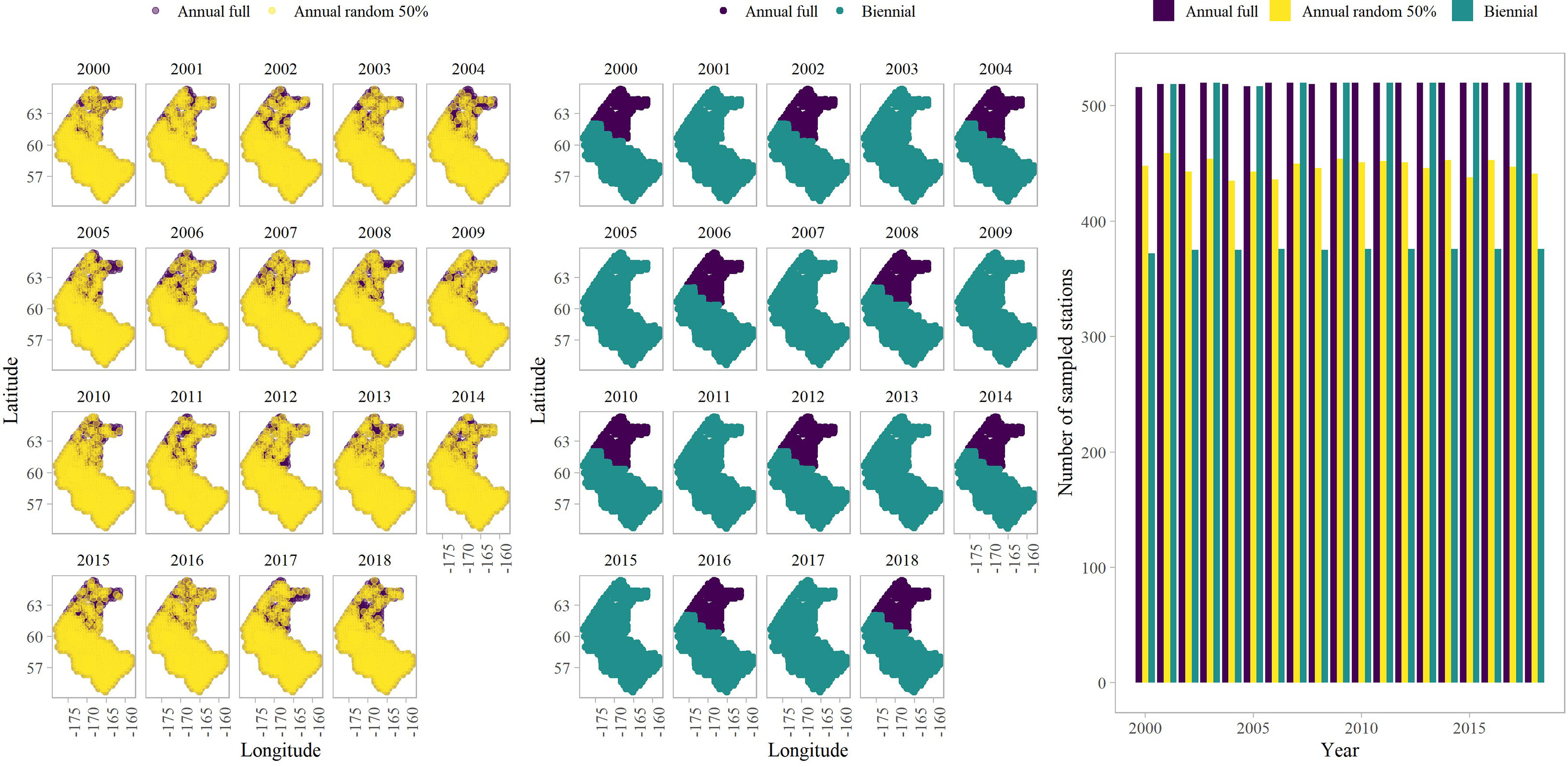
Figure 3 An example of the simulated sampling design scenarios: annual scenarios (left panel) and biennial scenario (middle panel), as well as the number of sampled stations per year (right panel).

The estimation model made the same structural assumptions as the OM; however, we reduced the number of knots to 50 from 250. Additionally, we subset the data to include the years 2000-2018. Using a subset of the data and reducing the number of knots reduced runtime. A total of 100 replicates were simulated for three survey sampling scenarios. The sampling scenarios included 1) annual and full sampling, 2) annual and full sampling in the EBS and a 50% reduction in survey stations while maintaining annual sampling in the NBS, and 3) annual and full sampling in the EBS and biennial sampling in the NBS, where odd years were sampled at all NBS stations. We randomly selected ~50% of NBS stations in scenario 2. We then evaluated performance by comparing the true proportion of biomass in the NBS in a given simulation replicate with the estimated proportion from each of three sampling scenarios. We specifically calculated bias on a log scale and the median absolute error in the proportion of biomass in the NBS to determine differences in the model estimation capabilities among the scenarios.

3 Results

3.1 Empirical analysis

Eliminating data from the eastern, western, northern, or southern portions for the majority of years and comparing results with those when using all data shows that the scale and trends in estimated biomass are generally similar for all four species (Figure 4). Removing data from large areas, thereby reducing the survey footprint, leads to greater uncertainty in the density estimates for all species and inaccuracy for some species. An interaction between species and the area removed was apparent, where greater uncertainty in the density estimates arose for particular areas for each species (e.g., comparing Figures 4, 5). For example, standard errors were larger when the west and north data were removed for walleye pollock, where they have tended to have increased density in years with low CPI (Figure 4, top row). Standard errors and inaccuracy were highest when the eastern data were removed for yellowfin sole (Figure 4, third row), which corresponds to core habitat for this species (Figure 5, third row; Table 1). Finally, removing the northern data resulted in the highest standard errors and inaccuracy for snow crab, which again corresponds to core habitat for snow crab (Figures 4, 5, bottom row; Table 1). The increased standard errors were similar across the removed areas for Pacific cod since this species has a more even distribution in the EBS than the other focal species (Figure 4, second row and where average density is similar across all scenarios in Table 1).

FIGURE 4

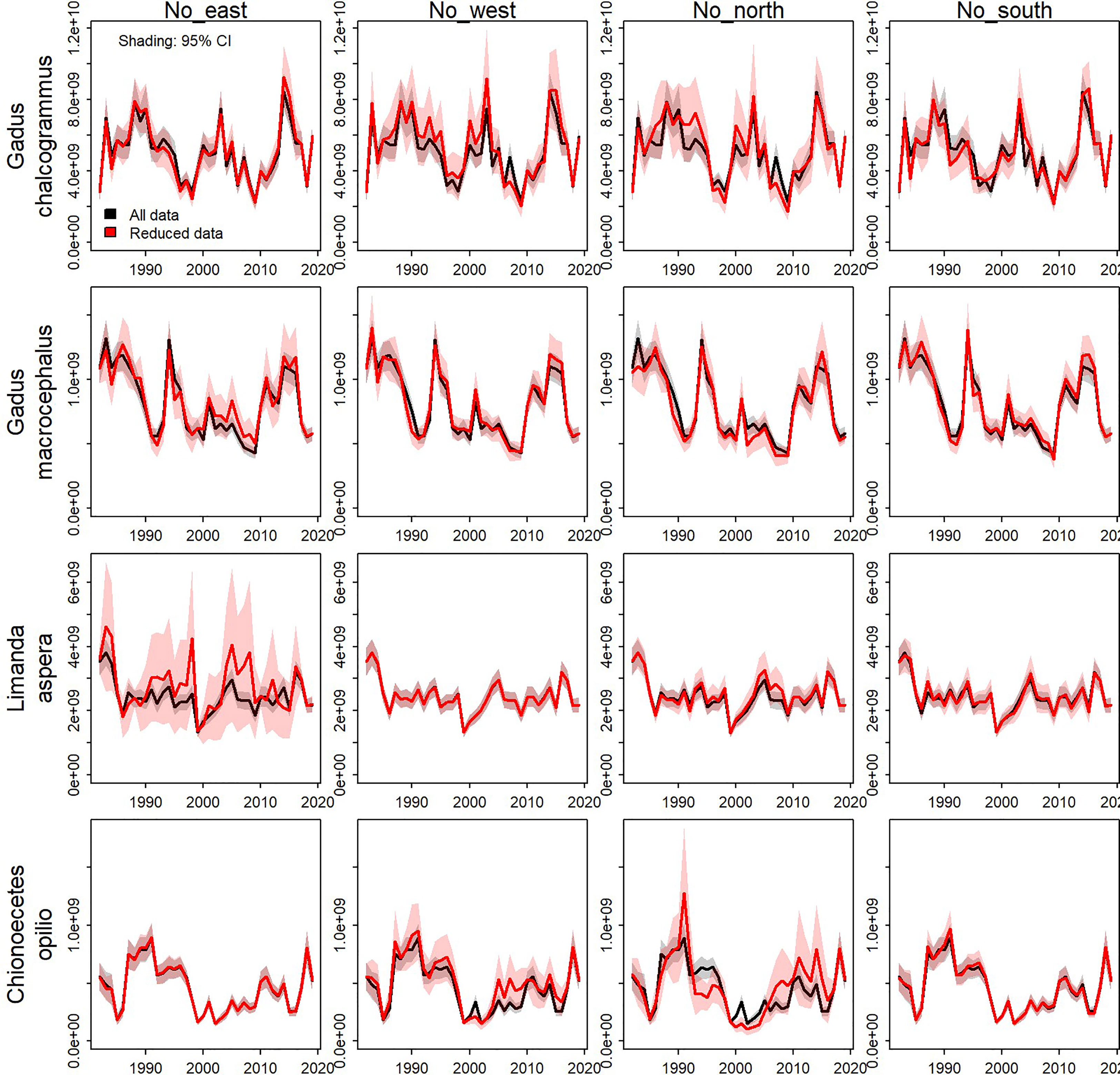
Figure 4 Biomass index estimates when the model was fit to all data (black line) and reduced data (red line) by species (rows) and areas removed from the data set (columns).Shaded regions represent the 95% confidence interval.

FIGURE 5

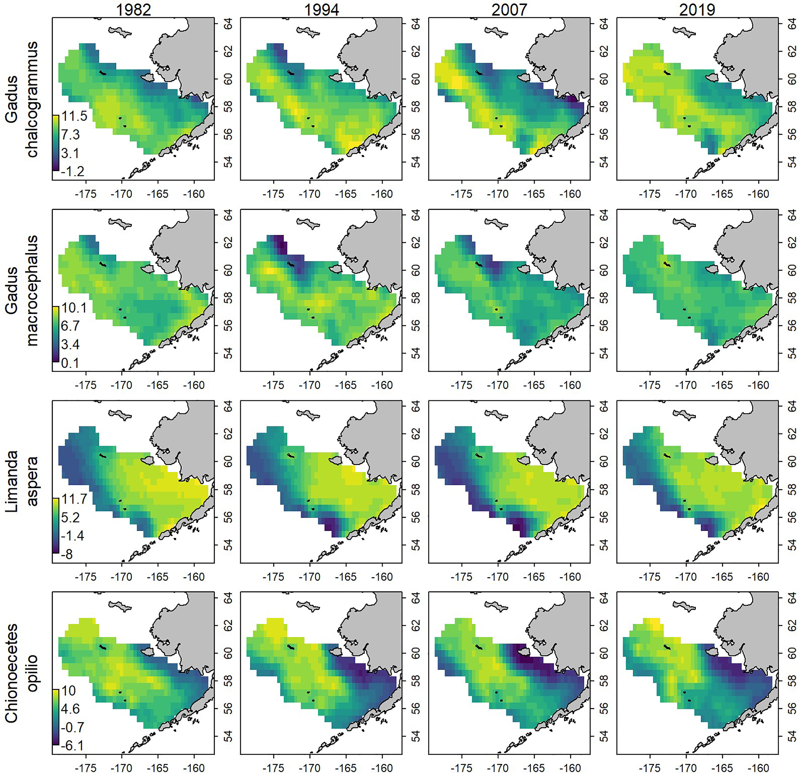
Figure 5 Estimate of log-biomass density, log_e(kg/km²), for evenly spaced years (columns) for each species (row) analyzed in the empirical analysis, estimated using the “full data set”. See Figure 2 for how these ranges overlap with the data-removal experiments.

TABLE 1

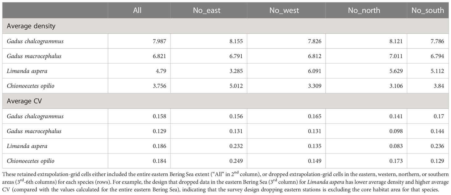
Table 1 The average (top rows) or coefficient of variation (bottom rows) for estimated density across years when fitting to all BT data in the eastern Bering Sea, computed at the set of extrapolation-grid cells that were retained across all years for a given sampling design.

3.2 Simulation experiment

We evaluated model convergence prior to processing the results and a total of 96, 87, and 96 model runs out of 100 converged for the annual, annual reduced, and biennial sampling scenarios, respectively. Of the model runs that converged, 82 simulations were in common among the scenarios. Greater bias was associated with biennial sampling than the annual sampling strategies (Figure 6). This was driven by the bias in the estimated proportion of biomass in years when the NBS was not surveyed (i.e., odd years). Bias in the biennial sampling was greater than the annual sampling strategies in the non-surveyed years, whereas the estimates were more similar among the sampling strategies when there was a temporal overlap in sampling. The biennial sampling strategy also exhibited greater uncertainty than the annual sampling strategies (Figure 6). The results are not unexpected given the total loss of information in the NBS in the even years.

FIGURE 6

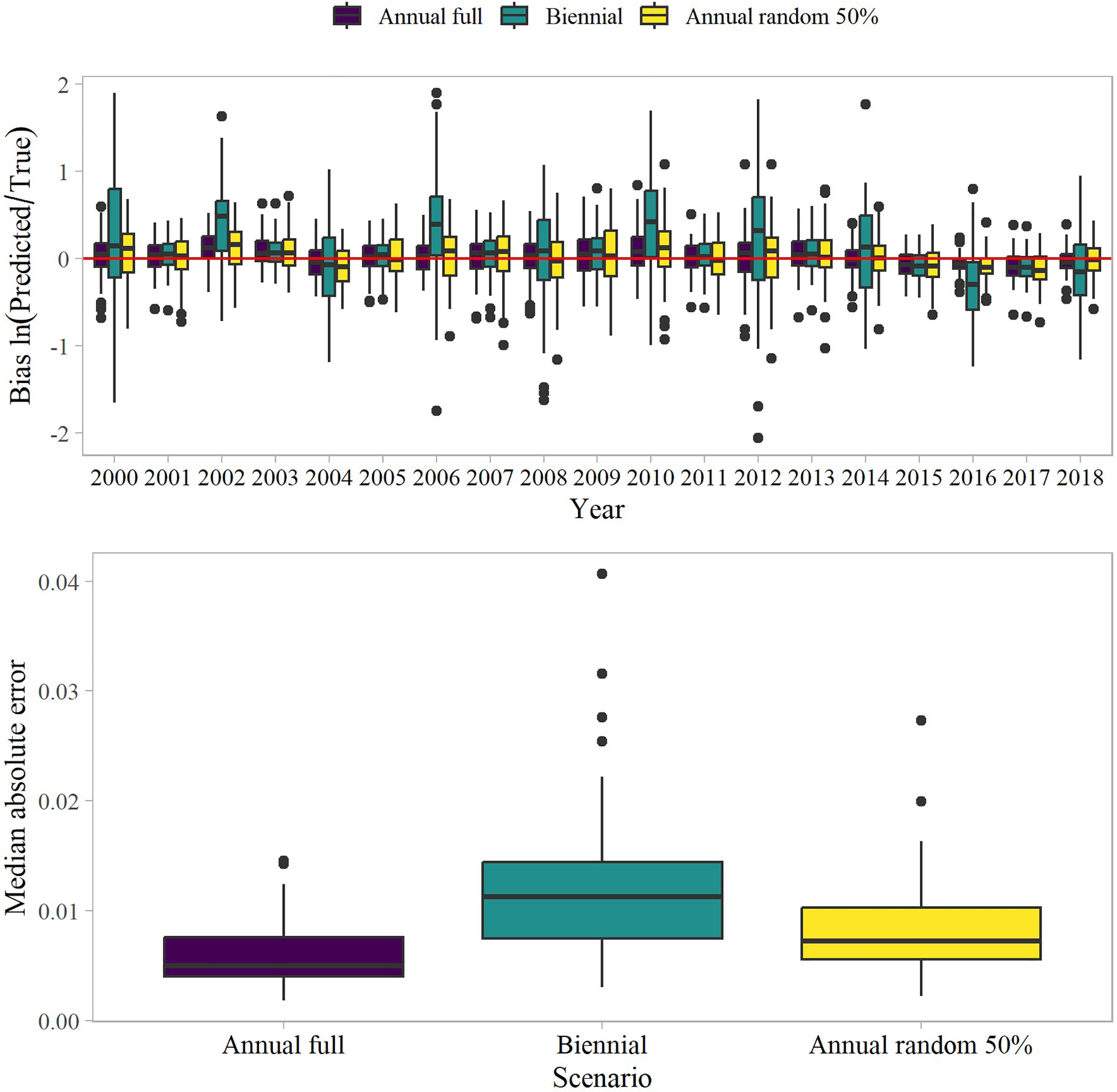
Figure 6 Bias in the estimated proportion of biomass in the northern Bering Sea for different sampling design scenarios (top panel) and the median absolute error among sampling scenarios (bottom panel). The boxplots are defined by the median (line), interquartile range (IQR, box), the furthest points from the 1.5 the IQR (whiskers), and outliers (points).

4 Discussion

Our study demonstrated that spatio-temporal models can successfully fill in data gaps in many circumstances when estimating abundance. Our empirical approach adopted the northern Bering Sea bottom trawl survey’s sampling frequency and removed observations from four large areas of the eastern Bering Sea standard survey area. We specifically showed that a spatio-temporal model using an environmental covariate (1) results in accurate biomass indices when the core of the stock’s range is not excluded from sampling, and (2) when the core of the stock’s range is excluded from data, the confidence intervals increase in width to still capture the abundance index that would arise using full data. We also used a simulation experiment to explore likely performance under alternative sampling strategies involving an infrequently surveyed area or a newer climate-adaptive survey area. The simulation experiment shows that the model has minimal bias and is precise when full sampling coverage is available in every year. However, if a reduction in sample sizes is necessary, reducing sampling density and maintaining annual sampling is more advantageous than maintaining sampling density at biennial sampling intervals. The overlap in the sampling and species spatial distributions, as well as survey frequency and intensity influenced the uncertainty estimates in our predictions. The benefits of adequate spatial coverage and annual sampling (i.e., reduced uncertainty in our biomass estimates) were obvious from our empirical and simulation experiments. For example, the better performance of the annual, reduced scenario in the simulation exercise indicates that having some information every year will improve annual estimates as opposed to have full information every other year. Spatio-temporal models, like VAST, rely on information from nearby locations and among years for extrapolation. It is therefore intuitive that excluding data from a large subarea that contains the center of a species distribution results in increased uncertainty. Similar results were shown for walleye pollock, where uncertainty estimates from a model similar to the one used in this study and using similar data was greater in years when the survey did not sample in the northern Bering Sea (O’Leary et al., 2020). Grüss and Thorson (2019) produced similar results to this study when simulating two scenarios: 1) the removal of the northwestern Gulf of Mexico (GOM) survey sample for red snapper (Lutjanus campechanus) and 2) not surveying the GOM over a number of early years. Uncertainty in their abundance estimates increased when either large spatial areas were not surveyed over time or a number of consecutive years were not sampled.

The uncertainty associated with survey biomass is an important stock assessment input, where estimates are calculated outside of the assessment and then inputted as the coefficient of variation (CV) into an assessment model. The CV value provides the model with a relative data weight associated with each observation and in relation to other sources of information. The data weights are used in the likelihood component of the assessment model and effectively determines how well the model will fit individual data points, as well as the entire time series (Francis, 2011). Stock assessment model outcomes can be highly sensitive to input data weights leading to greater uncertainty in estimates of current stock size and stock status and in the estimation of management reference points (Francis, 2011; Maunder et al., 2017; Punt, 2017). Hence, studies like the one presented here are important to conduct and ascertain how a change in survey sampling will affect the estimate of biomass and uncertainty.

Fishery-independent surveys collect a wide variety of data that go beyond biomass/abundance and include length and age composition data, as well as environmental data. Composition data provides information about changes in size and age structure, recruitment, growth, natural mortality, and in some cases sex ratio. Composition data are often included as proportions within a size or age class and the input sample size provides a measure of uncertainty. Biological (e.g., ontogenetic habitat, depth, and food preferences) and environmental drivers (e.g., bottom temperature) can lead to strong distribution patterns among lengths/ages within a species. Spatio-temporal models have been shown to effectively estimate compositional data and improve estimates of multinomial sample size (Thorson and Haltuch, 2019; O’Leary et al., 2020). This study focused on the impact of changing survey sampling on abundance estimates, but it is equally important to conduct a similar evaluation for composition data. A similar study should be conducted to determine the potential bias and uncertainty in the proportions at size/age and input sample size with changes in survey sampling. A loss of critical environmental data will be expected with changes in survey sampling. In the eastern Bering Sea the cold pool is an important oceanographic feature that is known to control species distribution in this region. Using an environmental index as a habitat covariate in a spatio-temporal model has been shown to be an effective way to model changes in species distributions and reduce uncertainty in abundance estimates (Thorson, 2019b; O’Leary et al., 2020). In our empirical analysis and simulations, we assumed that environmental data were available thereby we assumed we had perfect information about CPI. In reality, removing survey stations from a large area of the overall survey grid as was done for the empirical analysis would lead to a loss of information and affect our ability to calculate the CPI. In these cases, CPI could instead be calculated from other information, e.g., the Bering-10K Regional Ocean Modelling System which has been validated previously for this use (Kearney et al., 2021). Having an incomplete or alternative environmental index would lead to greater uncertainty in the model-based index. Therefore, our estimates may be optimistic and the loss of environmental information resulting from decreased sampling should be evaluated in the future.

The need to restructure sampling strategies will always be in the forefront for survey programs due to funding uncertainties, changes in species distributions and stock status, and the frequency of other unanticipated events like the COVID pandemic, or reduced or cancelled surveys due to inclement weather or a lack of funding. One certainty is that including biased inputs into a stock assessment will lead to biased results and management advice. Survey abundance is an assumed absolute measure or a relative measure and proportional to population biomass. The results from an assessment model will be impacted by the bias in the survey estimate and in turn lead to biased population estimates and management reference points. Therefore, obtaining unbiased survey estimates is integral to any assessment. The spatio-temporal model that we presented can provide unbiased estimates; however, it cannot ameliorate problems with non-representative sampling, as was demonstrated for yellowfin sole and snow crab when we excluded data from their core distributions. The empirical results also showed a non-uniform response among species and a trade-off among species and the removal of regional data. This has important implications on future surveys. As species distributions shift due to a changing climate, our surveys must adapt to effectively monitor variability and changing centers of distribution. The consequence of not doing so will likely be biased estimates; however, adaptability is no small task. Sampling optimization for all species within a multispecies fishery-independent survey is incredibly difficult. Spatio-temporal models and optimization methods should be used to identify trade-offs in bias/inaccuracy and uncertainty among species and strive to achieve representative sampling for as many species possible (Oyafuso et al., 2021).

Data availability statement

The raw data supporting the conclusions of this article will be made available by the authors, without undue reservation.

Author contributions

All authors conceived the ideas, designed methodology, and analyzed the data and were equally involved in manuscript writing. All authors contributed to the article and approved the submitted version.

Acknowledgments

We would like to thank the NOAA Alaska Fisheries Science Center (AFSC) Groundfish Assessment Program and their tremendous efforts during the eastern and northern Bering Sea shelf bottom trawl survey to collect the data and make it available for this analysis. We would also like to thank NOAA-AFSC reviewers Sandra Lowe and Drs. Steve Barbeaux and Zack Oyafuso for their valuable comments, as well as the journal reviewers.

Conflict of interest

The authors declare that the research was conducted in the absence of any commercial or financial relationships that could be construed as a potential conflict of interest.

Publisher’s note

All claims expressed in this article are solely those of the authors and do not necessarily represent those of their affiliated organizations, or those of the publisher, the editors and the reviewers. Any product that may be evaluated in this article, or claim that may be made by its manufacturer, is not guaranteed or endorsed by the publisher.

References

Bakkala R. G. (1993). Structure and historical changes in the groundfish complex of the eastern Bering Sea (United States Department of Commerce: NOAA Technical Memorandum NMFS 114), 86.

Google Scholar

Francis R. I. C. C. (2011). Data weighting in statistical fisheries stock assessment models. Can. J. Fish. Aquat. Sci. 68, 1124–1138. doi: 10.1139/f2011-025

CrossRef Full Text | Google Scholar

Grüss A., Thorson J. T. (2019). Developing spatio-temporal models using multiple data types for evaluating population trends and habitat usage. ICES J. Mar. Sci. 76, 1748–1761. doi: 10.1093/icesjms/fsz075

CrossRef Full Text | Google Scholar

ICES (2020). Workshop on unavoidable survey effort reduction (WKUSER) (No. 2:72), ICES scientific reports (Copenhagen: ICES).

Google Scholar

Kearney K. A., Alexander M., Aydin K., Cheng W., Hermann A. J., Hervieux G., et al. (2021). Seasonal predictability of sea ice and bottom temperature across the eastern Bering Sea shelf. J. Geophys. Res.: Ocean. 126, e2021JC017545. doi: 10.1029/2021JC017545

CrossRef Full Text | Google Scholar

Lo N. C., Jacobson L. D., Squire J. L. (1992). Indices of relative abundance from fish spotter data based on delta-lognormal models. Can. J. Fish. Aquat. Sci. 49, 2515–2526. doi: 10.1139/f92-278

CrossRef Full Text | Google Scholar

Markowitz E. H., Dawson E. J., Charriere N. E., Prohaska B. K., Rohan S. K., Stevenson D. E., et al. (2022). Results of the 2021 eastern and northern Bering Sea continental shelf bottom trawl survey of groundfish and invertebrate fauna (United States Department of Commerce: NOAA Technical Memorandum NMFS-AFSC-452), 215.

Google Scholar

Maunder M. N., Punt A. E. (2004). Standardizing catch and effort data: a review of recent approaches. Fish. Res. 70, 141–159. doi: 10.1016/j.fishres.2004.08.002

CrossRef Full Text | Google Scholar

Maunder M. N., Punt A. E., Valero J. L., Semmens B. X. (2017). Data conflict and weighting, likelihood functions and process error. Fisheries Research 192, 1–4. doi: 10.1016/j.fishres.2017.03.006

CrossRef Full Text | Google Scholar

Mueter F. J., Litzow M. A. (2008). Sea Ice retreat alters the biogeography of the Bering Sea continental shelf. Ecol. Appl. 18, 309–320. doi: 10.1890/07-0564.1

PubMed Abstract | CrossRef Full Text | Google Scholar

O’Leary C. A., DeFilippo L. B., Thorson J. T., Kotwicki S., Hoff G. R., Kulik V. V., et al. (2022). Understanding transboundary stocks’ availability by combining multiple fisheries-independent surveys and oceanographic conditions in spatiotemporal models. ICES J. Mar. Sci. 79, 1063–1074. doi: 10.1093/icesjms/fsac046

CrossRef Full Text | Google Scholar

O’Leary C. A., Thorson J. T., Ianelli J. N., Kotwicki S. (2020). Adapting to climate-driven distribution shifts using model-based indices and age composition from multiple surveys in the walleye pollock (Gadus chalcogrammus) stock assessment. Fish. Oceanog. 29, 541–557. doi: 10.1111/fog.12494

CrossRef Full Text | Google Scholar

Oyafuso Z. S., Barnett L. A. K., Kotwicki S. (2021). Incorporating spatiotemporal variability in multispecies survey design optimization addresses trade-offs in uncertainty. ICES J. Mar. Sci. 78, 1288–1300. doi: 10.1093/icesjms/fsab038

CrossRef Full Text | Google Scholar

Pecl G. T., Araujo M. B., Bell J. D., Blanchard J., Bonebrake T. C., et al. (2017). Biodiversity redistribution under climate change: impacts on ecosystems and human well being. Science 355, eaai9214. doi: 10.1126/science.aai9214

PubMed Abstract | CrossRef Full Text | Google Scholar

Perretti C. T., Thorson J. T. (2019). Spatio-temporal dynamics of summer flounder (Paralichthys dentatus) on the northeast US shelf. Fish. Res. 215, 62–68. doi: 10.1016/j.fishres.2019.03.006

CrossRef Full Text | Google Scholar

Pinsky M. L., Worm B., Fogarty M. J., Sarimiento J. L., Levin S. A. (2013). Marine taxa track local climate velocities. Science 341, 1239–1242. doi: 10.1126/science.1239352

PubMed Abstract | CrossRef Full Text | Google Scholar

Poloczanska E., Brown C., Sydeman W., Kiessling W., Schoeman D. S., Moore P. J. (2013). Global imprint of climate change on marine life. Nature Climate Change 3, 919–915. doi: 10.1038/nclimate1958

CrossRef Full Text | Google Scholar

Punt A. E. (2017). Some insights into data weighting in integrated stock assessments. Fish. Res. 192, 52–65. doi: 10.1016/j.fishres.2015.12.006

CrossRef Full Text | Google Scholar

Shelton A. O., Thorson J. T., Ward E. J., Feist B. E. (2014). Spatial semiparametric models improve estimates of species abundance and distribution. Can. J. Fish. Aquat. Sci. 71, 1655–1666. doi: 10.1139/cjfas-2013-0508

CrossRef Full Text | Google Scholar

Spies I., Gruenthal K. M., Drinan D. P., Hollowed A. B., Stevenson D. E., Tarpey C. M., et al. (2020). Genetic evidence of a northward range expansion in the eastern Bering Sea stock of pacific cod. Evolution. Appl. 13, 362–375. doi: 10.1111/eva.12874

CrossRef Full Text | Google Scholar

Stabeno P. J., Farley E. V. Jr., Kachel N. B., Moore S., Mordy C. W., Napp J. M., et al. (2012). A comparison of the physics of the northern and southern shelves of the eastern Bering Sea and some implications for the ecosystem. Deep-Sea Res. II 65–70, 14–30. doi: 10.1016/j.dsr2.2012.02.019

CrossRef Full Text | Google Scholar

Stauffer G. (2004). NOAA Protocols for groundfish bottom trawl surveys of the nation’s fishery resources (United States Department of Commerce: NOAA Technical Memorandum NMFS-F/SPO-65), 205.

Google Scholar

Stefansson G. (1996). Analysis of groundfish survey abundance data: combining the GLM and delta approaches. ICES J. Mar. Sci. 53, 577–588. doi: 10.1006/jmsc.1996.0079

CrossRef Full Text | Google Scholar

Stevenson D. E., Lauth R. R. (2019). Bottom trawl surveys in the northern Bering Sea indicate recent shifts in the distribution of marine species. Polar. Biol. 42, 407–421. doi: 10.1007/s00300-018-2431-1

CrossRef Full Text | Google Scholar

Thompson G. G., Thorson J. T. (2019). “Assessment of the pacific cod stock in the Eastern Bering Sea,” in Stock assessment and fishery evaluation report for the groundfish resources of the Bering Sea and Aleutian islands (605 W. 4th Avenue Suite 306, Anchorage: North Pacific Fishery Management Council).

Google Scholar

Thorson J. T. (2018). Three problems with the conventional delta-model for biomass sampling data, and a computationally efficient alternative. Can. J. Fish. Aquat. Sci. 75, 1369–1382. doi: 10.1139/cjfas-2017-0266

CrossRef Full Text | Google Scholar

Thorson J. T. (2019a). Measuring the impact of oceanographic indices on species distribution shifts: the spatially varying effect of cold-pool extent in the eastern Bering Sea. Limnol. Oceanog. 64, 2632–2645. doi: 10.1002/lno.11238

CrossRef Full Text | Google Scholar

Thorson J. T. (2019b). Guidance for decisions using the vector autoregressive spatio-temporal (VAST) package in stock, ecosystem, habitat and climate assessments. Fish. Res., 143–161. doi: 10.1016/j.fishres.2018.10.013

CrossRef Full Text | Google Scholar

Thorson J. T., Arimitsu M. L., Barnett L. A. K., Cheng W., Eisner L. B., Haynie A. C., et al. (2021). Forecasting community reassembly using climate-linked spatio-temporal ecosystem models. Ecography 44, 612–625. doi: 10.1111/ecog.05471

CrossRef Full Text | Google Scholar

Thorson J. T., Barnes C. L., Friedman S. T., Morano J. L., Siple M. C. (2023). Spatially varying coefficients can improve parsimony and descriptive power for species distribution models. Ecography 2023, e06510. doi: 10.1111/ecog.06510

CrossRef Full Text | Google Scholar

Thorson J. T., Barnett L. A. K. (2017). Comparing estimates of abundance trends and distribution shifts using single- and multispecies models of fishes and biogenic habitat. ICES J. Mar. Sci. 74, 1311–1321. doi: 10.1093/icesjms/fsw193

CrossRef Full Text | Google Scholar

Thorson J. T., Haltuch M. A. (2019). Spatiotemporal analysis of compositional data: increased precision and improved workflow using model-based inputs to stock assessment. Can. J. Fish. Aquat. Sci. 76, 401–414. doi: 10.1139/cjfas-2018-0015

CrossRef Full Text | Google Scholar

Thorson J. T., Kristensen K. (2016). Implementing a generic method for bias correction in statistical models using random effects, with spatial and population dynamics examples. Fish. Res. 175, 66–74. doi: 10.1016/j.fishres.2015.11.016

CrossRef Full Text | Google Scholar

Thorson J. T., Shelton A. O., Ward E. J., Skaug H. J. (2015). Geostatistical delta-generalized linear mixed models improve precision for estimated abundance indices for West coast groundfishes. ICES J. Mar. Sci. 72, 1297–1310. doi: 10.1093/icesjms/fsu243

CrossRef Full Text | Google Scholar

Thorson J. T., Ward E. J. (2013). Accounting for space–time interactions in index standardization models. Fish. Res. 147, 426–433. doi: 10.1016/j.fishres.2013.03.012

CrossRef Full Text | Google Scholar

Wyllie-Echeverria T., Wooster W. S. (1998). Year-to-year variations in Bering Sea ice cover and some consequences for fish distributions. Fish. Oceanog. 7, 159–170. doi: 10.1046/j.1365-2419.1998.00058.x

CrossRef Full Text | Google Scholar