 Elisabetta Canuti
- Joint Research Centre, European Commission, Ispra, Italy
Phytoplankton pigment data play a crucial role in ecological studies, enabling the identification of algal groups and estimation of primary production rates. Accurate measurements of chlorophyll a (TChl a) and other marine pigments are essential for the development of bio-optical algorithms and the validation of satellite data products. High-performance liquid chromatography (HPLC) is the gold standard method for quantifying multiple pigments in a single water sample. This study aims to investigate the uncertainties associated with phytoplankton pigment quantification by comparing duplicate sample analyses conducted by two laboratories, the Joint Research Centre of the European Commission (J) and the DHI Group, Denmark (D). The analyses were performed using the same HPLC method. The dataset comprised 957 natural samples collected between 2012 and 2017 from various European seas, representing different trophic conditions with TChl a concentrations ranging from 0.083 to 27.35 mg/m3. The study compared the results of the two independent analyses for TChl a and primary phytoplankton pigments, including chlorophyll b, chlorophyll c, carotens, fucoxanthin, 19′-butanoyloxyfucoxanthin, diadinoxanthin, diatoxanthin, 19′-hexanoyloxyfucoxanthin, peridin, and zeaxanthin. The percent difference between the two analyses was calculated to assess the uncertainties associated with pigment quantification. The mean percent difference observed between the two independent analyses of TChl a was 10.8%. For the primary phytoplankton pigments, the associated mean percent difference was 16.9%. These results meet the requirements of 15% and 25% uncertainties, respectively, which are applicable for the validation of satellite data products. The comparative analysis between the two laboratories demonstrates that the uncertainties associated with phytoplankton pigment quantification are within acceptable ranges for the validation of satellite data products. Moreover, the study investigates the propagation of uncertainties in diagnostic pigment values to phytoplankton indexes, which are derived using pigment-based algorithms to characterize phytoplankton populations according to functional types.
1 Introduction
The identification of phytoplankton pigments has a wide range of applications as chemotaxonomic markers to identify community composition (Jeffrey et al., 1997; Mackey, et al., 1996; Wright and Jeffrey, 2005; Roy et al., 2011), species and their biomass in seawater (Vidussi et al., 2001; Uitz et al., 2006; Hirata et al., 2011) and plays a role in the development, refinement, and validation of satellite algorithms for mapping phytoplankton biomass, functional types, and size classes (e.g., Brewin et al., 2010; Mouw et al., 2017).
Ocean color data validation, satellite bio-optical algorithm development, and ocean productivity models within the framework of marine ecosystem studies, also require high-quality in situ measurements of chlorophyll a (TChl a) and primary pigment concentrations. Validation of satellite products of TChl a is particularly relevant as it is listed as an essential climate variable (GCOS, 2011). The phytoplankton pigments of algae can be routinely quantified through liquid chromatographic screening methods to separate known pigments quantitatively. More than 30 high-performance liquid chromatography (HPLC) methods are reported in the literature (Roy et al., 2011) as commonly implemented for phytoplankton pigment determination. The HPLC methods primarily utilized for remote sensing validation activities are based on C8 and C18 chromatographic columns. In the JGOFS Protocols for the Joint Global Ocean Flux Study Core Measurements (1994), the Wright et al. (1991) method was recommended as the HPLC method for determining TChl a. In the oceanographic community, the Zapata et al. (2000) and Van Heukelem and Thomas (2001) methods have gained widespread adoption over the past decade. These two methods offer the advantage of enabling the simultaneous analysis of multiple pigments and unknowns in a single run (Wright and Jeffrey, 2005), while also exhibiting superior resolution for chlorophylls c compared to Wright’s approach (1991).
Moreover, to ensure a continuous high standard in sample analysis, regular participation in comparison exercises involving international laboratories or comparison with a certified reference laboratory are required. The so-called round-robin exercises have been conducted in the past decades to assess the performance of HPLC methods applied for pigment determination, and uncertainties of 15% have been documented for TChl a and other pigments (Latasa et al., 1996; Claustre et al., 2004). It is worth highlighting that the majority of studies tend to focus on TChl a analysis, while comparatively fewer investigations are dedicated to other pigments. This disparity is noteworthy as it limits our understanding of the broader spectrum of pigments present in various samples. Natural samples, such as those obtained from different marine environments, exhibit a diverse range of pigments with unique functional roles. Understanding the full pigment profile of natural samples requires comprehensive HPLC comparisons that encompass not only TChl a but also other pigments such as chlorophyll b, carotenoids, and phycobilins. The SeaWiFS HPLC Analysis Round-Robin Experiment (SH) and the HPLC/DAD Intercomparison on Phytoplankton Pigments (HIP) exercises have compared laboratories on several pigments, relying on both pigment standard and natural samples in their statistics. Such exercises have the great merit of allowing the comparison of methods and performance among the participating institutes, typically 4 to 11 (Table 1) on different water types. In SH and HIP exercises (with the exception of HIP-3), a quality assurance (QA) subset of laboratories was defined that represented the state-of-the-art results based on agreed parameters of performance metrics (Hooker et al., 2005). The TChl a average uncertainties for the QA subset were invariant to water type and lower than 8%, while a result lower than 25% for primary pigments was reached in all the exercise with the exception of SH-4, which was focused on eutrophic waters (Hooker et al., 2010). Although the level of agreement requested for remote sensing applications is demonstrated to be achievable, some participants not part of the QA have shown differences much higher than 15% for the TChl a, and than 25% on average on primary pigments (Hooker et al., 2005; Hooker et al., 2009; Hooker et al., 2010; Hooker et al., 2012; Canuti et al., 2016; Canuti et al., 2022). A known limit of the comparison of marine pigments is the lack of certified reference materials (CRMs); instead, pigment standards certified by analysis from a select few producers (e.g., DHI, DK, and carotenature, CH) were commonly used.
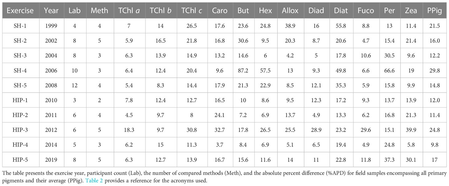
Table 1 Overview of the outcomes from the initial five HIP comparison exercises and the five SeaHARRE (SH) trials.
The current study first aims to investigate the uncertainties associated with phytoplankton pigment quantification by comparing the analyses performed on duplicate samples by a certified laboratory and an accredited laboratory applying the same method (Van Heukelem and Thomas, 2001): the Joint Research Centre of the European Commission (J) and the DHI Group, Denmark (D). The comparison with one accredited laboratory allows for a focused examination of the same method applied to various water types and is significant as both laboratories have shown good performance in previous intercomparison exercises (e.g., Canuti et al., 2016). The chromatographic method selected here has been successfully applied to a wide range of pigment concentrations, including oligotrophic (Hooker et al., 2009) and eutrophic coastal waters (Hooker et al., 2005). However, the most relevant aspect of the study is the data set available for analysis, made up of batches of natural samples collected at 957 measurement stations during ship-based oceanographic campaigns and analyzed by both laboratories. These data are representative of different trophic conditions and water types of the European Seas, with TChl a concentration in the range of 0.083–27.35 mg/m3, allowing an extensive comparison to be conducted. The phytoplankton pigments considered for the present exercise are the chlorophylls and the carotenoids most commonly used in marine chemotaxonomic and photo-physiological studies, including the major marker pigments used for classification of phytoplankton groups in ecological studies (Roy et al., 2011). Phytoplankton pigment datasets are commonly used to characterize algal species in terms of phytoplankton functional types (PFTs) or phytoplankton size classes (PSCs). Related investigations have been pursued in the context of ocean color remote sensing, as this would allow a synoptic description of PFTs or PSCs (e.g., IOCCG, 2014; Mouw et al., 2017; Xi et al., 2020). The two most widely used PFT methods are CHEMTAX (Mackey et al., 1996) and diagnostic pigment (DP) analyses. The a priori assumption underlying the chemotaxonomy methods is the covariance of pigments. The inherent uncertainties of chemotaxonomy methods are due to the widespread occurrence of most pigments across many different taxa (IOCCG, 2014). Another known limit is the association of a single pigment with a taxon even though it could be, in some case, not representative of the entire group, e.g., some Dinoflagellates spp. have types of “non-canonical” plastids instead of the Peridinin (Matsumoto et al., 2011), and there are known cases (Naik et al., 2011) where the chemotaxonomy alone leads to incomplete interpretation of the taxa distribution. Despite these considerations, most of the validation of remote sensing methods for assessing phytoplankton community composition is based on chemotaxonomy derived from HPLC pigments. Tracing uncertainties and building uncertainty budgets for descriptors of phytoplankton populations are tasks in progress (Bracher et al., 2017), where uncertainties associated with field data of diagnostic pigments are needed (Xi et al., 2021). The present study obviously contributes to that effort. A second contribution is to explore how uncertainties in diagnostic pigment values propagate to phytoplankton indexes that are at the basis of pigment-based algorithms deriving descriptors of phytoplankton populations such as PFTs (Hirata et al., 2011), therefore providing a benchmark value for that step.
2 Materials and methods
2.1 Nomenclature and use of diagnostic pigments
The nomenclature adopted for total chlorophylls and the other pigments is the one established by the Scientific Committee on Oceanographic Research (SCOR) Working Group 78 (Jeffrey et al., 1997). The individual pigments could be used to obtain the pigment associations and to derive macrovariables such as sums, ratios, and indices (Table 2).
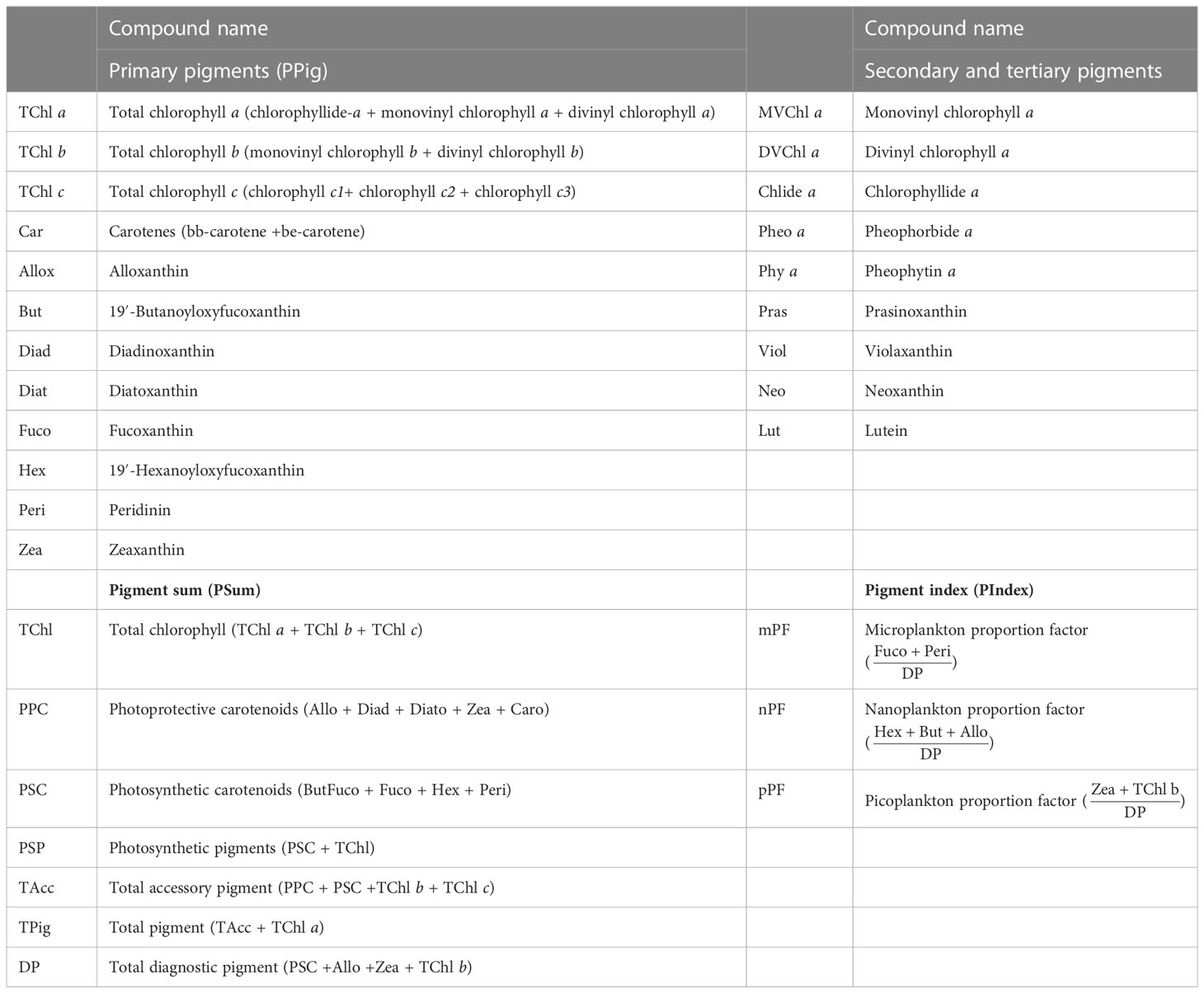
Table 2 Individual pigments and pigment associations to derive macrovariables as sums, ratios, and indices and their acronyms.
Vidussi et al. (2001) introduced a method that established a connection between diagnostic accessory pigments (peridinin, 19′-butanoyloxyfucoxanthin, fucoxanthin, 19′-hexanoyloxyfucoxanthin, alloxanthin, chlorophyll b, and zeaxanthin) and various taxonomic groups of phytoplankton, enabling the derivation of PFTs across three distinct size classes. These size classes encompassed micro- (> 20 µm), nano- (2–20 µm), and picoplankton (0.2–2 µm), representing a comprehensive range of trophic conditions and taxonomic classes, including diatoms, dinophytes, cryptophytes, haptophytes, green algae, and prokaryotes (Tables 2, 3). Building upon this foundation, Uitz et al. (2006) further refined the methodology by incorporating weighting coefficients for the same set of seven diagnostic pigments. This algorithm required the quantification of DPs using HPLC. These DPs formed a minimal set of marker pigments capable of detecting the primary phytoplankton types (as outlined in Table 3). The determination of PFTs relied on estimating the abundance of each phytoplankton group based on the established relationship between TChl a and their respective quantities (Uitz et al., 2006; Brewin et al., 2010; Hirata et al., 2011). In this work, we apply the known relationships between pigment abundances without any additional adjustments to the coefficients, adhering to the methodology outlined by previous studies.
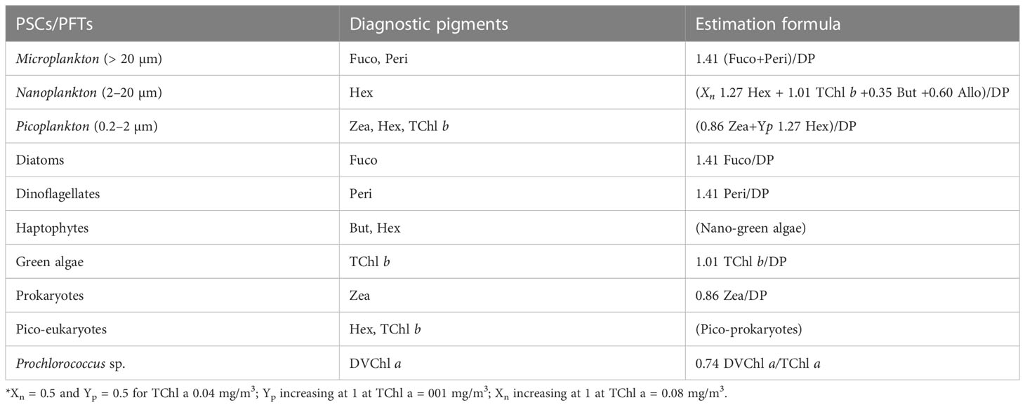
Table 3 Phytoplankton size classes (PSCs), phytoplankton functional types (PFTs), diagnostic pigments, and their taxonomic meaning.
Xn indicates a portion of nanoplankton contributing to Hex, and Yp indicates a portion of picoplankton in Hex (Brewin et al., 2010)
2.2 Sampling
The duplicate natural samples used to support the investigation were collected by the Joint Research Centre (JRC) between 2012 and 2017 across the European Seas during 11 different oceanographic cruises in the framework of the Bio-Optical Mapping of Marine Properties (BiOMaP, Zibordi et al., 2011) program and 26 measuring campaigns at the Acqua Alta Oceanographic Tower (AAOT) located in the Gulf of Venice, Italy, northern Adriatic Sea (45.31° N, 12.51° E). To minimize the intraseries variability due to different operators and filtering procedures, a common standard operative procedure was adopted. The water batch for replicate production was collected using Niskin or Plexiglas sampling bottles. In the case of a surface batch, the water was collected 1 m below the surface. Samples were collected at the surface for all the ship-based campaigns and at the additional depths of 8 and 14 m during the AAOT measurement campaigns. The water batch was filtered through a polyethylene (PE) mesh size of 300 µm (Kartell, Milan, Italy) and collected in a 10-L polypropylene (PP) bottle. The water was kept well mixed. The filtration volumes were evenly distributed among two cylinders previously rinsed. The filters used for the comparison were 25 mm GF/F (nominal pore size, 0.7 µm). The two filtrations were conducted in parallel under a mild vacuum (not exceeding 0.5 atm). At the end of the water passage, a few extra seconds of vacuum were applied to dry the filter before storage. The filters were then folded in two parts with the filtrate inside, wrapped in aluminum foil, flash frozen in liquid nitrogen, and stored until their arrival at the JRC Marine Optical Laboratory. The samples were successively moved to a −80°C freezer (ThermoFisher, USA) until shipped in dry ice (−40°C) to the D, where the laboratory analysis was performed. The water volume filtered varied from 60 ml (N02 cruise) to 2,000 ml (I02 cruise) and was established according to the water absorption coefficient measured in situ by an ac-9 meter (WET Labs Inc., USA) at 412 nm. The complete list of natural samples and their locations are summarized in Table 4 and displayed in Figure 1.
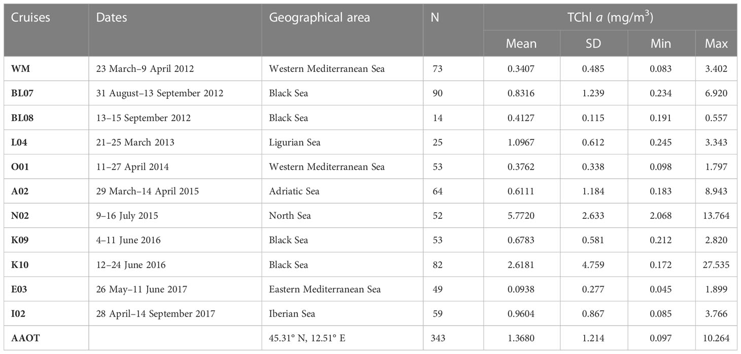
Table 4 Overview of the HPLC pigment database categorized by cruise, date, geographical area, and number of stations (N).
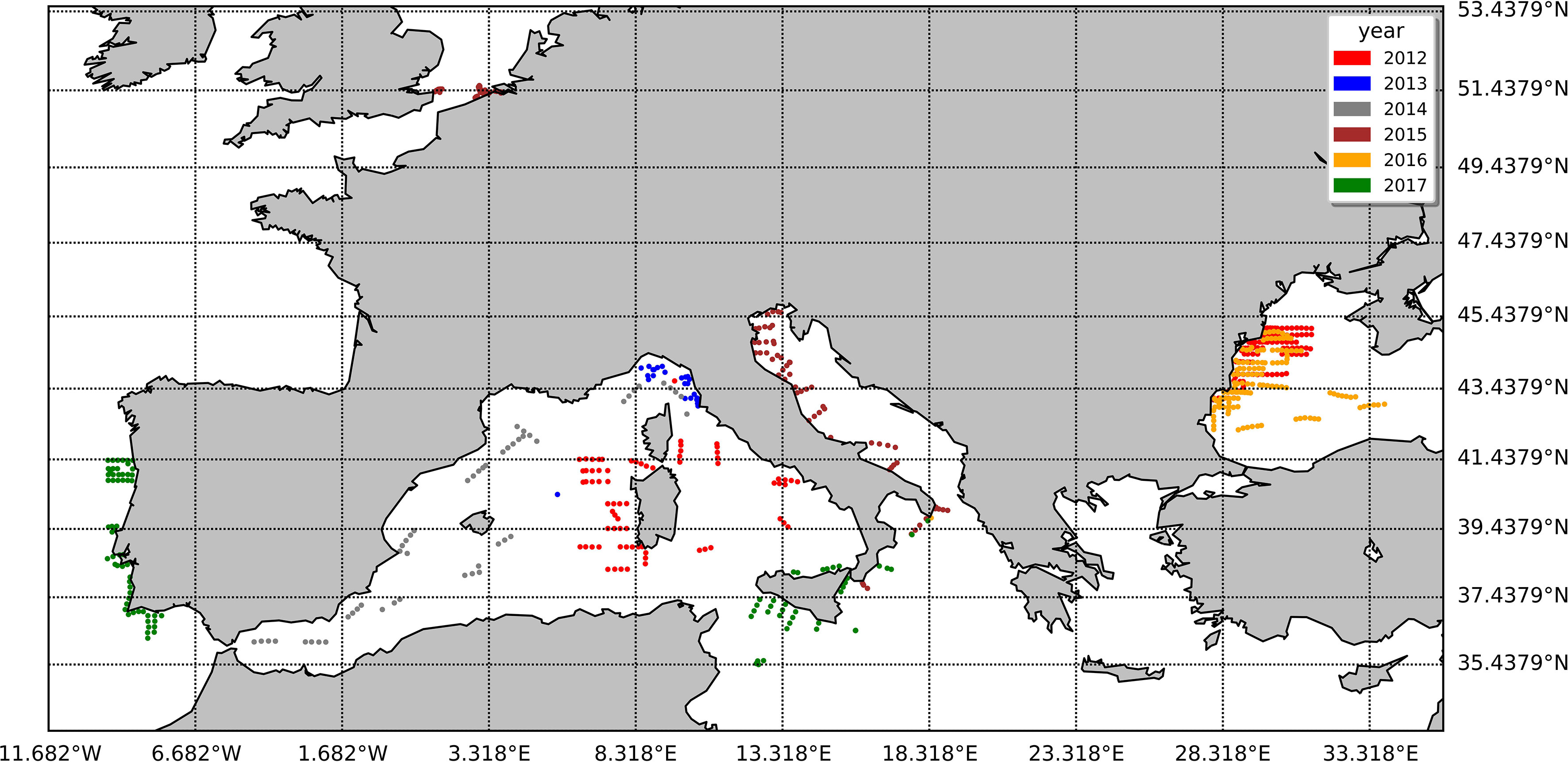
Figure 1 The spatial arrangement of the natural samples utilized in this study, with distinct colors representing various years.
The datasets considered in the following analysis refer to 957 samples: 614 belonging to oceanographic cruises and approximately one third (343 samples) collected at AAOT.
The table provides information on surface TChl a range (min and max), average concentration (mean), and standard deviation (SD) for all campaigns, except for the AAOT campaign, where the TChl a data pertain to all depth samples collected at the specific site.
2.3 Analytical method
The quantitative HPLC method applied by the two laboratories for the determination of phytoplankton pigments is the Van Heukelem and Thomas (2001) method. However, the single laboratory implementation could differ from the method originally published.
The D method is described in detail in Schlüter et al. (2016). The main information reported here is that described by D in the test reports delivered together with the results of accredited pigment analysis and have to be considered the conditions of analysis for the accredited method (DHI Internal Method SOP No. 30/852:05). The filters are transferred to vials with 3 ml of 95% acetone with an internal standard (vitamin E). The samples are mixed on a vortex mixer, sonicated in an ice-cold sonication bath for 10 min, extracted at 4°C for 20 h, and mixed again. The samples are then filtered through a 0.2-μm Teflon syringe filter into HPLC vials and placed in the cooling rack of the HPLC system together with the vials with mixed pigments. The samples were analyzed by a Shimadzu LC-10ADVP HPLC composed of one pump (LC-10ADVP), a photodiode array detector (SPD-M10AVP), an SCL-10ADVP system controller with LC Solution software, a temperature-controlled auto sampler (set at 4°C), a column oven (CTO-10ASVP), and a degasser. A buffer consisting of 28 mM aqueous tetrabutylammoniumacetate (TBAA) and the sample are injected in the HPLC in the ratio 5:2 using a pretreatment program and mixing in the loop before injection, for a total of 500 µl. The solvents used are methanol and 28 mM aqueous TBAA. The solvent gradient, with a constant flow of 1.1 ml/min consists of solvent A ((70:30) methanol:28 mM aqueous TBAA, pH 6.4) and solvent B (100% methanol). The time gradient program was at 0 min: 95% A, 5% B; 22 min: 5% A, 95% B; 30 min: 95% A, 5% B; 31 min: 100% A, 0% B; 34 min: 100% A, 0% B; 35 min 5% A, 95% B; and 41 min: stop. The column was an Eclipse XDB-C8, 3.5 μm particle size, 150 × 4.6 Φ mm (Agilent Technologies, Santa Clara, California, USA). The temperature of the column oven was set to 60°C. The HPLC was calibrated with pigment standards from DHI Lab Products, Denmark. The internal standard was detected at 222 nm, while the rest of the pigments were detected and identified by online PDA analysis at 450 nm. The derived pigment concentrations of each sample are provided through Excel sheets. As declared in the D Test Reports, “the precision of the HPLC method is approximately 1%.” Chl c1 is partly co-eluted with Chl c2. Still, their peaks are separated by the HPLC software, and Chl c1 is calculated by the response factor (RF) of Chl c2.
The J method is described in detail in Hooker et al. (2010). The samples are cut in pieces into a 10-ml polypropylene plastic tube (Corning Inc., Arizona, USA) with 2.5 ml of 0.025 g/L of internal standard (α-tocopherol, Honeywell, North Carolina, USA) dissolved in acetone (HPLC gradient, Merck, Darmstadt, Germany) and 150 μl of MilliQ water, and soaked for 1 h at −20°C. They are successively sonicated for 90 s in ice with a sonication probe (BANDELIN electronic, Berlin, Germany). The samples are then soaked for 3.5–4 h at −20°C, extracted through a 0.2-μm Teflon syringe filter into an amber vial, mixed by vortex, and transferred into a HPLC vial. Samples are preserved at 4°C in the thermostated auto sampler until the analysis is performed. The samples were analyzed by a 1200 Agilent Tech HPLC composed of a degasser (G1379A), a quaternary pump (G1311A), a photodiode array detector (G1315D), a temperature-controlled auto sampler (G1329A) set at 4°C, a column oven (G1316A) set at 60°C, and a system controller with Open LAB CDS control software. The column was an Eclipse Zorbax Eclipse XDB-C8, 3.5 μm particle size, 150 × 4.6 Φ mm (Agilent Technologies, Santa Clara, California, USA). The sample is mixed in a 900-µl preinjection loop with a buffer consisting of 28 mM aqueous TBAA (150 µl sample +375 µl buffer) before the injection into the HPLC. With respect to the original method, the solvent gradient consisted of three solvents: solvent A ((70:30) methanol:28 mM aqueous TBAA, pH 6.5), solvent B (100% methanol), and solvent C (100% acetone). All the solvents are suitable for chromatographic analysis. The acetone was flowed for 1 min at the end of each sample to avoid a carry-over to the next analysis The flow rate was 1.1 ml/min except when the solvent C was added (flow rate = 1.3 ml/min). The time program was at 0 min: 95% A, 5% B; 22 min: 5% A, 95% B; 24.5 min: 5% A, 95% B; 24.75 min: 5% A, 65% B, 30% C; 25.75 min: 5% A, 65% B; 30% C (flow 1.3 ml/min); 25.85 min: 5% A, 65% B, 30% C 100%; 26.10 min 95% A, 5% B; and 32 min: stop. The HPLC was calibrated with pigment standards (DHI Lab Products, Denmark). The calibration curve consisted of nine points covering from a dilution close to three times the signal-to-noise ratio (SNR) concentration to the standard concentration (Hooker et al., 2005). The calibration curves were checked for linearity in the full analysis range. The low-limit of detection (LOD) is assumed to be three times the instrumental SNR at each quantification wavelength. Peaks below the LOD are considered not identified. The internal standard was detected at 222 nm; MV Chl a, DVChl a, Chlide a, Pheo a, Phy a were detected at 665 nm; all other pigments were detected at 450 nm. Chl c1 is quantified using the RF of Chl c2, and the DVChl b is quantified using the RF of MVChl b.
The extraction procedure constitutes the main difference between the two methods (see Table 5 for details): D soaks the samples for 20–24 h and uses a sonication bath for sample disruption. Conversely, J soaks the sample for 3.5–4 h and uses a sonication probe for sample disruption. It is expected that the different extraction time does not affect the quantification of pigments (Wasmund et al., 2006). In addition, the chromatographic methods (Table 5) differ by minor adjustments of the mobile phase gradient (i.e., the acetone rinse for J and a total analysis time of 32 min for J and 41 min for D).
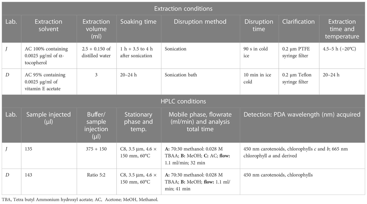
Table 5 A summary of sample extraction for Φ 25 mm GF/F (0.7 µm pore size) and HPLC conditions for J and D: injection, mobile and stationary phases and detector acquisition settings.
The pigment concentrations () are calculated by each laboratory as:
where is the pigment concentration as obtained from HPLC, is the extraction volume, is the volume of the water filtered for each sample, and is the amount of sample injected into the column.
2.4 Quality assurance and laboratory performance
The J is Quality Standard ISO 9001 certified, while the D is DANAK quality accredited (ISO/IEC 17025:2005) for phytoplankton analysis. D and J both participated in the SeaWiFS HPLC Analysis Round-Robin Experiment (SeaHARRE-4, Hooker et al., 2010) and the HPLC Intercomparisons on Phytoplankton Pigments (HIP-1 and HIP-4, Canuti et al., 2016). During these comparison exercises, the laboratory uncertainties on standard and on natural samples were assessed following a chemo-metrics criteria approach that has already been adopted in several HPLC intercomparison exercises on phytoplankton pigments (Claustre et al., 2004; Hooker et al., 2005; Hooker et al., 2009; Hooker et al., 2010 and Hooker et al., 2012; Canuti et al., 2016). Summary results for J and D in such exercises are provided here to give background on the expected performance of these laboratories.
The parameters considered are percent differences or variation coefficients of the quantities identified as being the most relevant to describe the quality of the chromatography analysis. In the present work, only an overview of the performance metrics calculation is given. In such intercomparison exercises, NS batches of samples are distributed to the participants, with each sample having typically two or three replicates. The true value of the concentration of each batch of samples is assumed to be the mean concentration of samples among participating laboratories or methods. For pigment p, the mean pigment concentration () for each sample series Sk is calculated as:
where i refers to the laboratory, is the average pigment concentration for pigment p over the replicates for sample Sk, and N is the number of participants.
The variation coefficient (CV), ξ, expressed as the percent ratio of the standard deviation, σ, in the replicates with respect to the average concentration of the replicates is a measure of the precision achieved for a sample:
ξ values are calculated for each pigment, sample, and participant, and the mean precision for a specific laboratory i and pigment p is obtained by averaging over the NS samples Sk:
An unbiased percent difference , or its modulus , is selected as an indicator of a method accuracy, with reference to the laboratory average :
Similarly to Eq. [4], the accuracy for laboratory i and pigment p is computed by taking the average of over the NS samples.
Using the results of the HIP-4 exercise conducted in 2011 (Canuti et al., 2016), the accuracy and precision on natural samples of primary pigments primary pigments (PPig) were, respectively, 4.7% and 6.4% for D and 5.5% and 7.4% for J, which ranks the methods used in the two laboratories as “quantitative methods” according to the SeaHARRE-2 quality scheme. Considering the low concentration range of most of the samples included in HIP-4 (< 1 mg/m3), an additional parameter of interest to assess the quality of the methods is the accuracy of the HPLC calibration curve, which was found to have an average value of 4.3% for J (corresponding to “quantitative” performance) and 0.9% for D (“state-of-art” performance).
The criteria established in Aiken et al. (2009) and used for assessing the quality of data sets used for bio-optical algorithm development (Hirata et al., 2011) were also applied to evaluate the internal consistency of the single database. The co-variation of log-transformed TChl a and sum of accessory pigments TAcc (Table 2) (Trees et al., 2000) was verified independently for each of the 11 oceanographic cruises and for the 26 AAOT sampling campaigns.
Overall, the results described in this section suggest that the two laboratories are associated with a fairly high range of performance and that the comparison of their results can serve as a benchmark to evaluate the level of uncertainties that can be expected for HPLC measurements.
2.5 Statistical analysis
The statistical approach used for comparing the results is suggested in the EURACHEM/CITAC Guideline (2000) for analytical method comparison and validation. The ordinary least squares (OLS) was calculated between the two laboratories for the log-transformed primary pigments and TChl a. As in the present study, we do not need to give outliers greater weight than other observations; the least absolute deviations (LAD) approach, which has the advantage of giving equal emphasis to all observations, was also applied. The root square mean logarithmic difference was also used for evaluating the method differences, defined as (for pigment p):
The unbiased percent difference (%PD) and the absolute percent difference (%APD) were selected to evaluate the differences between the data sets from D and J and determine if any trend could be associated with a specific range of pigment concentrations, the geographic area, or changes in the operator responsible for the sample preconditioning. The %PD distribution was also used to assess the normality of the uncertainties among the samples in the study. %PD is defined by taking the average concentration as the reference value (denominator), and %APD is the %PD absolute value:
Bland and Altman (1995); Bland and Altman (1999) underlined that any two methods designed to measure the same quantity should have a good correlation if compared on samples chosen in such a way that the quantity to be determined varies considerably. As a consequence, high correlation does not necessarily imply that there is good agreement between the two methods. In the present work, along with a regression approach, the magnitude of disagreement between the two sets of laboratory analyses was assessed, for each pigment p, by considering the logarithmic difference of results from the two methods against their logarithmic average (Bland and Altman, 1986). The mean value is considered by the two statisticians as the most appropriate reference to look at the ratio of the pairs of measurements, while a log transformation (base 2) of the measurements before the analysis enables standardization of the approach. The results are represented through the Bland–Altman, B&A, plots (x-axis: mean (log2 log2 ; y-axis: (log2 log2 that allow identification of any systematic bias between the measurements or possible outliers.
3 Results
The determination coefficients between TAcc and TChl a for the two laboratories were calculated for each of the ship-based campaigns and for all the AAOT natural samples, including those at different depths (Figure 2). The co-variations were overall good (r2 > 0.95). The J and D laboratories were then compared through scatter plots with a specific focus on the PPig. The determination coefficient, r2, the slope of linear regression (OLS), and the slope for the LAD regression were calculated for all log-transformed PPig (Table 6; Figure 3). In their studies, Bland and Altman (1999) established that the limit of agreement could be determined when the differences between the data from the two laboratories are normally distributed and the standard deviation and the mean are the same across the entire range of measurements. The normal distribution of the difference in our case was verified by observing the histogram plot and by using D’Agostino–Pearson test. If differences are not normally distributed, as in our case, Altman and Bland suggest that a logarithmic transformation of the original data can be tried. The comparison through logarithmic Bland and Altman plots (B&A plots) was considered for each primary pigment of the data set (Figure 4). The LAD slope is between 0.97 and 1.08 for all the PPig (Table 6), indicating a remarkable match. This is confirmed by the determination coefficient, whose value varies from 0.76 for Zea to 0.95 for Fuco (0.91 for TChl a). All pigments exhibited an RSMLD lower than 0.32, with TChl a having a value of 0.16. Based on the assessment of B&A plots, there appears to be a bias between the two laboratories, resulting in an overestimation of J, particularly for xanthophylls and carotenoids (Zeax, Diato, Peri, Allo), with the exception of Caro, where the trend suggests an underestimation of J. The B&A plots evidence that the number of outliers is highest for the pigments with the lowest ranges of concentration, while for TChl a, TChl b, TChl c, Fuco, and Caro, approximately 95% of the natural samples are within the limit of agreement (within 1.96 standard deviation) (Figure 4).
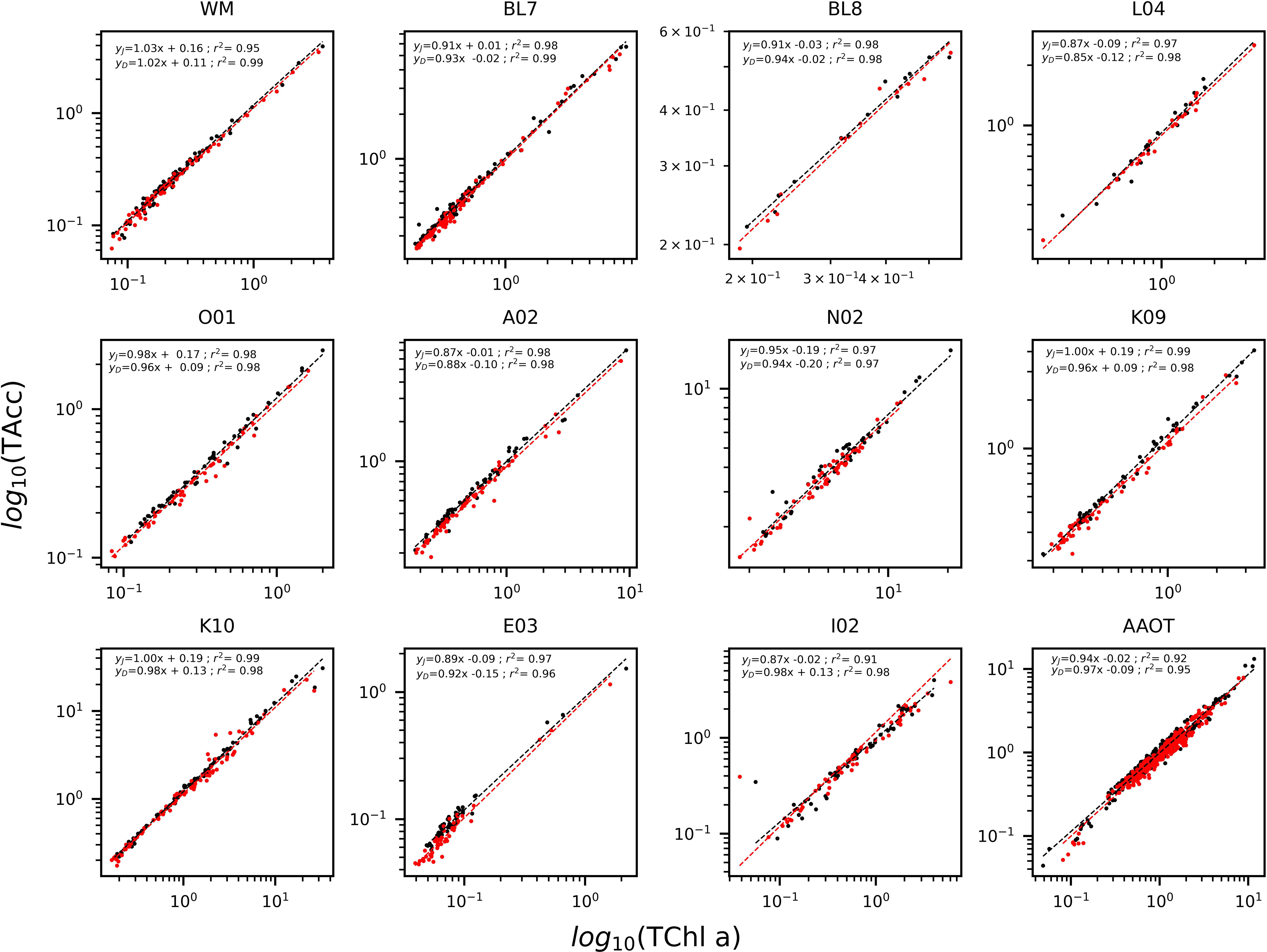
Figure 2 Log-linear regression of accessory pigments (TAcc) versus TChl a for the Oceanographic Campaigns and the AAOT for J (black) and D (red). Data are presented in log10 scale.
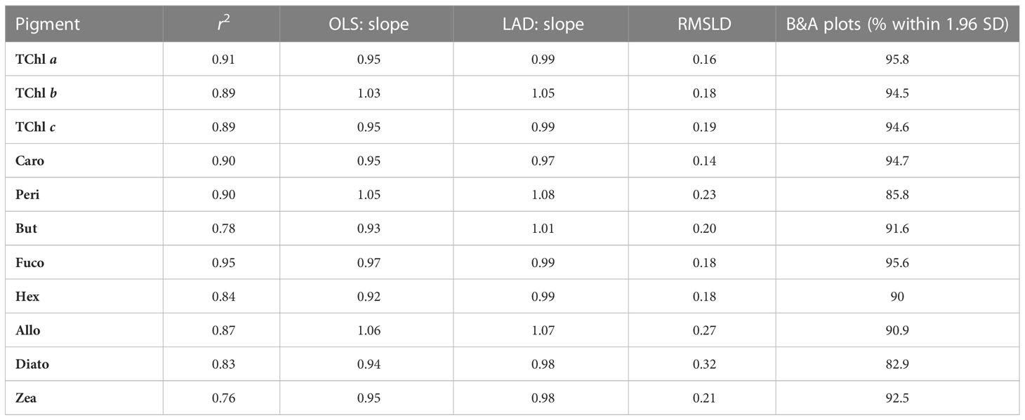
Table 6 Summary of the results of linear regression analysis applied to log-transformed data (OLS and LAD), root mean squared logarithmic difference (RMSLD), and of the Bland–Altman (B&A) plots.
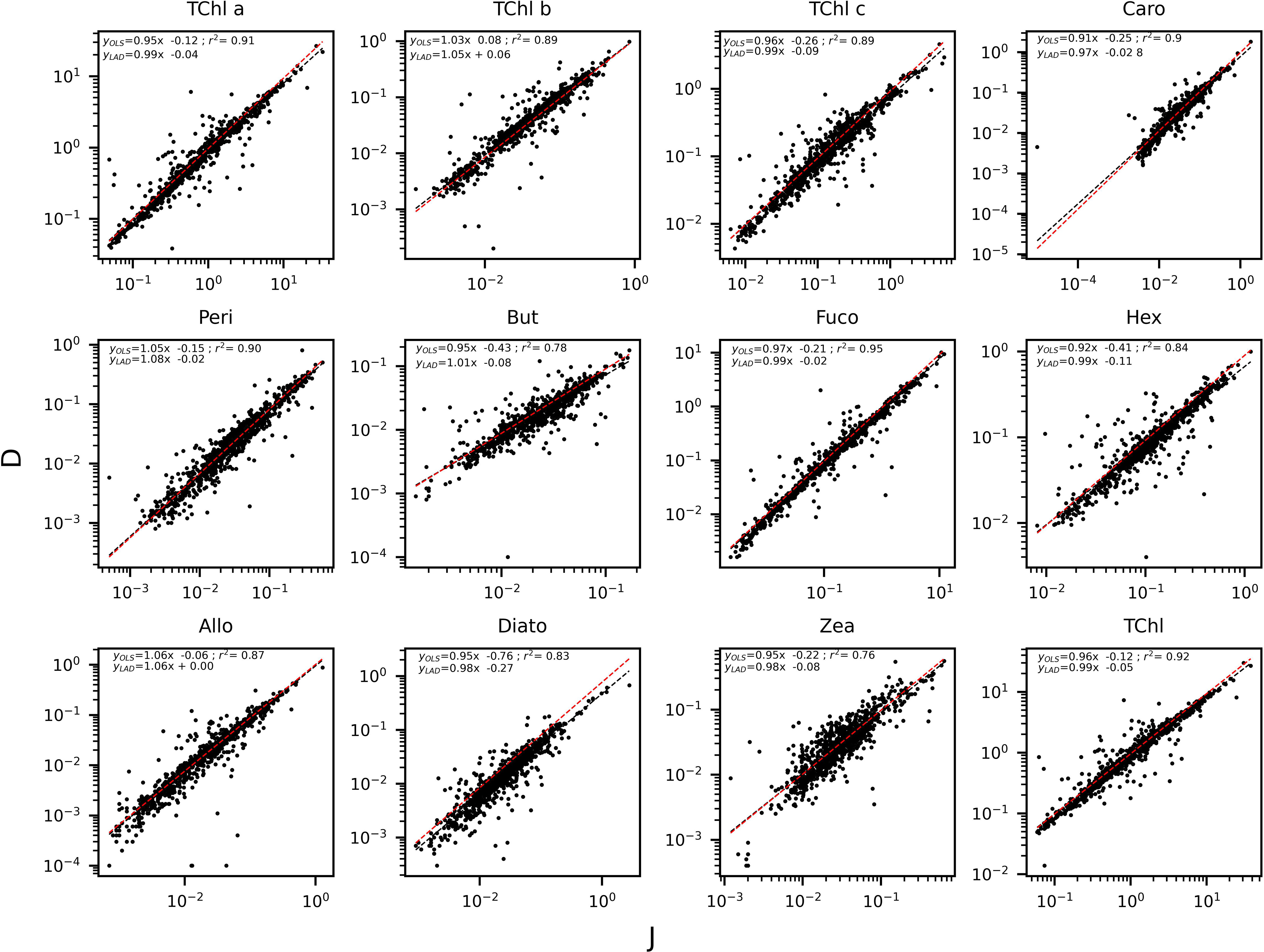
Figure 3 Regression applied to the log transformed value of the PPig: curve and equation for OLS (in black) and LAD (in red).
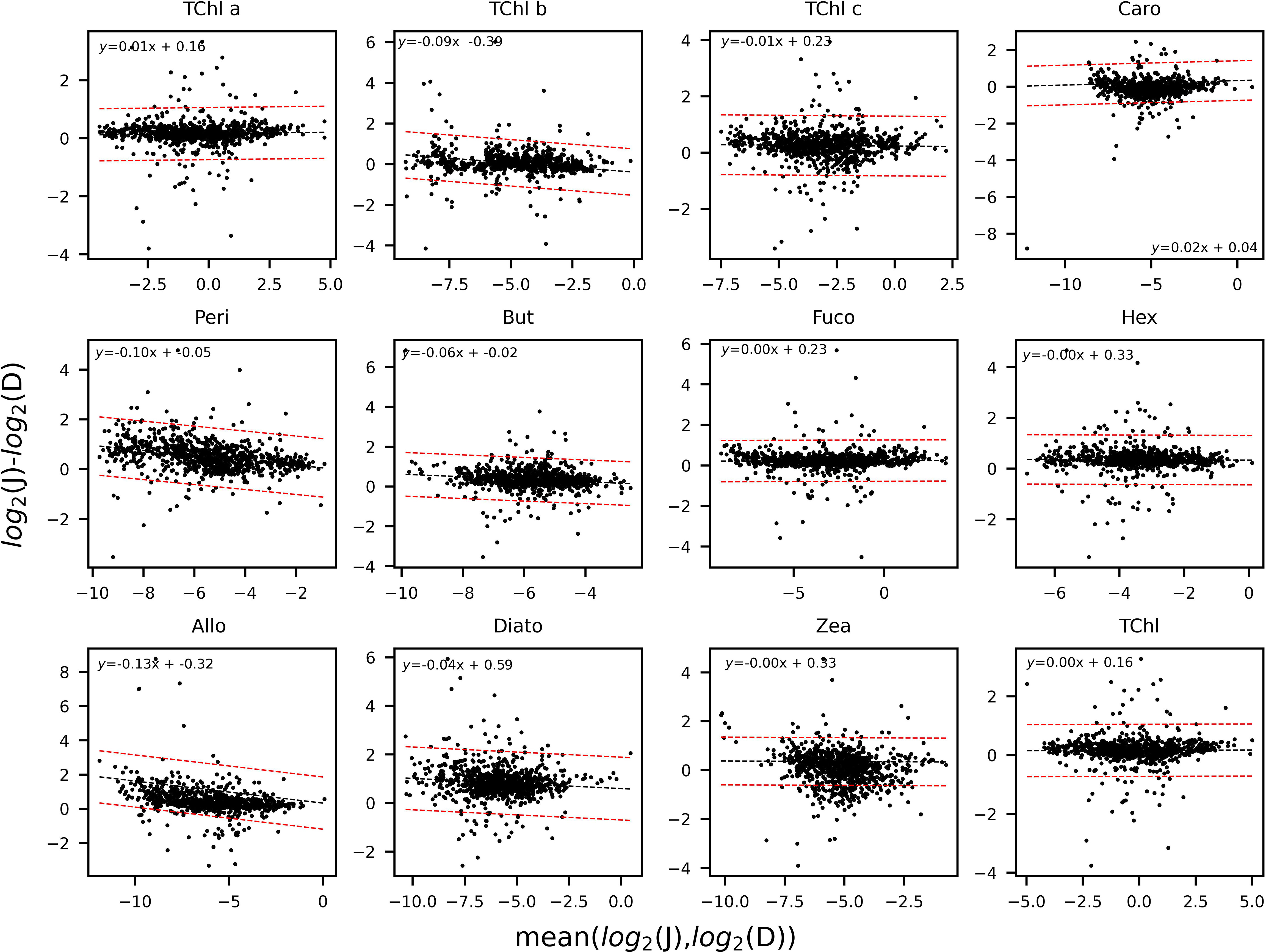
Figure 4 Bland and Altman plots for the PPig: TChl a, TChl b, TChl c, Caro, Peri, But, Fuco, Hex, Allo, Diato, Zea, and the TChl. The limit of agreement, in red, encompasses the data points within 1.96 standard deviations. The trend-line between the two laboratories is in black.
Coherently with the B&A plots, %PD tends to be higher for lower values of the pigment concentration: the %PD highest values (> 50%) are seen for all pigments at concentrations lower than 0.5 mg/m3 (Figure 5). With measurement stations located mostly in clear or only moderately turbid waters (Figure 1), most of the samples analyzed in support to this comparison had concentrations in the range of 0.05–0.5 mg/m3 for PPig and lower than 0.05 mg/m3 for the secondary pigments (Figure 5; Table 7). Lower correlations between laboratories occurred when pigments were quantified close to the instrumental LOD. This behavior has already been observed in previous intercomparisons and confirmed that the false-positive/negative quantifications performed near LOD thresholds may cause an increase in the bias (Hooker et al., 2005; Canuti et al., 2016). Considering the whole data set, J overestimates TChl a by 10.6% and PPig by 16.9% (Table 8), confirming the presence of a systematic bias as suggested by the B&A plot analysis. The analytical method had an impact on the distribution of differences among pigments. In this regard, we could observe that for all the campaigns, %PD were lower (−5.8%) for Caro and close to 0 for Zea and TChl b (−0.3% and 0.9%, respectively), despite the fact that the concentration of Zea was lower than 1 mg/m3 for all the samples. In the absence of specific tests on extraction on replicates of natural samples and of the analysis of common standards, it is not possible to attribute observed differences to the extraction procedure, to the chromatographic separation, or to a combination of the two.
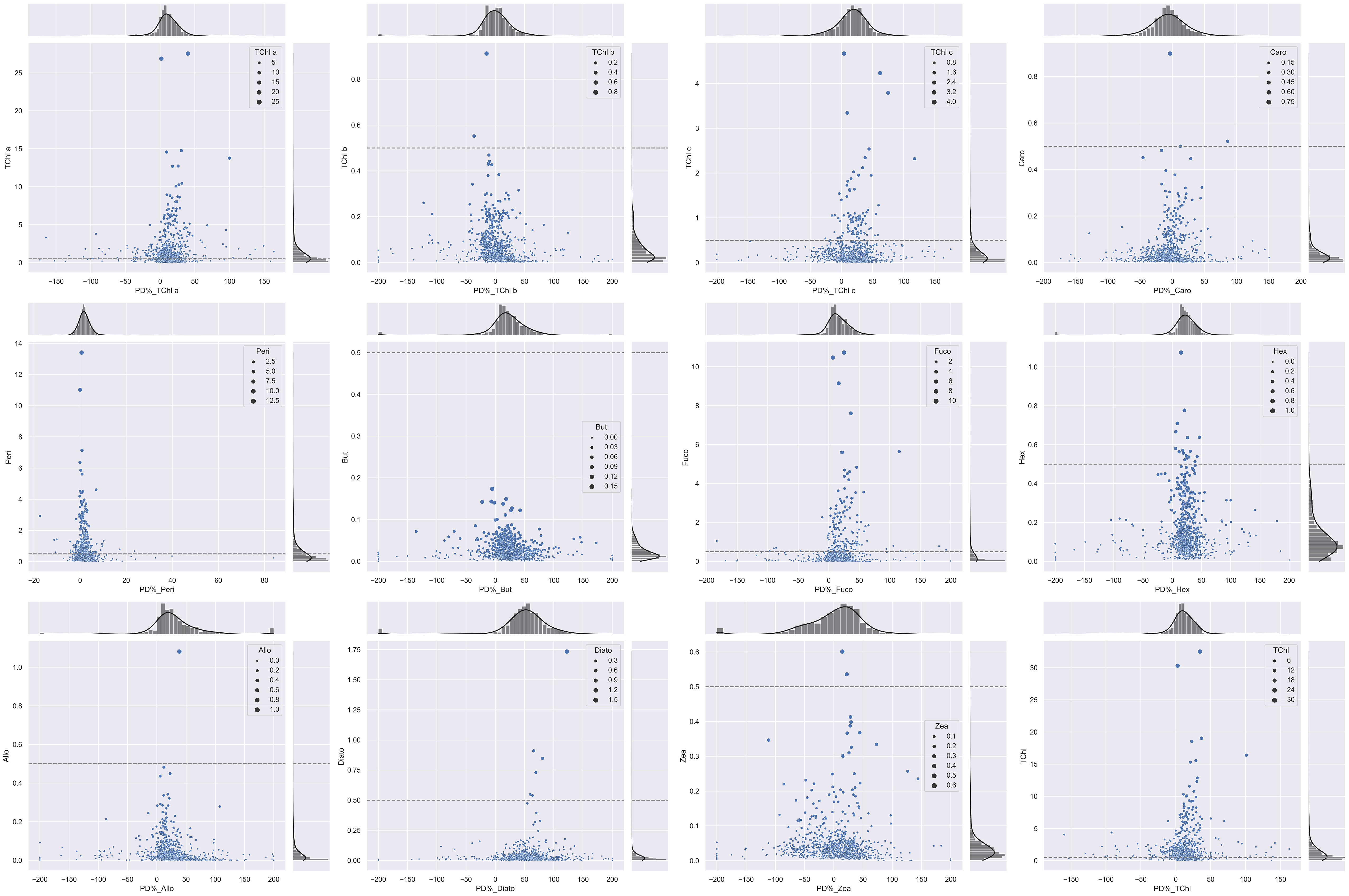
Figure 5 Scatter plot displaying invariant histograms of the marginal distribution for PD% and pigment concentrations (mg/m3). The horizontal and vertical axes represent TChl a, TChl b, TChl c, Caro, Peri, But, Fuco, Hex, Allo, Diato, Zea, and TChl. The dashed lines indicate the 0.5-mg/m3 threshold for each primary pigment, and the legend corresponds to each pigment concentration.
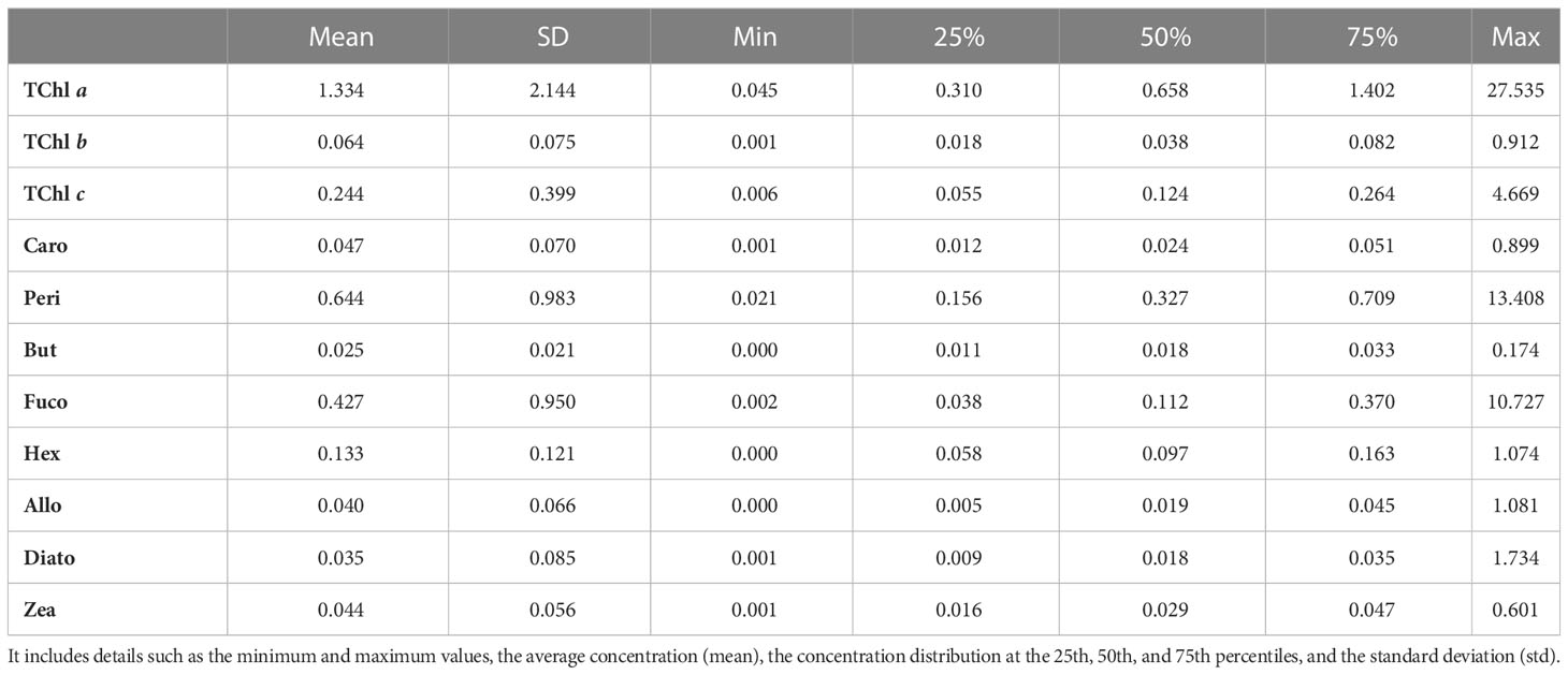
Table 7 Summary of the distribution of PPig concentration throughout the entire dataset (in mg/m3).
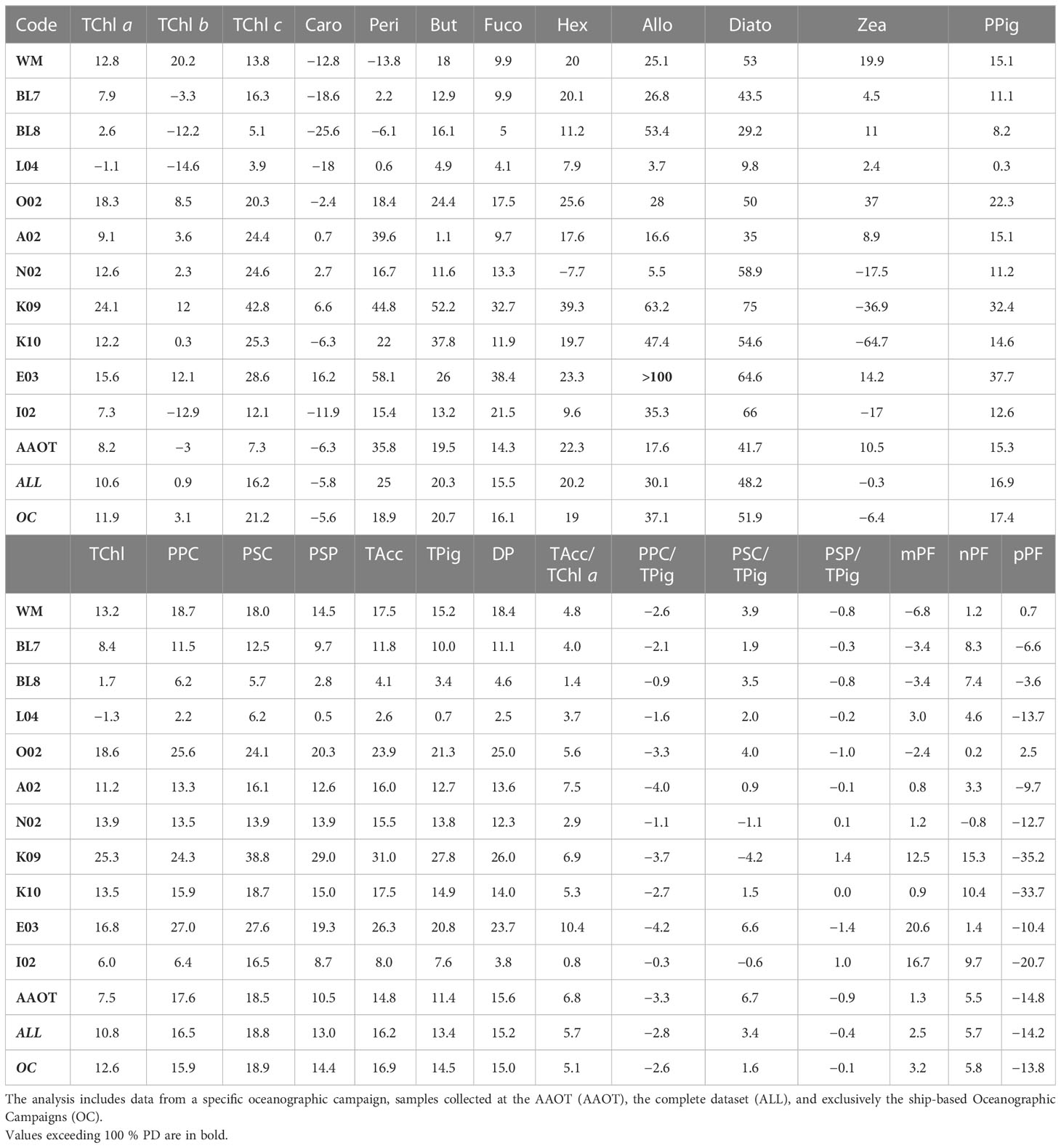
Table 8 Overview of the unbiased percentage difference (%PD) across various parameters (PPig, PSum, PRatios, and PIndices) comparing two laboratories.
The closest results between the laboratories were observed for the samples collected on AAOT: for TChl a, the average %PD is 8.2% versus 11.9% for the ship-based oceanographic campaigns and 15.3% versus 17.4% for what concerns the PPig. This could be explained by the large number of campaigns and major confidence in the filtration procedure (i.e., the volume of water to use for preconditioning the filter) and by the fact that, proportionally, the most oligotrophic conditions (associated with high %PD) were mostly found during oceanographic campaigns. The comparison of the surface data (one third of the total AAOT samples) with samples collected at 8 and 14 m depth exhibits comparable %PD for TChl a. Differences in results between AAOT and oceanographic campaigns also suggest that the inhomogeneity of preconditioned samples may affect the assumed equivalence of duplicates and consequently the agreement between independent analyses, regardless of the pigment concentration.
The %PD was further considered in relation to the sampling campaign (all results detailed in Table 8) to evaluate if the water type and a change in the operator, generating an inhomogeneity in the duplicate samples, may also impact the difference distribution. It can be noticed that when the TChl a average concentration is close to 1 mg/m3 (campaigns L04, BL7, I02 and AAOT), the %PD values (in modulus) are lower (from −1% to 8%), independently from the marine basin considered. This suggests that the methods are optimized for analysis of samples with a TChl a pigment content around 1 mg/m3. Other considerations, considering the differences between campaigns, indicate that an increase in %PD for low concentrations is by no means a general rule. The E03 (Eastern Mediterranean Sea) and K09 (Black Sea) campaigns had a comparable number of samples (49 and 53 respectively), were performed within a year, and finally, the time delay between collection and analysis was comparable. E03 TChl a concentration was on average noticeably lower than during K09 (0.098 and 0.678 mg/m3, respectively), but the associated PD% is 15.6%, while it is 24.1% for K09 (Table 8). Similar differences could be appreciated considering the %APD, where the TChl a associated with E03 is 16.9% while itis 26.3% during K09 (Table 9). On the other hand, the BL8 campaign (Black Sea, TChl a of 0.413 mg/m3 on average) shows lower differences (2.6% for TChl a and 8.2% for PPig) than K09. We could conclude that the marine basin and the water type are not influencing the performance of the two laboratories.
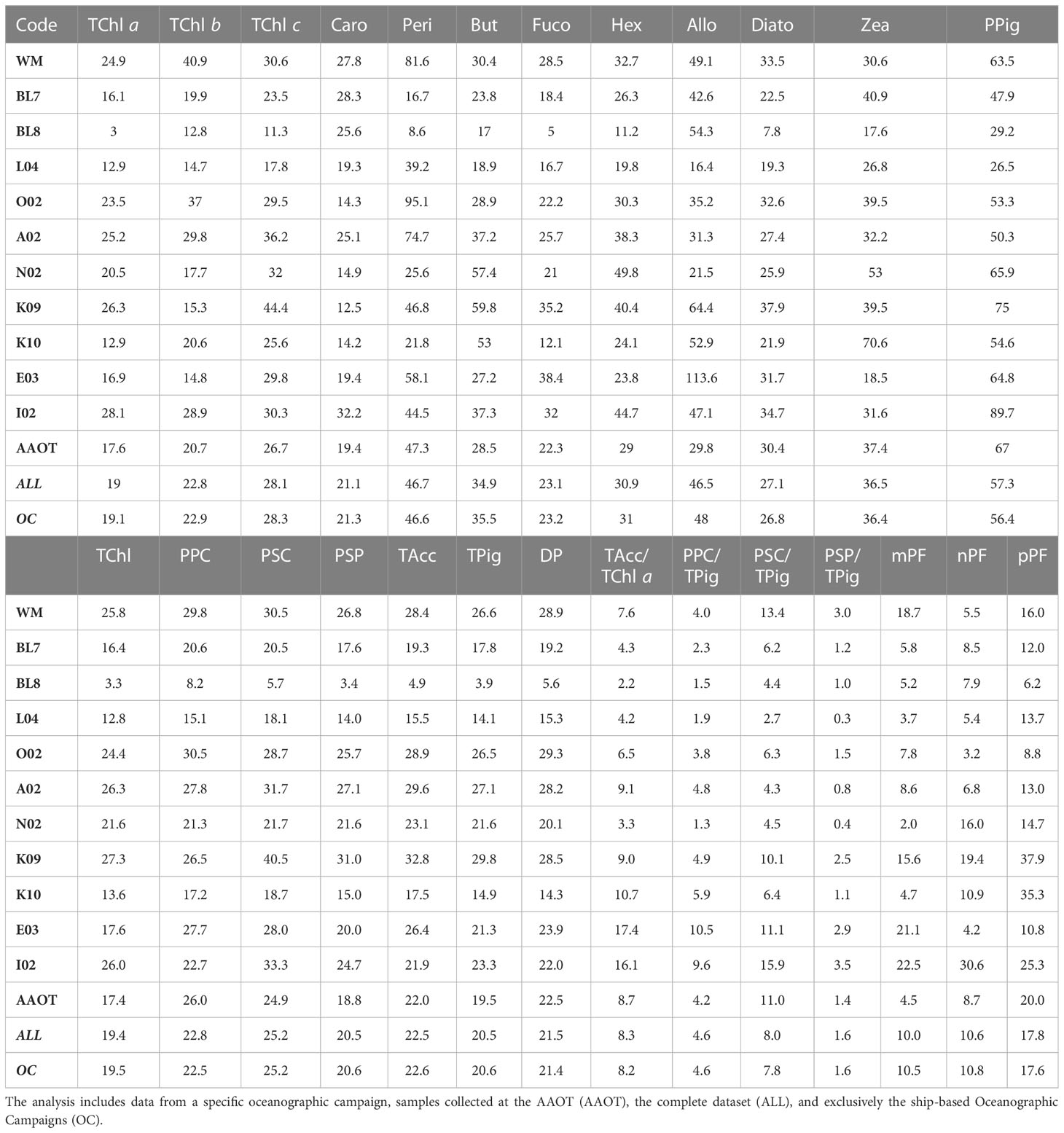
Table 9 Overview of the absolute percentage difference (%APD) across various parameters (PPig, PSum, PRatios, and PIndices) comparing two laboratories.
Sample storage was considered as well. In a few cases, the samples were analyzed at different times by the two laboratories. J analyzed the WM campaign’s samples 5 years after their collection. It was expected that for these samples the MVChl a could be partially degraded in DVChl a and Chlide a. Jeffrey et al. (1997) recovered 98% and 83% of the original TChl a concentration in microalgae after storage at −196°C for 60 and 328 days, respectively. WM was compared with E03 and I02 campaigns, where E03 and I02 samples were analyzed within a year from collection and no degradation of MVChl a is expected (Jeffrey et al., 1997). The TChl a results for the three campaigns are comparable to what is observed over all the stations: J overestimated D by 12.8% for WM, 15.6% and 7.3%, respectively, for E03 and I02 (Table 8). The MVChl a is on average 9.9% higher for J with respect to D. We should thus expect a lower overestimation of MVChl a for WM with respect to E03 and I02 due to an increasing contribution of Chlide a and DVChl a to TChl a. In the WM campaign, MVChl a quantified by J was 13.8% higher than D’s value, while this overestimation is 17.8% in the case of E03, and is not observed for I02, with J and D values of MVChl a very close (J< D by 0.9%). In the good analysis practice, 1 year is considered the maximum interval between sample collection and analysis (Jeffrey et al., 1997) The case described here indicates that time longer than 1 year between collection and analyses (5 years for WM) did not appear to affect the final quantification of TChl a.
It was expected that for higher-level variables (i.e., pigment sum, see Table 2) the differences between J and D should decrease as the concentration increases (Tables 8, 9). The TChl and DP generally follow the expected trend (differences between laboratories over all samples of 10.8% and 15.2%, respectively). TPig and other sums show differences around 15%, similar to or lower than those encountered for the single PPig. As for the pigment indexes PIndex used to evaluate the proportion for micro- (mPF), nano- (nPF), and picoplankton (pPF), the difference is low for the mPF and nPF fractions (2.5% and 5.7%, respectively, and of 10.0% and 10.6% APD), and higher for pPF (−14.2% PD and 17.8%APD). Looking at results across campaigns, it can be observed that pPF was high (unbiased %PD of −35.2% and −33.7% and %APD of 37.9% and 35.3%, respectively) for the K09 and K10 campaigns (Black Sea, late summer) but not so for BL7 and BL8 (Black Sea, early summer), where the values are −6.6% and −3.6% for pPF, respectively (12.0% and 6.2%, if we considered the %APD), thus suggesting that the basin itself is not a source of differences. The %PD values of mPF and nPF are usually found below 10% (in modulus).
The average %PD can be interpreted in terms of accuracy for the concentration of the various pigments. Accuracy estimates can be fed into error propagation techniques applied to algorithms dedicated to the calculation of PFT’s abundance or PSCs (e.g., Mouw et al., 2017). Additional information required for error propagation is the possible error correlation existing among pairs of pigments. This point has been explored here by using the 611 stations of the oceanographic campaigns and correlating the difference J–D for pairs of diagnostic pigments (Table 10). In general, the correlation (i.e., Pearson correlation coefficient) between differences is fairly low, but there are cases where the correlation is close to or exceeds 0.5. The highest being between TChl a and Fuco (> 0.9), other remarkable correlations were found between TChl a and Caro and TChl c (> 0. 7), and similarly between Fuco and TCl c and Caro (> 0.7).
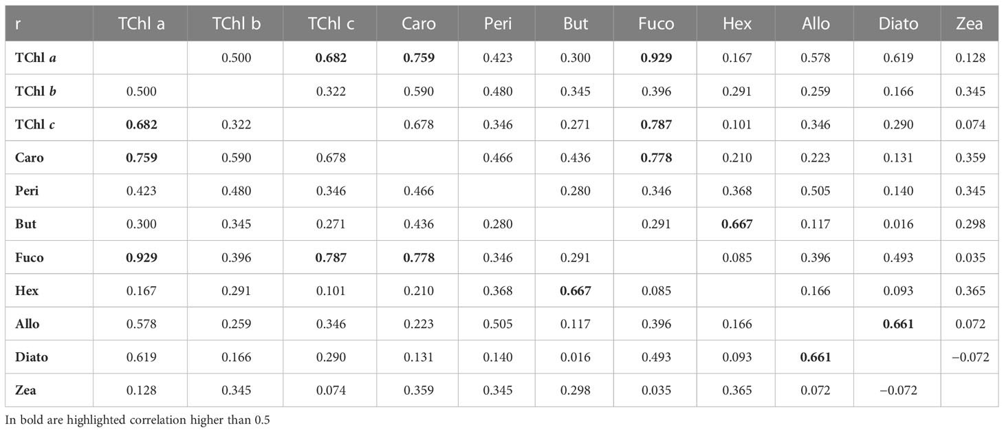
Table 10 Pearson correlation coefficient, r, between the differences (J minus D) for the diagnostic pigments.
To quantify the impact that uncertainties on pigment concentrations might have on PFTs and PSCs, the pigment distributions from the two laboratories were independently used as input to the model of Hirata et al. (2011) (summarized in Table 3), with results elaborated with the Data-Interpolating Variational Analysis (DIVA) software tool of the Ocean Data View software (https://odv.awi.de) to visualize the observations spatially interpolated (Figure 6). These maps should not be interpreted as actual PFT or PSC distributions, as oceanographic campaigns in a given basin took place in different periods, but they offer an efficient overview of the agreement between the distributions obtained from the two data sets. In general, the J and D distributions appear fairly coherent, with some exceptions. PSCs show a good agreement, confirming the results obtained for the pigment index (Tables 8, 9), which is not surprising as the formula are comparable. The picoplankton fraction observed in the Black Sea shows some differences between J and D in line with those observed for pPF in this specific basin (particularly for K09 and K10). For PFTs, the largest differences are seen for diatoms (higher values for J) and, to a much lesser extent, for dinoflagellates.
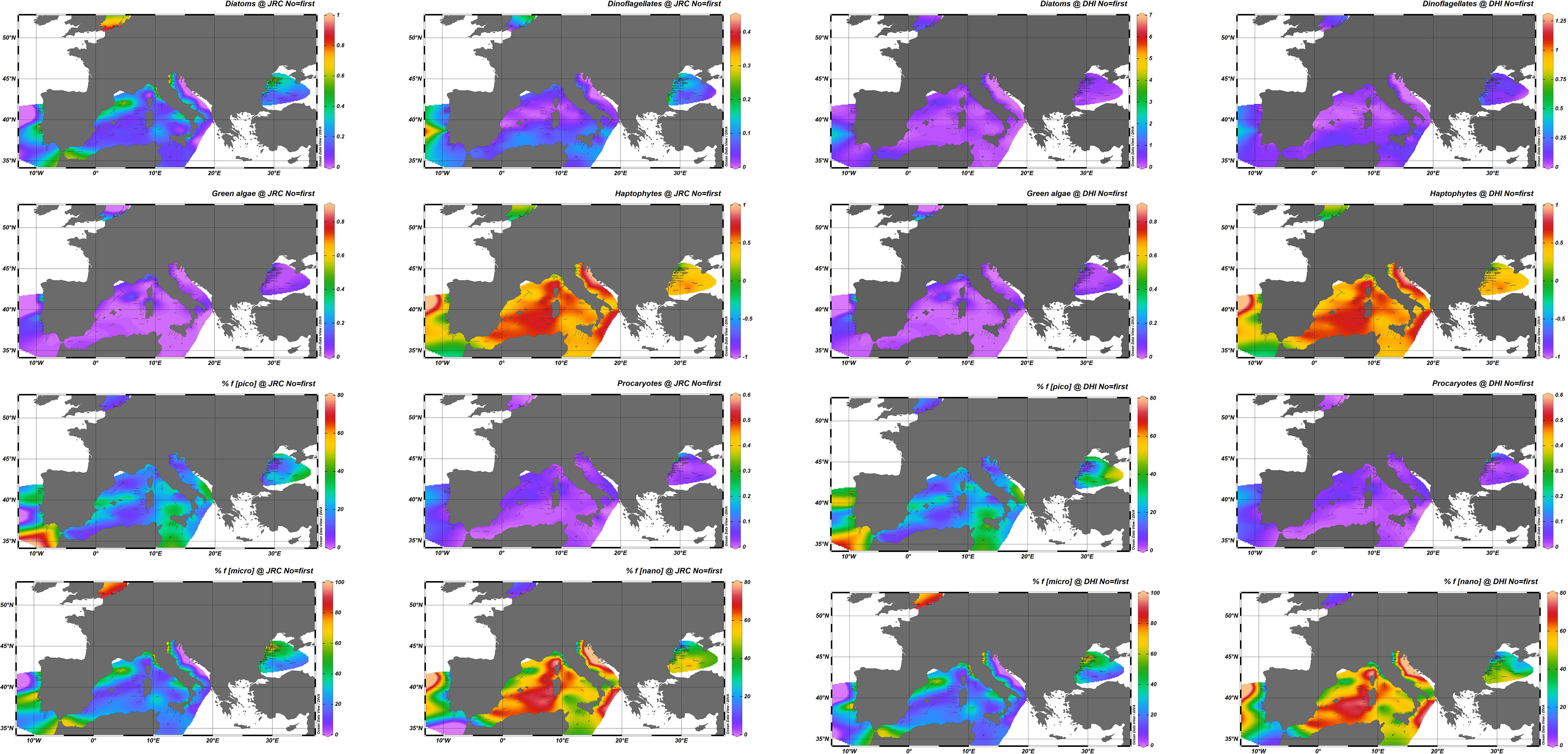
Figure 6 Synoptic distribution of surface PFTs (diatoms, dinoflagellates, green algae, haptophytes, procaryotes) expressed as fraction 0–1 of the TChl a and PSCs (pico-, nano-, microplankton expressed as) % fraction of the TChl a for J and D datasets. The DIVA software tool (Data-Interpolating Variational Analysis) of the Ocean Data View (ODV) software is used for spatial interpolation.
4 Discussion and conclusions
The present exercise relied on a unique data set of 957 measurement stations covering several European basins, for which samples could be analyzed for pigment concentration by two quality-certified laboratories. An average difference of 10.6% was observed for TChl a for concentrations across a wide range of values (0.083 to 27.35 mg/m3). If interpreted in terms of accuracy, this result fully satisfies the requirement of a 15% accuracy threshold associated with TChl a, measurement recommended for the validation of satellite data products. The average differences for PPig is 16.9%, with systematic differences (biases) observed for the J values of PPig with respect to those from D for chlorophylls and several xanthophylls. However, for some pigments (i.e., Zea and Caro), the differences are close to 0 or very low, regardless of the pigment concentration or the basin considered. This indicates that the extraction methods employed by the laboratories may diversely influence the quantification results in relation to the pigment’s chemical structure. Overall, differences between J and D were lowest for natural samples containing approximately 1 mg/m3 of TChl a, suggesting that both methods are optimized for a target analysis around this concentration.
Other aspects observed concern the time of preservation and the homogeneity of the samples. In terms of preservation, for the Western Mediterranean Sea oceanographic campaign, the long time between collection and analyses (5 years) does not appear to affect the final quantification of TChl a. On the other hand, the analysis of the data set by single campaign suggested that in several cases, the difference between laboratories could result from the in-homogeneity of duplicate samples, regardless of the pigments concentration or the basin characteristics, but in the absence of series of replicates, it was not possible to support this correlation statistically. In the intercomparison exercises, where the participants are usually four laboratories or more, the distribution of triplicates of each natural sample together with the analysis of standards provided to all the participants, allows to clearly address if the statistical differences among participants are due to the methods or to the samples inhomogeneity.
As for the higher-level variables, the differences between laboratories are, of course, in line with the results given for the individual pigments. The average difference for TChl a and DP is 10.8% and 15.2%, respectively. Pigment indexes, which are simple indicators for PSCs, showed a good agreement, with larger differences for the picoplankton fraction pPF (average of 14%) that can be explained by larger differences observed for Zea. This result for pPF can also be traced to the impact of two Black Sea campaigns (K09 and K10) that usually show higher differences for all quantities. In view of developing error propagation models for PFT or PSC algorithms, the analysis correlating differences between the two laboratories indicates a modest degree of error correlation, but exceptions suggest the need for further investigation. It is nevertheless stressed that this result is valid for in situ pigment data and would not necessarily apply to pigment concentration obtained by dedicated algorithms.
In general, it was observed that, regardless of the pigment concentration, the inhomogeneity in the water sample preparation may affect the assumed equivalence of duplicates and consequently the agreement between independent analyses. In conclusion, the comparison with an accredited laboratory is a good option for developing a new method or continuously assessing an existing one. To take one step further and properly address the differences between laboratories, the comparison should include certified standards analyzed at regular time intervals and, in the case of natural sample collection, a series of replicates (minimum three to be analyzed by each laboratory) to build a proper statistic on the natural samples collected. As illustrated by this study and previous intercomparison exercises, defining uncertainty values associated with single in situ pigment measurement is no easy task, but it is required to promote pigment data as fiducial reference measurements. It would also be a good practice before ingesting pigment data into global data bases of pigment data.
Data availability statement
The raw data supporting the conclusions of this article will be made available by the authors, without undue reservation.
Author contributions
EC has made contributions to this paper in the areas of conception, study design, analytic performance, and calculation.
Funding
The study has been supported by the European Commission Directorate-General for Defense, Industry and Space (DG DEFIS) and the Copernicus Programme.
Acknowledgments
The author would like to acknowledge all colleagues who alternated in the collection of the samples replicated in the different BiOMaP cruises and AAOT campaigns. Support provided by the European Commission Directorate-General for Defense, Industry and Space (DG DEFIS) and the Copernicus Programme is gratefully acknowledged.
Conflict of interest
The author declares that the research was conducted in the absence of any commercial or financial relationships that could be construed as a potential conflict of interest.
Publisher’s note
All claims expressed in this article are solely those of the authors and do not necessarily represent those of their affiliated organizations, or those of the publisher, the editors and the reviewers. Any product that may be evaluated in this article, or claim that may be made by its manufacturer, is not guaranteed or endorsed by the publisher.
References
Aiken J., Pradhan Y., Barlow R., Lavender S., Poulton A., Holligan P., et al. (2009). Phytoplankton pigments and functional types in the Atlantic ocean: a decadal assessment 1995-2005. Deep Sea Res. Part II: Topical Stud. Oceanography 56 (15), 899–917. doi: 10.1016/j.dsr2.2008.09.017
Bland J. M., Altman D. G. (1986). Statistical methods for assessing agreement between two methods of clinical measurement, the lancet 327, 8476, 307–310. doi: 10.1016/S0140-6736(86)90837-8
Bland J. M., Altman D. G. (1995). Comparing methods of measurement: why plotting difference against standard method is misleading. Lancet. 346, 1085–1087. doi: 10.1016/S0140-6736(95)91748-9
Bland J. M., Altman D. G. (1999). Measuring agreement in method comparison studies. Stat. Methods Med. Res. 8, 135–160. doi: 10.1177/096228029900800204
Bracher A., Bouman H. A., Brewin R. J. W., Bricaud A., Brotas V., Ciotti A. M., et al. (2017). Obtaining phytoplankton diversity from ocean color: a scientific roadmap for future development. Front. Mar. Sci. 4. doi: 10.3389/fmars.2017.00055
Brewin R. J. W., Sathyendranath S., Hirata T., Lavender S. J., Barciela R. M., Hardman-Mountford N. J. (2010). A three-component model of phytoplankton size class for the Atlantic ocean ecological modelling. Ecol. Model. 221, 11, 1472–1483. doi: 10.1016/j.ecolmodel.2010.02.014
Canuti E., Artuso F., Bracher A., Brotas V., Devred E., Dimier C., et al. (2022). The fifth HPLC intercomparison on phytoplankton pigments (HIP-5) technical report, EUR 31334 EN (Luxembourg: Publications Office of the European Union). doi: 10.2760/563102
Canuti E., Ras J., Grung M., Röttgers R., Costa Goela P., Artuso F., et al. (2016). HPLC/DAD intercomparison on phytoplankton pigments (HIP-1, HIP-2, HIP-3 and HIP-4), EUR 28382 EN (Luxembourg: Publications Office of the European Union).
Claustre H., Hooker S. B., Van Heukelem L., Berthon J.-F., Barlow R., Ras J., et al. (2004). An intercomparison of HPLC phytoplankton methods using in situ samples: application to remote sensing and database activities. Mar. Chem. 85, 41–61. doi: 10.1016/j.marchem.2003.09.002
EURACHEM/CITAC Guideline (2000). Quantify uncertainties in analytical measurements, 2nd edition. Available at: https://eurachem.org/index.php/publications/pubarch/81-gdquam20002.
GCOS (2011). “Systematic observation requirements for satellite-based products for climate,” in GCOS-154, supplemental details to the satellite-based component of the “Implementation plan for the global observing system for climate in support of the UNFCC". Geneva: UNFCC.
Hirata T., Hardman-Mountford N. J., Brewin R. J. W., Aiken J., Barlow R., Suzuki K., et al. (2011). Synoptic relationships between surface chlorophyll- a and diagnostic pigments specific to phytoplankton functional types. Biogeosciences 8, 311–327. doi: 10.5194/bg-8-311-2011
Hooker S. B., Clementson L., Thomas C. S., Schluter L., Allerup M., Ras J., et al. (2012). The fifth SeaWiFS HPLC analysis round-robin experiment (SeaHARRE-5) NASA tech (Greenbelt, Maryland: NASA Goddard Space Flight Center), 95.
Hooker S. B., Thomas C. S., Van Heukelem L., Schluter L., Ras J., Claustre H., et al. (2010). The forth SeaWiFS HPLC analysis round-robin experiment (SeaHARRE-4) NASA tech (Greenbelt, Maryland: NASA Goddard Space Flight Center), 74.
Hooker S. B., Van Heukelem L., Thomas C. S., Claustre H., Ras J., Barlow R., et al. (2005). The second SeaWIFS HPLC analysis round-robin experiemnt /SeaHARRE-2).
Hooker S. B., Van Heukelem L., Thomas C. S., Claustre H., Ras J., Schluter L., et al. (2009). The third SeaWiFS HPLC analysis round-robin experiment (SeaHARRE-3) NASA tech (Greenbelt, Maryland: NASA Goddard Space Flight Center), 106.
IOCCG (2014). Phytoplankton functional types from space. in Reports of the International Ocean-Colour Coordinating Group, No. 15. Ed. Sathyendranath S. (Dartmouth, Canada: IOCCG), 156.
Jeffrey S. W., Mantoura R. F. C., Wright S. W. (1997). “Monographs on oceanographic methodology,” in Phytoplankton pigments in oceanography (Paris: UNESCO).
JGOFS Protocols for the Joint Global Ocean Flux Study Core Measurements (1994). “Intergovernmental oceanographic commission, scientific Committee on oceanic research,” in Manual and guides, vol. 29. (Paris: UNESCO), 91–96.
Latasa M., Bidigare R. R., Ondrusek M. E., Kennicutt. M. C. (1996). HPLC analysis of algal pigments: a comparison exercise among laboratories and recommendations for improved analytical performance. Mar. Chem. 51, 315–324. doi: 10.1016/0304-4203(95)00056-9
Mackey M., Mackey D., Higgins H. W., Wright S. W. (1996). CHEMTAX - a program for estimating class abundances from chemical markers: application to HPLC measurements of phytoplankton. Mar. Ecol. Prog. Ser. 144, 265–283. doi: 10.3354/meps144265
Matsumoto T., Shinozaki F., Chikuni T., Yabuki A., Takishita K., Kawachi M., et al. (2011). Green-colored plastids in the dinoflagellate genus Lepidodinium are of core chlorophyte origin. Protist 162 (2), 268–276. doi: 10.1016/j.protis.2010.07.001
Mouw C. B., Hardman-Mountford N. J., Alvain S., Bracher A., Brewin R. J. W., Bricaud A., et al. (2017). A consumer’s guide to satellite remote sensing of multiple phytoplankton groups in the global ocean. Front. Mar. Sci. 4. doi: 10.3389/fmars.2017.00041
Naik R. K., Anil A. C., Narale D. D., Chitari R. R., Kulkarni V. V. (2011). Primary description of surface water phytoplankton pigment patterns in the bay of Bengal. J. Sea Res. 65 (4), 435–441. doi: 10.1016/j.seares.2011.03.007
Roy S., Llewellyn C., Egeland E., Johnsen G. (2011). “Phytoplankton pigments: characterization, chemotaxonomy and applications in oceanography,” in Cambridge Environmental chemistry series (Cambridge: Cambridge University Press), 314–342.
Schlüter L., Behl S., Striebel M., Stibor H. (2016). Comparing microscopic counts and pigment analyses in 46 phytoplankton communities from lakes of different trophic state. Freshw. Biol. 61, 1627–1639. doi: 10.1111/fwb.12803
Trees C. C., Clark D. K., Bidigare R. R., Ondrusek M. E., Mueller J. L. (2000). Accessory pigments versus chlorophyll a concentrations within the euphotic zone: a ubiquitous relationship. Limnol. Oceanogr. 5, 1130–1143. doi: 10.4319/lo.2000.45.5.1130
Uitz J., Claustre H., Morel A., Hooker S. B. (2006). Vertical distribution of phytoplankton communities in open ocean: an assessment based on surface chlorophyll. J. Geophys. Res. 111, C08005. doi: 10.1029/2005JC003207
Van Heukelem L., Thomas C. S. (2001). Computer-assisted high performance liquid chromatography method development with applications to the isolation and analysis of phytoplankton pigments. J. Chromatogr. A 910 (1), 31–49. doi: 10.1016/S0378-4347(00)00603-4
Vidussi F., Claustre H., Manca B., Lucchetta A., Marty J. C. (2001). Phytoplankton pigment distribution in relation to upper thermocline circulation in the eastern Mediterranean Sea during winter. J. Geophys. Res. 136 (C9), 19,939–19,956. doi: 10.1029/1999JC000308
Wasmund N., Topp I., Schories D. (2006). Optimising the storage and extraction of chlorophyll samples. Oceanologia 48 (1), 177–186.
Wright S. W., Jeffrey S. W. (2005). “Pigment markers for phytoplankton production,” in Marine organic matter: biomarkers, isotopes and DNA. the handbook of environmental chemistry, vol. 2N . Ed. Volkman J. K. (Berlin, Heidelberg: Springer).
Wright S. W., Jeffrey S. W., Mantoura R. F. C., Llewellyn C. A., Bjornland T., Repeta D., et al. (1991). Improved HPLC method for the analysis of chlorophylls and carotenoids from marine phytoplankton. Mar. Ecol. Prog. Ser. 77, 183–196. doi: 10.3354/meps077183
Xi H., Losa S. N., Mangin A., Garnesson P., Bretagnon M., Demaria J. (2021). Global chlorophyll a concentrations of phytoplankton functional types with detailed uncertainty assessment using multi-sensor ocean color and sea surface temperature satellite products. J. Geophys. Res.: Oceans 126, e2020JC017127. doi: 10.1029/2020JC017127
Xi H., Losa S. N., Mangin A., Soppa M. A., Garnesson P., Demaria J., et al. (2020). Global retrieval of phytoplankton functional types based on empirical orthogonal functions using CMEMS GlobColour merged products and further extension to OLCI data. Remote Sens. Environ. 240, 111740. doi: 10.1016/j.rse.2020.111704
Zapata M., Rodriguez F., Garrido J. L. (2000). Separation of chlorophylls and carotenoids from marine phytoplankton: a new HPLC method using reverse phase C8 column and pyridine-containing mobile phase. Mar. Ecol. Prog. Ser. 195, 29–45. doi: 10.3354/meps195029
Keywords: chlorophyll a, phytoplankton pigments, HPLC, inter-laboratory comparison, uncertanties
Citation: Canuti E (2023) Phytoplankton pigment in situ measurements uncertainty evaluation: an HPLC interlaboratory comparison with a European-scale dataset. Front. Mar. Sci. 10:1197311. doi: 10.3389/fmars.2023.1197311
Received: 30 March 2023; Accepted: 24 May 2023;
Published: 19 June 2023.
Edited by:
Gemma Kulk, Plymouth Marine Laboratory, United KingdomReviewed by:
Ravidas Krishna Naik, National Centre for Polar and Ocean Research (NCPOR), IndiaJoanna Stoń-Egiert, Polish Academy of Sciences, Poland
Copyright © 2023 Canuti. This is an open-access article distributed under the terms of the Creative Commons Attribution License (CC BY). The use, distribution or reproduction in other forums is permitted, provided the original author(s) and the copyright owner(s) are credited and that the original publication in this journal is cited, in accordance with accepted academic practice. No use, distribution or reproduction is permitted which does not comply with these terms.
*Correspondence: Elisabetta Canuti, ZWxpc2FiZXR0YS5jYW51dGlAZWMuZXVyb3BhLmV1