Multi factors-PredRNN based significant wave height prediction in the Bohai, Yellow, and East China Seas

Introduction: Currently, deep-learning-based prediction of Significant Wave Height (SWH) is mostly performed for a single location in the ocean or simply relies on a single factor (SF). Such approaches have the disadvantage of lacking spatial correlations or dynamic complexity, leading to an inevitable growth of the prediction error with time.

Methods: Here, attempting a solution, we develop a Multi-Factor (MF) data-driven 2D SWH prediction model for the Bohai, Yellow, and East China Seas (BYECS). Our model is developed based on a multi-channel PredRNN algorithm that is an improved deep-learning calculation of the ConvLSTM.

Results: In our model, the MF of historical SWH, 10 m surface winds, ocean surface currents, bathymetries, and open boundaries are used to predict 2D SWH in the next 1-72h. Our modeled SWHs show the correlation coefficients as 0.98, 0.90, and 0.87 for the next 6h, 24h, and 72h, respectively.

Discussion: According to the ablation experiments, winds are the dominant factor in the MF model and the memory-decoupling module is the key improvement of the PredRNN compared to the ConvLSTM. Furthermore, when the historical SWH is excluded from the input, the correlation coefficients remain around 0.95 in the 1-72h prediction due to the elimination of the error accumulation. It was worse than the MF-PredRNN with the historical SWH before 10h but better than it after 10h. Overall, for the prediction of SWH in the BYECS, our MF-PredRNN-based 2D SWH prediction model significantly improves the accuracy and extends the effective prediction time length.

1 Introduction

Ocean waves (hereinafter referred to as waves) are the most common phenomenon in the ocean. Waves of extreme heights have been regarded as marine disasters that threaten maritime operations and navigation (Mahjoobi and Mosabbeb, 2009), and thus wave forecasting has been an essential and indispensable routine in maritime institutions worldwide (Gao et al., 2021).

As a most important parameter, the Significant Wave Height (SWH) is used to characterize the statistical distribution of the wave heights. Traditionally, based on the wave action balance equation, a numerical model is able to calculate the SWH, e.g., by the recently developed 3rd generation numerical wave models including SWAN (Booij et al., 1999; Liang et al., 2019) and WaveWatch III (Tolman, 2009). These models run discrete calculations rather than differential equations, at great expense in terms of consumption of computational resources, and often introduce inevitable systematic errors (Dong et al., 2022). Furthermore, the inadequacy of numerical models to integrate data from new observing systems and the drawbacks of inappropriate application of large amounts of observing data are gradually becoming apparent (Gao et al., 2022). In comparison, the recent development of big data and artificial intelligence technologies provides a new data-driven approach to the prediction of ocean waves. In particular, deep learning has been noticed for its potential in wave prediction (e.g., Portillo Juan and Negro Valdecantos, 2022). However, most deep-learning approaches have been designed for a single location without considering the spatial correlation with the surrounding areas (e.g., Gao et al., 2021; Jörges et al., 2021; Ning et al., 2021; Tang et al., 2021; Minuzzi and Farina, 2022; Song et al., 2023). This inevitably reduces the accuracy in the prediction of the SWH at the target location, because wave height is a 2D field and spatially cross-correlated.

Alternatively, the convolutional long short-term memory (ConvLSTM) (Shi et al., 2015) is a spatiotemporal predictive learning algorithm that has been widely applied in 2D temporal SWH prediction (e.g., Zhou et al., 2021; Han et al., 2022; Song et al., 2022; Wang et al., 2022a). Zhou et al. (2021) apply ConvLSTM to single-factor (historical SWH) driven SWH prediction in the China Sea, but the prediction period is limited to 24h due to the lack of dynamic factors. In addition, an increasing number of studies have used 10 m surface winds as the primary dynamic factor in the spatiotemporal SWH prediction due to the close correlation between SWH and winds (e.g., Bethel et al., 2021; Laface and Arena, 2021; Wei and Chang, 2021). Kim et al. (2022) and Han et al. (2022) improve the prediction accuracy in the calculation of SWH at a leading time of 1-48h by incorporating both historical winds and SWH as input to the ConvLSTM algorithm. This study, however, does not update future winds, leading to rapid development in the prediction errors over time. Bai et al. (2022) obtain a 72h SWH prediction model for the South China Sea based on the CNN algorithm, by introducing the future winds into the SWH prediction model. In their model, the SWH prediction applies a direct multi-step ahead forecasting strategy (Bahrpeyma, 2021) that prevents the model from making time-continuous predictions. Considering the spatial and temporal correlation of waves, Ouyang et al. (2023) use a double-stage ConvLSTM network to incorporate future winds but neglect historical winds in the Atlantic Ocean and promote wave prediction in the following three days. In comparison, Song et al. (2022) used a recursive-based multi-step ahead forecasting strategy to apply historical and future 10 m surface wind data from numerical models to the SWH prediction process based on the ConvLSTM algorithm in the South China Sea. However, it only considers the effect of wind on SWH but ignores other dynamical factors.

Although the ConvLSTM algorithm is the most widely used artificial intelligence algorithm in spatiotemporal SWH prediction, it still suffers from the drawbacks caused by its layer-independent memory mechanism (Wang et al., 2017). To solve this problem, Wang et al. (2017) propose a new spatiotemporal prediction algorithm, so called Predictive Recurrent Neural Network V1 (PredRNN-V1), which enhances the ConvLSTM with a brand-new spatiotemporal LSTM (ST-LSTM) unit that simultaneously stores spatial and temporal representations. In addition, a newer version named as PredRNN-V2 spatiotemporal prediction algorithm is then developed to more effectively learn the long-term and short-term dynamics of frames in spatiotemporal observation by adding a new convolutional recurrent unit with a pair of decoupled memory cells and reverse scheduled sampling (Wang et al., 2022c). Furthermore, the transformer recently made a significant breakthrough in artificial intelligence algorithms. For instance, the attention mechanism has also been applied to spatiotemporal prediction algorithms (e.g., Lin et al., 2020; Gao et al., 2022). Specifically, in the prediction of SWH, the influence scope of dynamic factors, such as winds and currents, is limited by its own movement speed, and the architectures of convolutional and recurrent neural networks can effectively transfer spatiotemporal features. Therefore, in this study, the PredRNN-V2 algorithm is used to predict the spatiotemporal SWH (Wang et al., 2022c).

In addition to the choice of a deep learning algorithm, multi-factor (MF) based calculation is also important to improve the accuracy of SWH prediction (Minuzzi and Farina, 2022). Most 2D wave predictions based on deep learning algorithms have used only a single factor such as historical SWH while ignoring the influence of other dynamic factors such as 10 m surface winds or ocean surface currents (e.g., Zhou et al., 2021; Wang et al., 2022b). In comparison, Bai et al. (2022) and Song et al. (2022) have improved the SWH prediction by adding the correlation of winds and waves, based on the aforementioned works. Furthermore, Villas Bôas et al. (2019) have shown that ocean waves are strongly coupled to the ocean surface currents and the overlying atmosphere. Karmpadakis et al. (2020) summarize the statistical distribution of wave heights in coastal seas and showed a close correlation between SWH and bathymetries. Therefore, the MF of bathymetries and tides are important for the calculation of the shelf sea area, e.g., the BYECS in this work, should be considered as the input of a spatiotemporal SWH predictive learning model.

The main contributions of this work are as follows:

(I) We develop a Multi-Factor PredRNN (MF-PredRNN) model for 1-72h prediction of the SWH in the BYECS, using MF of 10 m surface winds, ocean surface currents, bathymetries, historical SWH, and open boundaries (Table 1).

TABLE 1

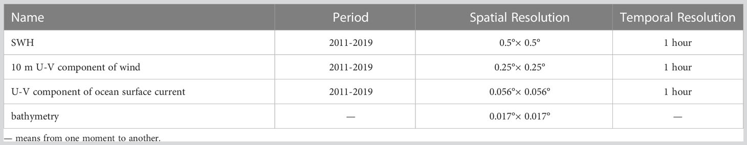
Table 1 The introduction of the data source.

(II) We perform ablation experiments on MF and the improved algorithm components of the PredRNN to reveal their roles.

(III) The input sequence length as an important parameter and the performance of the MF-PredRNN model under the high wave condition is also investigated.

2 Materials and methods

2.1 Study area and data

In this paper, the study area is 24°N~41°N and 118°E~132°E in the BYECS. The SWH is considered as the input sequence, the open boundary, and the target of the prediction. Important for the exchange of momentum and energy between the atmosphere and ocean (He et al., 2018), 10 m surface winds and ocean surface currents are added to the SWH prediction as upper boundaries. The SWH, 10 m surface winds and ocean surface current datasets are selected from a 1 Jan 2011 to 31 Dec 2019. The SWH and 10 m surface winds data are generated from a subset of ECMWF’s ERA5 reanalysis archive (www.ecmwf.int/en/forecasts/datasets/reanalysis-datasets/era5, Hersbach et al., 2020). The ocean surface currents are generated from numerical model ROMS (Yu et al., 2017 and Yu et al., 2020). The 1-min resolution bathymetry (Choi et al., 2002) that shows a strong statistical correlation with the SWH (Karmpadakis et al., 2020) is added to the SWH prediction. All the datasets are uniformly interpolated to 0.5°×0.5° spatial resolution, 1-hour temporal resolution using cubic spline interpolation. The processed datasets contain 87,648 hours temporally, 35 × 29 data matrix spatially, and consist of four different types of data. The processed dataset is divided into a training set (2011-2017), validation set (2018), and test set (2019), respectively. A mask matrix of the same size as the data matrix is set to distinguish land and sea, with land points set to 0 and sea points set to 1. The result is dot-multiplied by the mask matrix to eliminate the influence of land, and the points at the open and sea-land boundaries are removed in the loss function. Only the data within the open and sea-land boundaries are trained and tested.

2.2 MF-PredRNN algorithm

In this study, the PredRNN algorithm (c.f. Wang et al., 2022c) is applied to predict the spatiotemporal SWH, which mainly proposes these three improvements over the ConvLSTM algorithm:

1) Spatio-Temporal Memory Flow (STMF): The ST-LSTM recurrent unit and the double flow memory transition mechanism solve the problem of spatial feature loss from the top layer to the bottom layer of ConvLSTM. The ST-LSTM replaces the previous ConvLSTM as the basic recurrent unit of the stack structure, and the original memory cell $C$ and the new memory cell $M$ are used together for information transmission between the recurrent units. The following are the memory state transfer formulas in the recurrent unit ST-LSTM, where $g_t$, $i_t$ and $f_t$ used to calculate horizontal propagation memory cell $C$ represent the input modulation gate, input gate, and forget gate respectively, $g_t^{\prime }$, $i_t^{\prime }$ and $f_t^{\prime }$ used to calculate the memory cell $M$ which flows in the zigzag direction, $o_t$ represents the output gate, $t$ represents the time, $l$ represents the layer of the stack structure, $X_t$ represents the input data at time $t$.

$${\text{g}}_{\text{t}}=\tanh ({\text{W}}_{\text{xg}}*{\text{ X}}_{\text{t}}+{\text{W}}_{\text{hg}}{\text{* H}}_{\text{t}-1}^{\text{l}})$$

$${\text{i}}_{\text{t}}=\text{σ}({\text{W}}_{\text{xi}}*{\text{ X}}_{\text{t}}+{\text{W}}_{\text{hi}}*H_{\text{t}-1}^{\text{l}})$$

$${\text{f}}_{\text{t}}=\text{σ}({\text{W}}_{\text{xf}}*{\text{ X}}_{\text{t}}+{\text{W}}_{\text{hf}}{\text{* H}}_{\text{t}-1}^{\text{l}})$$

$${\text{C}}_{\text{t}}^{\text{l}}={\text{f}}_{\text{t}}\odot {\text{C}}_{\text{t}-1}^{\text{l}}+{\text{i}}_{\text{t}}\odot {\text{g}}_{\text{t}}$$

$${\text{g}}_{\text{t}}^{\prime }=\text{tanh}({\text{W}}_{\text{xg}}^{\prime }*{\text{X}}_{\text{t}}+{\text{W}}_{\text{mg}}*{\text{M}}_{\text{t}}^{\text{l}-1})$$

$${\text{i}}_{\text{t}}^{\prime }=\text{σ}({\text{W}}_{\text{xi}}^{\prime }*{\text{X}}_{\text{t}}+{\text{W}}_{mi}*{\text{M}}_{\text{t}}^{\text{l}-1})$$

$${\text{f}}_{\text{t}}^{\prime }=\text{σ}({\text{W}}_{\text{xf}}^{\prime }*{\text{X}}_{\text{t}}+{\text{W}}_{\text{mf}}*{\text{M}}_{\text{t}}^{\text{l}-1})$$

$${\text{M}}_{\text{t}}^{\text{l}}={\text{f}}_{\text{t}}^{\prime }\odot {\text{M}}_{\text{t}}^{\text{l}-1}+{\text{i}}_{\text{t}}^{\prime }\odot {\text{g}}_{\text{t}}^{\prime }$$

$${\text{o}}_{\text{t}}=\text{σ}({\text{W}}_{\text{xo}}*{\text{ X}}_{\text{t}}+{\text{W}}_{\text{ho}}{\text{* H}}_{\text{t}-1}^{\text{l}}+{\text{W}}_{\text{co}}*{\text{ C}}_{\text{t}}^{\text{l}}+{\text{W}}_{\text{mo}}{*\text{ M}}_{\text{t}}^{\text{l}})$$

$\begin{array}{ll}{\text{H}}_{\text{t}}^{\text{l}}={\text{o}}_{\text{t}}\odot \tanh ({\text{W}}_{1\times 1}*[{\text{C}}_{\text{t}}^{\text{l}},{\text{M}}_{\text{t}}^{\text{l}}])& (1)\end{array}$

2) Memory Decoupling (MD): The PredRNN algorithm adds the decoupling module for memory cells $C$ and $M$ to decouple long-term and short-term dynamics in transmission. The memory cell $C$, which focuses on long-term motion, is used to transmit the information from the previous moment, and the memory cell $M$, which focuses on short-term motion updated across all the layers and time steps, $M$ is used to transmit the spatiotemporal information from the previous layer and time step. The MD module separates the character of $C$ and $M$ to improve the information transmission. The equations are as follows,

$$∆C_t^l=W_{decouple}\times (i_t\odot g_t)$$

$$∆M_t^l=W_{decouple}\times (i_t^{\text{'}}\odot g_t^{\text{'}})$$

$\begin{array}{ll}{ℒ}_{decouple}=\sum _t\sum _l\sum _c\frac{\left|∆C_t^l,∆{M_t^l}_c\right|}{\left|\right|∆C_t^l|{|}_c.|\left|∆M_t^l\right|{|}_c}& (2)\end{array}$

where W_decouple represents the convolution shared by all recurrent units, L_decouple is the memory decoupling regularization. l, t and $c$ represent the layers, time steps, and channels, $\langle \Delta C_t^l,\Delta M_t^l\rangle$ represents the dot product of $\Delta C_t^l$ and $\Delta M_t^l$, $\Vert \Delta C_t^l\Vert$ represents the L2 norm of $\Delta C_t^l$.

3) Reverse Scheduled Sampling (RSS): To force the model to learn long-term dynamics from historical data, the PredRNN algorithm uses RSS as a new learning strategy that randomly hides true data as training proceeds.

Compared with ConvLSTM, the STMF module and MD module effectively use the long- and short-term dynamics and spatial correlation to improve prediction accuracy, and the RSS module promotes prediction accuracy by learning the long-term characteristics of historical data. Furthermore, the multiple channels of the PredRNN algorithm are used to combine multiple factors and historical SWH data to improve the long-term prediction accuracy of SWH.

2.3 Framework of the SWH prediction model

The framework of the data-driven SWH prediction model based on MF-PredRNN is shown in Figure 1. The input includes $W$, $X$, and SWH open boundary data, and its output is represented by $Y$, which is the predicted SWH data, where $W$ represents SWH data; $X$ represents multi factors (MF) including the U and V components of 10 m surface winds, the U and V components of ocean surface currents, and bathymetries. In the prediction process, the MF-PredRNN model is modified to a one-step prediction based on the recursive strategy. Taking the SWH prediction at time $t+1$ as an example: firstly, the historical SWH $(W_1,···,W_t)$ from time 1 to time $t$ and the MF from time 2 to time $t+1$ $(X_2,···,X_{t+1})$ are combined as the input to predict the SWH $Y_{t+1}$; secondly, the SWH at the open boundaries is imposed to correct the SWH $Y_{t+1}$ at open boundaries; finally, $Y_{t+1}$ and $X_{t+2}$ are added to the input data sequence to predict the SWH $Y_{t+2}$. This process cycles and iteratively predicts the SWH for 1-72h. In this study, we choose 12h as the input sequence length.

FIGURE 1

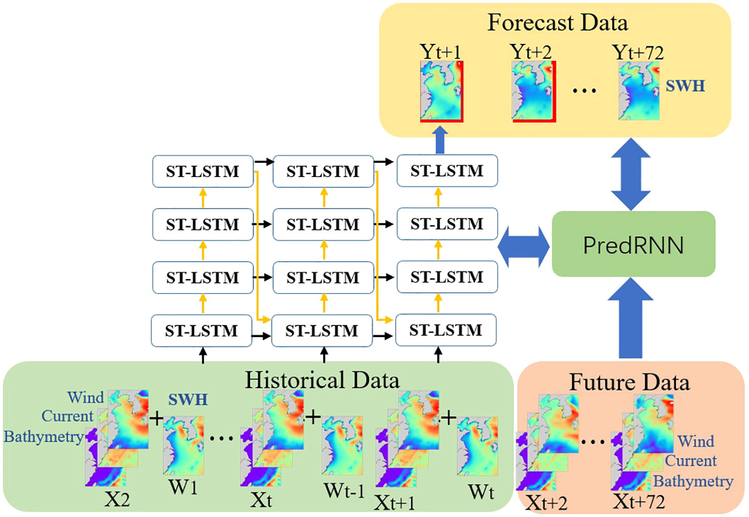
Figure 1 Framework of the MF-PredRNN-based SWH prediction model. The red lines show the imposed SWH at the open boundaries.

2.4 Evaluation indicators

Mean Absolute Error (MAE), Root Mean Squared Error (RMSE), and Mean Absolute Percentage Error (MAPE) are chosen to evaluate the error between predicted values and reanalysis data. MAE and MAPE measure the actual situation and the proportion of error, while RMSE reflects the dispersion between the predicted and reanalysis data. The Correlation Coefficient (CC) is used to measure the linear correlation between predicted values and reanalysis data.

3 Result

3.1 Results of prediction

As shown in Figure 2, The MAE of the MF-PredRNN predicted SWH relative to the ERA-5 reanalysis in the first 12 hours is within a small value (~0.2m) in most regions of the BYECS but increases with time. After 12 hours, the MAE accumulates and is mainly distributed in the Bohai Sea and the eastern Korean Peninsula with the MAE of ~0.4m. The MAE gradually stabilizes after 24 h and there is no significant difference between the 24h and 72h. According to our knowledge, the accumulation of MAE in the Bohai Sea and the eastern Korean Peninsula is likely caused by the complexity of the land-sea environment, and the sea area being surrounded by land. Although the dataset is separated by a land-sea mask, this also leads to eigenvalues in the offshore region.

FIGURE 2

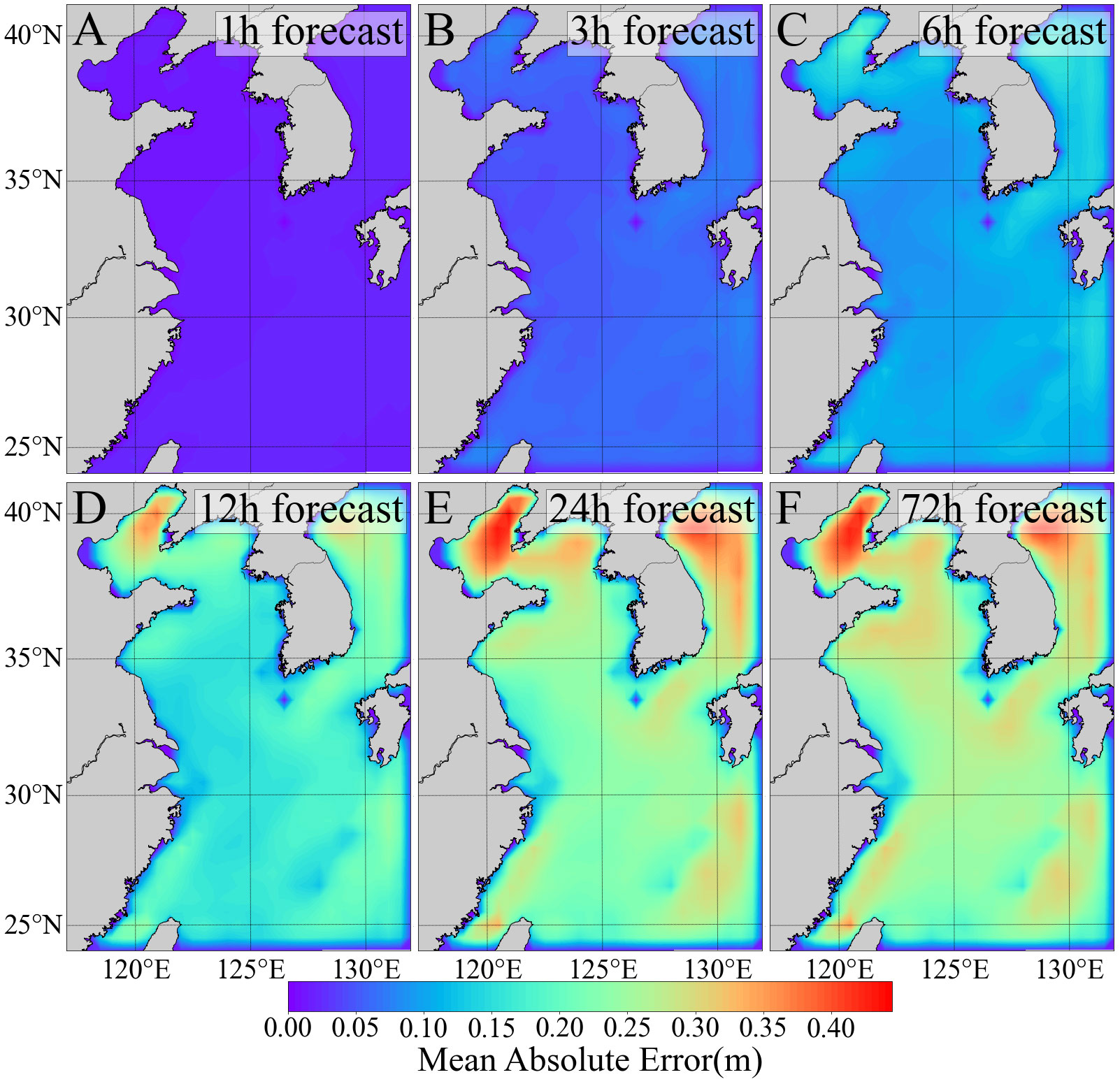
Figure 2 The MAE (A–F) between the MF-PredRNN predicted SWH and the ERA-5 reanalysis SWH for the 1-, 3-, 6-, 12-, 24- and 72-h respectively in the BYECS in 2019. Images for 24-72 h are omitted due to high similarity.

In addition, scatter plots and the other evaluation indicators such as RMSE, MAPE, and CC are used to evaluate the accuracy of the MF-PredRNN-based SWH prediction at different times (Figure 3). For the MF-PredRNN-based SWH prediction model, the CC decreases from 0.99 at 1h to 0.95 at 12h, 0.90 at 24h, and 0.87 at 72h, respectively, and the RMSE increases from 0.04m at 1h to 0.26m at 12h, 0.36m at 24h and 0.39m at 72h, respectively. The MAE at 24h is close to that at 72h, but the scatter plot of the 72h forecast is more dispersed compared to 24h, indicating that the error inevitably accumulates gradually. This is superior to the previous work. Due to the incomplete dynamic factors and the drawbacks of the ConvLSTM algorithm, the predictive time length of the ConvLSTM-based historical SWH-driven SWH prediction model is limited as the CC decreased from 0.99 at 1h to 0.83 at the 24h while the RMSE increased sharply from 0.20m at 1h to 0.60m at 24h (Zhou et al., 2021). With the introduction of winds, the ConvLSTM-based winds and historical SWH-driven SWH prediction model performs better. The RMSE increased from 0.09m at 1h to 0.49m at 24h (Song et al., 2022). By using a double-stage ConvLSTM network to incorporate future winds, the CC decreased from 0.95 on day 1 to 0.82 on day 3 (Ouyang et al., 2023). To our knowledge, the MAE, RMSE, MAPE, and CC of 1h, 6h, 12h, 24h, and 72h prediction show that the MF-PredRNN extends the effective prediction time length of SWH to 72h, and the accuracy of MF-PredRNN performs better than the existing spatiotemporal predictive learning ConvLSTM based 2D SWH prediction models (e.g., Zhou et al., 2021; Song et al., 2022; Ouyang et al., 2023), which take SWH or winds as model input.

FIGURE 3

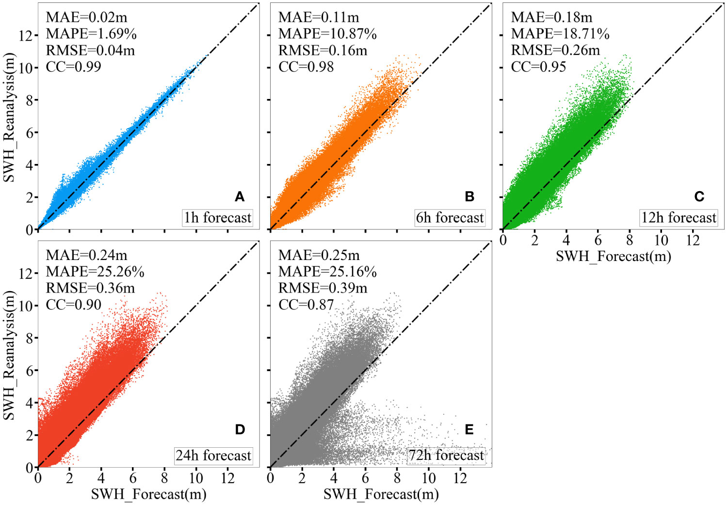
Figure 3 Two-dimensional scatter density plots (A–E) of the MF-PredRNN predicted SWH versus the ERA5 reanalysis data for the 1-, 6-, 12-, 24-, and 72-h respectively. The dashed line indicates that the predicted value is equal to the true value. The MAE, MAPE, RMSE, and CC are also calculated.

3.2 Comparison of the multivariate inputs and algorithms

To further explain the roles of MF and the PredRNN algorithm, a group of control experiments based on MF-PredRNN, MF-ConvLSTM, SF-PredRNN, and SF-ConvLSTM are conducted for 1-72h SWH prediction. SF refers to a single factor such as historical SWH, while MF refers to multi factors such as historical SWH, 10 m surface winds, surface currents, and bathymetries. MF-PredRNN, MF-ConvLSTM, SF-PredRNN, and SF-ConvLSTM have the same input sequence length. The difference between them is the factors labeled SF and MF and the algorithm labeled ConvLSTM and PredRNN. The experiments demonstrate the important role of both MF and PredRNN algorithm, as well as the error suppression of MF for long-term SWH prediction.

As shown in Figure 4, the MAE, RMSE, MAPE, and CC of PredRNN gradually stabilize after 24 hours. The spatially hourly averaged CC of the MF-PredRNN increased by 0.35, 0.62, and 0.44 compared with the MF-ConvLSTM, SF-PredRNN, and SF-ConvLSTM, and the spatially hourly averaged MAE decreased by 0.24m, 0.54m, and 1.45m.

FIGURE 4

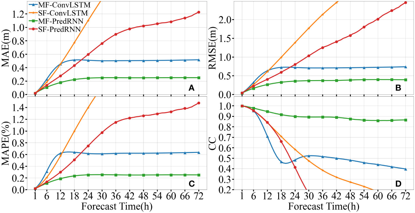
Figure 4 Comparison of spatially averaged MAE (A), RMSE (B), MAPE (C), and CC (D) among MF-PredRNN, SF-PredRNN, MF-ConvLSTM and SF-ConvLSTM over 1-72h hourly SWH prediction.

It is shown that both the PredRNN algorithm and MF can significantly improve the accuracy of SWH prediction. Moreover, the accuracy of PredRNN on the SWH prediction is generally better than the ConvLSTM, as the MF-PredRNN is superior to the MF-ConvLSTM in all indicators. Using the MF-PredRNN, the MAE, RMSE and MAPE reduced by 0.24m, 0.32m, and 35.12% respectively. At the same time, the CC increases by 0.35 compared to the MF-ConvLSTM in the 1-72h SWH prediction. Similarly, the SF-PredRNN is superior to the SF-ConvLSTM in MAE, RMSE, and MAPE indicators except for CC. The MF effectively prevents the rapid increase of the error in the long-term SWH prediction, much better compared to the single-factor calculation. There is no insignificant change between the MF and single-factor driven SWH during the first 12 hours of prediction, even for the ConvLSTM algorithm. The model driven by MF tends to be stable gradually after 18h, however, the error of the single factor driven SWH model increased rapidly. This leads to a gap in long-term SWH prediction. Compared to the SF-PredRNN, the mean MAE decreased by 0.54m, RMSE decreased by 0.89m, MAPE decreased by 70.39%, and CC increased by 0.62 in the 1-72h MF-PredRNN SWH prediction. Similarly, MF-ConvLSTM is superior to SF-ConvLSTM in all indicators. Above all, the MF-PredRNN algorithm provides the most accurate 1-72h SWH prediction.

4 Discussion

4.1 Input ablation experiments

The ablation experiments for MF are carried out to measure the role of each factor (Table 2). The factors include 10 m surface winds, ocean surface currents, bathymetries, historical SWH, and SWH as open boundaries. Our ablation experiments show that winds, as a dominant factor (Gao et al., 2021; Kim et al., 2022), can decrease the spatially hourly averaged MAE and RMSE by 0.13m and 0.28m, while the rest factors such as ocean surface currents, bathymetries and SWH as open boundaries only decrease the spatially hourly averaged MAE and RMSE by commonly around 0.02m and 0.04m (Table 2). In addition, the spatially averaged MAE of all experiments increases along with time (Figure 5). In the case of SWH prediction at 72h, relative to the MF-PredRNN control experiment, the spatially averaged MAE in the experiments of R-Wind, R-Current, R-Bathymetry, and R-Boundary increased by 0.22m, 0.05m, 0.04m, and 0.04m, respectively. In particular, the removal of winds induces about 5 times larger spatially averaged MAE growing with time than the other factors.

TABLE 2

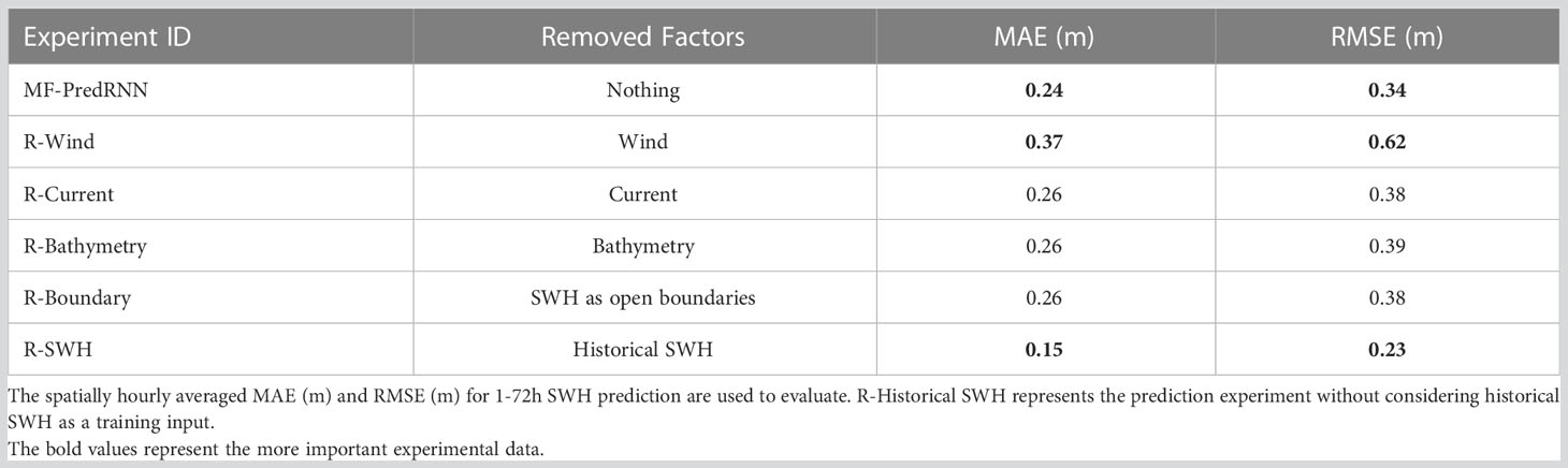
Table 2 The ablation experiments of MF-PredRNN-based SWH prediction model on multi factors.

FIGURE 5

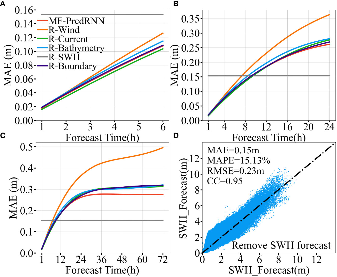
Figure 5 Comparison among ablation experiments of MF-PredRNN based SWH prediction model on multi factors. Figures (A-C) show the spatially averaged MAE (m) of 1-6h, 1-24h and 1-72h predicted SWH; Figure (D) shows the two-dimensional scatter density plots for the SWH prediction without the historical SWH; The legend shows the Experiment ID in Table 2. The grey solid line indicates the spatially averaged MAE for the R-SWH experiment.

The input ablation experiments show that MF has a greater impact on long-term prediction relative to short-term prediction. During the first 24 hours, the MAE of the MF-PredRNN experiment does not show much difference from other experiments with winds (<0.02m). But after 24 hours, the MAE of the MF-PredRNN with all factors control experiment is kept around 0.27m. That is slightly better than the MAE (0.32m) of experiments with winds and much better than the MAE of the R-Wind experiment (~0.50m).

The R-SWH experiment indicates that the historical SWH data has a positive impact on the accuracy of short-term prediction (Figures 5B, C). Due to the removal of the historical SWH, the error accumulation with time in the SWH prediction is eliminated (Figures 5A–C). The MAE value is stable at 0.15 (m) in both short- and long-term predictions. The RMSE, MAPE, and CC for the R-Historical SWH experiment are stabilized at 0.23m, 15.13%, and 0.95, respectively (Figure 5D). This is worse than the prediction with historical SWH in the first 10h, but better than it after 10h (Figures 3A–C, 5B–D). This illustrates the importance of historical SWH for short-term SWH prediction and MF for long-term SWH prediction. It is suggested that if the SWH in the next 1-10 hours is predicted by the MF-PredRNN model, while the SWH after 10 hours is predicted by the R-SWH model, the prediction error can be effectively suppressed.

4.2 Algorithm ablation experiments

In addition to the input ablation experiments, the algorithm ablation experiments are performed to evaluate the role of the improved components of the PredRNN including the memory decoupling (MD), reverse scheduled sampling (RSS), and spatiotemporal memory flow (STMF) compared to the ConvLSTM algorithm (Table 3). The roles of the MD and RSS are estimated by comparing the R-MD and R-RSS experiments with the MF-PredRNN control experiment. Since the STMF is encoded as a basic module in the MD module and cannot be removed separately, the role of STMF is verified by comparing the R-MD-RSS and MF-ConvLSTM experiments.

TABLE 3

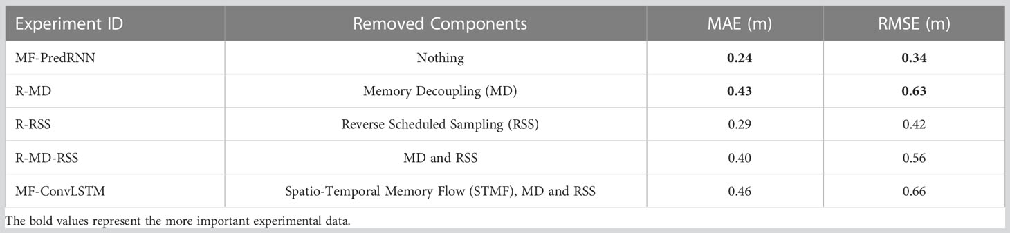
Table 3 Ablation experiments on algorithm components of PredRNN. Table legend: The spatially hourly averaged MAE (m) and RMSE (m) for 1-72h SWH prediction are used to evaluate.

The ablation experiments demonstrate the MD module is the key improved algorithmic component of PredRNN compared to ConvLSTM. Compared to the MF-PredRNN control experiment, the spatially hourly averaged MAE and RMSE of the 1-72h SWH prediction in the R-MD experiment dramatically increased by 0.19m and 0.29m respectively. In the R-RSS experiment, the MAE and RMSE increased slightly by 0.05m and 0.08m respectively due to the removal of the RSS module. Comparing the R-MD-RSS and MF-ConvLSTM experiments, the MAE and RMSE only increased by 0.06m and 0.10m respectively, showing the less important role of STMF. All of the three improved components of PredRNN have a positive impact on the accuracy of SWH prediction. Among them, the MAE and RMSE decreased by the MD module reached 0.19m and 0.29m, about 4-times larger than the MAE and RMSE decreased by the other two improvements including either STMF or RSS. It can be concluded that the MD module is the key component among the three improved components of the PredRNN compared to the ConvLSTM.

4.3 The sequence length of the input

Furthermore, the input sequence length of historical SWH is investigated as a sensitive parameter (Figure 6). The results show that the accuracy of the short-term prediction increases with increasing sequence length while the accuracy of the long-term prediction decreases and vice versa. When the input sequence length is 1h, i.e., only the spatial correlation information of SWH is retained while the temporal information is removed, the MAE of the 72 h prediction shows the smallest value (0.25m), meanwhile, the 1 h SWH prediction has the largest one (0.03m) compared to other input sequence length. This indicates that the spatial correlation information of SWH has a greater positive influence on the long-term prediction of SWH rather than on the short-term prediction. As the length of the input SWH sequence increased, the MAE of the short-term prediction gradually decreases but the long-term prediction gradually increases. When the input sequence length increases to 24h, the MAE of the 1-h prediction is the lowest (0.02m) and the 72-h prediction is the highest (0.45m) which indicates that the temporal information has a greater positive effect on the short-term prediction of SWH. Since the input sequence length is positively correlated with the accuracy of short-term prediction but negatively correlated with the accuracy of long-term prediction, we chose 12h as the input sequence length in this study to balance the accuracy of the short-term and long-term prediction.

FIGURE 6

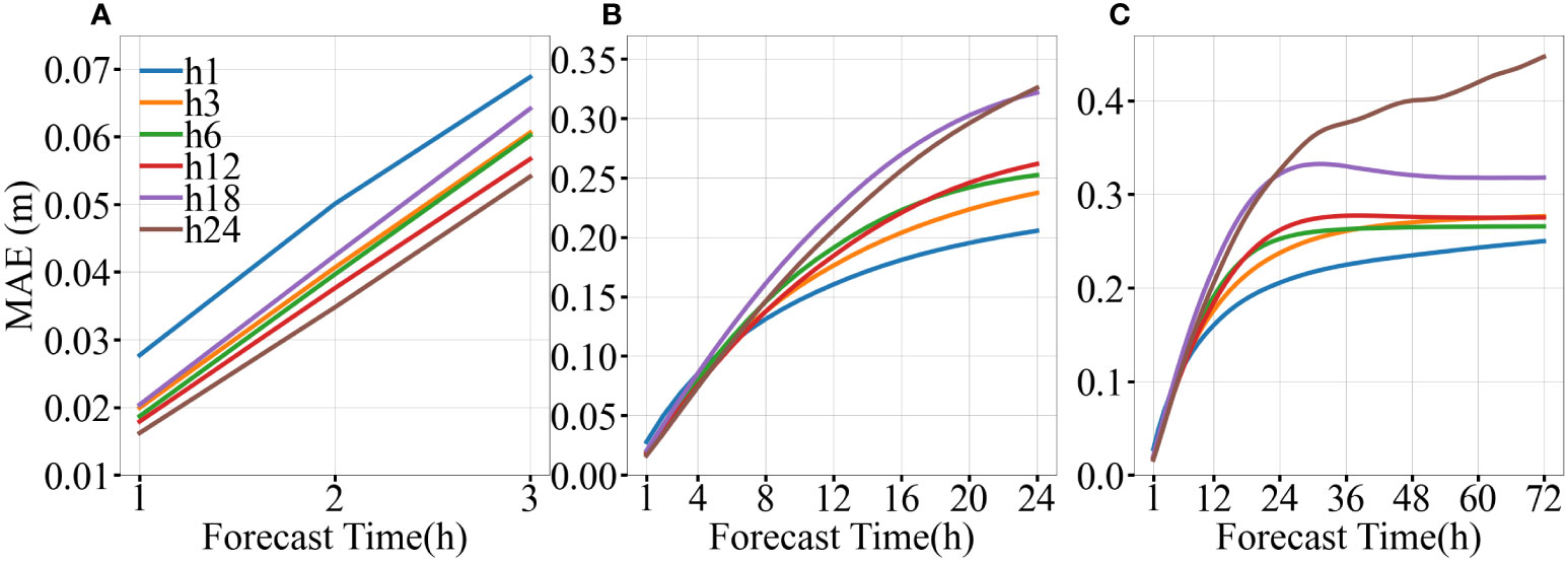
Figure 6 Time growth of MAE (h1, h3, h6, h12, h18, h24) for 1-3h (A), 1-24h (B), and 1-72h (C) SWH prediction with the input sequence length of historical SWH as 1, 3, 6, 12, 18 and 24 hours respectively.

4.4 Spatio-temporal SWH forecast for high wave

Under the high wave conditions of SWH >= 6 m, the MF-PredRNN can provide effective 6h spatiotemporal SWH prediction (Figures 7, 8). Under high wave conditions, the MAE became dramatically larger than the MAE under normal wave conditions (Figures 2, 7). The MAE in the first 6h is relatively smaller and well-distributed without significant error accumulation and is generally not higher than 1.20m (Figures 7A, B). In comparison, the MAE in the first 6h is less than 0.15m under normal wave conditions (Figure 2C). After 12 hours, the error accumulated rapidly and was mainly distributed in the Yellow Sea (Figure 7C). The MAE stabilized gradually after 24 hours. And there is no significant difference between the prediction of 24h and 72h (Figures 7D, E). In addition, the MAE of the 1h and 6h predictions are 0.10m and 0.73m, the RMSE are 0.14m and 0.89m, the MAPE is 1.50% and 10.24%, and the CC are 0.99 and 0.78 respectively (Figure 8). Without the historical SWH data as input, the MAE, RMSE, MAPE, and CC indicators are 0.70m, 0.86m, 9.98%, and 0.69, respectively, which are close to the prediction of 6h (Figures 8B, C).

FIGURE 7

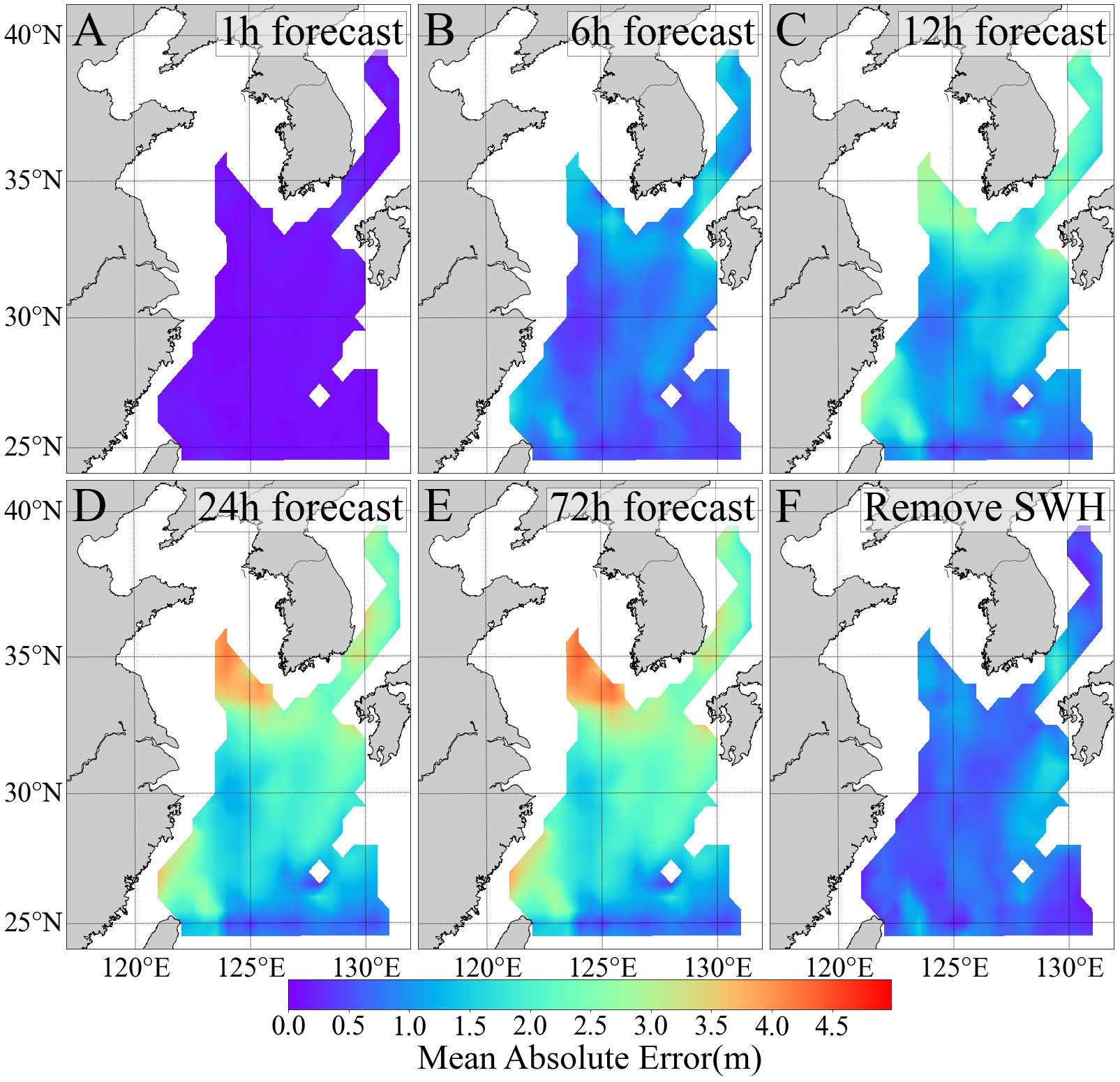
Figure 7 The MAE (A–E) between the MF-PredRNN predicted SWH and the ERA-5 reanalysis SWH for the 1-, 3-, 6-, 12-, 24- and 72-h respectively under high wave scenarios (SWH>=6m) in the BYECS in 2019. Images for 24-72 h are omitted due to high similarity. Figure (F) represents the MAE of prediction without the initial SWH data.

FIGURE 8

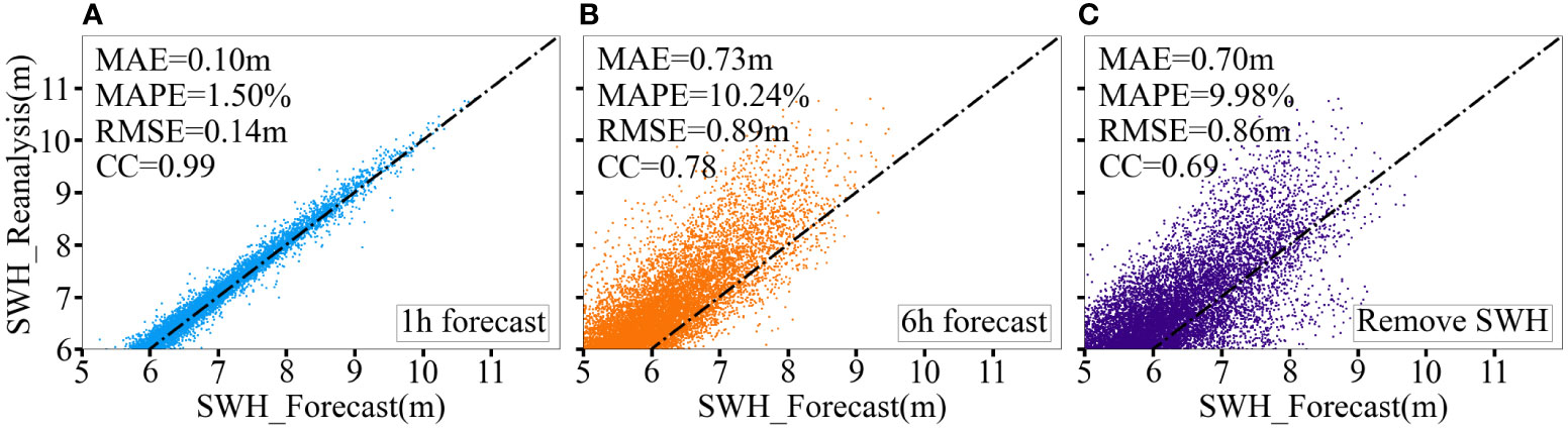
Figure 8 Two-dimensional scatter density plots (A, B) of the MF-PredRNN predicted SWH versus the ERA5 reanalysis data for the 1- and 6-h respectively under high wave scenarios (SWH>=6m); Figure (C) show the SWH prediction without the historical SWH. The dashed line indicates that the predicted value is equal to the true value. The MAE, MAPE, RMSE and CC were also calculated.

A group of control experiments based on MF-PredRNN, MF-ConvLSTM, SF-PredRNN, and SF-ConvLSTM are also conducted for a 1-12h SWH prediction to compare their accuracy under high wave conditions (Figure 9). The MF-PredRNN performs best in the 1-12h SWH prediction. The spatially hourly averaged CC of the MF-PredRNN increased by 0.21, 0.31, and 0.31 compared with the MF-ConvLSTM, SF-PredRNN, and SF-ConvLSTM respectively. The spatially hourly average MAE decreased by 1.62m, 0.34m, and 0.79m respectively. Here, the pairwise comparison shows that both the MF and the PredRNN algorithm also significantly improve the accuracy of SWH prediction under high wave conditions.

FIGURE 9

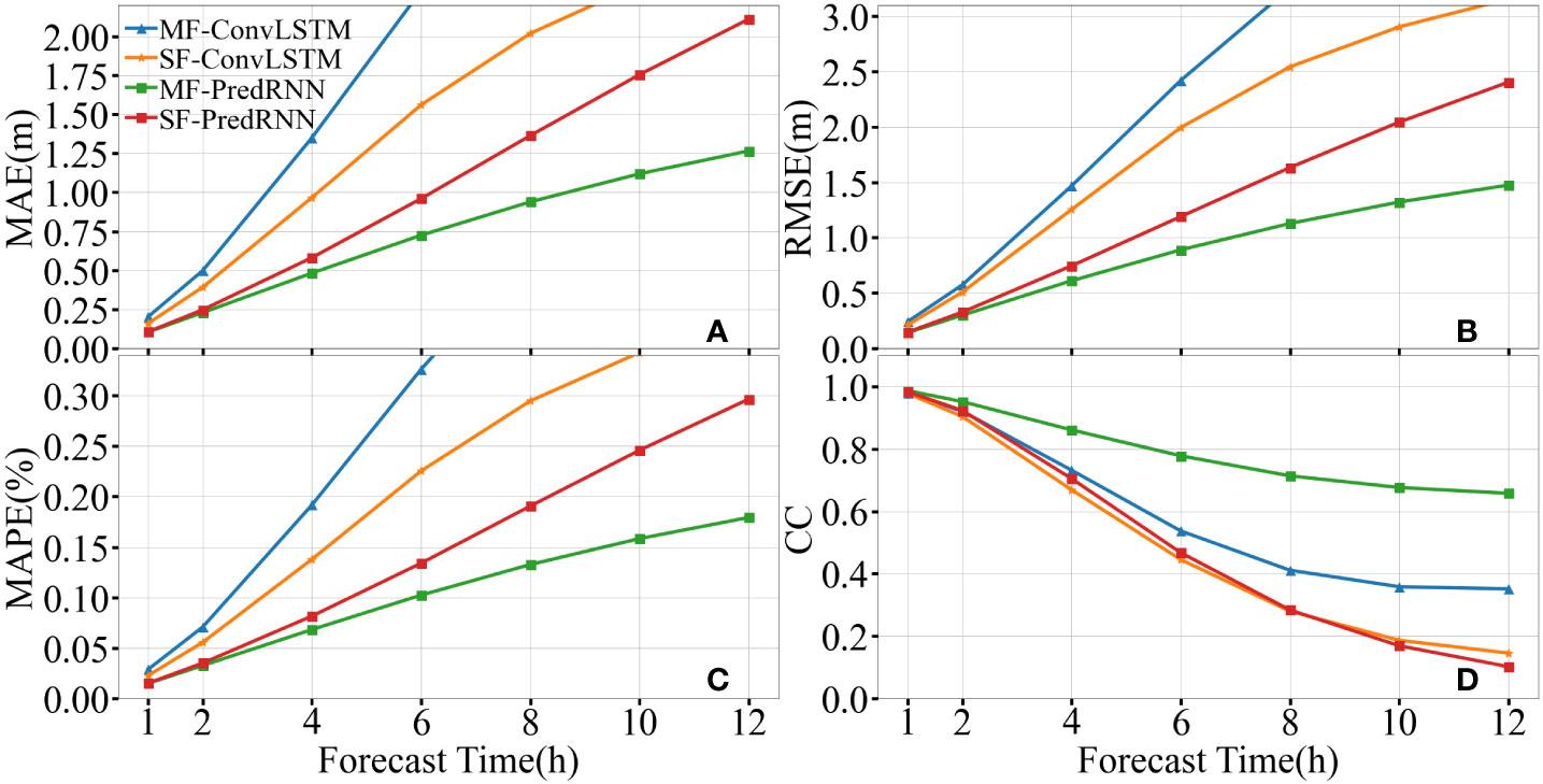
Figure 9 Comparison of spatially averaged MAE (A), RMSE (B), MAPE (C), and CC (D) among MF-PredRNN, SF-PredRNN, MF-ConvLSTM, and SF-ConvLSTM over 12h SWH hourly prediction under high wave scenarios (SWH>=6m).

5 Summary

In this study, an intelligent SWH prediction model based on the spatio-temporal predictive learning algorithm PredRNN and the MF including historical SWH, 10 m surface winds, ocean surface currents, bathymetries, and open boundaries is applied in the BYECS. The MF-PredRNN-based 2D SWH prediction model significantly improves the accuracy and extends the effective prediction time length, which can be used as a potential alternative to the numerical wave model. The correlation coefficients can reach 0.98, 0.90, and 0.87 for 6h, 24h, and 72h SWH prediction respectively. Under the high wave condition (SWH >= 6m), the MF-PredRNN-based SWH prediction model also provides effective 6h wave prediction.

The SWH prediction model based on MF-PredRNN performs much better than the SF-PredRNN, MF-ConvLSTM, and SF-ConvLSTM. Both the MF and PredRNN algorithms significantly improve the accuracy of the long-term SWH prediction. The ablation experiments have shown that winds are the most important factor among the MF. In addition, the removal of the historical SWH data from MF eliminates the accumulation of errors in the prediction process. The memory decoupling module is the key improved algorithmic component of PredRNN compared to ConvLSTM. As an important parameter, the input sequence length is chosen to be 12h to balance the short- and long-term prediction. As a future perspective to further improve the accuracy of wave prediction, the complexity of introducing other physical factors and mechanisms should be considered in the SWH spatiotemporal prediction.

Data availability statement

The original contributions presented in the study are included in the article. Further inquiries can be directed to the corresponding authors.

Author contributions

HC: Methodology, Formal analysis, Investigation, Writing – original draft; GL: Conceptualization, Supervision, Methodology, Investigation, Writing – review and editing, Resources, Funding acquisition; JH: Data Processing, Data Analysis, Resources; XG: Supervision, Data Analysis, Investigation, Writing – review and editing, Funding acquisition; YW: Data Analysis, Visualization, Validation, Funding acquisition; ZZ and DX: Data Management, Data Processing, Validation. All authors contributed to the article and approved the submitted version.

Funding

This study was funded by the Ministry of Science and Technology of the People’s Republic of China (No. 2019YFE0125000), Key R&D Program of Shandong Province, China (No. 2022CXGC020106), Pilot Project for Integrated Innovation of Science, Education, and Industry of Qilu University of Technology (Shandong Academy of Sciences) (No. 2022JBZ01-01), National Key R&D Program of China (No. 2020YFB0204804), State Key Laboratory of Biogeology and Environmental Geology, China University of Geosciences (No. GKZ22Y656) and Jinan Science and Technology Bureau (No. 202228034).

Conflict of interest

The authors declare that the research was conducted in the absence of any commercial or financial relationships that could be construed as a potential conflict of interest.

Publisher’s note

All claims expressed in this article are solely those of the authors and do not necessarily represent those of their affiliated organizations, or those of the publisher, the editors and the reviewers. Any product that may be evaluated in this article, or claim that may be made by its manufacturer, is not guaranteed or endorsed by the publisher.

References

Bahrpeyma F. (2021). Multistep ahead time series prediction. (Doctoral dissertation) (Dublin, Ireland: Dublin City University).

Google Scholar

Bai G., Wang Z., Zhu X., Feng Y. (2022). Development of a 2-d deep learning regional wave field forecast model based on convolutional neural network and the application in south China Sea. Appl. Ocean. Res. 18, 103012. doi: 10.1016/j.apor.2021.103012

CrossRef Full Text | Google Scholar

Bethel B. J., Dong C., Zhou S., Cao Y. (2021). Bidirectional modeling of surface winds and significant wave heights in the Caribbean. Sea. J. Mar. Sci. Eng. 9, 547. doi: 10.3390/jmse9050547

CrossRef Full Text | Google Scholar

Booij N., Ris R. C., Holthuijsen L. H. (1999). A third-generation wave model for coastal regions: 1. model description and validation. J. Geophys. Res. Oceans. 104, 7649–7666. doi: 10.1029/98JC02622

CrossRef Full Text | Google Scholar

Choi B. H., Kim K. O., Eum H. M. (2002). Digital bathymetric and topographic data for neighboring seas of Korea. J. Korean. Soc Coast. Ocean. Eng. 14, 41–50. Available at: https://koreascience.kr/article/JAKO200211920991563.pdf.

Google Scholar

Dong C., Xu G., Han G., Bethel B. J., Xie W., Zhou S. (2022). Recent developments in artificial intelligence in oceanography. Ocean Land Atmos. Res. 2022, 1–26. doi: 10.34133/2022/9870950

CrossRef Full Text | Google Scholar

Gao S., Huang J., Li Y., Liu G., Bi F., Bai Z. (2021). A forecasting model for wave heights based on a long short-term memory neural network. Acta Oceanol. Sin. 40, 62–69. doi: 10.1007/s13131-020-1680-3

CrossRef Full Text | Google Scholar

Gao Z., Shi X., Wang H., Zhu Y., Wang Y. B., Li M., et al. (2022). Earthformer: exploring space-time transformers for earth system forecasting. Adv. Neural Inf. Process. Syst. 35, 25390–25403. doi: 10.48550/arXiv.2207.05833

CrossRef Full Text | Google Scholar

Han L., Ji Q., Jia X., Liu Y., Han G., Lin X. (2022). Significant wave height prediction in the south China Sea based on the ConvLSTM algorithm. J. Mar. Sci. Eng. 10, 1683. doi: 10.3390/jmse10111683

CrossRef Full Text | Google Scholar

He H., Song J., Bai Y., Xu Y., Wang J., Bi F. (2018). Climate and extrema of ocean waves in the East China Sea. Sci. China. Earth. Sci. 61, 980–994. doi: 10.1007/s11430-017-9156-7

CrossRef Full Text | Google Scholar

Hersbach H., Bell B., Berrisford P., Hirahara S., Horányi A., Muñoz-Sabater J., et al. (2020). The ERA5 global reanalysis. Q. J. R. Meteorol. Soc 146, 1999–2049. doi: 10.1002/qj.3803

CrossRef Full Text | Google Scholar

Jörges C., Berkenbrink C., Stumpe B. (2021). Prediction and reconstruction of ocean wave heights based on bathymetric data using LSTM neural networks. Ocean. Eng. 232, 109046. doi: 10.1016/j.oceaneng.2021.109046

CrossRef Full Text | Google Scholar

Karmpadakis I., Swan C., Christou M. (2020). Assessment of wave height distributions using an extensive field database. Coast. Eng. 157, 103630. doi: 10.1016/j.coastaleng.2019.103630

CrossRef Full Text | Google Scholar

Kim J., Kim T., Yoo J., Ryu J. G., Do K., Kim J. (2022). STG-OceanWaveNet: spatio-temporal geographic information guided ocean wave prediction network. Ocean. Eng. 257, 111567. doi: 10.1016/j.oceaneng.2022.111576

CrossRef Full Text | Google Scholar

Laface V., Arena F. (2021). On correlation between wind and wave storms. J. Mar. Sci. Eng. 9, 1426. doi: 10.3390/jmse9121426

CrossRef Full Text | Google Scholar

Liang B., Gao H., Shao Z. (2019). Characteristics of global waves based on the third-generation wave model SWAN. Mar. Struct. 64, 35–53. doi: 10.1016/j.marstruc.2018.10.011

CrossRef Full Text | Google Scholar

Lin Z., Li M., Zheng Z., Cheng Y., Yuan C. (2020). Self-attention ConvLSTM for spatiotemporal prediction. P. AAAI. Conf. Artif. Intell. 34, 11531–11538. doi: 10.1609/aaai.v34i07.6819

CrossRef Full Text | Google Scholar

Mahjoobi J., Mosabbeb E. A. (2009). Prediction of significant wave height using regressive support vector machines. Ocean Eng. 36, 339–347. doi: 10.1016/j.oceaneng.2009.01.001

CrossRef Full Text | Google Scholar

Minuzzi F. C., Farina L. (2022). A deep learning approach to predict significant wave height using long short-term memory. Ocean. Model. 181, 102151. doi: 10.1016/j.ocemod.2022.102151

CrossRef Full Text | Google Scholar

Ning P., Zhang C., Zhang X., Jiang X. (2021). Short- to medium-term Sea surface height prediction in the bohai Sea using an optimized simple recurrent unit deep network. Front. Mar. Sci. 8. doi: 10.3389/fmars.2021.672280

CrossRef Full Text | Google Scholar

Ouyang L., Ling F., Li Y., Bai L., Luo J.-J. (2023). Wave forecast in the Atlantic ocean using a double-stage ConvLSTM network. Atmos. Ocean. Sci. Lett. 2023, 100347. doi: 10.1016/j.aosl.2023.100347

CrossRef Full Text | Google Scholar

Portillo Juan N., Negro Valdecantos V. (2022). Review of the application of artificial neural networks in ocean engineering. Ocean. Eng. 259, 111947. doi: 10.1016/j.oceaneng.2022.111947

CrossRef Full Text | Google Scholar

Shi X., Chen Z., Wang H., Yeung D.-Y., Wong W.-K., Woo W. C. (2015). Convolutional lstm network: a machine learning approach for precipitation nowcasting. Adv. Neural Inf. Process. Syst. 2015, 28. doi: 10.48550/arXiv.1506.04214

CrossRef Full Text | Google Scholar

Song T., Han R., Meng F., Wang J., Wei W., Peng S. (2022). A significant wave height prediction method based on deep learning combining the correlation between wind and wind waves. Front. Mar. Sci. 9. doi: 10.3389/fmars.2022.983007

PubMed Abstract | CrossRef Full Text | Google Scholar

Song T., Wang J., Huo J., Wei W., Han R., Xu D., et al. (2023). Prediction of significant wave height based on EEMD and deep learning. Front. Mar. Sci. 10. doi: 10.3389/fmars.2023.1089357

CrossRef Full Text | Google Scholar

Tang G., Du H., Hu X., Wang Y., Claramunt C., Men S. (2021) An EMD-PSO-LSSVM hybrid model for significant wave height prediction. Available at: https://os.copernicus.org/preprints/os-2021-2 (Accessed March 1, 2023).

Google Scholar

Tolman H. L. (2009) User manual and system documentation of wavewatch iii tm version 3.14. tech. note MMAB contribution 276. Available at: https://polar.ncep.noaa.gov/mmab/papers/tn276/MMAB_276.pdf.

Google Scholar

Villas Bôas A. B., Ardhuin F., Ayet A., Bourassa M. A., Brandt P., Chapron B., et al. (2019). Integrated observations of global surface winds, currents, and waves: requirements and challenges for the next decade. Front. Mar. Sci. 6. doi: 10.3389/fmars.2019.00425

CrossRef Full Text | Google Scholar

Wang L., Deng X., Ge P., Dong C., J. Bethel B., Yang L., et al. (2022b). CNN-BiLSTM-Attention model in forecasting wave height over south-East China seas. Cmc-comput. Mater. Con. 73, 2151–2168. doi: 10.32604/cmc.2022.027415

CrossRef Full Text | Google Scholar

Wang Y., Long M., Wang J., Gao Z., Yu P. ,. S. (2017). Predrnn: recurrent neural networks for predictive learning using spatiotemporal lstms. Adv. Neural Inf. Process. Syst. 30, 879–888. doi: 10.48550/arXiv.2103.09504.

CrossRef Full Text | Google Scholar

Wang G., Wang X., Wu X., Liu K., Qi Y., Sun C., et al. (2022a). A hybrid multivariate deep learning network for multistep ahead Sea level anomaly forecasting. J. Atmos. Ocean. Tech. 39, 285–301. doi: 10.1175/JTECH-D-21-0043.1

CrossRef Full Text | Google Scholar

Wang Y., Wu H., Zhang J., Gao Z., Wang J., Yu P. S., et al. (2022c). PredRNN: a recurrent neural network for spatiotemporal predictive learning. IEEE. T. Pattern Anal. 45 (2), 2208–2225. doi: 10.1109/TPAMI.2022.3165153

CrossRef Full Text | Google Scholar

Wei C.-C., Chang H.-C. (2021). Forecasting of typhoon-induced wind-wave by using convolutional deep learning on fused data of remote sensing and ground measurements. Sensors-basel. 21, 5234. doi: 10.3390/s21155234

PubMed Abstract | CrossRef Full Text | Google Scholar

Yu Y., Chen S.-H., Tseng Y.-H., Guo X., Shi J., Liu G., et al. (2020). Importance of diurnal forcing on the summer salinity variability in the East China Sea. J. Phys. Oceanogr. 50, 633–653. doi: 10.1175/JPO-D-19-0200.1

CrossRef Full Text | Google Scholar

Yu Y., Gao H., Shi J., Guo X., Liu G. (2017). Diurnal forcing induces variations in seasonal temperature and its rectification mechanism in the Eastern shelf seas of China. J. Geophys. Res. Oceans. 122, 9870–9888. doi: 10.1002/2017JC013473

CrossRef Full Text | Google Scholar

Zhou S., Xie W., Lu Y., Wang Y., Zhou Y., Hui N., et al. (2021). ConvLSTM-based wave forecasts in the south and East China seas. Front. Mar. Sci. 8. doi: 10.3389/fmars.2021.680079

CrossRef Full Text | Google Scholar