Bio-geo-optical modelling of natural waters

The color of natural waters – oceanic, coastal, and inland – is determined by the spectral absorption and scattering properties of dissolved and particulate water constituents. Remote sensing of aquatic ecosystems requires a comprehensive understanding of these inherent optical properties (IOPs), their interdependencies, and their impact on ocean (water) color, i.e., remote-sensing reflectance. We introduce a bio-geo-optical model for natural waters that includes revised spectral absorption and scattering parameterizations, based on a comprehensive analysis of precisely measured IOPs and water constituents. In addition, specific IOPs of the most significant phytoplankton groups are modeled and a system is proposed to represent the optical variability of phytoplankton diversity and community structures. The model provides a more accurate representation of the relationship between bio-geo-optical properties and can better capture optical variability across different water types. Based on the evaluation both using the training and independent testing data, our model demonstrates an accuracy of within ±5% for most component IOPs throughout the visible spectrum. We also discuss the potential of this model for radiative transfer simulations and building a comprehensive synthetic dataset especially for optically complex waters. Such datasets are the crucial basis for the development of satellite-based ocean (water) color algorithms and atmospheric correction methods. Our model reduces uncertainties in ocean color remote sensing by enhancing the distinction of optically active water constituents and provides a valuable tool for predicting the optical properties of natural waters across different water types.

1 Introduction

During the transfer of solar radiation through the atmosphere and water, light is absorbed and scattered, i.e., its energy is converted into another form such as heat and its direction of propagation is changed. In aquatic science, light absorption and scattering properties of a water body are also called inherent optical properties (IOPs) because they do not depend on the ambient light field in the medium. Interactions of sunlight in the upper water layer create the ocean (water) color, an apparent optical property (AOP), from which information about IOPs can be derived. Therefore, IOP modeling is used in the context with ocean color algorithm development. Spectral IOPs are fed into radiative transfer models, such as HydroLight (Mobley, 1994), to simulate remote-sensing reflectance, $R_{rs}$, and other interactions with (sun) light.

The color of natural waters contains a wealth of information about important constituents present in them, e.g., on primary production and pools of organic and inorganic carbon (Brewin et al., 2023). Therefore, ocean color is considered as an Essential Climate Variable (GCOS, 2011). The optically active components include phytoplankton, biogenic and minerogenic detritus, and chromophoric dissolved organic matter (CDOM). Interpreting the color information in terms of the concentrations and type of the different components requires the knowledge of the bio-geo-optical properties of the water body (Bricaud et al., 1998; Boss et al., 2001; Morel and Maritorena, 2001; Stavn and Richter, 2008). Optical remote sensing of aquatic ecosystems necessitates understanding the relationship between component concentrations and their IOPs, namely an “IOP model”, and how IOPs relate to relevant signals, such as the remote-sensing reflectance. However, the challenge of bio-geo-optical modeling of natural waters is that values of IOPs in optically complex waters, e.g., coastal waters, can vary by orders of magnitude (Twardowski et al., 2001; Mobley et al., 2004; Zheng et al., 2015; Hieronymi et al., 2017).

Water reflectance and other apparent optical properties can be calculated numerically and analytically under all light conditions (so-called forward modeling). To simplify this modeling, Morel and Prieur (1977) divided water bodies in nature into Case-1 and Case-2 types according to their optical properties. It is important to note that this binary classification does not imply high or low values of optical properties but instead represents a difference in the model assumptions (Mobley et al., 2004). For Case-1 waters, all optical properties (except pure water) are related to the phytoplankton biomass, which is parameterized by its total concentration of the pigment Chlorophyll a, [Chl], because it reflects the concentrations of most of the components due to the biological processes of phytoplankton (Morel and Maritorena, 2001). For Case-2 waters, omitting sea bottom effects, the IOPs are not only related to [Chl] but also to other components from terrigenous or benthic inputs (Prieur and Sathyendranath, 1981; Sathyendranath et al., 1989; Werdell et al., 2018). This leads to the fact that, assuming the IOPs of pure water are known, for Case-1 the bio-optical model requires only one variable, [Chl], which greatly simplifies the complexity of the model, while for Case-2 waters, the IOP model requires more inputs, which are not covariant. However, the global ocean does not always conform to the ideal Case-1 type, and Lee and Hu (2006) found that only about 60% of the ocean can be classified as such (depending on the used criterion), underscoring the complexity of a major part of natural waters. Another reason for the subdivision is the optimization of ocean color products from satellite remote sensing. As the boundaries of Case-1 and Case-2 are not always clear, the use of fuzzy-logic optical water type (OWT) classifications based on R_rs has been established in recent years, allowing suitable algorithms to be selected and seamless results to be produced (Moore et al., 2001; Moore et al., 2014; Mélin and Vantrepotte, 2015; Hieronymi et al., 2017; Jackson et al., 2017; Bi et al., 2019).

Component IOPs of Case-2 waters are usually treated separately, which is commonly referred to as a “Four-term” model (IOCCG, 2006 and references therein), including the four components pure water, CDOM, detritus, and phytoplankton as the four important components. However, one should note that, as per Case-2 definition, there are certainly other sources of IOPs, e.g., air bubbles (Stramski and Tegowski, 2001) or zooplankton (Basedow et al., 2019), which, however, are out of scope in this study (but any other components can be added easily to our model). The number “Four” here should be regarded as a “manageable number” as discussed in Stramski et al. (2001), which is a general concept of IOP assembly, and each component can be further separated into subcomponents based on how modelers understand the bio-geo-optical progress (Stramski et al., 2001, 2004). IOPs of pure water are typically parameterized as a function of wavelength, temperature, and salinity (Röttgers et al., 2016). The magnitude and spectral slope of CDOM vary significantly with molecular weight, source, and status of photobleaching of the relevant absorbing molecules (Röttgers and Doerffer, 2007; Helms et al., 2008), with the slope values usually present a lower variability in Case-2 waters (Babin et al., 2003b). Detritus refers to the non-living organic and inorganic matter in the water column. It can be challenging to differentiate between biogenic (from living organisms) and non-biogenic (minerogenic, from rocks and minerals) detritus due to their similar spectral shapes and non-additive properties (Stramski et al., 2001; Roesler and Boss, 2008; Röttgers et al., 2014a). However, by incorporating their individual concentrations in a forward bio-optical model, it is possible to understand their respective impacts on particulate IOPs across various water environments (Ramírez-Pérez et al., 2018; Lo Prejato et al., 2020). In Case-1 waters, it is reasonable to assume that detritus IOPs are more related to phytoplankton biomass due to its degradation, whereas in hydro-dynamically mixed shallow waters, they are more related to inorganic suspended matter concentrations. Phytoplankton IOPs show significant variability, with different phytoplankton groups exhibiting different spectral attributes (Bricaud et al., 1983; Sathyendranath et al., 1987; Hoepffner and Sathyendranath, 1991; Bracher et al., 2017). This variability can be attributed to the diversity of phytoplankton groups and species and their varying pigmentation, structural and morphological characteristics, which affect their light-interacting properties. This highlights the importance of considering the phytoplankton community composition when modeling IOPs and interpreting the results.

The main focus of building an IOP model is on the absolute values and spectral shapes (mostly from the ultra-violet to the near-infrared range) of the IOPs of individual components. The absolute values of the IOP components are related to their concentrations, and are typically described using mass-specific IOP coefficients. The spectral shape of mass-specific IOP is not dependent on the component concentrations in the water, and is instead a property of the component itself, determined by its biological, physical, and chemical properties. Some component IOP spectra are relatively simple, such as the absorption coefficient of CDOM, $a_g$ (where the subscript g stands for the methodologically more appropriate term gelbstoff), which exhibits a monotonically decreasing trend with wavelength, and can be well approximated by an exponential function in a certain wavelength range. Some are more complex, such as the absorption coefficient of phytoplankton, $a_{ph}$, which has a large peak in the blue-green spectral range and a narrower peak in the red spectral range. In larger absorbing phytoplankton particles, spectral scattering measurements (Bricaud et al., 1983; Roesler and Boss, 2003; Zhou et al., 2012) or simulations (Bernard et al., 2009; Organelli et al., 2018; Robertson Lain and Bernard, 2018) tend to show more peak-valley features. The feature is primarily due to the suppressions within absorption bands, which probably causes the inapplicability of assuming the scattering spectrum as a smooth power-law function (Babin et al., 2003a).

In satellite remote sensing of waters, there are many influencing factors, which produce partly similar features in the top-of-atmosphere radiance signal; these include the solar and observational angles, from the atmosphere especially the Rayleigh scattering from air molecules and aerosol influences, reflection effects at the water surface, and in the water column the IOPs of the different components. This can lead to ambiguities in the signal. Thus, accurate IOP modeling is important for the development of water algorithms, but also as a basis for atmospheric correction models. It allows the construction of large synthetic data sets without in situ measurements with unpredictable errors and possible data gaps (IOCCG, 2006). This is particularly important for the training of neural networks, which are used for about two decades for the inversion of remote sensing reflectance into IOPs, especially to solve the ambiguities for optically complex waters (Schiller and Doerffer, 1999; Doerffer and Schiller, 2000). However, due to simplification of bio-geo-optical properties, the simulations were based on several limiting assumptions and oversimplifications (Schiller and Doerffer, 1999; Doerffer and Schiller, 2007). To address these limitations, Hieronymi et al. (2017) developed an optical water type (OWT) classification and used a set of OWT-specific neural networks for a much wider range of applications including extremely absorbing or scattering waters; in addition, different phytoplankton groups were considered, but still with lacked confidence in the phytoplankton scattering coefficient due to the lack of observations. Note that it is important to consider phytoplankton community distribution in the forward modeling, since the phytoplankton diversity can result in varying cell sizes and pigment compositions, making the standard ocean color algorithm inapplicable across different water environments (Szeto et al., 2011; Bracher et al., 2017; IOCCG, 2019). For instance, coccolithophores exhibit IOPs and [Chl] that significantly differ from other types of algae, leading to distortion in the spectral band ratio (IOCCG, 2014). Detection of coccolithophores is often challenging, as they are usually only flagged when their brightness exceeds a certain threshold (Balch and Mitchell, 2023). To extend the dilemma further: in Case-2 waters, the relationships between water components are more intricate and often random (Woźniak and Dera, 2007). Thus, despite numerous in situ measurements since decades, a universal approach for all natural waters remains elusive (IOCCG, 2019). Hence, a radiative transfer modeling framework specific to algorithm development, such as the ONNS in-water algorithm (Hieronymi et al., 2017), is necessary. Given that, previous forward models based on deterministic functions, e.g., fixed parameters, may not capture all the variability, and utilizing reasonable random values can improve flexibility in simulations (IOCCG, 2006; Zheng et al., 2015; Loisel et al., 2023).

The aim of this study is to develop a bio-geo-optical IOP model that accurately reproduces IOPs from given component concentrations, and can effectively capture variations in optical properties across different water types. By conducting a detailed and comprehensive analysis of in situ data with high accuracy and a wide range, this model will provide guidance for feeding radiative transfer simulations such as HydroLight, which allows the creation of a new synthetic database. The findings of this study will enhance our understanding of the composition of the planktonic community and its impact on optical variability. Also, we will review the specific IOP assumptions, the spectral scattering in particular, on remote sensing reflectance. This will have important implications for ocean color remote sensing including boundary conditions for the atmospheric correction.

2 Fundamental concept of the IOP model

All symbols, abbreviations, and units used are presented in Table 1. IOPs are represented as the sum of light absorption or scattering by water molecules and by various dissolved and particulate constituents. Previous laboratory studies (Twardowski et al., 2001; Vaillancourt et al., 2004) have already demonstrated the separation of absorption and scattering based on observations. By adopting the widely accepted conceptual separation of IOPs (Mobley, 1994), the total absorption and total scattering coefficients can be formulated as:

TABLE 1

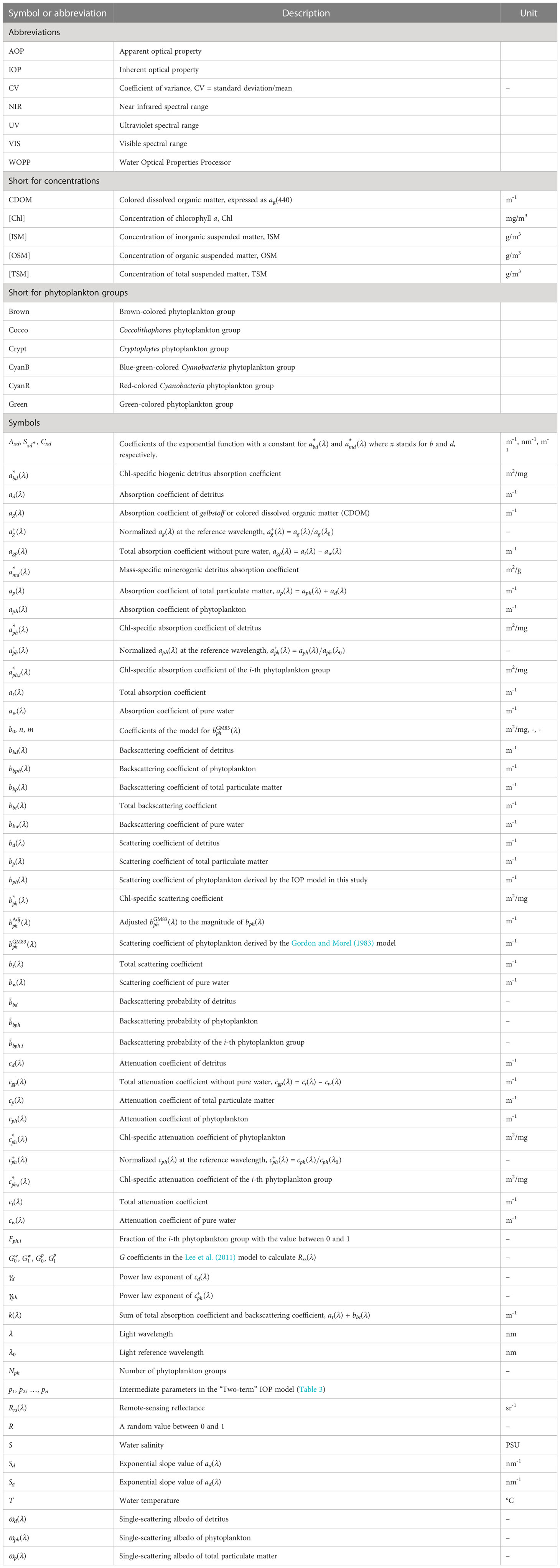
Table 1 List of symbols, abbreviations, definitions, and units.

$\begin{array}{ll}{a}_t(\lambda )=a_w(\lambda )+a_d(\lambda )+a_g(\lambda )+a_{ph}(\lambda )& (1)\end{array}$

and

$\begin{array}{ll}{b}_t(\lambda )=b_w(\lambda )+b_d(\lambda )+b_{ph}(\lambda ),& (2)\end{array}$

where $\lambda$ is the wavelength of light and the subscripts w, d, g, and ph stand for the four components: pure water, detritus, gelbstoff, and phytoplankton, respectively (no particulate scattering is usually attributed to the dissolved gelbstoff). However, if other components are important in a specific context, they can be added (Stramski et al., 2001). The attenuation coefficient is the sum of absorption and scattering, expressed as. The total particulate IOPs are represented as the sum of that of detritus and phytoplankton: $a_p(\lambda )=a_d(\lambda )+a_{ph}(\lambda )$ and $b_p(\lambda )=b_d(\lambda )+b_{ph}(\lambda )$. The subscript gp is used to represent the IOPs calculated as the sum of CDOM (gelbstoff) and total particulates.

The light backscattering coefficients of water components are determined by

$\begin{array}{ll}{b}_{bx}(\lambda )={\tilde{b}}_{bx}{b}_x(\lambda ),& (3)\end{array}$

where the subscript x represents different components (w, d, or ph), and ${\tilde{b}}_{bx}$ is the backscattering probability (or backscattering ratio). This ratio is the fraction of backward scattered light to total scattered light and is assumed to be constant, as no significant spectral changes have been observed (Twardowski et al., 2001; Vaillancourt et al., 2004). While ${\tilde{b}}_{bx}$ is normally calculated using volume scattering functions that describe the angular distribution of scattered light (Mobley, 1994; Harmel et al., 2021), in this study, fully radiative transfer simulations are not required as the focus is on forward modeling. Therefore, ${\tilde{b}}_{bx}$ is used as a simplification in the modeling work instead of the entire volume scattering function.

The single-scattering albedo, $\omega (\lambda )$, is the ratio of scattering to attenuation:

$\begin{array}{ll}{\omega }_x(\lambda )=b_x(\lambda )/c_x(\lambda ),& (4)\end{array}$

where the subscript x denotes total particle or individual components. $\omega (\lambda )$ is a dimensionless optical parameter combining $a(\lambda )$ and $b(\lambda )$ and is useful in optical modeling (Stramski et al., 2007). The total scattering coefficient $b(\lambda )$ can be easily determined if the shape of $c(\lambda )$ and $\omega (\lambda )$ are given.

2.1 The Four-term IOP model for complex waters

As mentioned in the introduction, the “Four-term” IOP model manages all components in Eqs. (1) and (2), separately. The IOPs of pure water are known and are not the subject of further modeling. The fundamental concepts of constructing IOPs of gelbstoff, detritus, and phytoplankton – so that it fits to our observational data – are illustrated in the following. The corresponding parameterizations, which we determined based on analyses of measured data, are given in section 3.2.

The absorption of gelbstoff in surface water, as a proxy of CDOM, can be expressed as:

$\begin{array}{ll}{a}_g(\lambda )=a_g({\lambda }_0)a_g^{+}(\lambda ),& (5)\end{array}$

where the reference wavelength, ${\lambda }_0$, is usually at 440 nm, and $a_g^{+}(\lambda )$ is the normalized $a_g(\lambda )$ at ${\lambda }_0$, which has typically a nearly exponential shape in the visible spectral range, which is most relevant in the ocean color context. To substitute the exponential function into Eq. (5), $a_g(\lambda )$ can be written as

$\begin{array}{ll}{a}_g(\lambda )=a_g({\lambda }_0)\exp (-S_g(\lambda -{\lambda }_0)),& (6)\end{array}$

where $S_g$ is the spectral slope estimated by nonlinear regression for a specific wavelength range, such as 350 to 500 nm (Babin et al., 2003b). The form of Eq. (6) has been widely accepted to compare the CDOM absorption coefficients across different systems but may have a risk when extrapolate to longer wavelengths, e.g., > 500 nm.

The absorption coefficient of detritus, $a_d(\lambda )$, is assumed to be controlled by both phytoplankton [Chl] and inorganic suspended matter, [ISM]. Following the concept of Ramírez-Pérez et al. (2018) and Lo Prejato et al. (2020), the absorption coefficient is constructed as:

$\begin{array}{ll}{a}_d(\lambda )=[\text{Chl}]a_{bd}^{*}(\lambda )+[\text{ISM}]a_{md}^{*}(\lambda ),& (7)\end{array}$

where $a_{bd}^{*}(\lambda )$ is the Chl-specific biogenic detritus absorption coefficient in the unit (m²/mg) and $a_{md}^{*}(\lambda )$ is the mass-specific minerogenic detritus in (m²/g). Note that the units of [Chl] and [ISM] are (mg/m³) and (g/m³), respectively.

The scattering of detritus is determined by the subtraction of its absorption from its attenuation:

$\begin{array}{ll}{b}_d(\lambda )=c_d(\lambda )-a_d(\lambda ).& (8)\end{array}$

The attenuation coefficient of detritus, $c_d(\lambda )$, is described as a power law function to avoid any negative values:

$\begin{array}{ll}{c}_d(\lambda )=c_d({\lambda }_0){(\frac{{\lambda }_0}{\lambda })}^{{\text{γ}}_d},& (9)\end{array}$

where the reference wavelength, ${\lambda }_0$, is often at 550 nm for its lower susceptibility to phytoplankton absorption, and ${\gamma }_d$ is the power law exponent. Using Eq. (9), we can determine the spectral shape of $c_d$. To ensure a positive scattering value obtained from Eq. (8), we calculate the magnitude of its attenuation based on the single-scattering albedo at ${\lambda }_0$, ${\omega }_d({\lambda }_0)$, which is a relative IOP parameter and can be empirically obtained. The magnitude of the spectrum, represented by $c_d({\lambda }_0)$, can be then calculated by:

$\begin{array}{ll}{c}_d({\lambda }_0)=\frac{a_d({\lambda }_0)}{1-{\omega }_d({\lambda }_0)}.& (10)\end{array}$

The absorption coefficient of phytoplankton is expressed as

$\begin{array}{ll}{a}_{ph}(\lambda )=[\text{Chl}]a_{ph}^{*}(\lambda ),& (11)\end{array}$

where $a_{ph}^{*}$ in (m²/mg) is the Chl-specific absorption coefficient, and [Chl] is commonly regarded as a proxy of the total phytoplankton concentration.

To capture the natural variability in phytoplankton IOPs due to the occurrence of different taxonomic groups, several phytoplankton groups with different optical properties and pigment compositions are considered. The Chl-specific absorption coefficient for phytoplankton is then expressed as:

$\begin{array}{ll}{a}_{ph}^{*}(\lambda )={\displaystyle {\sum }_{i=1}^{N_{ph}}{f}_{ph,i}{a}_{ph,i}^{*}(\lambda )},& (12)\end{array}$

where $f_{ph,i}$ is the fraction from 0 to 1 of each group in sum equal to 1, and $N_{ph}$ is the number of different groups used. $f_{ph,i}$ represents the proportionate contribution of each group to the total chlorophyll a concentration.

We define $a_{ph}^{+}(\lambda )$ as the normalized spectrum of phytoplankton absorption coefficient spectrum with respect to its value at the reference wavelength, which can be expressed as:

$\begin{array}{ll}{a}_{ph}^{+}(\lambda )=\frac{a_{ph}^{*}(\lambda )}{a_{ph}^{*}({\lambda }_0)}=\frac{a_{ph}(\lambda )}{a_{ph}({\lambda }_0)},& (13)\end{array}$

where ${\lambda }_0$ is the reference wavelength. Eq. (13) means one can obtain the spectral shape by any given phytoplankton absorption or specific absorption spectrum. Because we will afterwards obtain $a_{ph}(\lambda )$ once $a_{ph}({\lambda }_0)$ is provided. This value is deemed as the spectral magnitude and can be obtained based on its relationship with [Chl]. The relationship is often described using a power law function:

$\begin{array}{ll}{a}_{ph}({\lambda }_0)=A{[\text{Chl}]}^E,& (14)\end{array}$

where $A$ is the scale factor, and the power exponent, E, is often observed to be slightly below one in global data sets (Bricaud et al., 1998; Woźniak and Dera, 2007). $E$ represents the effects of pigment packaging and its interaction with phytoplankton cell size. Combining Eqs. (13) and (14), $a_{ph}(\lambda )$ of specific phytoplankton groups can be spectrally determined.

The reference wavelength ${\lambda }_0$ is often set at 443 nm (Bricaud et al., 2004). However, in this study, it was set at 676 nm, a wavelength where chlorophyll a is the dominating pigment absorption, and where $a_{ph}^{*}$ is assumed to be very similar between different taxonomic groups, while variations at 443 nm would be larger due to a different pigment composition in each group.

Having $c_{ph}(\lambda )=[\text{Chl}]c_{ph}^{*}(\lambda )$ , the Chl-specific attenuation coefficient of phytoplankton, $c_{ph}^{*}(\lambda )$, is expressed as the sum of those of the different groups:

$\begin{array}{ll}{c}_{ph}^{*}(\lambda )={\displaystyle {\sum }_{i=1}^{N_{ph}}{f}_{ph,i}{c}_{ph,i}^{*}(\lambda ).}& (15)\end{array}$

The phytoplankton Chl-specific scattering spectrum, $b_{ph}^{*}(\lambda )$, is then taken from the difference between those for attenuation and absorption:

$\begin{array}{ll}{b}_{ph}^{*}(\lambda )=c_{ph}^{*}(\lambda )-a_{ph}^{*}(\lambda ).& (16)\end{array}$

The backscattering of phytoplankton, $b_{bph}$, is calculated by multiplying $b_{ph}(\lambda )$ with the weighted sum of the backscattering probabilities of each phytoplankton group, ${\tilde{b}}_{bph}$, which is expressed as:

$\begin{array}{ll}{\tilde{b}}_{bph}={\displaystyle \sum f_{ph,i}{\tilde{b}}_{bph,i}}.& (17)\end{array}$

For phytoplankton groups for which $c_{ph}^{*}(\lambda )$ in Eq. (16) is unavailable, we will use ${\omega }_{ph}({\lambda }_0)$ and re-normalized $c_{ph}(\lambda )$ at the reference wavelength, i.e., $c_{ph}^{+}(\lambda )/c_{ph}^{+}({\lambda }_0)$, to determine $c_{ph}^{*}(\lambda )$:

$\begin{array}{ll}{c}_{ph}^{*}(\lambda )=\frac{c_{ph}^{+}(\lambda )}{c_{ph}^{+}({\lambda }_0)}\times \frac{a_{ph}^{*}({\lambda }_0)}{1-{\omega }_{ph}({\lambda }_0)},& (18)\end{array}$

where λ₀ is set at 676 nm likewise and ${\omega }_{ph}({\lambda }_0)$ can be empirically obtained from the measurements or literature for specific phytoplankton groups, which controls the magnitude of $c_{ph}^{*}(\lambda )$, and $c_{ph}^{+}(\lambda )$ only serves the spectral shape and can be assumed safely as a power law function ${({\lambda }_0/\lambda )}^{{\gamma }_{ph}}$ where the exponent ${\gamma }_{ph}$ determines the spectral slope. The power law function was also used to extrapolate $c_{ph}^{*}(\lambda )$ beyond the measured wavelength range.

2.2 The Two-term IOP model for phytoplankton dependence only

While the “Four-term” IOP model is highly adaptable, it may not be the most efficient option for simulating Case-1 waters, which make up the majority of the Earth’s oceans and are influenced by only two principal components: pure water and phytoplankton. Although the “Four-term” model can simulate these waters, it often requires more computational time and the gain in accuracy is small. To improve efficiency, we added a “Two-term” IOP model, as a supplement, by following the data synthesis process outlined in the IOCCG (2006), but using the setups for pure water and phytoplankton from the “Four-term” model (section 2.1) to mimic different phytoplankton groups. In the “Two-term” model, the fraction of phytoplankton groups from pico-phytoplankton to micro-phytoplankton is constrained by varying limits based on [Chl] levels. At low [Chl] levels, oceanic groups dominate, while other groups become mixed in as [Chl] increases (Brewin et al., 2010; Losa et al., 2017). However, in the “Four-term” model, there are no bounded limits as phytoplankton communities may be not correlated with [Chl] in optically complex water such as coastal and inland waters. The fraction setting is a preliminary biological limit that prevents unrealistic scenarios, but can be further refined with additional knowledge inputs.

3 Model development

3.1 Data sets

3.1.1 Fundamental data set for the model developing

The IOP model was developed using the “Hereon” data set collected by scientists of the Helmholtz-Zentrum Hereon in Germany (Röttgers et al., 2023). The comprehensive data set includes various water systems, including coast (the southern North Sea), river (the Elbe River), and ocean (the Atlantic Ocean), representing both Case-1 and Case-2 waters, which makes it suitable for building the IOP model. The data collection and processing methods of the coast and river parts (N=794) are detailed in Röttgers et al. (2023). However, the ocean part (N=40), which follows the same protocols, is not yet published. This part of data is primarily used for identifying and characterizing an oceanic phytoplankton group. Except that the [ISM] measurements are not available in the ocean part, the Hereon data set contains parameters of water constituents including [Chl], concentration of total suspended matter, [TSM], and concentration of organic suspended matter, [OSM]. [ISM] is calculated by subtracting [OSM] from [TSM]. The uncertainties of [TSM] and [OSM] measurements are given as the standard deviation using the method proposed in Röttgers et al. (2014b). Measurements of spectral IOPs, namely $c_{gp}(\lambda )$, $c_p(\lambda )$, $a_{gp}(\lambda )$, $a_p(\lambda )$, $a_g(\lambda )$, $a_d(\lambda )$, $a_{ph}(\lambda )$, $b_p(\lambda )$, and $b_{bp}(\lambda )$, are provided in the Hereon data.

3.1.2 External data sets for the model evaluation

Several external in situ data sets were considered to evaluate the IOP model. The “C22” data set, collected by Castagna et al. (2022), was obtained from turbid and eutrophicated Belgian inland and coastal waters, and it provides co-measured component concentrations, IOPs, and $R_{rs}$. The “HYPERMAQ”, gathered by Lavigne et al. (2022), consists of water samples from coastal and inland waters with co-measured component concentrations and IOPs. The “M17”, compiled by Mouw et al. (2017), contains samples from a four-year period in Lake Superior, a large freshwater lake that is dominated by CDOM. These data sets are utilized to test the “Four-term” IOP model with [Chl], [ISM], and $a_g(440)$ as inputs. Additionally, the “OC-CCI v3” data set by Valente et al. (2022), which is the third version of the collection for the ESA Ocean Colour-Climate Change Initiative (OC-CCI), was also utilized. This data set mainly comprises oceanic samples, including [Chl], $a_{ph}$, $a_{dg}$, $b_{bp}$, and $R_{rs}$, and was aggregated within ±2 nm of satellite bands. It was used to test the “Two-term” IOP model with [Chl] as input.

Furthermore, three simulated data sets were included to assess the coverage of optical properties. The “L23” database by Loisel et al. (2023), with a special focus on Case-1 waters, was synthesized following the process in IOCCG (2006), but its data distribution was constrained to fit the global distribution based on satellite products. The “CCRR” by Nechad et al. (2015), with a focus on Case-2 waters, was simulated based on in situ measurements collected in the ESA Coast Colour Round Robin project (see specifications in their Table 11). The “C2X” database by Hieronymi et al. (2016, 2017). addresses all natural waters, including Case-1 and extremely absorbing or scattering waters, though with some different IOP assumptions (see later discussion). Table 2 presents the sample number and the ranges of component concentrations.

TABLE 2

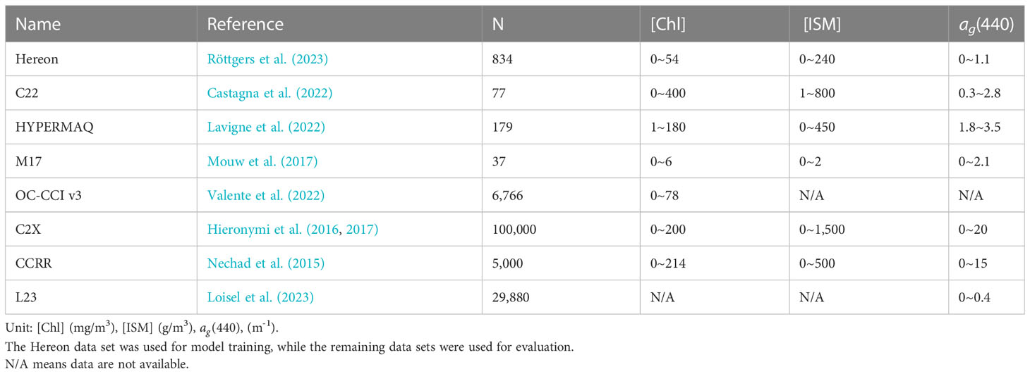
Table 2 The summary of IOP data sets used in this study.

3.2 Analysis of in situ data and parameterization of the IOP model

3.2.1 Pure water

The real part of the spectral refractive index of water, as well as water absorption and water scattering, are used as a function of wavelength, water temperature, and salinity. The calculation of pure water IOPs is based on the Water Optical Properties Processor (WOPP) (Röttgers et al., 2016 and references therein). The pure water light absorption coefficient in the UV/VIS part (< 510 nm) is taken from Mason et al. (2016).

3.2.2 CDOM

Figure 1 shows CDOM absorption spectra from the coastal, river, and oceanic waters from Hereon, C22, and M17. The spectral slope of most Case-2 waters exhibits relatively limited variation, with even more consistency observed in the turbid river data. However, variability in spectral slope is observed in Hereon – Ocean due to different sources of organic matters, photodegradation, precipitation, and microbial alteration of CDOM (Kieber et al., 2006; Helms et al., 2008). The distribution of $S_g$ in the data set is consistent with previous reports in European coastal waters (Babin et al., 2003b) of 0.0176 ± 0.002 nm^-1, and the shape is comparable to the determination in the Ligurian Sea (Ramírez-Pérez et al., 2018).

FIGURE 1

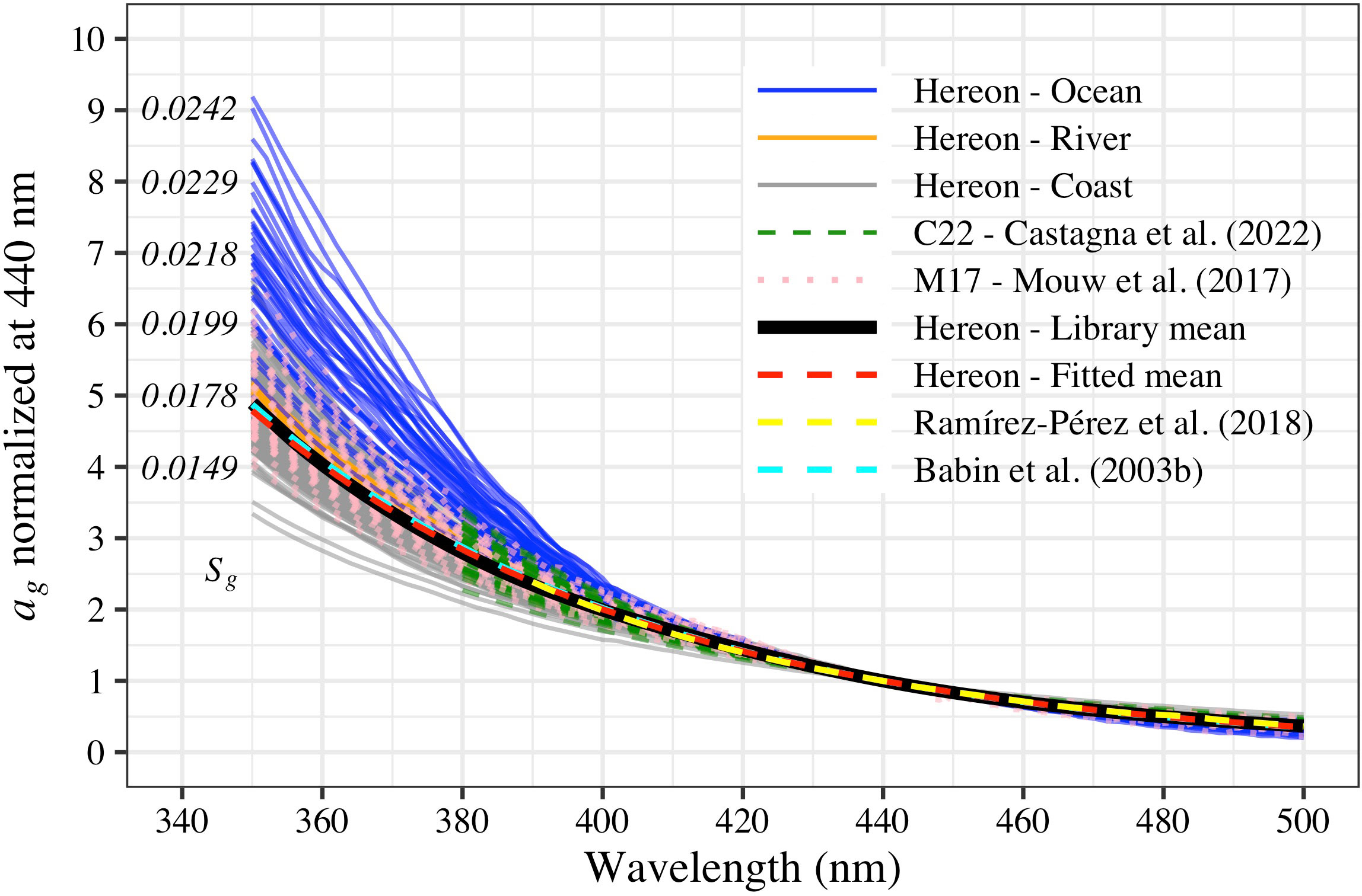
Figure 1 Normalized CDOM absorption spectra, $a_g^{+}(\lambda )$, from data sets Hereon (grouped into ocean, river, and coast), C22 (Castagna et al., 2022), and M17 (Mouw et al., 2017), as well as from modeled spectra by Ramírez-Pérez et al. (2018) and Babin et al. (2003b). The red dashed line represents the fitted $a_g^{+}(\lambda )$ spectrum based on the exponential function, Eq. (6), with a mean S_g value of 0.0174 nm^-1. The black solid line indicates the mean spectrum of the $a_g^{+}(\lambda )$ library in the IOP model (see text). Spectral slopes for a_g on the left.

Initially, we used the exponential function, Eq. (6), to fit $a_g(\lambda )$ measurements from the Hereon data within the 350~500 nm range. This yielded a mean $S_g$ value of 0.0174 ± 0.0014 nm^-1, with fitted slope values varying in a narrow range. However, using this mean slope caused a discrepancy between modeled $a_g(\lambda )$ values and measured values at longer wavelengths, with the modeled $a_g(560)$ by Eq. (6) being approximately 20% lower than the real measurements on average. To address this issue, we identified a normalized spectrum from measurements with the nearest $S_g$ values (see black solid line in Figure 1). To account for the variability of the $a_g(\lambda )$ shape in the UV, we constrained the percentage difference of $S_g$ between the fitted mean value to be less than 0.1%, resulting in a library of twelve $a_g^{+}(\lambda )$ spectra (not shown). Such random selection of $a_g^{+}(\lambda )$ exhibits deviations of 0.7685 and 0.0543 at 300 and 350 nm, respectively. Finally, in the “Four-term” IOP model, Eq. (5) will be used to model $a_g(\lambda )$ by providing $a_g(440)$ and randomly selecting an $a_g^{+}(\lambda )$ spectrum from the library.

3.2.3 Detritus

To determine $a_{bd}^{*}(\lambda )$ and $a_{md}^{*}(\lambda )$ in Eq. (7), we formulated a linear matrix equation at each wavelength:

$\begin{array}{ll}\left[\begin{array}{cc}{[\text{ISM}]}_1& {[\text{Chl}]}_1\\ {[\text{ISM}]}_2& {[\text{Chl}]}_2\\ \cdots & \cdots \\ {[\text{ISM}]}_n& {[\text{Chl}]}_n\end{array}\right]\times {[a_{md}^{*}({\lambda }_i), a_{bd}^{*}({\lambda }_i)]}^{\text{T}}=\left[\begin{array}{c}{a}_d{({\lambda }_i)}_1\\ a_d{({\lambda }_i)}_2\\ \cdots \\ a_d{({\lambda }_i)}_n\end{array}\right],& (19)\end{array}$

where n denotes the number of samples used to solve the equation matrix, i denotes the wavelength number, and here T denotes the transpose sign. This equation satisfies the condition $a_{md}^{*}({\lambda }_i)>0$ and $a_{bd}^{*}({\lambda }_i)>0$.

To reduce noise effects in the solution of Eq. (19), we applied constraints to the Hereon data for [Chl], [ISM], and $a_d(\lambda )$ measurements. Any detritus absorption spectra that showed remnants of pigment absorption were discarded. The coefficients of variation (CV) of each component concentration were calculated as the ratio of its standard deviation to the mean value (Röttgers et al., 2014b). To select for accurate, detritus dominated measurements, we applied the following constraints: CV(TSM) ≤ 0.3, CV(OSM) ≤ 0.3, and the proportion of detritus of total particle absorption, $a_d(550)/a_p(550)\ge 0.5$. Note that the values used here for constraints are arbitrary to ensure sufficient samples to solve Eq. (19). As a result, there were n = 80 data combinations in Eq. (19). To avoid biased results, we used a “Markov-chain” Monte Carlo algorithm by Meersche et al. (2009) to solve Eq. (19). 3,000 iterations were used as suggested by this algorithm. The results are presented as points in Figures 2A, B. The variability of $a_{bd}^{*}(\lambda )$ is higher than that of $a_{md}^{*}(\lambda )$, and the separation of biogenic and minerogenic components has a significant impact on the shape of $a_d(\lambda )$, depending on the ratio of [Chl] and [ISM]. Even though we conducted quality control on $a_d(\lambda )$, a slight peak around 676 nm still appeared in the determined $a_{bd}^{*}(\lambda )$, as observed in a similar study by Ramírez-Pérez et al. (2018). This peak may be due to imperfect bleaching of pigments, so we excluded the region around 676 nm for the non-linear regression of $a_{bd}^{*}(\lambda )$.

FIGURE 2

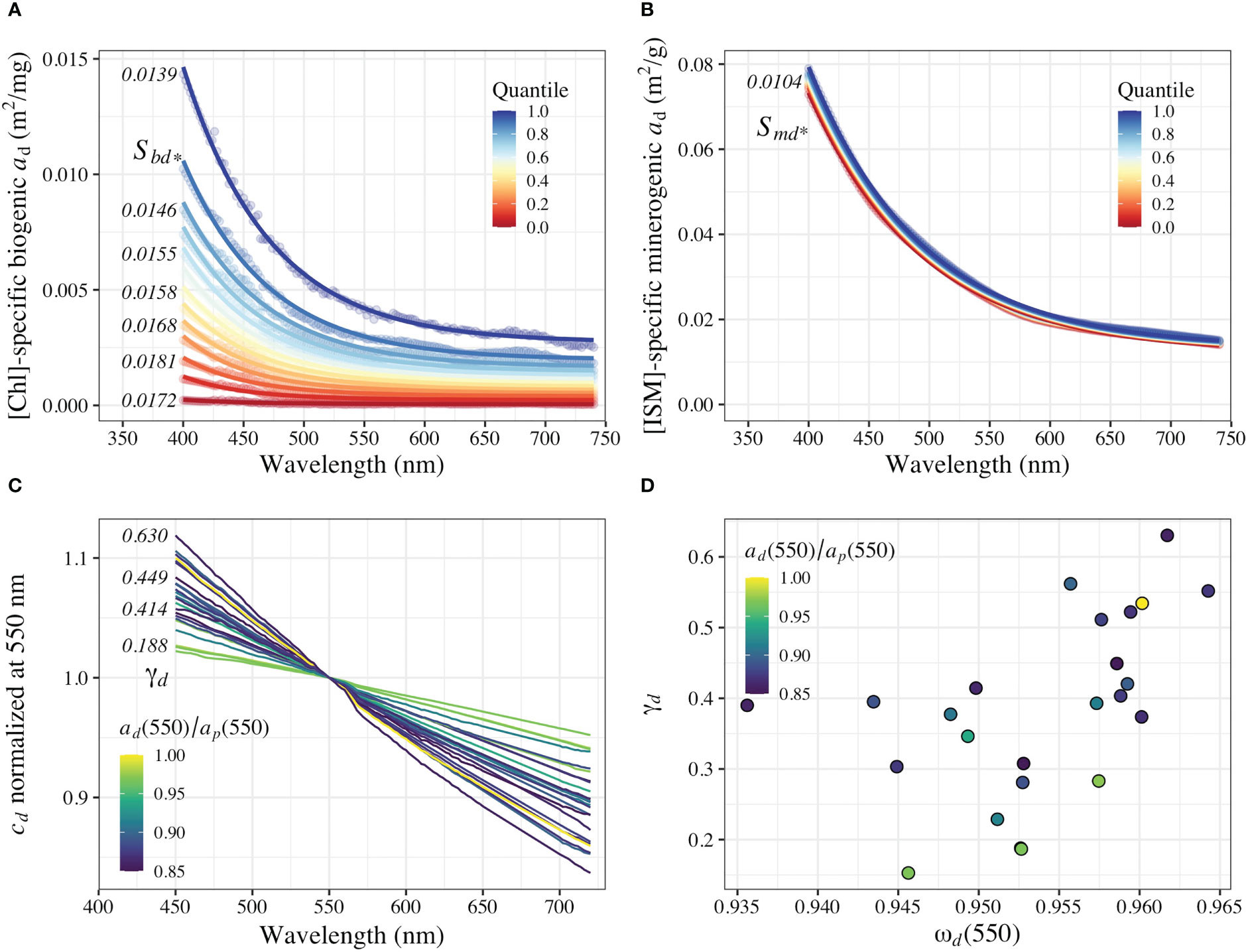
Figure 2 Spectral coefficients of detritus. (A) Chl-specific biogenic detritus absorption, m²/mg. (B) ISM-specific minerogenic detritus absorption, m²/g. (C) Normalized particle attenuation spectra at 550 nm. Note that the Y-axis does not start from the origin. (D) Scatter plot of ω_d (550) and γ_d (550). Determined on varying quantiles, points fitted in exponential functions with constant. Normalized attenuation spectra fitted based on power law function. Spectral slopes for $a_{bd}^{*}$, $a_{md}^{*}$, and c_d on the left of panels (A–C).

We employed an exponential function with a constant to fit $a_{bd}^{*}(\lambda )$ and $a_{md}^{*}(\lambda )$ as there were non-zero signals in the near infrared (Röttgers et al., 2014a). This function is given by:

$\begin{array}{ll}{a}_{xd}^{*}(\lambda )=A_{xd}\exp (-S_{x{d}^{*}}(\lambda -{\lambda }_0))+C_{xd},& (20)\end{array}$

where the subscript x denotes biogenic and minerogenic detritus as b and m, respectively, and ${\lambda }_0$ represents the reference wavelength at 550 nm. We tested the function with and without a constant $C_{xd}$ and found that including the constant yielded better results, which is consistent with the findings in Woźniak and Dera (2007). The Meersche et al. (2009) method resulted in $a_{xd}^{*}({\lambda }_i)$ as a normal distribution per wavelength, so we performed an exponential fit at different quantiles, ranging from 0 to 1, of $a_{bd}^{*}(\lambda )$ and $a_{md}^{*}(\lambda )$. The quantile of 0.5 indicates the maximum of the distribution, representing the average condition for the selected data. For this average condition, the coefficients are $A_{bd}$ = 0.0004 m^-1, $S_{b{d}^{*}}$ = 0.0158 nm^-1, $C_{bd}$ = 0.001 m^-1, $A_{md}$ = 0.0135 m^-1, $S_{m{d}^{*}}$ = 0.0104 nm^-1, and $C_{md}$ = 0.0122 m^-1. The coefficients of Eq. (20) for other quantiles in the Hereon data set are listed in the Supplementary Material (Table A3). Although higher quantiles may suggest a higher organic composition of particles, we found no significant correlation and therefore this requires further investigation before being used.

Measurement of attenuation and scattering of detritus alone are technically not feasible. Therefore, we began by analyzing total particles and selecting again detritus-dominated samples to represent the IOPs of detritus. Subsequently, we used these IOPs to parameterize the spectral slope of attenuation, ${\gamma }_d$, and the single-scattering albedo of detritus at the reference wavelength, ${\omega }_d({\lambda }_0)$, in Eqs. (9) and (10), respectively. We applied two constraints to the training data: 1) $a_d(550)/a_p(550)\ge 0.85$ and 2) only surface samples (water depth ≤ 12 m). Based on these criteria, we obtained 24 samples where we assumed that the $c_p(\lambda )$ spectra represented $c_d(\lambda )$. The distribution of ${\gamma }_d$ and ${\omega }_d(550)$ for these samples are shown in Figures 2C, D, respectively. The mean value of ${\gamma }_d$ is 0.3835 ± 0.1277 nm^-1, which follows a normal distribution function. As ${\gamma }_d$ decreases, the spectrum gradually flattens, indicating that detritus increasingly dominates, which has been reported by other studies too (Voss, 1992; Boss et al., 2001; Twardowski et al., 2001; Neukermans et al., 2012). To satisfy a normal distribution, we re-transformed the single-scattering albedo of detritus, ${\omega }_d(550)$, using ${\log }_{10}(1-{\omega }_d(550))$. The resulting mean value of transformed ${\omega }_d(550)$ is –1.3390 ± 0.0618 (mean of 0.9542 on its original scale). The determined ${\omega }_d(\lambda )$ spectrum (not shown) is comparable to laboratory measurements of most terrigenous particles (Stramski et al., 2007). Finally, we set the backscattering probability of detritus, ${\tilde{b}}_{bd}$, as 0.0216 based on these measurements.

To summarize, the “Four-term” IOP model follows a process where a quantile value between 0 and 1 is randomly chosen from the fitting results to determine $a_{bd}^{*}(\lambda )$ and $a_{md}^{*}(\lambda )$ using Eq. (20). Next, $a_d(\lambda )$ is calculated based on [Chl] and [ISM] using Eq. (7). ${\gamma }_d$ and ${\omega }_d(550)$ are randomly generated from normal distributions based on their statistical parameters to determine $c_d(\lambda )$. Finally, $b_d(\lambda )$ is obtained using Eq. (8), and $b_{bd}(\lambda )$ is calculated by multiplying $b_d(\lambda )$ with ${\tilde{b}}_{bd}$. One should note that the random terms used for detritus IOPs are derived from the Hereon statistics and are already representative. However, they can be adjusted to other specific environments, which is relatively more convenient compared to other models that require the replacement of entirely new specific-IOPs.

3.2.4 Phytoplankton

The relationships between [Chl] and $a_{ph}(676)$ from the Hereon data is shown in Figure 3A, after excluding outliers (i.e., water depth > 12 m and ten samples with obvious $a_{ph}$ noise). A power law function, Eq. (14), was initially used to fit the data. However, for lower [Chl] values (≤ 1 mg/m³), we found that a linear relationship (E = 1) was more appropriate. Therefore, $a_{ph}(676)$ can be expressed using a hybrid function:

FIGURE 3

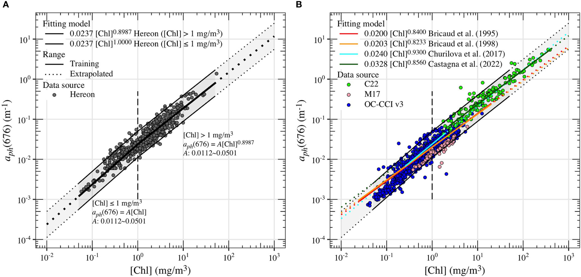
Figure 3 Relationship between [Chl] and a_ph (676) on the log₁₀ scale with different regression curves from previous studies and the Hereon data. The solid lines denote the training data range and the dashed lines are extrapolated. Points in panel (A) are for the Hereon data and panel (B) for the external data sets.

$\begin{array}{ll}{a}_{ph}(676)=\{\begin{array}{c}0.0237{[\text{Chl}]}^{1.0000}, [\text{Chl}]\le 1 \text{mg}/{\text{m}}^3\\ 0.0237{[\text{Chl}]}^{0.8987}, [\text{Chl}]>1 \text{mg}/{\text{m}}^3\end{array}.& (21)\end{array}$

To account for natural variation, the equation allows a deviation within ±20% of the $A$ coefficient (i.e., 0.0112~0.0501) (Bricaud et al., 1995). Figure 3B demonstrates that this range agrees well with other data sets and other fitting models (Bricaud et al., 1995; Bricaud et al., 1998; Churilova et al., 2017; Castagna et al., 2022).

To capture the optical features of phytoplankton diversity, we selected spectral properties of seven different phytoplankton groups. Five of these groups represent the essence of distinguishable phytoplankton absorption spectra of algal cultures determined in preliminary work by the authors (Xi et al., 2015; Hieronymi et al., 2017; Xi et al., 2017) and include: (1) a brown group (Heterokontophyta [including diatoms], Dinophyta, and Haptophyta), (2) a green group (Chlorophyta), (3) the Cryptophyceae; (4) a blue-green-colored Cyanobacteria and (5) a red-colored Cyanobacteria. In addition, two other groups were considered: (6) “Phytoplankton Case-1” for oligotrophic Case-1 waters and (7) a group representing Coccolithophores. The “Phytoplankton Case-1” group shall represent a small-sized group of widely distributed oceanic phytoplankton (Synechococcus and Prochlorococcus), that play an important role in global primary production. The corresponding IOP data for this group were collected in the tropical-subtropical North Atlantic Ocean (RV Sonne, SO287, 12/2021-01/2022) following the same protocol as in Röttgers et al. (2023). Coccolithophores are marine group that are abundant in temperate zones and exhibit strong particulate scattering, which can dominate ocean color properties. Without blooms, their $b_{bph}$ typically accounts for approximately 10~20% of total $b_{bp}$, whereas during intense blooms, $b_{bph}$ can account for over 90% of total $b_{bp}$ (Balch et al., 1991; Balch and Mitchell, 2023). The specific IOP data for the Coccolithophore group were taken from measurements of the unialgal culture Coccolithus huxleyi by Bricaud et al. (1983).

In our previous studies (Xi et al., 2015, 2017), we measured the absorption coefficients of two Cyanobacteria groups, the “Green” group and the Cryptophytes from cultures, but their attenuation and scattering coefficients were not available for this study. To estimate these coefficients, we made a first guess. We determined the Chl-specific IOPs of the “Brown” group from a subset of the Hereon data that was dominated by this phytoplankton group. We excluded samples collected in the Atlantic Ocean and samples with $a_d(560)/a_p(560)\ge 0.3$ and [Chl]< 1 mg/m³, which is additionally based on the constrain settings for calculating $a_{ph}^{*}(676)$. Since it is impossible to measure the true $c_{ph}(\lambda )$ in a natural sample, we used $b_p(\lambda )$ and $c_p(\lambda )$ to represent $b_{ph}(\lambda )$ and $c_{ph}(\lambda )$ for the constrained samples. The single-scattering albedo of phytoplankton at 676 nm, ${\omega }_{ph}$ (676), for the “Brown” group has a mean value of 0.8952 ± 0.0107. The corresponding spectra of $a_{ph}(\lambda )$, $b_p(\lambda )$, and $c_p(\lambda )$ are shown in Figure 4, which do not exhibit any obvious spectral features in the attenuation coefficients, likely due to the rather large cell size of this phytoplankton group. Therefore, we assumed that, for groups without measured attenuation coefficients, they are spectrally constant over the wavelength, which is not true in reality but should be considered as a reasonable way to mimic the shape of scattering spectra by subtraction. Once we determined ${\omega }_{ph}(676)$ for each group, we calculated the magnitude of phytoplankton attenuation using Eq. (18). The values of ${\omega }_{ph}(676)$ for the Coccolithophores and the “Phytoplankton Case-1” group were 0.9562 and 0.8485 according to their respective measurements. Considering the size difference between phytoplankton groups, we adjusted ${\omega }_{ph}(676)$ to 0.88 for the Cryptophytes (usually smaller than the “Brown” group), 0.9 for the two Cyanobacteria groups, and retained 0.8592 for the “Green” group. Mixing all phytoplankton groups resulted in a varying ${\omega }_{ph}(676)$ between 0.8525 and 0.9541, which is consistent with previous studies (Stramski et al., 2001; Babin et al., 2003a; Oubelkheir et al., 2006). Figure 5 presents spectra of IOPs (absorption, scattering, attenuation, and single-scattering of albedo coefficients) for phytoplankton groups, pure water, detritus, and CDOM. The corresponding spectra data are provided in Data Sheet 1 of the Supplementary Material.

FIGURE 4

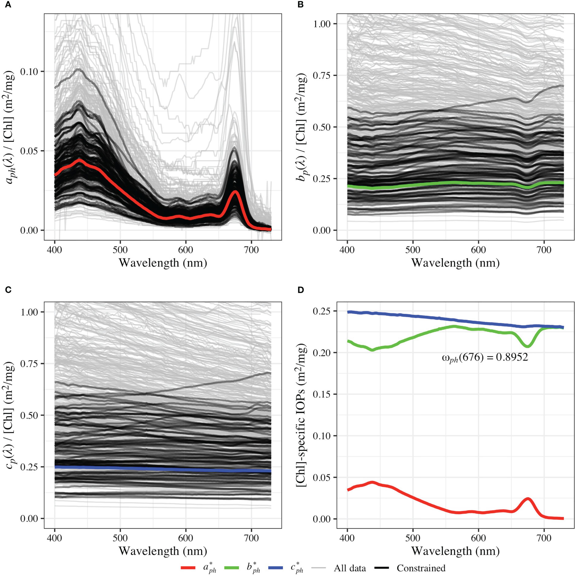
Figure 4 The spectra of Chl-specific IOPs of the “Brown” group, derived from a subset of the Hereon data. Panels (A–C) present the phytoplankton IOP spectra, normalized by [Chl], for absorption, scattering, and attenuation, respectively. The thick black spectra correspond to constrained samples used to determine IOPs. Panel (D) shows the calculated Chl-specific IOPs.

FIGURE 5

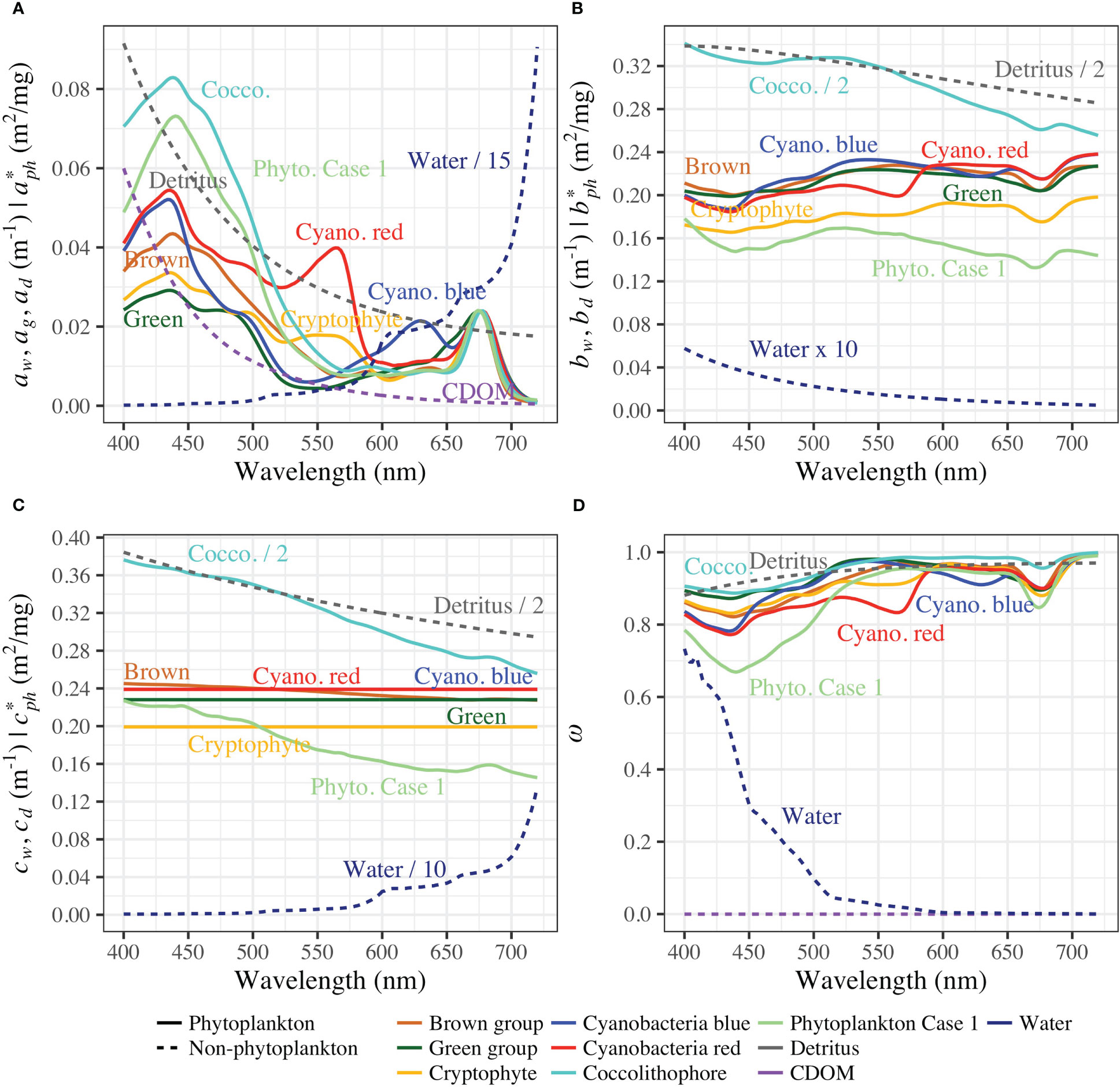
Figure 5 Specific IOPs of phytoplankton groups compared with IOPs of other components. Spectral absorption (A), scattering (B), attenuation (C), and single-scattering albedo coefficients (D) of phytoplankton groups (solid lines) and exemplary non-phytoplankton components (dashed lines): water (with temperature = 20°C and salinity = 15 PSU), detritus (with [ISM] = 1 g/m³ and [Chl] = 3 mg/m³), and CDOM (with a_g (440) = 0.03 m^-1). Some spectra are re-scaled for better visualization.

The backscattering probabilities of phytoplankton, ${\tilde{b}}_{bph}$, is assumed to be spectrally independent (Twardowski et al., 2001; Harmel et al., 2021). Based on the data reported by previous studies (Bricaud et al., 1983; Ahn et al., 1992; Gregg and Rousseaux, 2017), ${\tilde{b}}_{bph}$ of each group are assigned as 0.002 for the “Brown” group and the Cryptophytes, 0.003 for the two Cyanobacteria groups, 0.007 for the “Green” group, the Coccolithophores, and the “Phytoplankton Case-1” group. ${\tilde{b}}_{bph}$ is then calculated as the sum of all group fractions.

To simplify the phytoplankton IOP for oligotrophic Case-1 water, which is typically dominated by Synechococcus sp. and Prochlorococcus sp., we applied constraints to the occurrence of the different groups in the “Two-term” model but not in the “Four-term” model. The distribution of phytoplankton groups was estimated based on open access High Performance Liquid Chromatography (HPLC) data (Kramer and Siegel, 2021) and the CHEMTAX method (Mackey et al., 1996), using the results as a reference. The initial and final pigment ratio matrices can be found in Tables A1, A2 of the Supplementary Material. To account for natural variability in phytoplankton absorption and scattering, we performed random sampling and shuffling to obtain the fractions of the phytoplankton groups, $f_{ph}$, within the upper and lower limits. The fraction library for sampling is presented in Figure A1 of the Supplementary Material. Details of the calculation steps for the “Four-term” and “Two-term” IOP models can be found in Table 3; and a flow chart summarizing the process is provided in Supplemental Figure A2. The relevant data and codes for the IOP model are provided in the section Data Availability Statement.

TABLE 3

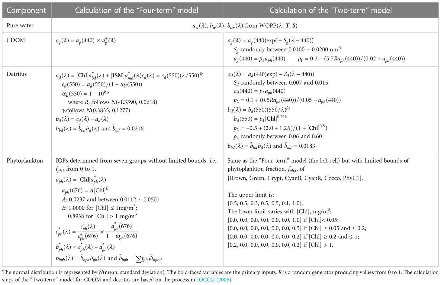
Table 3 Calculation steps of the “Four-term” and “Two-term” IOP models.

3.3 Benchmark tests

3.3.1 Other IOP models

In this study, we compared our proposed IOP model with two other models, R18 (Ramírez-Pérez et al., 2018) and L23M (Loisel et al., 2023). We didn’t consider models designed for retrieving IOPs from AOPs, as our focus is on forward modeling. It should be noted that the performance of a model depends on its inputs and the type of water it is applied to. A superior model should be able to capture the majority of IOPs across various optical water types and accurately reproduce IOPs when component concentrations are provided.

The R18 model estimates specific IOP coefficients of water components using a deconvolution method, based on data from optically complex waters in the Ligurian Sea. Its outputs are deterministic and depend solely on the input variables [Chl], [TSM], and $a_g(440)$.

The L23M model (the “M” indicating it’s a model, as opposed to the name of their data set) was developed as part of the study by Loisel et al. (2023) to create the L23 data set (refer to Table 2). The L23M model is not deterministic, meaning that it does not always produce the same result given the same inputs. This is because the model incorporates random values, which are used to account for natural variability. Its non-deterministic result may fluctuate with changes in random values. To address this, we repeated model runs 30 times for a given input, and calculated the mean and standard deviation for comparison purposes. The same procedure was also implemented for our model.

3.3.2 Remote-sensing reflectance model and simulations

In this study, we adopted the formula proposed by Lee et al. (2011) to simulate $R_{rs}(\lambda )$ based on the absorption and backscattering coefficients obtained from IOP models. The formula is given as:

$\begin{array}{ll}{R}_{rs}(\lambda )=\left(G_0^w+G_1^w\frac{b_{bw}(\lambda )}{k(\lambda )}\right)\frac{b_{bw}(\lambda )}{k(\lambda )}+\left(G_0^p+G_1^p\frac{b_{bp}(\lambda )}{k(\lambda )}\right)\frac{b_{bp}(\lambda )}{k(\lambda )},& (22)\end{array}$

where $k(\lambda )=a_t(\lambda )+b_{bt}(\lambda )$. The coefficients G are dependent on solar zenith angle and viewing direction, with values for solar zenith angle = 30° and nadir viewing direction being $G_0^w$ = 0.05881474, $G_1^w$ = 0.05062697, $G_0^p$ = 0.03997009, and $G_1^p$ = 0.1398902.

To demonstrate the potential of our IOP models in building a synthetic database, we generated a wide range of component concentrations and fed them into Eq. (22). Note that these simulations are a simplified showcase and a full radiative transfer model, such as HydroLight, will be utilized in the future. The range of concentrations was collected from the data sets listed in Table 2. We calculated their mean and standard deviation values and assumed a log₁₀-normal distribution with twice the standard deviation to obtain more samples at extremely low and high values (Campbell, 1995). The concentration specifications are presented in Table 4. We generated 1,000 random combinations and to capture more variability in Case-2 waters, we used these combinations eight and four times in “Four-term” and “Two-term” models, respectively, resulting in 12,000 simulations.

TABLE 4

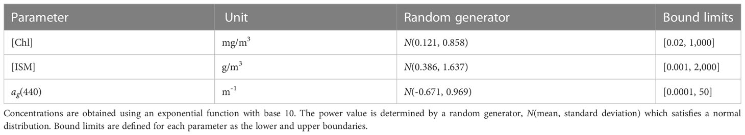
Table 4 The specifications of component concentrations in the IOP simulation.

3.3.3 Alternative phytoplankton scattering assumption

Many contemporary inversion models, used for deriving IOPs from AOPs, commonly employ power law functions to represent particle scattering or backscattering (Lee et al., 2002; Maritorena et al., 2002; Morel et al., 2002; Werdell et al., 2013; Liu et al., 2020). Although this parameterization has been successful in retrieving IOPs for decades, there is less confidence in the accuracy of scattering coefficients (Roesler and Boss, 2003) due to the non-smooth nature of the scattering spectra, as observed from in situ measurements and theoretical models (Babin et al., 2003a; Stavn and Richter, 2008; Bernard et al., 2009). In contrast, particulate attenuation spectra, such as those in the Hereon data set shown in Figure 4, exhibit more smoothness, whereas scattering spectra tend to be more irregular in the wavelength range where absorption spectra display peaks. This is believed to result from the compensation of strong absorption peaks by phytoplankton (Twardowski et al., 2001). This raises the question of how the use of a smoothed power law function for scattering spectra in the presence of spectral features affects the accuracy of the ocean color algorithm.

In this study, we used the Gordon and Morel (1983) model, which is a common option in HydroLight, to examine the impact of the $b_{ph}$ assumption on $R_{rs}$ simulation. The power law model is expressed as:

$\begin{array}{ll}{b}_{ph}^{\text{GM}83}(\lambda )=b_0{[\text{Chl}]}^n{\left(\frac{{\lambda }_0}{\lambda }\right)}^m,& (23)\end{array}$

where $b_{ph}^{\text{GM}83}(\lambda )$ represents the $b_{ph}(\lambda )$ by the above model, ${\lambda }_0$ = 550 nm, $b_0$ = 0.3, $n$ = 0.62, and $m$ = 1. The term $b_0{[\text{Chl}]}^n$ denotes that $b_{ph}(550)$ is dependent on [Chl], and the spectral shape is controlled by the exponent $m$. The observed difference in magnitude may be due to the varying relationship between $b_{ph}(550)$ and [Chl] across different aquatic systems. To account for this magnitude effect, we adjusted $b_{ph}^{\text{GM}83}(\lambda )$ by normalizing its $b_{ph}^{\text{GM}83}(550)$ to the value obtained from our IOP model. This leads to $b_{ph}^{\text{Adj}}(\lambda )$, which is calculated as:

$\begin{array}{ll}{b}_{ph}^{\text{Adj}}(\lambda )=b_{ph}^{\text{GM}83}(\lambda )\frac{b_{ph}(550)}{b_{ph}^{\text{GM}83}(550)},& (24)\end{array}$

where $b_{ph}(\lambda )$ , for the sake of simplification, is the phytoplankton scattering coefficients by our IOP model. We conducted a sensitivity analysis to compare the simulated $R_{rs}$ using $b_{ph}$, which is assumed as the reference, and the two modified scattering assumptions $b_{ph}^{\text{GM}83}$ and $b_{ph}^{\text{Adj}}$.

3.4 Statistical metrics for evaluating model performance

This study evaluated the performance of an IOP model by comparing its ability to reproduce co-measured concentrations and IOP results using component concentrations as input. The aim was to demonstrate the capability to accurately describe the bio-optical process. To evaluate the performance, several statistical metrics including linear regression were utilized. The squared correlation coefficient, R², measures how well a model fits the observed data. The slope, S, represents the change in the measured value for each unit increase in the estimated values, while the intercept, I, represents the systematic offset when comparing measurements and estimations. Better fits are indicated by R² and S values closer to one and I value closer to zero. Additionally, the unbiased median percentage difference, D, was used to evaluate the accuracy of IOP models, with lower values indicating better accuracy. D was calculated as the median of $(X-Y)/(X+Y)\times 200\%$ , where X and Y are measurement and estimation values. The measurement and estimation values are scaled using a logarithmic base 10 transformation prior to the calculation of these statistical metrics.

4 Results and discussion

4.1 Reproducibility of IOP models

Recall that the two-term model takes only [Chl] as input, while the four-term model takes [Chl], [ISM], and $a_g(440)$ as inputs. The R18 model uses [Chl], [TSM], and $a_g(440)$, while the L23M model takes only $a_{ph}(\lambda )$. All of these models output spectral IOPs of the components. In this section, we compared these benchmark models in terms of $a_{ph}$, $a_d$, $a_g$, $a_{gp}$, $b_p$, and $b_{bp}$, focusing specifically on the results at 440 nm. Scatter plots for the Hereon data set and the external data sets are in Figures 6, 7, respectively. Additional scatter plots at other wavelengths are provided in the Supplementary Material (Figures A3, A4: 560 and 670 nm). Figure 8 shows spectral analysis to evaluate model performance from 400 to 700 nm. Multispectral samples were excluded in the spectral analysis to avoid outliers, primarily from OC-CCI v3, resulting in different valid estimation numbers (N) in scatter plots and spectra plots, but this does not significantly affect the spectral trend.

FIGURE 6

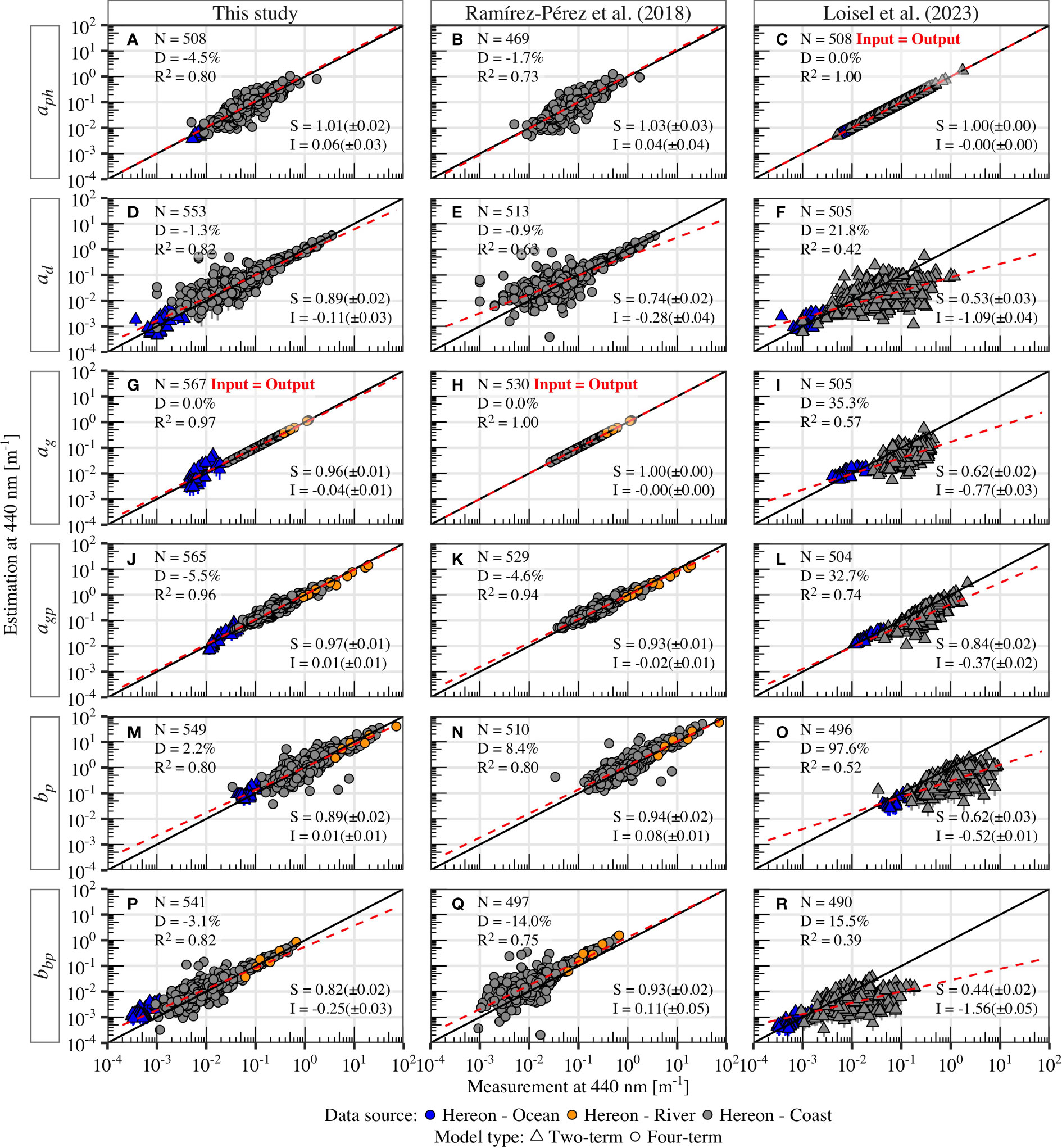
Figure 6 Evaluation of IOP estimates at 440 nm from our proposed model, from Ramírez-Pérez et al. (2018), and Loisel et al. (2023). Color shows the different parts in the Hereon data, shape indicates the model type, black line is 1:1, red line is linear regression. Point denotes the mean value of repeated runs and error bar shows the variation using random parameters (defined in Table 3). Statistics: the number of points (N), the unbiased median percentage difference (D), the coefficient of determination (R²), and linear regression slope and intercept (S and I), with standard deviation in brackets. Panels with notes in red text mean input equals to output. The reason for the absence of results for Hereon – Ocean in R18 is the unavailability of the input parameter [TSM] in that specific part of the data. The panels are labeled from (A–R) corresponding to the different models across the variables.

FIGURE 7

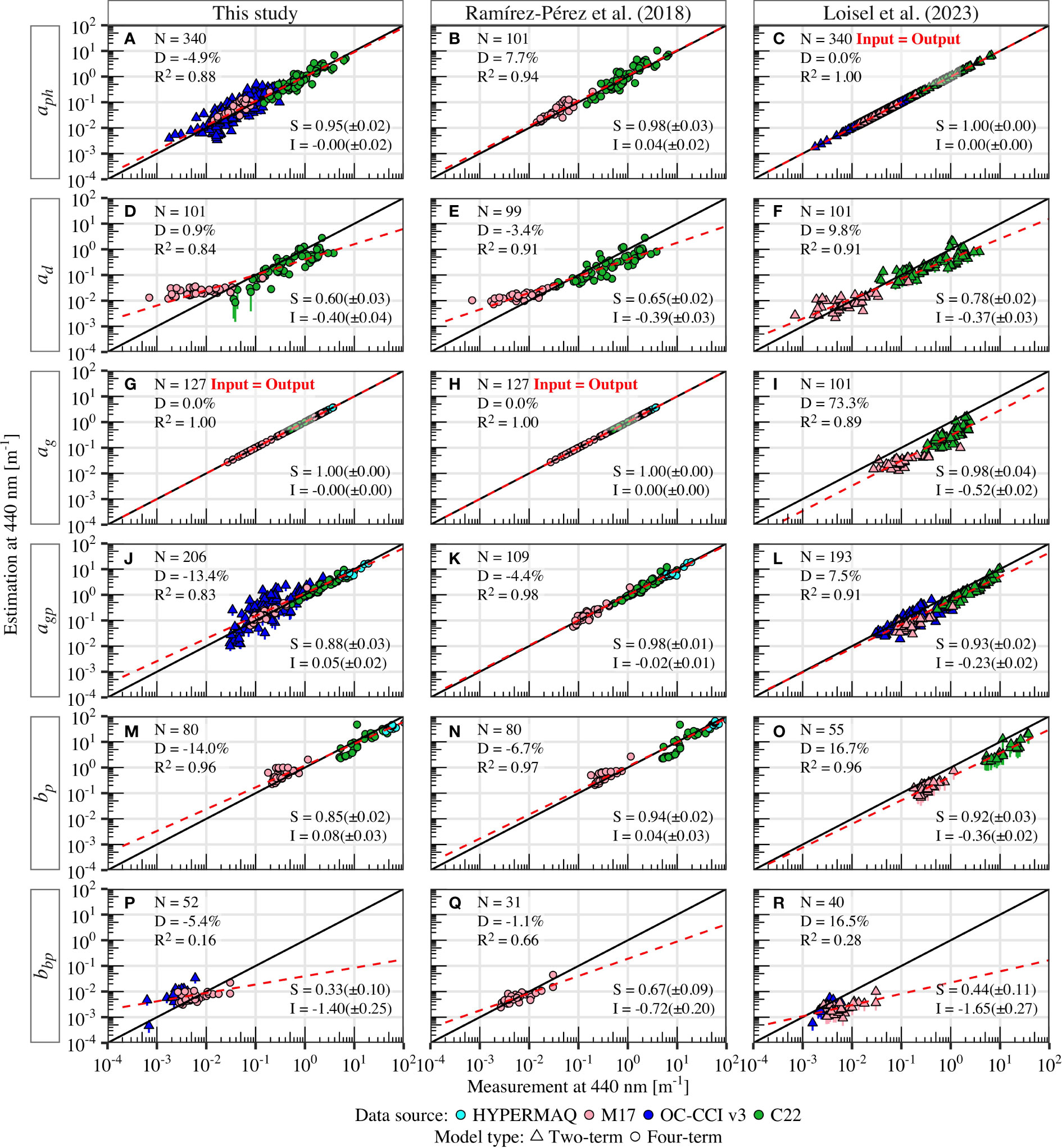
Figure 7 Same as Figure 6 but for external data sets: HYPERMAQ, M17, OC-CCI v3, and C22, shown in different colors.

FIGURE 8

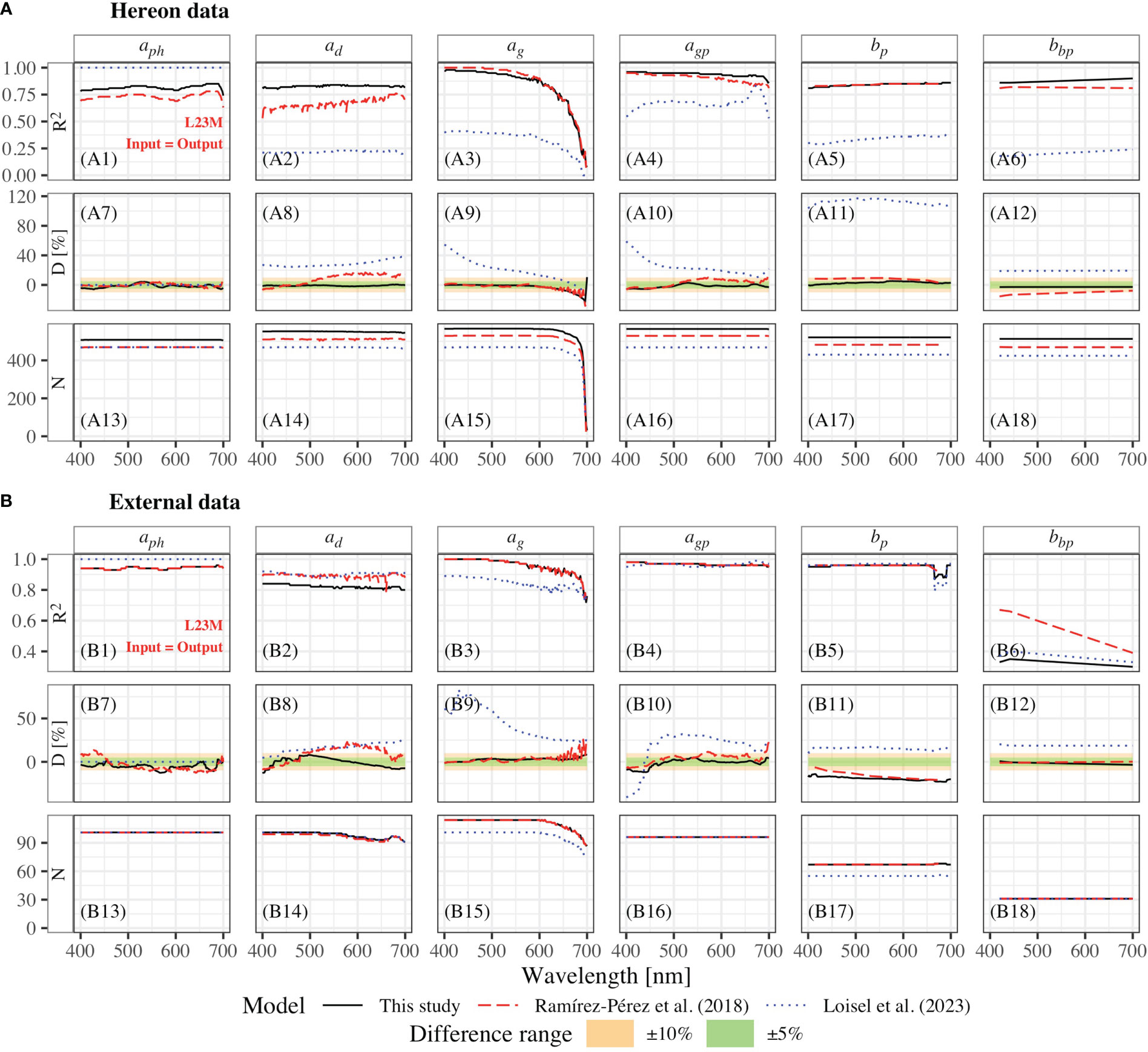
Figure 8 Statistical metric spectral distribution for component IOPs: R², percentage difference (D), and number of valid estimations (N). The lines represent our proposed model, Ramírez-Pérez et al. (2018), and Loisel et al. (2023). Panel (A) uses the Hereon data, while panel (B) uses external data sets listed in Table 2. The wavelength range is from 400 to 700 nm. The two colored shadows represent the percentage differences of ±5% and ±10%, respectively. The model inputs equal to the model outputs for a_ph in the Loisel et al. (2023) model. Some spectra overlap due to the closely similar values.

Figure 6 shows the reproduced IOPs for the Hereon data from our model in comparison with two other models, whereby for our model, the “Two-term” setup was applied to the oceanic data in Hereon and the “Four-term” setup to coastal and river data. The comparison between the two- and four-term results of the “oceanic” samples indicates no significant deviation, which is crucial for the seamless modeling of IOPs during the transition from Case-1 to Case-2 waters. Figure 6A demonstrated accurate $a_{ph}(440)$ estimates with a slope close to one, which verifies the reliability of the $a_{ph}^{*}(\lambda )$ determination and the phytoplankton group spectral shapes, as the result at 440 nm can be regarded as being extrapolated from 676 nm. The percentage difference in $a_{ph}$ from 400 to 700 nm, shown in Figure 8 (A7), was within approximately ±5%, with some results within ±10%. The evaluation of $a_d(440)$ in Figure 6D revealed good performance across a range of four orders of magnitude, especially when $a_d(440)$ was greater than 0.1 m^-1, where the particulate matter was dominated by the inorganic component. However, the $a_d(440)$ estimation was more scattered for lower values, possibly due to increased variability in the $a_{bd}^{*}(\lambda )$ shape due to increased organic components and uncertainties in concentration inputs caused by general measurement errors for organically dominated [TSM], hence [ISM]. The spectral statistical results of $a_d$ in Figure 8 (A8) exhibited relatively consistent values across the wavelength range, with percentage differences between ±5%. The $a_g(440)$ results, shown in Figure 6G, were in line with the “Four-term” input, while the “Two-term” results were dependent on the random parameter values. Despite the wide variation range, the error lines covered the measured values. The statistical results of $a_g$ in Figure 8 (A9) showed percentage differences within ±5% up to 600 nm, but degradation was observed beyond 600 nm as the values approached zero. Our IOP model performed well in the evaluation of $a_{gp}(440)$, the sum of $a_{ph}(440)$, $a_d(440)$, and $a_g(440)$, across different water types and over wavelengths, with no outliers observed. The $b_p(440)$ estimates, shown in Figure 6M, were accurate across three orders of magnitude, but with a few outliers due to higher measurement variation of [TSM]. The $b_{bp}(440)$ results were close to the 1-to-1 line for values greater than 0.01 m^-1, but with some deviations in the low-value region, especially for the “Two-term” model in the oceanic data. The spectral distribution of statistical values for $b_p$ and $b_{bp}$ in Figure 8A remained consistent, with percentage differences within ±5%.

The R18 model generally yielded comparable results at 440 nm to our model, albeit with some differences for certain parameters. Specifically, R18 model underestimated $a_d$ at longer wavelengths, as shown in Figure 8 (A8), with a slope of 0.78 lower than that of our model (0.93) at 560 nm, and with 0.71 lower than 0.99 at 670 nm. This difference could be due to the imperfect separation of biogenic and minerogenic parts of detritus in R18, as the pigment residuals in longer wavelengths, e.g., ≥ 560 nm, were still evident in their $a_{bd}^{*}(\lambda )$ , leading to the underestimation of $a_{md}^{*}(\lambda )$ in these wavelengths. Additionally, consistent discrepancies between measurements and estimations of $b_p(\lambda )$ and $b_{bp}(\lambda )$ were observed across wavelengths, which were also found in other data sets, as shown in Figure 8B. Based on the points of Hereon – Ocean and some points of Hereon – Coast resembling oceanic waters, as shown in Figure 6, the L23M model demonstrates favorable results for Case-1 waters when $a_{ph}(\lambda )$ spectra are provided. Conversely, the model generally underestimates all IOPs for Case-2 waters across the wavelength range concerned, as demonstrated in Figure 8B. This outcome is anticipated since the model is primarily designed for global oceanic waters. The superior performance of the L23M model for Hereon – Ocean is primarily due to the fact that $a_{ph}(\lambda )$ is its primary input, which mainly governs the total IOPs.

Figure 7 displays an independent evaluation of IOP models based on in situ data from external sources. Our model performs better in estimating $a_{ph}(440)$ for various water types, including CDOM-dominated lakes from M17, eutrophic lakes from C22, and oceanic waters from OC-CCI v3, as evidenced by the lower percentage difference. In addition, our model produces a larger number of estimated $a_{ph}(440)$ values, which may interfere with the reliability of other statistical metrics if other models are unable to estimate these points. However, the $a_d(440)$ results are slightly underestimated in C22 and overestimated M17 in both our model and R18. The higher [ISM] values observed in M17 compared to similar samples in the Hereon data may explain the overestimation of $a_d(440)$, which can also be observed from the overestimation of $b_p(\lambda )$ in Figures 7M, N. The overestimation of $a_d(\lambda )$ was slightly reduced by L23M in Figure 7F, when only [Chl] was used to model $a_d(\lambda )$. One should consider the uncertainty associated with component concentration when using IOP models (IOCCG, 2019). Despite this, the overall performance of $a_{gp}(440)$ remains strong by our model, with an R² of 0.83, even in the presence of more variability in OC-CCI v3. The spectral percentage difference of $a_{gp}$ mostly fell within ±10%, as shown in Figure 8 (B10). The $b_p(440)$ estimates by our model are slightly underestimated for extremely turbid water (mainly from HYPERMAQ). For such highly turbid waters, the uncertainty of in situ measurements should be considered (IOCCG, 2019). Only a few of points of $b_{bp}(\lambda )$ are observed due to the limited data from these external data sets. The different performance between our model and R18 in estimating $b_{bp}(440)$ may result from the use of similar measurement devices in the studies of R18 and M17. The reason for the absence of results for Hereon – Ocean and OC-CCI v3 in R18 is the unavailability of the input parameter [TSM] in that specific part of the data. Note that the smaller data size and larger measurement uncertainties in the external data sets compared to the Hereon data can impact statistical results in Figure 8B. Nonetheless, our model still demonstrates consistent and robust performance across the spectrum, with most components falling within a ±10% difference range.

To summarize, our IOP model shows comparable performance as other the two models in terms of reproducing IOPs from concentrations in specific water environments and in terms of absolute values and spectral shapes. However, our model provides a higher amount of reproducibility across diverse optical water types, encompassing oceanic, coastal, and inland waters. Our spectral statistical metrics demonstrate that the estimations of model have a percentage difference of within ±5% for most component IOPs throughout the visible spectrum, with some falling within ±10%, which is essential for meeting the accuracy requirements outline in GCOS (2011) for developing ocean color algorithms. Another advantage of our IOP model is its flexibility, allowing for replacement of specific model parameters with more optimal values in special scenarios. Although these parameters defined so far have proven to be representative, this enables continuous improvement and refinement of the model over time.

4.2 Do we capture most optical variability?

In the previous section, we established that our IOP model can accurately reproduces water optical properties based on component concentrations. However, we also need to determine whether the model can capture most of the optical variability, which depends on the concentration range and the dynamic range of model parameters like $\gamma$ and $\omega$. We admit that our current ranges may not encompass some extreme scenarios. For instance, to address the underestimation depicted in Figure 7M, we increased the original value of ${\omega }_d(550)$ and reduced ${\gamma }_d$ to simulate a highly turbid water type. By adjusting model parameters such as $\gamma$ and $\omega$, the resulting ranges offer valuable insights into the appropriate direction for fine-tuning the model. Although these modifications improved that particular case, they lay outside 96% of the training data distribution. Despite this, we used the original model parameters established in section 3.2 and the concentration range provided in Table 4 to do the simulation as a showcase, which is used to test the data coverage with other data sets.

The data distribution presented in Figure 9 compares in situ measurements and simulated data sets. Panels (A) and (C) show our simulated data and in situ measurements, while panels (B) and (D) compare other simulated data sets. Our selection of 560 nm was intended to showcase the data distribution, but it is worth noting that the results for other wavelengths are also comparable. The $a_p(560)$ and ${\omega }_p(560)$ relationships demonstrate the ratio of $b_p$ to $c_p$ as particle absorption increases. The $a_p(560)$ values of Hereon vary up to four orders of magnitude, with C22 and HYPERMAQ having higher values, and M17 varying over a smaller range with lower values. Despite the variation in $a_p(560)$, Figure 9A demonstrates that the variation in ${\omega }_p(560)$ is relatively stable, with measured values as low as about 0.9 and simulated values as low as 0.8. As anticipated, the “Four-term” model contributes to most of the value variation. Figure 9B indicates that other simulated data sets have similarities, with the L23 data set having a comparable distribution to our simulations, albeit with fewer points where $a_p(560)$ is greater than 0.1. The simulated CCRR data set shows a wider distribution in $a_p(560)$ but stable ${\omega }_p(560)$, primarily due to a constant ${\gamma }_d$ and a [Chl]-related ${\gamma }_{ph}$. However, the simulated C2X data set displays more pronounced differences, with some points having significantly lower ${\omega }_p(560)$ values for high $a_p(560)$ and phytoplankton-dominated water, suggesting that only 20% of the light is scattered for a given high particle concentration, resulting in low reflectance, which is inconsistent with real-world observations. The primary reason for such low ${\omega }_p(560)$ values is the inappropriate parameterization of $b_{ph}(\lambda )$ in C2X. These points have lower $b_{ph}(\lambda )$ values with relatively higher $a_{ph}(\lambda )$ (not shown). Figures 9C, D show the relationship between $a_{gp}(560)$ and $b_{bp}(560)$, with $b_{bp}(560)$ increasing as $a_{gp}(560)$ increases in the measured data, suggesting a stable proportion of $a_g(560)$ in $a_{gp}(560)$ that co-varies with [Chl], as reflected in CCRR and L23. C2X contains simulations of extremely absorbing waters, resulting in simulated points below the distribution of other data due to high CDOM absorption. Our simulated data, using a similar concentration limit from C2X, has a wider coverage compared to the C2X distribution, with most points originating from the “Four-term” model (CDOM is independent of [Chl]), while C2X has some data gaps.

FIGURE 9

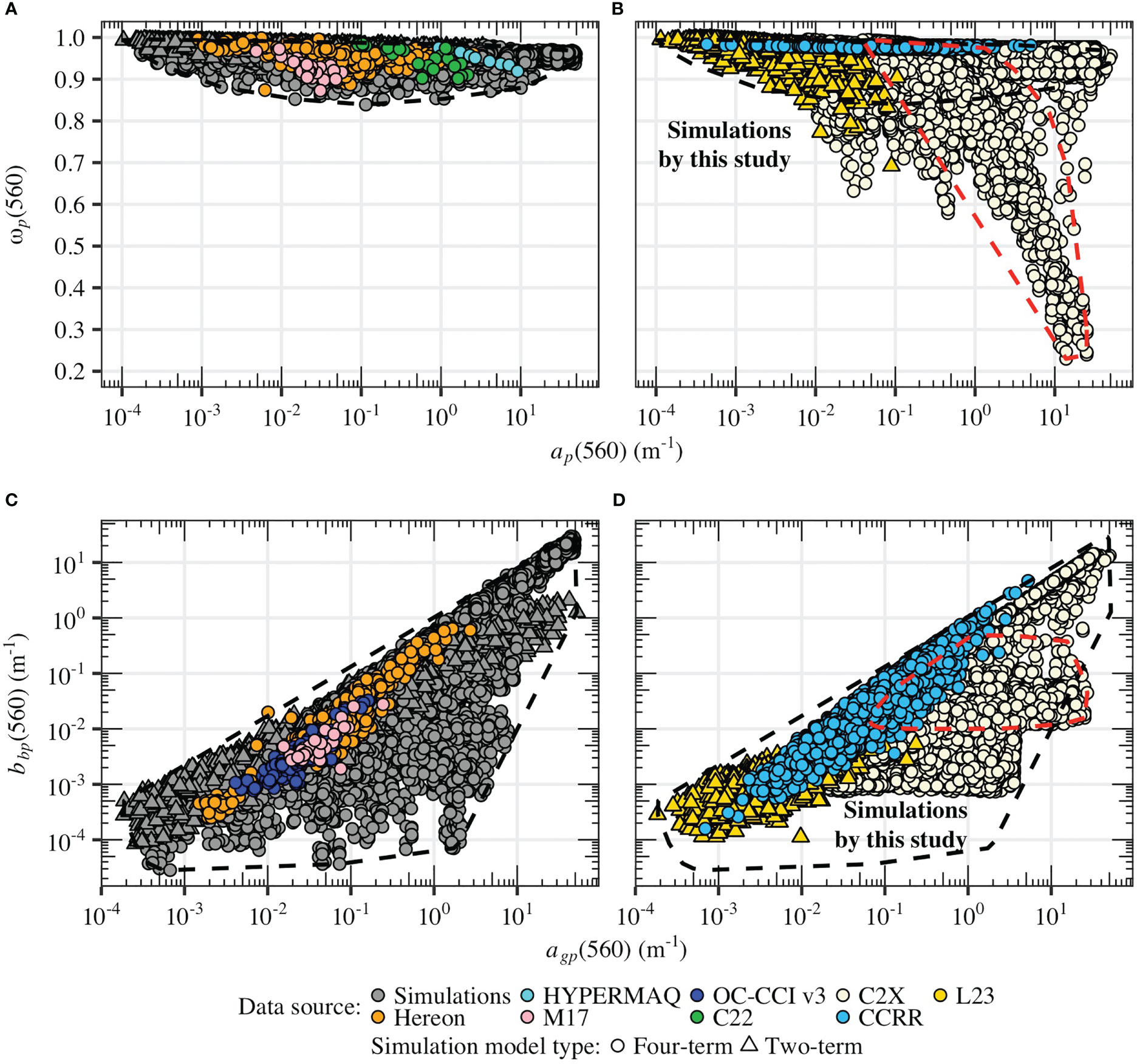
Figure 9 Data coverage comparison for IOPs at 560 nm of our simulated data with measured (left) and other simulated (right) data. (A, B) show scatter plots of particulate absorption versus the single-scattering albedo. (C, D) show the total non-water absorption versus total particulate backscattering. The black dashed outline is the convex hull of our simulations and the red one is highlighted part in the C2X data set that [Chl] ≥ 50 mg/m³ and [ISM] ≤ 50 g/m³.

For practical reasons, the study limited the number of IOP components to a manageable amount instead of including all particle species in water (Stramski et al., 2004). In the “Four-term” model, $a_g$ was modeled using a few spectra (N=12) with similar shapes ($S_g$ = 0.0174 nm^-1 ± 0.1%). The resulting model was able to accurately reproduce the CDOM spectrum with precise $a_g(440)$ values. In the “Two-term” model, $a_g$ was correlated to [Chl] with a random value, resulting in relatively greater variability, but still covering the range of values observed in oceanic waters. The shape of specific detritus absorption, $a_d^{*}$, varies across different aquatic environments but is generally limited on a local scale (Woźniak and Dera, 2007). The slope of minerogenic detritus absorption, $S_{md}^{*}$, in our study, 0.0104 nm^-1 in Figure 2B, was consistent with values observed in other natural water basins (Woźniak and Dera, 2007). The combination of biogenic and minerogenic detritus in our model enhances its applicability across different regions, which is important for simulating IOPs of complex waters on a global scale. The use of different quantiles (quasi-organic proportion of the total particle) to define $a_{bd}^{*}$ aligns with the observed increase in biogenic detritus absorption when organic matter dominates. The slopes of our simulated $a_d$ values range from 0.0068 to 0.015 (as per the definition in Stramski et al. (2019), based on the natural logarithmic transformation at 440 and 550 nm), which are generally consistent with previous studies, e.g., 0.0095~0.0148 in Zheng et al. (2015) and 0.0031~0.0169 in Stramski et al. (2019), but lack the “flat” shapes (lower values) found in Stramski et al. (2019) due to limited data in the training set, which can be expanded in the future to incorporate such extreme scenarios. The IOP model proposed in this study includes seven phytoplankton groups that are used as general “color” groups, rather than specific phytoplankton species or functional types that have different absorption and scattering properties. By using these general groups, the model can capture the increased variability in phytoplankton IOPs that is visually seen in natural systems. In other words, the phytoplankton groups in our model are not based on specific biological characteristics, but rather on their broad spectral characteristics, allowing for more flexibility and accuracy in predicting phytoplankton IOPs. Variables $a_{ph}(412)/a_{ph}(443)$ and $a_{ph}(555)/a_{ph}(490)$, used to describe the shape of $a_{ph}$ in Zheng et al. (2015), were found to be in good agreement with other in situ and simulated data sets, within the ranges of 0.8~1.0 and 0.2~1.0, respectively. Although some ranges may not be covered, it is not necessary to add more phytoplankton groups if no color differences are added. Our IOP model is also able to simulate coccolithophore blooms with a 490 nm reflectance peak by multiplying its absorption coefficient by 0.02, which is biologically based on the vanishing of the absorbing algae cells but remaining high scattering from detached coccoliths (Neukermans and Fournier, 2018; Cazzaniga et al., 2021).

Complete coverage of the optical diversity of as many natural waters as possible is also important for the exploitation of optical water type classification methods. Existing methods (e.g., Moore et al., 2014; Hieronymi et al., 2017; Jackson et al., 2017; Bi et al., 2021) can only partially cover the optical variability; many complex waters are out-of-scope for these methods, which is reflected in too low class memberships (not shown in detail here). This also applies to the classifiability of $R_{rs}$ from various ocean color atmospheric corrections (Hieronymi et al., 2023). Both aspects identify potential weaknesses of the OWT methods, which should be revised in the future, e.g., by means of our IOP model. It is noteworthy that the analysis here did not account for variability when modeling IOP to $R_{rs}$, and we simplified backscattering as a spectral constant rather than a sophisticated phase function or a volume scattering function. This could impact the $R_{rs}$ angular distribution in many complex waters (Harmel et al., 2016). When analyzing OWT frameworks, environmental factors, and sun-viewing geometries should also be considered and varied (Bi et al., 2023).

4.3 Sensitivity analysis of phytoplankton scattering assumption

Figure 10 demonstrates that the disparity in $R_{rs}$ between modeled $b_{ph}(\lambda )$ and $b_{ph}^{\text{GM}83}(\lambda )$ was more noticeable at high [Chl] (>100 mg/m³), with $b_{ph}^{\text{GM}83}(\lambda )$ showing lower values (up to 0.02 sr^-1 difference) due to the modeled $b_{ph}(550)$ discrepancy. At low [Chl] (< 1 mg/m³), $b_{ph}^{\text{GM}83}(\lambda )$ displayed slightly higher $R_{rs}$ values (up to 0.003 sr^-1 or 40% difference). The most significant differences were observed in the green and NIR (540~590 nm and 700~730 nm), with differences of up to 90%, while the blue region (400~450 nm) was the least affected as non-phytoplankton signals prevail. Renormalizing $b_{ph}^{\text{GM}83}(\lambda )$ to $b_{ph}^{\text{Adj}}(\lambda )$, which makes $b_{ph}^{\text{Adj}}(560)$ equal to $b_{ph}(560)$, significantly reduced differences in $R_{rs}$ except for higher [Chl] (>100 mg/m³). However, the values in NIR were still lower than those with $b_{ph}(\lambda )$ by up to 0.004 sr^-1 (or 35%). Figure 11 presents six intuitive samples of IOPs and $R_{rs}$ ordering by increasing [Chl] values. The use of $b_{ph}^{\text{GM}83}(\lambda )$ underestimated $b_p(\lambda )$ from concentrations evaluated in the training and testing data sets (not shown) and did not fit the spectral features of phytoplankton observed in the measured $b_p$ data (Castagna et al., 2022; Röttgers et al., 2023), resulting in suppressed $R_{rs}$ values in the green and longer wavelengths for high [Chl]. This contradicts the high NIR reflectance commonly seen during algal blooms (Hieronymi et al., 2017; Bi et al., 2019; Castagna et al., 2022). The differences were significantly mitigated by using $b_{ph}^{\text{Adj}}(\lambda )$, although the shape difference still remains.

FIGURE 10

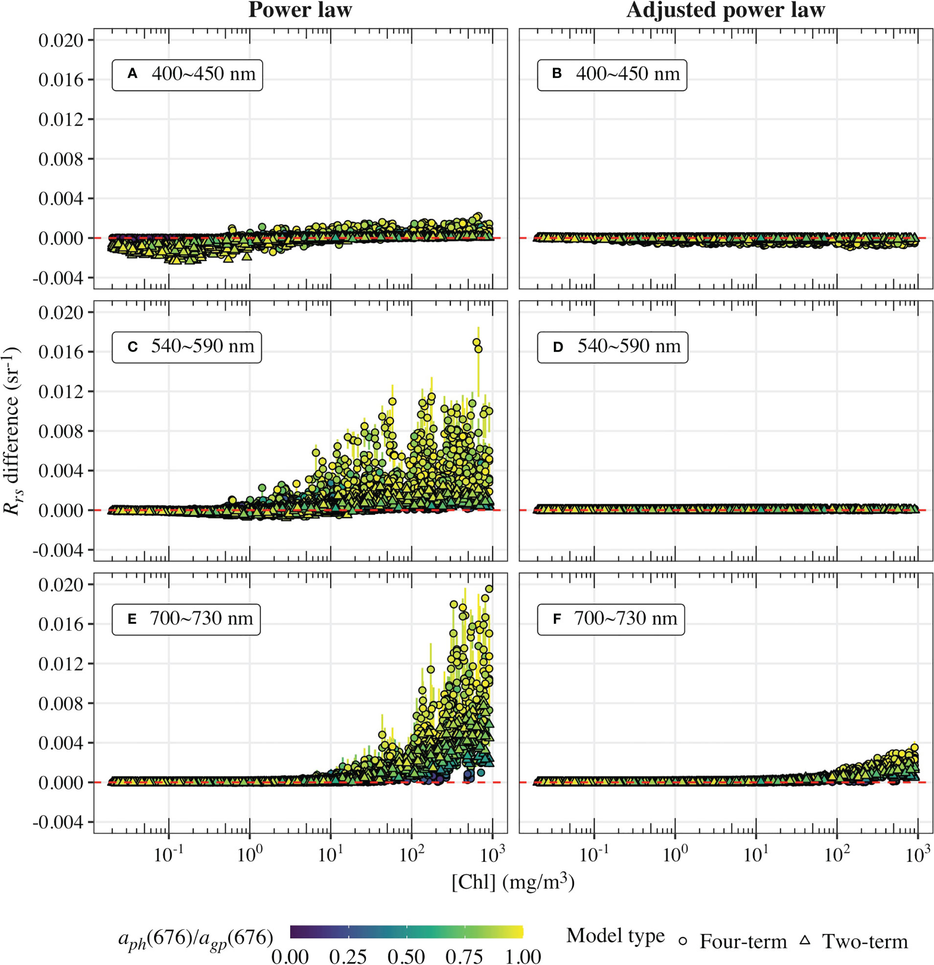
Figure 10 The difference in R_rs due to the scattering assumption of phytoplankton. Points and error bars indicate the mean and range of differences at selected wavelengths. The first column (Power law) represents the results using $b_{ph}^{GM83}(\lambda )$, while the second column (Adjusted power law) $b_{ph}^{Adj}(\lambda )$ (see text). Panels (A, B) for 400~450 nm; (C, D) for 540~590 nm; (E, F) for 700~730 nm.

FIGURE 11

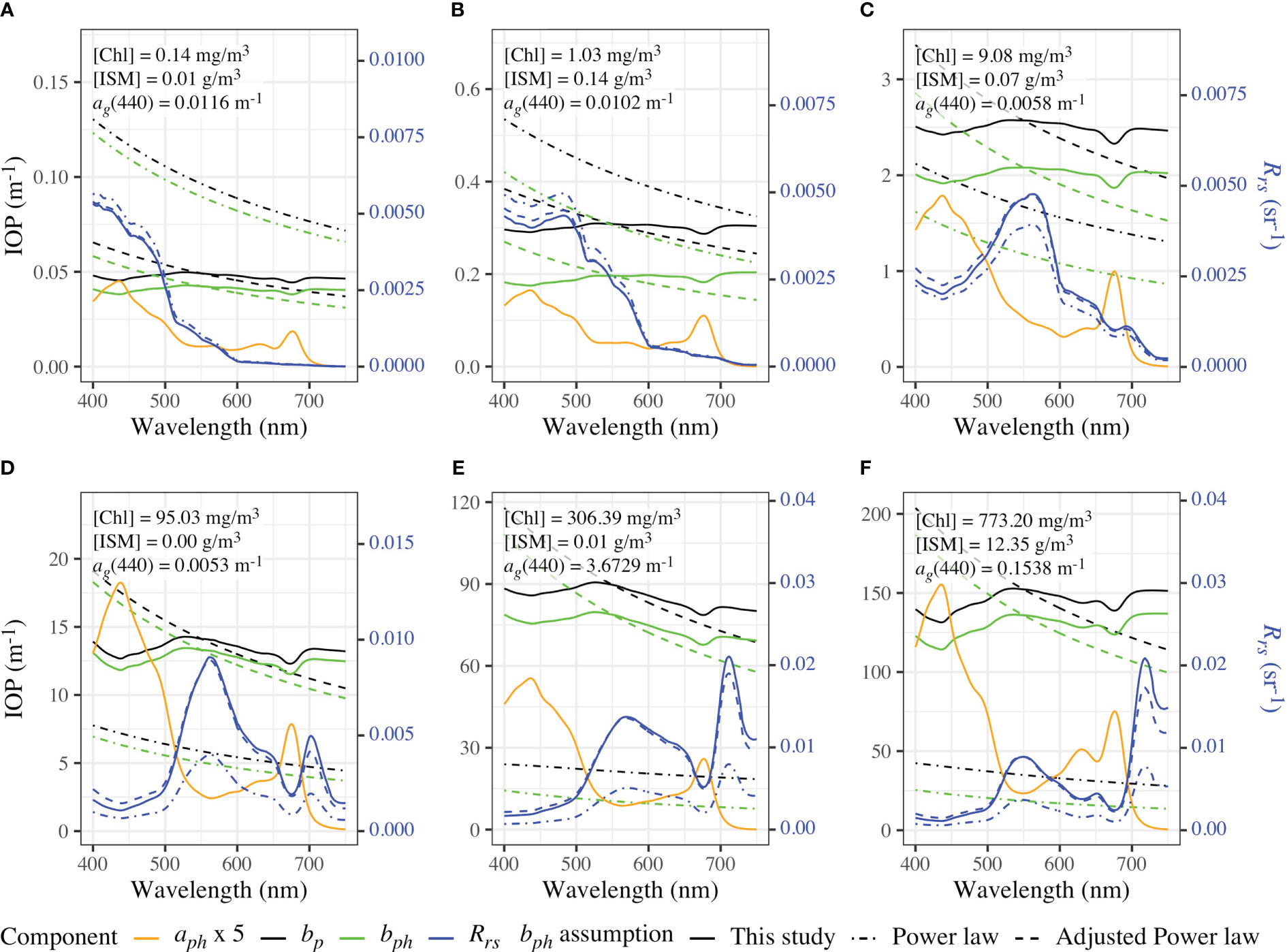
Figure 11 Comparison of the impact of phytoplankton scattering assumptions on IOPs and R_rs in six simulated samples varying from low to high [Chl]. The component concentrations are displayed in the corner of each panel. Panels (A–F) sorted by increasing [Chl].

The sensitivity analysis results, on the forward modeling aspect, revealed that the assumption of $b_{ph}$ shape has a limited impact on $R_{rs}$ modeling, provided that the $b_{ph}$ magnitude is reasonable. This finding may explain why some inversion models perform well, despite using a simplified power law function for scattering shape. However, it is worth noting that the simplified scattering shape may not accurately represent the scattering spectra and may lead to variance transference between scattering and absorption in the non-linear optimizing approach, as discussed in Roesler and Boss (2003) from the perspective of inversion modeling. Furthermore, a power law function may not be sufficient for modeling optically complex water, particularly at high biomass, where scattering dominates over absorption in water color (McLeroy-Etheridge and Roesler, 1998).

It is important to note that adjusting $b_{ph}$ to $b_{ph}^{\text{Adj}}$, as presented in this section, is an ideal scenario that may not always be feasible due to limited knowledge of $b_{ph}$ magnitude in many practical cases. As discussed about the C2X in Figure 9B, modeling absorption and scattering of phytoplankton (detritus as well) separately can lead to significant uncertainties when the input concentrations are outside their training ranges. To address this issue, a relative IOP parameter, the single-scattering albedo, is used in our new model, which has been proven to improve accuracy. Additionally, attenuation, unlike scattering, is relatively simpler to mathematically describe (Twardowski et al., 2001; Roesler and Boss, 2003). Therefore, we suggest an improved parameterization of phytoplankton IOPs in terms of both their spectral shape and magnitude, which has been shown to be applicable for various natural water types.

5 Conclusion

In this study, we introduce a new bio-geo-optical model that can compute spectral inherent optical properties (IOPs) of water constitutes, providing a valuable tool for predicting and understanding the optical properties of natural water. The model presents several advantages including the consideration of the absorption of detritus from biogenic and minerogenic sources, distinctive optical signatures of the phytoplankton communities, and a novel strategy for modeling scattering coefficients that avoids unrealistic simulations observed in previous studies. To parameterize the model, we perform a detailed and comprehensive analysis of high-quality in situ data from optically complex water, and evaluate the model performance using both training and independent data sets. Our model demonstrates promising capabilities in reproducing consistent spectral IOPs from concentrations across different natural water types, including oceanic, coastal, and inland waters. Based on the evaluation both using the training and independent data sets, our model demonstrates an accuracy of within ±5% for most component IOPs throughout the visible spectrum, with some falling within ±10%.

Our new model offers a high degree of freedom, allowing for extensive customization and adaptability when applied to new aquatic systems that extend beyond the training data set. This flexibility enables researchers to fine-tune the framework according to specific requirements, enhancing its practicality and convenience. To fill the gap in previous studies, we generate a showcase data set based on our new model and a simple $R_{rs}$ model, which demonstrates better coverage of the majority of optical variability when compared to several published synthetic data sets. This provides valuable guidance for radiative transfer simulations and building a comprehensive synthetic database for the ocean color community, which should help better distinguish optically active water constituents and thereby reduce uncertainties in ocean color remote sensing. The relevant data and code of the model are available in the section Data Availability Statement.

Data availability statement

The major part of training data set used this study, Hereon, is available on PANGAEA (doi.pangaea.de/10.1594/PANGAEA.950774). The R code for running the model in this study is available in a compiled package, which can be accessed at https://github.com/bishun945/IOPmodel. A web application is also provided to test and run the model at https://bishun945.shinyapps.io/IOPmodel/. Further inquiries can be directed to the corresponding author/s.

Author contributions

The original draft was written by SB under the guidance of RR and MH, who also contributed to the initial paper plan. RR performed the synthesis of the Hereon data set, while MH and RR contributed to the model parameterization. SB synthesized external data sets and implement models included in the manuscript. SB was involved in the development of the model, data processing, and figure production, with input from RR and MH. All authors contributed to the article and approved the submitted version.

Funding

The Helmholtz Association with the research program Earth and Environment (PoF IV) funded this study. Additional support was provided by the Hereon-I²B project PhytoDive. This work builds on fundamental results from the EnMAP scientific preparation program of the DLR Space Administration with funds from the German Federal Ministry for Economic Affairs and Energy, specifically the grants 50EE1718 and 50EE1257.

Acknowledgments

We would like to express our gratitude to the Master and Crew of FS Sonne during SO287 for their valuable assistance and support during the research cruise. We are particularly grateful to Kerstin Heymann and Henning Burmester for their help during the cruise, and to Kerstin Heymann for conducting the chlorophyll measurements. We also extend our appreciation to Dariusz Stramski for generously providing their model data, Simon Wright for providing the CHEMTAX software, Zhongping Lee for providing their model lookup table, and David McKee for providing the model coefficients for the R18 model. We thank Hongyan Xi and Xuerong Sun for the discussion on CHEMTAX. We are also grateful to Daniel Jorge, Bouchra Nechad, André Valente, Colleen Mouw, Héloïse Lavigne, Alexandre Castagna, and their colleagues for providing their data sets, which were vital for our research. We thank the R core team and authors of the R packages for their work in developing and maintaining the free software utilized in this study. We would like to thank the editor Astrid Bracher, and two reviewers for their helpful comments.

Conflict of interest

The authors declare that the research was conducted in the absence of any commercial or financial relationships that could be construed as a potential conflict of interest.

Publisher’s note

All claims expressed in this article are solely those of the authors and do not necessarily represent those of their affiliated organizations, or those of the publisher, the editors and the reviewers. Any product that may be evaluated in this article, or claim that may be made by its manufacturer, is not guaranteed or endorsed by the publisher.

Supplementary material

The Supplementary Material for this article can be found online at: https://www.frontiersin.org/articles/10.3389/fmars.2023.1196352/full#supplementary-material

References

Ahn Y. H., Bricaud A., Morel A. (1992). Light backscattering efficiency and related properties of some phytoplankters. Deep Sea Res. Part Oceanogr. Res. Pap. 39, 1835–1855. doi: 10.1016/0198-0149(92)90002-B

CrossRef Full Text | Google Scholar

Babin M., Morel A., Fournier-Sicre V., Fell F., Stramski D. (2003a). Light scattering properties of marine particles in coastal and open ocean waters asrelated to the particle mass concentration. Limnol. Oceanogr. 48, 843–859. doi: 10.4319/lo.2003.48.2.0843

CrossRef Full Text | Google Scholar

Babin M., Stramski D., Ferrari G. M., Claustre H., Bricaud A., Obolensky G., et al. (2003b). Variations in the light absorption coefficients of phytoplankton, nonalgal particles, and dissolved organic matter in coastal waters around Europe. J. Geophys. Res. 108, 3211. doi: 10.1029/2001JC000882

CrossRef Full Text | Google Scholar

Balch W. M., Holligan P. M., Ackleson S. G., Voss K. J. (1991). Biological and optical properties of mesoscale coccolithophore blooms in the gulf of Maine. Limnol. Oceanogr. 36, 629–643. doi: 10.4319/lo.1991.36.4.0629

CrossRef Full Text | Google Scholar

Balch W. M., Mitchell C. (2023). Remote sensing algorithms for particulate inorganic carbon (PIC) and the global cycle of PIC. Earth-Sci. Rev. 239, 104363. doi: 10.1016/j.earscirev.2023.104363

CrossRef Full Text | Google Scholar

Basedow S. L., McKee D., Lefering I., Gislason A., Daase M., Trudnowska E., et al. (2019). Remote sensing of zooplankton swarms. Sci. Rep. 9, 686. doi: 10.1038/s41598-018-37129-x

PubMed Abstract | CrossRef Full Text | Google Scholar

Bernard S., Probyn T. A., Quirantes A. (2009). Simulating the optical properties of phytoplankton cells using a two-layered spherical geometry. Biogeosci. Discuss 6, 1497–1563. doi: 10.5194/bgd-6-1497-2009

CrossRef Full Text | Google Scholar

Bi S., Li Y., Liu G., Song K., Xu J., Dong X., et al. (2021). Assessment of algorithms for estimating chlorophyll-a concentration in inland waters: a round-robin scoring method based on the optically fuzzy clustering. IEEE Trans. Geosci. Remote Sens. 60, 1–17. doi: 10.1109/TGRS.2021.3058556

CrossRef Full Text | Google Scholar

Bi S., Li Y., Xu J., Liu G., Song K., Mu M., et al. (2019). Optical classification of inland waters based on an improved fuzzy c-means method. Opt. Express 27, 34838–34856. doi: 10.1364/OE.27.034838

PubMed Abstract | CrossRef Full Text | Google Scholar

Bi S., Röttgers R., Hieronymi M. (2023). A transfer model to determine the above-water remote-sensing reflectance from the underwater remote-sensing ratio. Opt. Express. 31, 10512–10524. doi: 10.1364/OE.482395

PubMed Abstract | CrossRef Full Text | Google Scholar

Boss E., Twardowski M. S., Herring S. (2001). Shape of the particulate beam attenuation spectrum and its inversion to obtain the shape of the particulate size distribution. Appl. Opt. 40, 4885. doi: 10.1364/AO.40.004885

PubMed Abstract | CrossRef Full Text | Google Scholar

Bracher A., Bouman H. A., Brewin R. J. W., Bricaud A., Brotas V., Ciotti A. M., et al. (2017). Obtaining phytoplankton diversity from ocean color: a scientific roadmap for future development. Front. Mar. Sci. 4. doi: 10.3389/fmars.2017.00055

CrossRef Full Text | Google Scholar

Brewin R. J. W., Sathyendranath S., Hirata T., Lavender S. J., Barciela R. M., Hardman-Mountford N. J. (2010). A three-component model of phytoplankton size class for the Atlantic ocean. Ecol. Model. 221, 1472–1483. doi: 10.1016/j.ecolmodel.2010.02.014

CrossRef Full Text | Google Scholar

Brewin R. J. W., Sathyendranath S., Kulk G., Rio M.-H., Concha J. A., Bell T. G., et al. (2023). Ocean carbon from space: current status and priorities for the next decade. Earth-Sci. Rev. 240, 104386. doi: 10.1016/j.earscirev.2023.104386

CrossRef Full Text | Google Scholar

Bricaud A., Babin M., Morel A., Claustre H. (1995). Variability in the chlorophyll-specific absorption coefficients of natural phytoplankton: analysis and parameterization. J. Geophys. Res. 100, 13321. doi: 10.1029/95JC00463

CrossRef Full Text | Google Scholar

Bricaud A., Claustre H., Ras J., Oubelkheir K. (2004). Natural variability of phytoplanktonic absorption in oceanic waters: influence of the size structure of algal populations. J. Geophys. Res. 109, C11010. doi: 10.1029/2004JC002419

CrossRef Full Text | Google Scholar

Bricaud A., Morel A., Babin M., Allali K., Claustre H. (1998). Variations of light absorption by suspended particles with chlorophyll a concentration in oceanic (case 1) waters: analysis and implications for bio-optical models. J. Geophys. Res. Oceans 103, 31033–31044. doi: 10.1029/98JC02712

CrossRef Full Text | Google Scholar

Bricaud A., Morel A., Prieur L. (1983). Optical efficiency factors of some phytoplankters1: phytoplankton optical properties. Limnol. Oceanogr. 28, 816–832. doi: 10.4319/lo.1983.28.5.0816

CrossRef Full Text | Google Scholar

Campbell J. W. (1995). The lognormal distribution as a model for bio-optical variability in the sea. J. Geophys. Res. 100, 13237. doi: 10.1029/95JC00458

CrossRef Full Text | Google Scholar

Castagna A., Amadei Martínez L., Bogorad M., Daveloose I., Dassevile R., Dierssen H. M., et al. (2022). Optical and biogeochemical properties of Belgian inland and coastal waters. Earth Syst. Sci. Data. 14, 2697–2719. doi: 10.5194/essd-14-2697-2022

CrossRef Full Text | Google Scholar

Cazzaniga I., Zibordi G., Mélin F. (2021). Spectral variations of the remote sensing reflectance during coccolithophore blooms in the Western black Sea. Remote Sens. Environ. 264, 112607. doi: 10.1016/j.rse.2021.112607

CrossRef Full Text | Google Scholar

Churilova T., Suslin V., Krivenko O., Efimova T., Moiseeva N., Mukhanov V., et al. (2017). Light absorption by phytoplankton in the upper mixed layer of the black Sea: seasonality and parametrization. Front. Mar. Sci. 4. doi: 10.3389/fmars.2017.00090

CrossRef Full Text | Google Scholar

Doerffer R., Schiller H. (2000). “Neural network for retrieval of concentrations of water constituents with the possibility of detecting exceptional out of scope spectra,” in IGARSS 2000. IEEE 2000 International Geoscience and Remote Sensing Symposium. Taking the Pulse of the Planet: The Role of Remote Sensing in Managing the Environment. Proceedings (Cat. No.00CH37120), Honolulu, HI, USA 2,714–717 (IEEE). doi: 10.1109/IGARSS.2000.861680

CrossRef Full Text | Google Scholar

Doerffer R., Schiller H. (2007). The MERIS case 2 water algorithm. Int. J. Remote Sens 28, 517–535. doi: 10.1080/01431160600821127

CrossRef Full Text | Google Scholar

GCOS (2011) Systematic observation requirements for satellite-based products for climate. Available at: https://library.wmo.int/doc_num.php?explnum_id=3710.

Google Scholar

Gordon H. R., Morel A. Y. (1983) Remote assessment of ocean color for interpretation of satellite visible imagery: a review (Accessed January 26, 2022).

Google Scholar

Gregg W. W., Rousseaux C. S. (2017). Simulating PACE global ocean radiances. Front. Mar. Sci. 4. doi: 10.3389/fmars.2017.00060

CrossRef Full Text | Google Scholar

Harmel T., Agagliate J., Hieronymi M., Gernez P. (2021). Two-term reynolds–McCormick phase function parameterization better describes light scattering by microalgae and mineral hydrosols. Opt. Lett. 46, 1860. doi: 10.1364/OL.420344

PubMed Abstract | CrossRef Full Text | Google Scholar

Harmel T., Hieronymi M., Slade W., Röttgers R., Roullier F., Chami M. (2016). Laboratory experiments for inter-comparison of three volume scattering meters to measure angular scattering properties of hydrosols. Opt. Express 24, A234. doi: 10.1364/OE.24.00A234

PubMed Abstract | CrossRef Full Text | Google Scholar

Helms J. R., Stubbins A., Ritchie J. D., Minor E. C., Kieber D. J., Mopper K. (2008). Absorption spectral slopes and slope ratios as indicators of molecular weight, source, and photobleaching of chromophoric dissolved organic matter. Limnol. Oceanogr. 53, 955–969. doi: 10.4319/lo.2008.53.3.0955

CrossRef Full Text | Google Scholar

Hieronymi M., Bi S., Müller D., Schütt D., Behr D., Brockmann C., et al (2023). Ocean color atmospheric correction methods in view of usability for different optical water types. Front. Mar. Sci. 10.

Google Scholar

Hieronymi M., Krasemann H., Müller D., Brockmann C., Ruescas A. B., Stelzer K., et al. (2016). “Ocean colour remote sensing of extreme case-2 waters,” in Proc. Living Planet Symposium, Prague, Czech Republic. 1–5, ESA SP-740.

Google Scholar

Hieronymi M., Müller D., Doerffer R. (2017). The OLCI neural network swarm (ONNS): a bio-Geo-Optical algorithm for open ocean and coastal waters. Front. Mar. Sci. 4. doi: 10.3389/fmars.2017.00140

CrossRef Full Text | Google Scholar

Hoepffner N., Sathyendranath S. (1991). Effect of pigment composition on absorption properties of phytoplankton. Mar. Ecol. Prog. Ser. 73, 11–23. doi: 10.3354/meps073011

CrossRef Full Text | Google Scholar

IOCCG (2006). Remote sensing of inherent optical properties: fundamentals, tests of algorithms, and applications. Ed. Lee Z.-P. (Dartmouth, Canada: IOCCG).

Google Scholar

IOCCG (2014). Phytoplankton functional types from space. Ed. Sathyendranath S. (Dartmouth, Canada: IOCCG).

Google Scholar

IOCCG (2019). Uncertainties in ocean colour remote sensing. Ed. Mélin F. (Dartmouth, Canada: International Ocean Colour Coordinating Group). doi: 10.25607/OBP-696

CrossRef Full Text | Google Scholar

Jackson T., Sathyendranath S., Mélin F. (2017). An improved optical classification scheme for the ocean colour essential climate variable and its applications. Remote Sens. Environ. 203, 152–161. doi: 10.1016/j.rse.2017.03.036

CrossRef Full Text | Google Scholar

Kieber R. J., Whitehead R. F., Reid S. N., Willey J. D., Seaton P. J. (2006). Chromophoric dissolved organic matter (CDOM) in rainwater, southeastern north Carolina, USA. J. Atmospheric Chem. 54, 21–41. doi: 10.1007/s10874-005-9008-4

CrossRef Full Text | Google Scholar

Kramer S. J., Siegel D. A. (2021). Global HPLC phytoplankton pigment data compilation, version 2. PANGAEA. doi: 10.1594/PANGAEA.938703

CrossRef Full Text | Google Scholar

Lavigne H., Dogliotti A., Doxaran D., Shen F., Castagna A., Beck M., et al. (2022). The HYPERMAQ dataset: bio-optical properties of moderately to extremely turbid waters. Earth Syst. Sci. Data 14, 4935–4947. doi: 10.5194/essd-14-4935-2022

CrossRef Full Text | Google Scholar

Lee Z., Carder K. L., Arnone R. A. (2002). Deriving inherent optical properties from water color: a multiband quasi-analytical algorithm for optically deep waters. Appl. Opt. 41, 5755. doi: 10.1364/AO.41.005755

PubMed Abstract | CrossRef Full Text | Google Scholar

Lee Z., Du K., Voss K. J., Zibordi G., Lubac B., Arnone R., et al. (2011). An inherent-optical-property-centered approach to correct the angular effects in water-leaving radiance. Appl. Opt. 50, 3155. doi: 10.1364/AO.50.003155

PubMed Abstract | CrossRef Full Text | Google Scholar

Lee Z., Hu C. (2006). Global distribution of case-1 waters: an analysis from SeaWiFS measurements. Remote Sens. Environ. 101, 270–276. doi: 10.1016/j.rse.2005.11.008

CrossRef Full Text | Google Scholar

Liu G., Li L., Song K., Li Y., Lyu H., Wen Z., et al. (2020). An OLCI-based algorithm for semi-empirically partitioning absorption coefficient and estimating chlorophyll a concentration in various turbid case-2 waters. Remote Sens. Environ. 239, 111648. doi: 10.1016/j.rse.2020.111648

CrossRef Full Text | Google Scholar

Loisel H., Jorge D. S. F., Reynolds R. A., Stramski D. (2023). A synthetic database generated by radiative transfer simulations in support of studies in ocean optics and optical remote sensing of the global ocean. Earth Syst. Sci. Data Discuss. doi: 10.5194/essd-2023-80

CrossRef Full Text | Google Scholar

Lo Prejato M., McKee D., Mitchell C. (2020). Inherent optical properties-reflectance relationships revisited. J. Geophys. Res. Oceans 125, e2020JC016661. doi: 10.1029/2020JC016661

CrossRef Full Text | Google Scholar

Losa S. N., Soppa M. A., Dinter T., Wolanin A., Brewin R. J. W., Bricaud A., et al. (2017). Synergistic exploitation of hyper- and multi-spectral precursor sentinel measurements to determine phytoplankton functional types (SynSenPFT). Front. Mar. Sci. 4. doi: 10.3389/fmars.2017.00203

CrossRef Full Text | Google Scholar

Mackey M., Mackey D., Higgins H., Wright S. (1996). CHEMTAX - a program for estimating class abundances from chemical markers:application to HPLC measurements of phytoplankton. Mar. Ecol. Prog. Ser. 144, 265–283. doi: 10.3354/meps144265

CrossRef Full Text | Google Scholar

Maritorena S., Siegel D. A., Peterson A. R. (2002). Optimization of a semianalytical ocean color model for global-scale applications. Appl. Opt. 41, 2705. doi: 10.1364/AO.41.002705

PubMed Abstract | CrossRef Full Text | Google Scholar

Mason J. D., Cone M. T., Fry E. S. (2016). Ultraviolet (250–550 nm) absorption spectrum of pure water. Appl. Opt. 55, 7163. doi: 10.1364/AO.55.007163

PubMed Abstract | CrossRef Full Text | Google Scholar

McLeroy-Etheridge S. L., Roesler C. S. (1998). Are the inherent optical properties of phytoplankton responsible for the distinct ocean colors observed during harmful algal blooms. Ocean Opt. XIV. 1, 109–116.

Google Scholar

Meersche K. V., Soetaert K., Oevelen D. V. (2009). xsample(): an R function for sampling linear inverse problems. J. Stat. Software 30, 1–15. doi: 10.18637/jss.v030.c01

CrossRef Full Text | Google Scholar

Mélin F., Vantrepotte V. (2015). How optically diverse is the coastal ocean? Remote Sens. Environ. 160, 235–251. doi: 10.1016/j.rse.2015.01.023

CrossRef Full Text | Google Scholar

Mobley C. D. (1994). Light and water: radiative transfer in natural waters (Academic press).

Google Scholar

Mobley C., Stramski D., Bissett P., Boss E. (2004). Optical modeling of ocean waters: is the case 1 - case 2 classification still useful? (San Diego). Oceanography 17, 60–67. doi: 10.5670/oceanog.2004.48

CrossRef Full Text | Google Scholar

Moore T. S., Campbell J. W., Feng H. (2001). A fuzzy logic classification scheme for selecting and blending satellite ocean color algorithms. IEEE Trans. Geosci. Remote Sens. 39, 1764–1776. doi: 10.1109/36.942555

CrossRef Full Text | Google Scholar

Moore T. S., Dowell M. D., Bradt S., Verdu A. R. (2014). An optical water type framework for selecting and blending retrievals from bio-optical algorithms in lakes and coastal waters. Remote Sens. Environ. 143, 97–111. doi: 10.1016/j.rse.2013.11.021

PubMed Abstract | CrossRef Full Text | Google Scholar

Morel A., Antoine D., Gentili B. (2002). Bidirectional reflectance of oceanic waters: accounting for raman emission and varying particle scattering phase function. Appl. Opt. 41, 6289. doi: 10.1364/AO.41.006289

PubMed Abstract | CrossRef Full Text | Google Scholar

Morel A., Maritorena S. (2001). Bio-optical properties of oceanic waters: a reappraisal. J. Geophys. Res. Oceans 106, 7163–7180. doi: 10.1029/2000JC000319

CrossRef Full Text | Google Scholar

Morel A., Prieur L. (1977). Analysis of variations in ocean color: ocean color analysis. Limnol. Oceanogr. 22, 709–722. doi: 10.4319/lo.1977.22.4.0709

CrossRef Full Text | Google Scholar

Mouw C. B., Ciochetto A. B., Grunert B., Yu A. (2017). Expanding understanding of optical variability in lake superior with a 4-year dataset. Earth Syst. Sci. Data 9, 497–509. doi: 10.5194/essd-9-497-2017

CrossRef Full Text | Google Scholar

Nechad B., Ruddick K. G., Schroeder T. A., Oubelkheir K., Blondeau-Patissier D., Cherukuru N. R., et al. (2015). CoastColour round robin data sets: a database to evaluate the performance of algorithms for the retrieval of water quality parameters in coastal waters. Earth Syst. Sci. Data 7, 319–348. doi: 10.5194/essdd-8-173-2015

CrossRef Full Text | Google Scholar

Neukermans G., Fournier G. (2018). Optical modeling of spectral backscattering and remote sensing reflectance from emiliania huxleyi blooms. Front. Mar. Sci. 5. doi: 10.3389/fmars.2018.00146

CrossRef Full Text | Google Scholar

Neukermans G., Loisel H., Mériaux X., Astoreca R., McKee D. (2012). In situ variability of mass-specific beam attenuation and backscattering of marine particles with respect to particle size, density, and composition. Limnol. Oceanogr. 57, 124–144. doi: 10.4319/lo.2012.57.1.0124

CrossRef Full Text | Google Scholar

Organelli E., Dall’Olmo G., Brewin R. J. W., Tarran G. A., Boss E., Bricaud A. (2018). The open-ocean missing backscattering is in the structural complexity of particles. Nat. Commun. 9, 5439. doi: 10.1038/s41467-018-07814-6

PubMed Abstract | CrossRef Full Text | Google Scholar

Oubelkheir K., Clementson L. A., Webster I. T., Ford P. W., Dekker A. G., Radke L. C., et al. (2006). Using inherent optical properties to investigate biogeochemical dynamics in a tropical macrotidal coastal system. J. Geophys. Res. 111, C07021. doi: 10.1029/2005JC003113

CrossRef Full Text | Google Scholar

Prieur L., Sathyendranath S. (1981). An optical classification of coastal and oceanic waters based on the specific spectral absorption curves of phytoplankton pigments, dissolved organic matter, and other particulate materials1: optical classification. Limnol. Oceanogr. 26, 671–689. doi: 10.4319/lo.1981.26.4.0671

CrossRef Full Text | Google Scholar

Ramírez-Pérez M., Twardowski M., Trees C., Piera J., McKee D. (2018). Inversion of In situ light absorption and attenuation measurements to estimate constituent concentrations in optically complex shelf seas. J. Geophys. Res. Oceans 123, 720–737. doi: 10.1002/2017JC013453

CrossRef Full Text | Google Scholar

Robertson Lain L., Bernard S. (2018). The fundamental contribution of phytoplankton spectral scattering to ocean colour: implications for satellite detection of phytoplankton community structure. Appl. Sci. 8, 2681. doi: 10.3390/app8122681

CrossRef Full Text | Google Scholar

Roesler C. S., Boss E. (2003). Spectral beam attenuation coefficient retrieved from ocean color inversion. Geophys. Res. Lett. 30, 1468. doi: 10.1029/2002GL016185

CrossRef Full Text | Google Scholar

Roesler C. S., Boss E. (2008). In situ measurement of the inherent optical properties (IOPs) and potential for harmful algal bloom detection and coastal ecosystem observations 68. Chapter 5, 153-206 in Babin M., Roesler C. S., Cullen J. [eds.] Real-Time Coastal Observing Systems for Ecosystem Dynamics and Harmful Algal Bloom. UNESCO.

Google Scholar

Röttgers R., Bi S., Burmester H., Heymann K., Hieronymi M., Krasemann H., et al. (2023). Water inherent optical properties and concentrations of water constituents from the German bight and adjacent regions. PANGAEA. doi: 10.1594/PANGAEA.950774

CrossRef Full Text | Google Scholar

Röttgers R., Doerffer R. (2007). Measurements of optical absorption by chromophoric dissolved organic matter using a point-source integrating-cavity absorption meter: CDOM absorption. Limnol. Oceanogr. Methods 5, 126–135. doi: 10.4319/lom.2007.5.126

CrossRef Full Text | Google Scholar

Röttgers R., Doerffer R., McKee D., Schönfeld W. (2016) The water optical properties processor (WOPP): pure water spectral absorption, scattering and real part of refractive index model. technical report no WOPP-ATBD/WRD6. Available at: https://calvalportal.ceos.org/tools.

Google Scholar

Röttgers R., Dupouy C., Taylor B. B., Bracher A., Woźniak S. B. (2014a). Mass-specific light absorption coefficients of natural aquatic particles in the near-infrared spectral region. Limnol. Oceanogr. 59, 1449–1460. doi: 10.4319/lo.2014.59.5.1449

CrossRef Full Text | Google Scholar

Röttgers R., Heymann K., Krasemann H. (2014b). Suspended matter concentrations in coastal waters: methodological improvements to quantify individual measurement uncertainty. Estuar. Coast. Shelf Sci. 151, 148–155. doi: 10.1016/j.ecss.2014.10.010

CrossRef Full Text | Google Scholar

Sathyendranath S., Lazzara L., Prieur L. (1987). Variations in the spectral values of specific absorption of phytoplankton: phytoplankton specific absorption. Limnol. Oceanogr. 32, 403–415. doi: 10.4319/lo.1987.32.2.0403

CrossRef Full Text | Google Scholar

Sathyendranath S., Prieur L., Morel A. (1989). A three-component model of ocean colour and its application to remote sensing of phytoplankton pigments in coastal waters. Int. J. Remote Sens. 10, 1373–1394. doi: 10.1080/01431168908903974

CrossRef Full Text | Google Scholar

Schiller H., Doerffer R. (1999). Neural network for emulation of an inverse model operational derivation of case II water properties from MERIS data. Int. J. Remote Sens. 20, 1735–1746. doi: 10.1080/014311699212443

CrossRef Full Text | Google Scholar

Stavn R. H., Richter S. J. (2008). Biogeo-optics: particle optical properties and the partitioning of the spectral scattering coefficient of ocean waters. Appl. Opt. 47, 2660. doi: 10.1364/AO.47.002660

PubMed Abstract | CrossRef Full Text | Google Scholar

Stramski D., Babin M., Woźniak S. B. (2007). Variations in the optical properties of terrigenous mineral-rich particulate matter suspended in seawater. Limnol. Oceanogr. 52, 2418–2433. doi: 10.4319/lo.2007.52.6.2418

CrossRef Full Text | Google Scholar

Stramski D., Boss E., Bogucki D., Voss K. J. (2004). The role of seawater constituents in light backscattering in the ocean. Prog. Oceanogr. 61, 27–56. doi: 10.1016/j.pocean.2004.07.001

CrossRef Full Text | Google Scholar

Stramski D., Bricaud A., Morel A. (2001). Modeling the inherent optical properties of the ocean based on the detailed composition of the planktonic community. Appl. Opt. 40, 2929. doi: 10.1364/AO.40.002929

PubMed Abstract | CrossRef Full Text | Google Scholar

Stramski D., Li L., Reynolds R. A. (2019). Model for separating the contributions of non-algal particles and colored dissolved organic matter to light absorption by seawater. Appl. Opt. 58, 3790. doi: 10.1364/AO.58.003790

PubMed Abstract | CrossRef Full Text | Google Scholar

Stramski D., Tegowski J. (2001). Effects of intermittent entrainment of air bubbles by breaking wind waves on ocean reflectance and underwater light field. J. Geophys. Res. Oceans 106, 31345–31360. doi: 10.1029/2000JC000461

CrossRef Full Text | Google Scholar

Szeto M., Werdell P. J., Moore T. S., Campbell J. W. (2011). Are the world’s oceans optically different? J. Geophys. Res. Oceans 116, 2011JC007230. doi: 10.1029/2011JC007230

CrossRef Full Text | Google Scholar

Twardowski M. S., Boss E., Macdonald J. B., Pegau W. S., Barnard A. H., Zaneveld J. R. V. (2001). A model for estimating bulk refractive index from the optical backscattering ratio and the implications for understanding particle composition in case I and case II waters. J. Geophys. Res. Oceans 106, 14129–14142. doi: 10.1029/2000JC000404

CrossRef Full Text | Google Scholar

Vaillancourt R. D., Brown C. W., Guillard R. R. L., Balch W. M. (2004). Light backscattering properties of marine phytoplankton: relationships to cell size, chemical composition and taxonomy. J. Plankton Res. 26, 191–212. doi: 10.1093/plankt/fbh012

CrossRef Full Text | Google Scholar

Valente A., Sathyendranath S., Brotas V., Groom S., Grant M., Jackson T., et al. (2022). A compilation of global bio-optical in situ data for ocean-colour satellite applications – version three. Earth Syst. Sci. Data 14, 5737–5770. doi: 10.5194/essd-14-5737-2022

CrossRef Full Text | Google Scholar

Voss K. J. (1992). A spectral model of the beam attenuation coefficient in the ocean and coastal areas. Limnol. Oceanogr. 37, 501–509. doi: 10.4319/lo.1992.37.3.0501

CrossRef Full Text | Google Scholar

Werdell P. J., Franz B. A., Bailey S. W., Feldman G. C., Boss E., Brando V. E., et al. (2013). Generalized ocean color inversion model for retrieving marine inherent optical properties. Appl. Opt. 52, 2019. doi: 10.1364/AO.52.002019

PubMed Abstract | CrossRef Full Text | Google Scholar

Werdell P. J., McKinna L. I. W., Boss E., Ackleson S. G., Craig S. E., Gregg W. W., et al. (2018). An overview of approaches and challenges for retrieving marine inherent optical properties from ocean color remote sensing. Prog. Oceanogr. 160, 186–212. doi: 10.1016/j.pocean.2018.01.001

PubMed Abstract | CrossRef Full Text | Google Scholar

Woźniak B., Dera J. (2007). Light absorption in sea water (New York, NY: Springer).

Google Scholar

Xi H., Hieronymi M., Krasemann H., Röttgers R. (2017). Phytoplankton group identification using simulated and In situ hyperspectral remote sensing reflectance. Front. Mar. Sci. 4. doi: 10.3389/fmars.2017.00272

CrossRef Full Text | Google Scholar

Xi H., Hieronymi M., Röttgers R., Krasemann H., Qiu Z. (2015). Hyperspectral differentiation of phytoplankton taxonomic groups: a comparison between using remote sensing reflectance and absorption spectra. Remote Sens. 7, 14781–14805. doi: 10.3390/rs71114781

CrossRef Full Text | Google Scholar

Zheng G., Stramski D., DiGiacomo P. M. (2015). A model for partitioning the light absorption coefficient of natural waters into phytoplankton, nonalgal particulate, and colored dissolved organic components: a case study for the Chesapeake bay. J. Geophys. Res. Oceans 120, 2601–2621. doi: 10.1002/2014JC010604

CrossRef Full Text | Google Scholar

Zhou W., Wang G., Sun Z., Cao W., Xu Z., Hu S., et al. (2012). Variations in the optical scattering properties of phytoplankton cultures. Opt. Express 20, 11189. doi: 10.1364/OE.20.011189

PubMed Abstract | CrossRef Full Text | Google Scholar