 Manuja U. Lekammudiyanse
 Megan I. Saunders
 Nicole Flint1,3
 Emma L. Jackson
- 1Central Queensland University, Coastal Marine Ecosystems Research Centre, Gladstone, QLD, Australia
- 2Commonwealth Scientific and Industrial Research Organisation (CSIRO) Environment, Queensland Bioscience Precinct, St Lucia, QLD, Australia
- 3Central Queensland University, School of Health, Medical and Applied Sciences, North Rockhampton, QLD, Australia
Flowering is an integral feature of the life history of seagrasses, and it contributes to the genetic diversity and resilience of meadows. There is some evidence that seagrass flowering is influenced by tidal depth; however, the effects of tidal exposure on the flowering variabilities in patchy intertidal meadows are largely unknown. In the present study, inter and intra-annual variability of flowering was examined using a line transect sampling method across two subtropical intertidal meadows (i.e., Lilley’s Beach and Pelican Banks) of Zostera muelleri on Australia’s east coast. Along each transect, the depth was measured using Leica Geosystems AGS14 RTK, and the plant cover was estimated using a standard scale. The duration of exposure at each depth was computed based on the tidal data and categorised exposure duration by hours. The abundance (i.e., the density of flowering shoots and density of spathes) and the ratio of flowering (i.e., flowering frequency) and morphology of flowering (i.e., the number of spathes per flowering shoot) were estimated at every 10 m along three 100 m fixed transects established perpendicular to the tide monthly in 2020 and 2021. Flowering started in July and extended for approximately six months, with peak flowering observed in September-October at both sites. Generalised linear mixed-effect models showed that approximately 39% of the density of flowering shoots, 36% of the density of spathes and 28% of flowering frequency were explained by plant cover and exposure duration. Similar variation in the spathes per flowering shoot was explained by plant cover only (40%). The density of spathes during peak flowering months was significantly different among exposure categories (3-4 hrs and 5-6 hrs in Lilley’s Beach and 5-6 hrs and 6-7 hrs in Pelican Banks in 2021), where significantly different interannual variability was observed only between the same exposure categories in Pelican Banks. The study offers valuable insights into seed-based restoration projects, including optimal seed harvesting times and the average quantity of harvestable flowers, although some inter-annual variations should be anticipated.
Introduction
Flowering is important for maintaining the population and the genetic diversity of a species. For plants, the timing of flowering and its intensity provide an understanding of the annual regeneration and the ability of plant communities to recover from disturbances (Kilminster et al., 2015). Seagrass flowering can vary spatially and temporally depending on environmental factors and their interactions (Smith et al., 2016; Lekammudiyanse et al., 2022). Flowering dynamics are expected to be driven by local and regional environmental drivers, which may be affected by natural disturbances like tidal variation, hydrodynamic forces, grazing, and storms (Peterken and Conacher, 1997; Fonseca and Bell, 1998; Henderson and Hacker, 2015). Such events are likely to change flowering times and intensities significantly (Peterken and Conacher, 1997; von Staats et al., 2021). Across the tidal gradient, changes in flowering patterns are thought to be driven by desiccation and light limitation or both; however, spatial variations in flowering in the intertidal zone still need to be clearly defined (Potouroglou et al., 2014; Olesen et al., 2017).
Intertidal seagrasses are often subjected to desiccation stress, erosion and sediment deposition (Fonseca and Bell, 1998; Koch, 2001; Boese et al., 2003; Vermaat, 2009). These stresses affect plants' responses in allocating their resources to sexual reproduction, and adaptation to the disturbance regime is typically species-specific (Nelson et al., 2007; Mony et al., 2011). Past studies have shown that the spatial distribution of flowering within a meadow is patchy across scales ranging from meters to tens of meters and can vary annually (Conacher et al., 1994; Inglis and Smith, 1998; Campey et al., 2002). However, the current understanding of the underlying factors driving flowering variability in an intertidal meadow at small spatial scales has not been clearly defined. This represents an important research gap that needs to be addressed to support seed-based restoration efforts, including seed collection and determining optimal harvesting times.
Along the intertidal depth gradient, the degree of desiccation and high light stress varies depending on the duration of exposure. Plants at shallow depths may experience higher desiccation stress due to more extended exposure periods than those at deeper depths. However, the density of plant cover and sediment-water content influence the actual desiccation stress. Plants at shallow depths are exposed for extended hours during low tides and may remain less dense due to desiccation stress and photoinhibition caused by oversaturated light (Silva and Santos, 2003; Ralph et al., 2007). However, dense plant cover can still occur at shallow depths due to the facilitating effects of high water retention and self-shading (de Fouw et al., 2016). These two effects facilitate the plant’s ability to cope with desiccation stress, though the plant’s productivity declines during emergence (Clavier et al., 2011). In such instances, plants may exhibit an acute increase in flowering as a stress-response mechanism, but the inter and intra-annual variability of these acute responses remains unclear (Fonseca and Bell, 1998; Potouroglou et al., 2014). In deep water, plants are less likely to experience long emergence periods. Short-term exposure can benefit the plant by facilitating carbon dioxide assimilation when the plant tissues remain moist (Leuschner et al., 1998). However, light can be a crucial factor limiting plant productivity and may reduce flowering potential (Olesen et al., 2017). Comparatively, intermediate depths are thought to receive more favourable growth conditions with regard to exposure and light, which may result in increased flowering (Olesen et al., 2017). Some studies have observed no difference in flowering among intertidal positions (Cabaço et al., 2009) and an increase in flowering in low intertidal areas and tide pools (Ramage and Schiel, 1998), or temporal changes in flowering at different intertidal depths (Harrison, 1982; von Staats et al., 2021).
The present study aims to explore the spatiotemporal variability of flowering in Zostera muelleri subsp. capricornii Irmisch ex Ascherson, 1967, an ecologically important species in subtropical Australia. This species reproduces via both sexual and asexual means. Past studies have demonstrated that asexual reproduction is the most prominent recovery mechanism on tropical coasts of Australia (Rasheed, 1999; Rasheed, 2004), however, recent studies have proposed that restoration via seeds may be more appropriate and scalable in some populations (Tan et al., 2020). Z. muelleri typically flowers seasonally, with flowering usually commencing in mid-winter in Central Queensland (Lekammudiyanse et al., 2022; Lekammudiyanse et al., 2023). Flowering shoots appear amongst the vegetative shoots and contain a few branches that hold several inflorescences enveloped in a leaf sheath called a spathe. The flowering of Z. muelleri exhibits large spatial and temporal scale variability in intertidal meadows along the latitudinal gradient (Unpublished data). In most populations, high variability of flowering is usually evident. Given the spatial patchiness of meadows, designing sampling protocols can be challenging (Rufino et al., 2018), resulting in most previous studies using randomized sampling techniques (Inglis and Smith, 1998; Infantes and Moksnes, 2018). However, in this study, we used a stratified sampling method to capture the small-scale variabilities along the depth gradient.
In this study, we explored how exposure in intertidal depths affects flowering in two intertidal seagrass subpopulations that showed different phenotypic plasticity due to the local environmental conditions (Andrews et al., 2023). We specifically address two main research questions: 1) Does the duration of exposure affect the spatial and temporal variabilities of the abundance, ratio and morphology of flowering in intertidal seagrasses? and 2) Does the abundance of flowers during peak flowering times vary based on the duration of exposure? First, we hypothesised that the reproductive investment is a function of plant cover and exposure if other influential drivers, such as water temperature, apply consistently at each study site. Here, we computed the duration of exposure at each intertidal depth based on the tidal inundation times. We computed the exposure duration at each intertidal depth based on tidal inundation times and tested this hypothesis by modeling several flowering metrics, including the abundance of flowering (measured as the density of flowering shoots and density of spathes), the flowering ratio (measured as flowering frequency), and flowering morphology (measured as the number of spathes per flowering shoot), using exposure duration and plant cover as predictors. Similarly for the second research question, we hypothesised that the abundance of flowering during the peak flowering times does not vary if the effect of exposure is similar. This hypothesis was tested by comparing the density of spathes among different exposure categories during peak flowering.
Materials and methods
Study sites
Two intertidal meadows (approximately 25 km apart from each other) that spanned different environmental conditions were selected in the Gladstone region, the east coast of Australia. This region experiences macro tides with a tidal range of 4.8 m and is primarily semi-diurnal. The first intertidal meadow, Pelican Banks (23°45′54.3″S, 151°18′16.1″E), is located in a semi-sheltered bay within the limits of the sheltered Port of Gladstone, while Lilley’s Beach (23°52′48.4″S, 151°19′32.6″E) is located in an exposed position. Seagrasses in these two sites mainly consist of Zostera muelleri, but there are significant differences in morphological characteristics, where leaf length is significantly longer and narrower in Lilley’s Beach compared to Pelican Banks (Andrews et al., 2023). Additionally, these two sites encompass variable sediment particle sizes, with lower silt content found at Lilley’s Beach. These meadows play a crucial role as feeding grounds for megaherbivore grazers, such as turtles and dugongs.
Transect surveys
Three 100 m fixed transects, spaced 100 m apart from each other, were established perpendicular to the shoreline in the intertidal area of the two seagrass meadows. Along each transect, flowering surveys were conducted every month from June to January in the 2020 and 2021 flowering seasons. HOBO temperature/light pendant loggers were installed at different depths along the transects to measure the temperature and light every 10 mins along the depth gradient. Due to concerns about turtles potentially consuming the loggers, we were unable to install the loggers in the second year. Therefore, the water quality parameters are presented only for the first flowering season. In Lilley’s Beach, loggers were installed at depths of 0.51 m, 0.75 m, 0.97 m, 1.36 m, and 1.53 m, while in Pelican Banks, loggers were placed at depths of 0.56 m, 0.73 m, 0.79 m, 0.92 m, and 1.32 m relative to mean sea level. The logger data were used to compute the daily average temperature and light.
Flowering measurements
At every 10 m, we counted the number of flowering shoots in each quadrat and the number of spathes in three randomly selected flowering shoots within each quadrat. We computed four flowering metrics to represent different aspects of flowering, including abundance (i.e., the density of flowering shoots, the density of spathes), ratio (i.e., the flowering frequency) and morphology (i.e., the number of spathes per flowering shoot) (Lekammudiyanse et al., 2022). Abundance variables are considered important from a harvesting point of view (Potouroglou et al., 2014; Infantes and Moksnes, 2018), while the ratio and morphology of flowering represent the resource allocation in flowering (Jackson et al., 2017; Wang et al., 2019). Abundance variables were computed as the number of flowering shoots and spathes per square meter. The ratio variable, flowering frequency, was computed by dividing the number of flowering shoots by plant cover. Since we were unable to count the number of vegetative shoots in each quadrat, we considered the plant cover to compute the fraction of shoots that were flowering. The morphological variable, the average number of spathes per flowering shoot, was computed by averaging the total number of spathes per shoot. The density of spathes was computed by multiplying the average number of spathes per flowering shoot by the total number of flowering shoots per square meter.
Depth and exposure measurements
The depth (as ellipsoidal height) at every 10 m along each transect was measured once in each of the two years using a Leica Geosystems AGS14 RTK. The ellipsoidal height was converted to the Australian Height Datum using a converter tool (http://www.ga.gov.au/ausgeoid/), providing the depth below the mean sea level for each measurement. We computed the duration of exposure at each depth using hourly tidal data obtained from the nearest tide level monitoring station. Additionally, the duration of exposure was categorised as follows: 0-1 hours (1.46-1.58m), 1-2 hours (1.32-1.45 m), 2-3 hours (1.19-1.31 m), 3-4 hours (1.05-1.18 m), 4-5 hours (0.92-1.04 m), 5-6 hours (0.78-0.91 m), 6-7 hours (0.65-0.77 m) and 7-8 hours (0.50-0.64 m) (Supplementary Figure 1).
Seagrass cover measurements
The Zostera cover percentage was estimated at all quadrats placed every 10 m along each transect following the guidelines outlined in the Seagrass Watch protocols (Seagrass-Watch, 2023). According to the protocol, we visually assessed the proportion of the quadrat covered by Zostera, ranging from 0% (no Zostera cover) to 100% (completely covered by Zostera).
Data analysis
To test the first hypothesis regarding the effects of exposure duration and plant cover on the abundance (i.e., the density of flowering shoots and density of spathes), ratio (i.e., flowering frequency) and morphological (i.e., the number of spathes per flowering shoots) variables of flowering, we employed generalised linear mixed-effects regression (GLMER) models. We used 33 quadrat measurements from the three transects for each month, specifically selecting quadrats with seagrass cover for the analysis. The modeling included two fixed effects (i.e., exposure (hrs) and plant cover (%)) and three random effects (i.e., site, month, and year). Before modelling, highly skewed variables were transformed. Accordingly, the flowering frequency, density of flowering shoots, the density of spathes and the number of spathes per flowering shoot were square root transformed and plant cover percentage was log-transformed. All predictor variables were checked for multicollinearity to avoid any detraction of model reliability that occurred from highly correlated variables. We calculated the variance inflation factor (VIF) and used a threshold of VIF>4 to assess multicollinearity.
A series of multi-models were constructed encompassing all combinations of fixed effects and their interactions, and the significance was assessed with p<0.05. Model plausibility was assessed using Akaike’s Information Criterion (AICc), accounting for a small sample size (Burnham and Anderson, 2004). We computed ΔAICc of each model by calculating the difference in AICc between the model and the best model. The best/most plausible model is considered to have zero ΔAICc, while models with have ΔAICc<3 are equally plausible as the best model, and the model with fewer predictor variables is regarded as the more plausible model than complex models. All simulations were performed in R version 1.4.1106 (Team, 2020), and data were plotted with ggplot2 (Wickham et al., 2016).
To test the second hypothesis regarding the effects of exposure duration on flower abundance during peak flowering months (i.e., September-October), we conducted two-way ANOVA with two fixed factors (i.e., exposure category and year) for the response variable, the average density of spathes. Since this hypothesis aimed to represent the optimal flowers that can be harvested during peak flowering, we focused solely on the density of spathes for testing. We conducted two separate ANOVA tests for the two sites, as the exposure categories were not unique for the sites (Supplementary Figure 2). Given the unequal number of records in each depth category, we employed type III sums of squares for ANOVA. Before statistical analysis, the response variable was inspected for the other requirements of ANOVA, (i.e., the normality of distribution and the homoscedasticity) with normalised q-q residual plots and Shapiro-Wilk’s test with a significance level set at p>0.05. Since the response variable did not meet the homoscedasticity requirement even with the transformation suggested by Tukey’s Ladder of Powers, the ANOVA was performed using a more conservative significance level of p<0.01, as ANOVA is considered robust against homoscedasticity under certain conditions such as balanced experimental designs with large sample sizes (Underwood, 1997; Kutner et al., 2004).
Results
Variations in environmental variables
The depth and exposure categories differed between the two sites and between years at the fixed transects (Supplementary Figure 1). Lilley’s Beach exhibited a relatively wide depth range along the transects, varying from 0.61-1.39 m in 2020 to 0.79-1.51 m in 2021 (Supplementary Figure 1). In contrast, Pelican Banks showed a narrower depth range, ranging from 0.72-1.13 m in 2020 to 0.69 – 0.98 m in 2021. Depth and exposure duration were highly correlated, and the above depth categories received 1-8 hours of exposure during low tides (Figure 1).
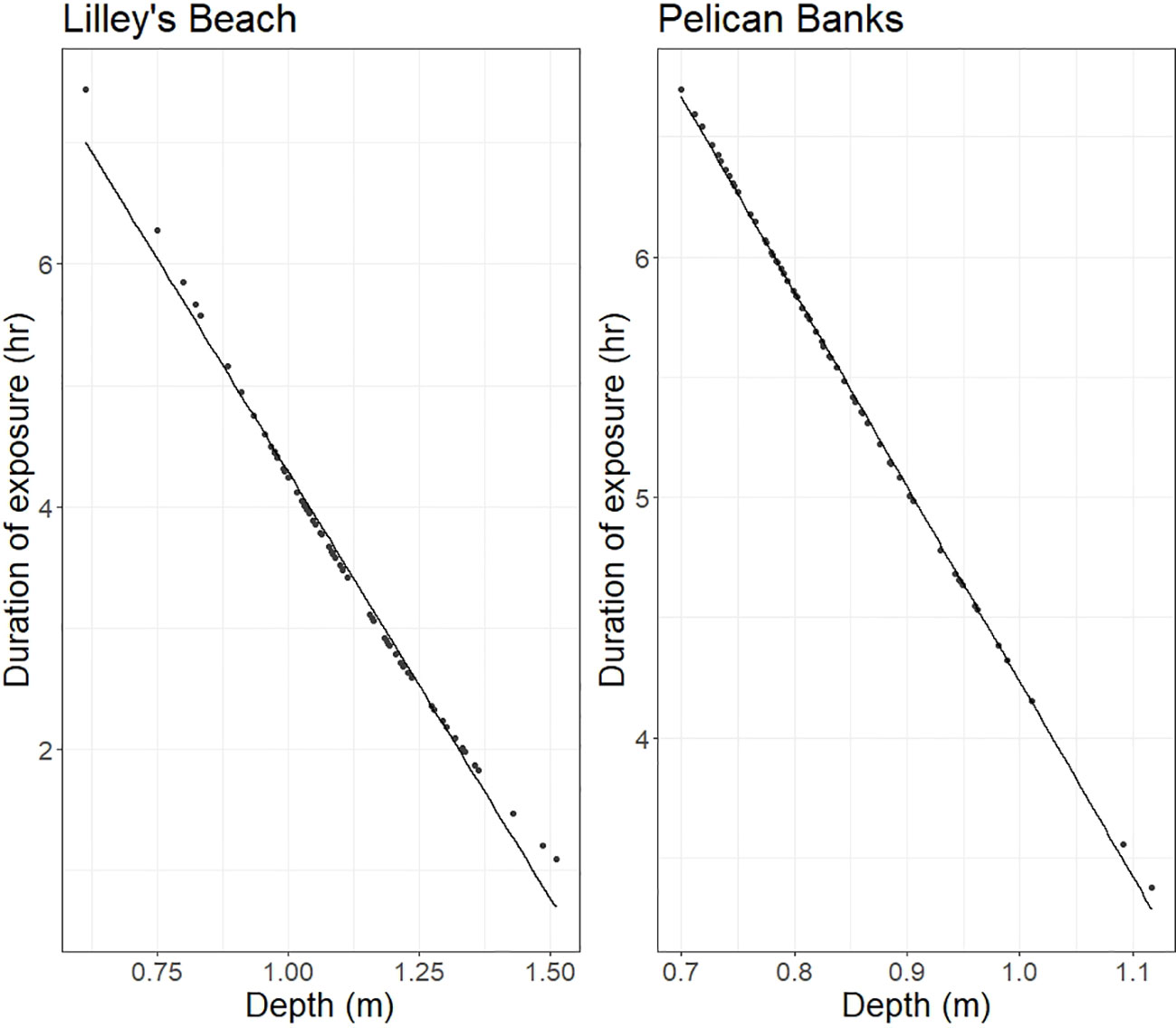
Figure 1 Relationship between the depth and exposure duration.
The percentage of plant cover exhibited high variability throughout the flowering season and across different years at both sites (Supplementary Figure 2). A notably lower percentage of plant cover was observed at Lilley’s Beach compared to Pelican Banks. At Lilley’s Beach, the plant cover was not present in all exposure categories. For instance, there was no plant cover in the exposure category 5-6 hours (0.78-0.91 m) in the year 2020. Additionally, plant cover was absent for both years in the lowest exposure category of 0-1 hours (1.45-1.58 m) (Supplementary Figure 2). Conversely, at Pelican Banks, plant cover was present in nearly all exposure categories for both years, with the exception of the 3-4 hour category (1.05-1.18 m), which was absent in the year 2021 (Supplementary Figure 2).
Based on the 2020 data, the daily average temperature exhibited a seasonal pattern throughout the flowering season, with no significant differences observed among exposure categories in both sites (Supplementary Figure 3). However, the daily average light intensities exhibited some differences, with deeper depths having relatively low light intensities, while shallow depths had high light intensities (Supplementary Figure 4).
Flowering variability
Flowering occurred from July to December in both years, and there was high temporal variability in the abundance, ratio, and morphology of flowering observed at both sites (Figures 2–5). The best models describing the abundance and ratio of flowering were bivariate, including plant cover and exposure, which explained 39% of the density of flowering shoots, 36% of the density of spathes and 28% of the flowering frequency (Table 1; Supplementary Data Table 1). In contrast, the best model for the morphology of flowering was univariate, with plant cover explaining 40% of the variation in the average number of spathes per flowering shoot (Table 1). Both predictor variables (i.e., plant cover and exposure) had significant positive effects on all flowering metrics.
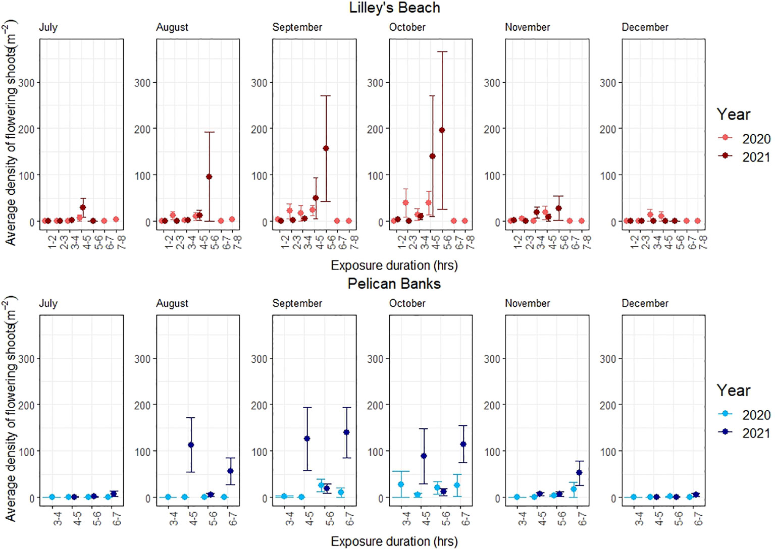
Figure 2 Variations in the density of flowering shoots. The line shows the standard error.
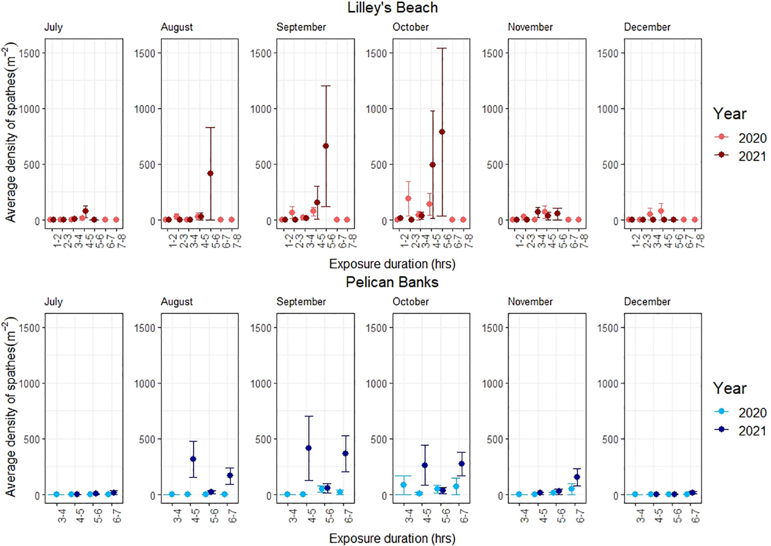
Figure 3 Variations in the density of spathes among exposure categories. The line shows the standard error.
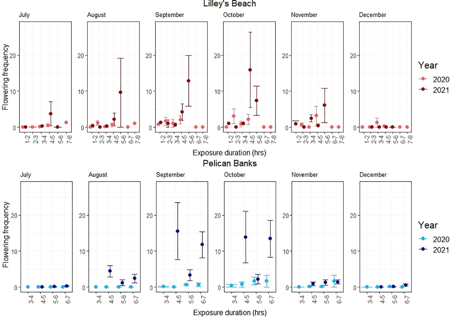
Figure 4 Variations in the flowering frequency among exposure categories. The line shows the standard error.
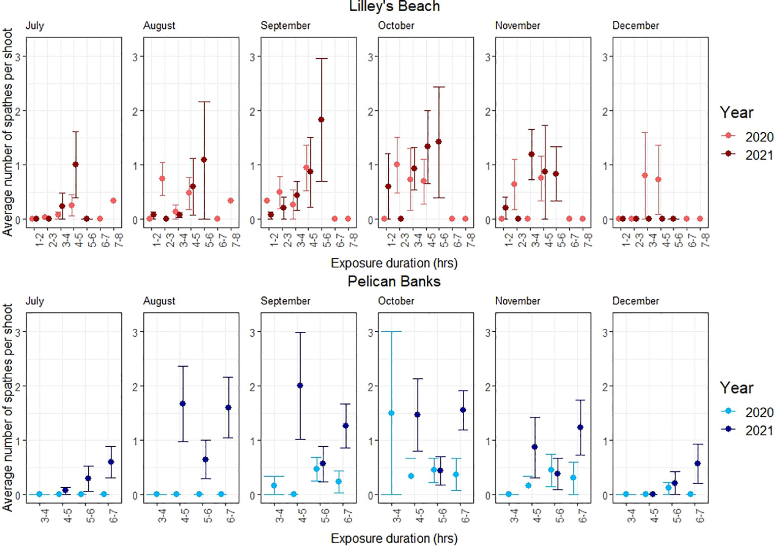
Figure 5 Variations in the average number of spathes per flowering shoots among exposure categories. The line shows the standard error.
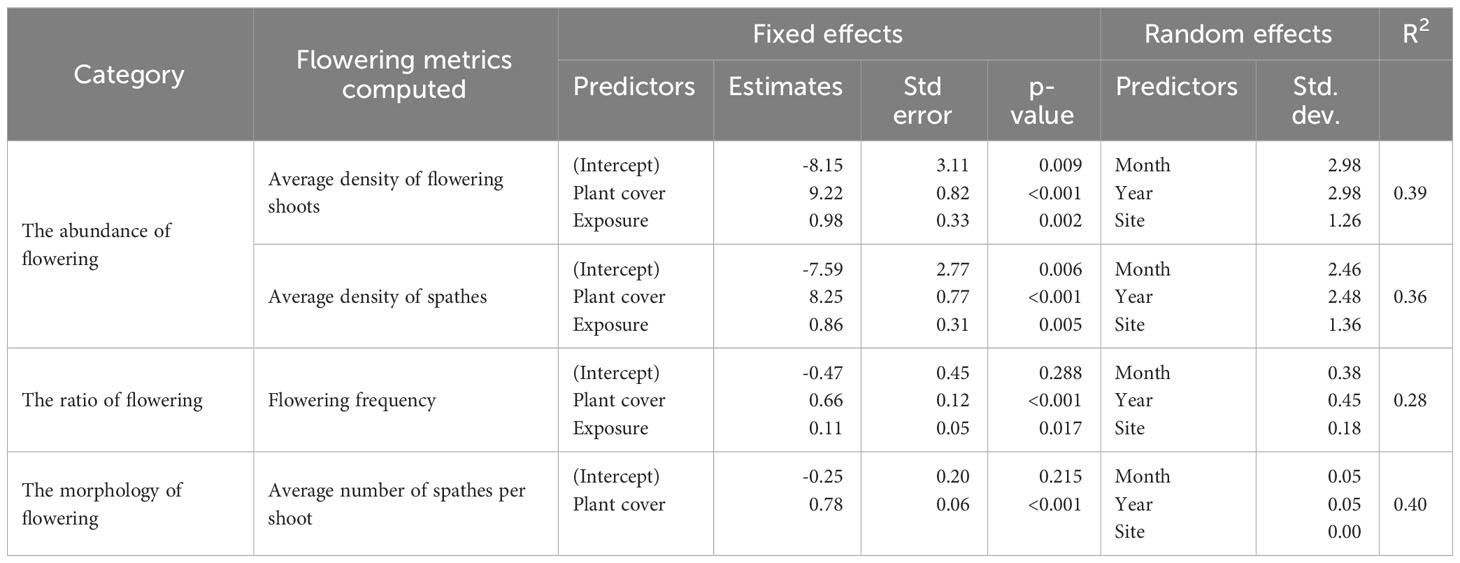
Table 1 Summary of the selected models of the abundance, ratio and morphology of flowering (significance level p<0.05).
The peak flowering was observed in September-October across most of the exposure categories in both sites (Figure 3). All flowering metrics showed a large variation between the two years, with a notable interannual variability noted only in Pelican Banks site (F120, 1 = 10.801, p<0.01, Table 2). Lilley’s Beach had a comparatively higher density of flowering shoots and spathe density than Pelican Banks, with the mean density of flowering shoots and spathe density reaching more than 196 m-2 and 600 m-2 during peak flowering months, respectively (Figures 2, 3). The frequency of flowering was relatively higher in most of the exposure categories in Lilley’s Beach than at the Pelican Banks over the flowering season (Figure 4).
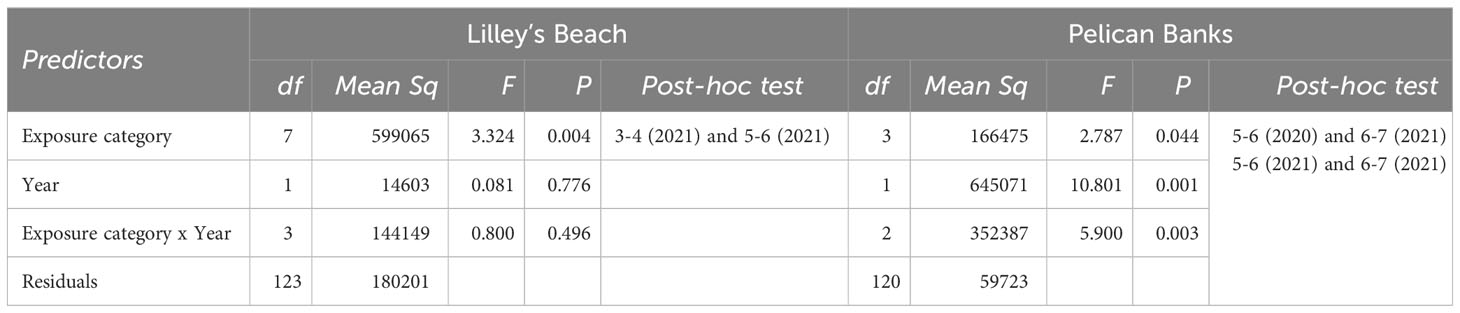
Table 2 Two-way ANOVA tests the differences in average spathe density in two sites (significance level p<0.01).
Additionally, the density of spathes was significantly different among exposure categories in Lilley’s Beach during the peak flowering months (F123, 7 = 3.324, p<0.01), where the difference was noted between 3-4 hrs and 5-6 hrs exposure categories in 2021 (post-hoc test, Table 2). The effect of the exposure duration was not prominent at the Pelican Banks site; however, a significant difference in spathe density resulted between 5-6 hrs and 6-7 hrs exposure categories in 2021 (Post-hoc test, Table 2). The depth gradient of this site was not as wide as Lilley’s Beach (Supplementary Figure 1). Significant inter-annual variation was observed only in Pelican Banks (F120, 1 = 10.801, p<0.01, Table 2) while the difference was noted between the same exposure categories (i.e., 5-6 hrs (2020) and 6-7 hrs (2021)) between years (Post-hoc test, Table 2).
Discussion
The study described here identified variability in the magnitude of flowering of Z. muelleri, a widely distributed species on the east coast of Australia. It further investigated the effects of exposure to elucidate the variabilities of flowering in intertidal meadows. Flowering was present and variable in both intertidal meadows studied, with the flowering season lasting approximately six months. Flowering was first observed in July in both meadows, and peak flowering is observed from September to October. The timing of Z. muelleri flowering from late winter to early summer is typical in most of the subtropical coasts of Australia (Unpublished data). Despite being located in the same climatic region, we observed a large variation in flowering over the flowering season in both meadows. By simultaneously conducting monthly sampling of these two meadows, we were able to capture the effects of exposure behind the variabilities of the abundance (measured as the density of flowering shoots and spathes), the ratio (measured as the flowering frequency), and the morphology of flowering (measured as the average number of spathes per flowering shoot) in this study.
Seagrasses were unequally distributed in both meadows, and the plant cover was highly variable over the flowering season. Similarly, the flowering was unequally distributed within the meadows. As we hypothesised, a large variation in the abundance and ratio of flowering was explained by plant cover and exposure together (approximately 39% of the density of flowering shoots, 36% of the density of spathes and 28% of flowering frequency). Similar variation in the morphology of flowering was explained by plant cover alone. The positive effect of plant cover in all flowering models indicated the plant’s resource investment towards flowering (Collier et al., 2014); however, its effect can be highly varied. For instance, we noted a considerably high abundance of flowering over the flowering season in some patches where seagrass was less dense, particularly in Lilley’s Beach. This might be due to the environmental stress during the exposure. Although the daily average temperature did not exceed the thermal optimum for gross photosynthesis of this species (31°C) (Collier et al., 2017) in our sites, seagrasses are likely to experience high light stress. We noted high daily average light intensities across the depth gradient, which are substantially higher than the optimum light levels required to protect at least 80%of shoots of the plant at cold temperatures (~3000 lux) when flowering is expected to trigger (Collier et al., 2016; Lekammudiyanse et al., 2023). As proposed by previous studies, Lilley’s Beach is also likely to experience stress from high wave energy due to its exposed position, where the wave energy was estimated as twice as high as Pelican Banks (Andrews et al., 2023). When a stress is present, plants tend to invest more resources towards reproduction as a stress-responsive mechanism (Fonseca and Bell, 1998; Potouroglou et al., 2014). This was also noted in flowering frequency, where the fraction of flowering is relatively higher in this site. The effect of exposure was further evident in the ANOVA model, where the spathe density significantly differed among 3-4 hrs and 5-6 hrs exposure categories in Lilley’s Beach during peak flowering in 2021. Such difference was noted in 5-6 hrs and 6-7 hrs exposure categories in Pelican Banks in 2021, however, the difference wasn’t highlighted in our model, probably due to a limited number of exposure categories that could not capture the differences in spathe densities.
Additionally, in Pelican Banks site, we noted a significant inter-annual variation in spathe density during the peak flowering times, with the spathe density being significantly higher in the second year. This difference might be due to the influence of other environmental drivers, such as the differences in small-scale local environmental conditions (e.g., nutrient content, temperature) and/or plant age (Cook, 1983; Johnson et al., 2017). Although, we could not compare the inter-annual differences in water temperature and light intensities in this study, changes in climatic variables, particularly temperature, could be an important factor that shapes the flowering cycle (Blok et al., 2018). Inter-annual variations could also be related to the plant’s age, as the plant’s flowering potential is supposed to exhibit an unimodal response with ramet’s maturity, and the relatively high abundance of flowering recorded in the second year could also be a reflection of plant age (Furman et al., 2015). In addition, the differences in plant’s phenotypic plasticity could also influence the flowering variabilities. For instance, in Lilley’s Beach, we observed a substantially high density of flowering shoots and spathes at intermediate depths during peak flowering months. Plants on Lilley’s Beach have different morphological characteristics (e.g., leaf length and width) relative to the Pelican Banks site (Andrews et al., 2023). Such adaptations can be expected even within the same climatic region due to the degree of local environmental stresses (e.g., sedimentation and high wave exposure) (Guerrero-Meseguer et al., 2021).
Our study provides practical information to help inform seed-based restoration projects conducted in subtropical intertidal meadows in Australia. While most of the restoration to date has been typically based on transplanting vegetative shoots, the most recent focus is extended towards either a combination of transplanting and seed-based restoration or entirely based on seed-based restoration due to the high success rates (Leschen et al., 2010; Orth et al., 2012; Infantes et al., 2016). For instance, seed-based restoration alone was found to extend the meadow by more than ten times during a decade in the coastal bays of Virginia in the USA (Orth et al., 2012). Restoration projects using seeds require site-specific knowledge of flowering strategies to identify the optimum harvesting time. As noted in this study, the September-October period is likely to generally be the optimum time for seed collection in subtropical meadows, though local spatial variability may affect the reliability of collection volumes. The spathe density in peak flowering months is likely to be influenced by exposure duration; however, this might not be a limiting factor in collecting flowers in meadows with narrow depth gradients unless the areas are preserved for self-re-establishment. We observed a relatively high number of flowers at intermediate depths than shallow or deep depths, where a high seed bank density might be expected (Olesen et al., 2017). Therefore, intermediate depths might be important for maintaining the resilience of the meadow when the re-establishment is dominated by sexual reproduction following disturbances (Kilminster et al., 2015). The spathe density reported in our study was substantially higher than previous records (Smith et al., 2016); however, the high density of flowering shoots/spathes may not reflect the production of viable seeds. Further studies will require assessing seed viability in different depths to ensure effective restoration (Vanderklift et al., 2020).
In this study, we were unable to count the number of spathes in each flowering shoot in every quadrat due to a large number of flowering shoots recorded in some quadrats and time restrictions, which is a limitation of the study. We estimated the total number of spathes based on the average number of spathes per flowering shoot in each quadrat, which may be subject to variation. Since we have a large sample size, we assumed that the variations are accounted in our analysis of the density of spathes. In future it will be beneficial to apply new technologies and associated optical imaging systems in monitoring seagrass flowering (e.g., drones). Additionally, we were unable to install loggers to download full record of temperature and light data in the second year due to the logger malfunctioning caused by frequent turtle bites, which is another limitation of this study. Furthermore, we did not count the number of seeds produced per spathe and their viability, which is another limitation we identified. However, in another preliminary study conducted along with these field surveys, it was shown that the viability of seeds and seed banks were not substantially different among exposure categories (Unpublished data). Further studies are required to understand the persistence of local seed banks of each subpopulation.
In summary, this study reported flowering intensities along the depth gradient in two subtropical intertidal meadows in Australia. The findings emphasized that the abundance and ratio of flowering can vary based on exposure duration. Also, the spathe density is highest in mid-Austral spring, which would be the best time to collect flowers. This study contributes to our understanding of meadow capacity for re-establishment at different intertidal depths and provides insights for seed-based restoration. Such habitat-specific studies are important for understanding local adaptation and resilience under climate change consequences (Tan et al., 2020).
Data availability statement
The original contributions presented in the study are included in the article/Supplementary Material. Further inquiries can be directed to the corresponding author.
Author contributions
ML designed and performed the fieldwork, analysed the data, prepared figures and tables and wrote the manuscript. EJ guided experimental design, and MS guided statistical analysis. EJ, MS, NF and AI contributed to revise the draft. All authors contributed to the article and approved the submitted version.
Funding
ML was supported by Central Queensland University International Excellence Scholarship, Australian Government Research Training Program Scholarship and CSIRO Postgraduate Scholarship (top-up scholarship and operating budget). MS was supported by a Julius Career Award from CSIRO.
Acknowledgments
We thank the Coastal Marine Ecosystems Research Centre, CQUniversity, for providing the field vessel and gear. We also thank R. Mulloy and M. Pfeiffer for assisting in the fieldwork.
Conflict of interest
The authors declare that the research was conducted in the absence of any commercial or financial relationships that could be construed as a potential conflict of interest.
Publisher’s note
All claims expressed in this article are solely those of the authors and do not necessarily represent those of their affiliated organizations, or those of the publisher, the editors and the reviewers. Any product that may be evaluated in this article, or claim that may be made by its manufacturer, is not guaranteed or endorsed by the publisher.
Supplementary material
The Supplementary Material for this article can be found online at: https://www.frontiersin.org/articles/10.3389/fmars.2023.1195084/full#supplementary-material
References
Andrews E. L., Irving A. D., Sherman C. D., Jackson E. L. (2023). Spatio-temporal analysis of the environmental ranges and phenotypic traits of Zostera muelleri subpopulations in Central Queensland. Estuarine Coast. Shelf Sci. 281, 108191. doi: 10.1016/j.ecss.2022.108191
Blok S., Olesen B., Krause-Jensen D. (2018). Life history events of eelgrass Zostera marina L. populations across gradients of latitude and temperature. Mar. Ecol. Prog. Ser. 590, 79–93. doi: 10.3354/meps12479
Boese B. L., Alayan K. E., Gooch E. F., Robbins B. D. (2003). Desiccation index: a measure of damage caused by adverse aerial exposure on intertidal eelgrass (Zostera marina) in an Oregon (USA) estuary. Aquat. Bot. 76, 329–337. doi: 10.1016/S0304-3770(03)00068-8
Burnham K. P., Anderson D. R. (2004). Multimodel inference: understanding AIC and BIC in model selection. Sociological Methods Res. 33, 261–304. doi: 10.1177/0049124104268644
Cabaço S., Machas R., Santos R. (2009). Individual and population plasticity of the seagrass Zostera noltii along a vertical intertidal gradient. Estuar. Coast. Shelf Sci. 82 (2), 301–308. doi: 10.1016/j.ecss.2009.01.020
Campey M. L., Kendrick G. A., Walker D. I. (2002). Interannual and small-scale spatial variability in sexual reproduction of the seagrasses Posidonia coriacea and Heterozostera tasmanica, southwestern Australia. Aquat. Bot. 74, 287–297. doi: 10.1016/S0304-3770(02)00127-4
Clavier J., Chauvaud L., Carlier A., Amice E., van der Geest M., Labrosse P., et al. (2011). Aerial and underwater carbon metabolism of a Zostera noltii seagrass bed in the Bancd’Arguin, Mauritania. Aquat. Bot. 95, 24–30. doi: 10.1016/j.aquabot.2011.03.005
Collier C., Adams M., Langlois L., Waycott M., O’brien K., Maxwell P., et al. (2016). Thresholds for morphological response to light reduction for four tropical seagrass species. Ecol. Indic. 67, 358–366. doi: 10.1016/j.ecolind.2016.02.050
Collier C. J., Ow Y. X., Langlois L., Uthicke S., Johansson C. L., O’Brien K. R., et al. (2017). Optimum temperatures for net primary productivity of three tropical seagrass species. Front. Plant Sci. 8, 1446. doi: 10.3389/fpls.2017.01446
Collier C. J., Villacorta-Rath C., Van Dijk K. J., Takahashi M., Waycott M. (2014). Seagrass proliferation precedes mortality during hypo-salinity events: a stress-induced morphometric response. PloS One 9, e94014. doi: 10.1371/journal.pone.0094014
Conacher C., Poiner I., O’donohue M. (1994). Morphology, flowering and seed production of Zostera capricorni Aschers. in subtropical Australia. Aquat. Bot. 49, 33–46. doi: 10.1016/0304-3770(94)90004-3
Cook R. E. (1983). Clonal plant populations: A knowledge of clonal structure can affect the interpretation of data in a broad range of ecological and evolutionary studies. Am. scientist 71, 244–253. Available at: https://www.jstor.org/stable/27852011.
de Fouw J., Govers L. L., Van De Koppel J., Van Belzen J., Dorigo W., Cheikh M., et al. (2016). Drought, mutualism breakdown, and landscape-scale degradation of seagrass beds. Curr. Biol. 26, 1051–1056. doi: 10.1016/j.cub.2016.02.023
Fonseca M. S., Bell S. S. (1998). Influence of physical setting on seagrass landscapes near Beaufort, North Carolina, USA. Mar. Ecol. Prog. Ser. 171, 109–121. doi: 10.3354/meps171109
Furman B. T., Jackson L. J., Bricker E., Peterson B. J. (2015). Sexual recruitment in Zostera marina: A patch to landscape-scale investigation. Limnology Oceanography 60, 584–599. doi: 10.1002/lno.10043
Guerrero-Meseguer L., Veiga P., Sampaio L., Rubal M. (2021). Sediment characteristics determine the flowering effort of Zostera noltei meadows inhabiting a human-dominated lagoon. Plants 10, 1387. doi: 10.3390/plants10071387
Harrison P. G. (1982). Spatial and temporal patterns in abundance of two intertidal seagrasses, Zostera americana Den Hartog and Zostera marina L. Aquat. Bot. 12, 305–320. doi: 10.1016/0304-3770(82)90024-9
Henderson J., Hacker S. D. (2015). Buried alive: an invasive seagrass (Zostera japonica) changes its reproductive allocation in response to sediment disturbance. Mar. Ecol. Prog. Ser. 532, 123–136. doi: 10.3354/meps11335
Infantes E., Eriander L., Moksnes P. O. (2016). Eelgrass (Zostera marina) restoration on the west coast of Sweden using seeds. Mar. Ecol. Prog. Ser. 546, 31–45. doi: 10.3354/meps11615
Infantes E., Moksnes P. O. (2018). Eelgrass seed harvesting: Flowering shoots development and restoration on the Swedish west coast. Aquat. Bot. 144, 9–19. doi: 10.1016/j.aquabot.2017.10.002
Inglis G. J., Smith M. P. L. (1998). Synchronous flowering of estuarine seagrass meadows. Aquat. Bot. 60, 37–48. doi: 10.1016/S0304-3770(97)00068-5
Jackson L. J., Furman B. T., Peterson B. J. (2017). Morphological response of Zostera marina reproductive shoots to fertilised porewater. J. Exp. Mar. Biol. Ecology 489, 1–6. doi: 10.1016/j.jembe.2017.01.002
Johnson A. J., Moore K. A., Orth R. J. (2017). The influence of resource availability on flowering intensity in Zostera marina (L.). J. Exp. Mar. Biol. Ecol. 490, 13–22. doi: 10.1016/j.jembe.2017.02.002
Kilminster K., Mcmahon K., Waycott M., Kendrick G. A., Scanes P., Mckenzie L., et al. (2015). Unravelling complexity in seagrass systems for management: Australia as a microcosm. Sci. Total Environ. 534, 97–109. doi: 10.1016/j.scitotenv.2015.04.061
Koch E. W. (2001). Beyond light: physical, geological, and geochemical parameters as possible submersed aquatic vegetation habitat requirements. Estuaries 24, 1–17. doi: 10.2307/1352808
Kutner M., Nachtsheim C., Neter J., Li W. (2004). Applied linear statistical models (Boston: McGraw-Hill).
Lekammudiyanse M. U., Saunders M. I., Flint N., Irving A. D., Jackson E. L. (2022). Simulated megaherbivore grazing as a driver of seagrass flowering. Mar. Environ. Res. 179, 105698. doi: 10.1016/j.marenvres.2022.105698
Lekammudiyanse M. U., Saunders M. I., Flint N., Irving A., Jackson E. L. (2023). Simulated effects of tidal inundation and light reduction on Zostera muelleri flowering in seagrass nurseries. Mar. Environ. Res. 188, 106010. doi: 10.1016/j.marenvres.2023.106010
Leschen A. S., Ford K. H., Evans N. T. (2010). Successful eelgrass (Zostera marina) restoration in a formerly eutrophic estuary (Boston Harbor) supports the use of a multifaceted watershed approach to mitigating eelgrass loss. Estuaries coasts 33, 1340–1354. doi: 10.1007/s12237-010-9272-7
Leuschner C., Landwehr S., Mehlig U. (1998). Limitation of carbon assimilation of intertidal Zostera noltii and Z. marina by desiccation at low tide. Aquat. Bot. 62, 171–176. doi: 10.1016/S0304-3770(98)00091-6
Mony C., Puijalon S., Bornette G. (2011). Resprouting response of aquatic clonal plants to cutting may explain their resistance to spate flooding. Folia Geobotanica 46, 155–164. doi: 10.1007/s12224-010-9095-0
Nelson C. R., Halpern C. B., Antos J. A. (2007). Variation in responses of late-seral herbs to disturbance and environmental stress. Ecology 88, 2880–2890. doi: 10.1890/06-1989.1
Olesen B., Krause-Jensen D., Christensen P. B. (2017). Depth-related changes in reproductive strategy of a cold-temperate Zostera marina meadow. Estuaries Coasts 40, 553–563. doi: 10.1007/s12237-016-0155-4
Orth R. J., Moore K. A., Marion S. R., Wilcox D. J., Parrish D. B. (2012). Seed addition facilitates eelgrass recovery in a coastal bay system. Mar. Ecol. Prog. Ser. 448, 177–195. doi: 10.3354/meps09522
Peterken C. J., Conacher C. A. (1997). Seed germination and recolonisation of Zostera capricorni after grazing by dugongs. Aquat. Bot. 59, 333–340. doi: 10.1016/S0304-3770(97)00061-2
Potouroglou M., Kenyon E. J., Gall A., Cook K. J., Bull J. C. (2014). The roles of flowering, overwinter survival and sea surface temperature in the long-term population dynamics of Zostera marina around the Isles of Scilly, UK. Mar. pollut. Bull. 83, 500–507. doi: 10.1016/j.marpolbul.2014.03.035
Ralph P., Durako M. J., Enriquez S., Collier C., Doblin M. (2007). Impact of light limitation on seagrasses. J. Exp. Mar. Biol. Ecol. 350, 176–193. doi: 10.1016/j.jembe.2007.06.017
Ramage D. L., and Schiel D. R. (1998). Reproduction in the seagrass Zostera novazelandica on intertidal platforms in southern New Zealand. Mar. Biol. 130, 479–489. doi: 10.1007/s002270050268
Rasheed M. A. (1999). Recovery of experimentally created gaps within a tropical Zostera capricorni (Aschers.) seagrass meadow, Queensland, Australia. J. Exp. Mar. Biol. Ecol. 235 (2), pp.183–pp.200. doi: 10.1016/S0022-0981(98)00158-0
Rasheed M. A. (2004). Recovery and succession in a multi-species tropical seagrass meadow following experimental disturbance: the role of sexual and asexual reproduction. J. Exp. Mar. Biol. Ecol. 310, 13–45. doi: 10.1016/j.jembe.2004.03.022
Rufino M. M., Bez N., Brind’amour A. (2018). Integrating spatial indicators in the surveillance of exploited marine ecosystems. PLoS One 13, e0207538. doi: 10.1371/journal.pone.0207538
Seagrass-Watch (2023) Percent cover standards - Estuary, Zostera, Seagrass-Watch, Australia. Available at: https://www.seagrasswatch.org/manuals/ (Accessed 12 July 2022).
Silva J., Santos R. (2003). Daily variation patterns in seagrass photosynthesis along a vertical gradient. Mar. Ecol. Prog. Ser. 257, 37–44. doi: 10.3354/meps257037
Smith T. M., York P. H., Macreadie P. I., Keough M. J., Ross D. J., Sherman C. D. (2016). Spatial variation in reproductive effort of a southern Australian seagrass. Mar. Environ. Res. 120, 214–224. doi: 10.1016/j.marenvres.2016.08.010
Tan Y. M., Dalby O., Kendrick G. A., Statton J., Sinclair E. A., Fraser M. W., et al. (2020). Seagrass restoration is possible: insights and lessons from Australia and New Zealand. Front. Mar. Sci. 7, 617. doi: 10.3389/fmars.2020.00617
Team R. C. (2020). A Language and Environment for Statistical Computing. R Foundation for Statistical Computing (Vienna: Austria patent application).
Underwood A. J. (1997). Experiments in ecology: their logical design and interpretation using analysis of variance (Cambridge: Cambridge university press).
Vanderklift M. A., Doropoulos C., Gorman D., Leal I., Minne A. J., Statton J., et al. (2020). Using propagules to restore coastal marine ecosystems. Front. Mar. Sci. 724. doi: 10.3389/fmars.2020.00724
Vermaat J. E. (2009). Linking clonal growth patterns and ecophysiology allows the prediction of meadow-scale dynamics of seagrass beds. Perspect. Plant Ecology Evol. Systematics 11, 137–155. doi: 10.1016/j.ppees.2009.01.002
von Staats D. A., Hanley T. C., Hays C. G., Madden S. R., Sotka E. E., Hughes A. R. (2021). Intra-meadow variation in seagrass flowering phenology across depths. Estuaries Coasts 44, 325–338. doi: 10.1007/s12237-020-00814-0
Wang M., Zhang H., Tang X. (2019). Biotic and abiotic conditions can change the reproductive allocation of Zostera marina inhabiting the coastal areas of North China. J. Ocean Univ. China 18 (2), 528–536. doi: 10.1007/s11802-019-3796-7
Keywords: seagrass flowering, plant cover, intertidal depth, exposure duration, Zostera muelleri
Citation: Lekammudiyanse MU, Saunders MI, Flint N, Irving A and Jackson EL (2023) Flowering variabilities in subtropical intertidal Zostera muelleri meadows of Australia. Front. Mar. Sci. 10:1195084. doi: 10.3389/fmars.2023.1195084
Received: 28 March 2023; Accepted: 11 September 2023;
Published: 04 October 2023.
Edited by:
Ronald Osinga, Wageningen University and Research, NetherlandsReviewed by:
Kathryn Margaret McMahon, Edith Cowan University, AustraliaJennifer Li Ruesink, University of Washington, United States
W. Judson Kenworthy, Independent Researcher, Beaufort, NC, United States
Copyright © 2023 Lekammudiyanse, Saunders, Flint, Irving and Jackson. This is an open-access article distributed under the terms of the Creative Commons Attribution License (CC BY). The use, distribution or reproduction in other forums is permitted, provided the original author(s) and the copyright owner(s) are credited and that the original publication in this journal is cited, in accordance with accepted academic practice. No use, distribution or reproduction is permitted which does not comply with these terms.
*Correspondence: Manuja U. Lekammudiyanse, bS5sZWthbW11ZGl5YW5zZUBjcXVtYWlsLmNvbQ==