Modeling the effects of large-scale interior headland restoration on tidal hydrodynamics and salinity transport in an open coast, marine-dominant estuary

The effects of large-scale interior headland restoration on tidal hydrodynamics and salinity transport in an open coast, marine dominant estuary (Grand Bay, Alabama, U.S.A) are investigated using a two-dimensional model, the Discontinuous-Galerkin Shallow Water Equations Model (DG-SWEM). Three restoration alternatives are simulated for present-day conditions, as well as under 0.5 m of sea level rise (SLR). Model results show that the restoration alternatives have no impact on tidal range within the estuary but change maximum tidal velocities by ±5 cm/s in the present-day scenarios and by ±7 cm/s in the scenarios with 0.5 m of SLR. Differences in average salinity concentrations for simulated tropical and frontal seasons show increases and decreases on the order of 2 pss in the embayments surrounding the restoration alternatives; differences were larger (on the order of ±4 pss) for the scenarios with 0.5 m of SLR. There were minimal changes in average salinity outside of the estuary and no changes offshore. The size and position of the alternatives played a role in the salinity response as a result of changing the estuarine shoreline geometry and affecting the fetch within the bay. SLR was more impactful in increasing exposure to low salinity values (i.e., less than 5 pss) than the presence of the restoration alternatives. Overall, the modeled results indicate that these large-scale restoration actions have limited and localized impacts on the hydrodynamics and salinity patterns in this open coast estuary. The results also demonstrate the nonlinear response of salinity to SLR, with increases and decreases in the maximum, mean and minimum daily salinity concentrations from present-day conditions. This nonlinear response was a result of changes in the directions of the residual currents, which affected salinity transport.

1 Introduction

Coastal estuaries are economically and ecologically significant environments that support diverse habitats and provide a range of ecosystem services to human communities including protection during storm events. Climate change and sea level rise (SLR) in particular have the potential to alter the hydrodynamic processes that govern coastal ecosystems and habitats for a variety of species (Passeri et al., 2016, Alizad et al., 2018, Xie et al., 2020). The effects of SLR are particularly pronounced on low-gradient coastlines like the northern Gulf of Mexico where higher water levels can penetrate further inland (Passeri et al., 2015). In coastal estuaries, SLR can nonlinearly increase tidal ranges, tidal prisms, tidal velocities and alter sediment transport patterns (French, 2008; Leorri et al., 2011; Pickering et al., 2012; Hall et al., 2013; Pelling et al., 2013; Valentim et al., 2013; Arns et al., 2015; Passeri et al., 2016; Xie et al., 2022). Additionally, SLR allows greater amounts of saline water to enter estuaries, resulting in higher salinity ranges (Huang et al., 2015). Like hydrodynamics, salinity response to SLR is nonlinear; previous work has shown that salinity under future SLR may be 20-50% higher than present-day conditions in coastal estuaries (Mulamba et al., 2019). Further, a previous modeling study found that under 0.2 m of SLR, bay-averaged salinity increased by 0.5 on the practical salinity scale (pss) (Hilton et al., 2008). Changes in salinity can have adverse outcomes for the ecology of coastal systems. For example, salt marshes are governed by tidal inundation, salinity and sediment supply (Alizad et al., 2016, Alizad et al., 2018, Ganju et al., 2019). Ecological processes are moderated by coastal salinity ranges, particularly extreme values of salinity, which can affect the viability of species such as oysters (Yurek et al., 2023).

Coastal ecosystem restoration has been used to reestablish the ecological function and services of declining coastal and marine habitats. There is an increasing interest in large-scale restoration efforts that combine remediation of degraded ecosystems due to past impacts with adaptation to future threats such as climate change (Abelson et al., 2020). Sediment is a critical natural resource that can be used to achieve conservation and restoration initiatives in coastal systems (Parson and Swafford, 2012; Miselis et al., 2021). In the northern Gulf of Mexico, beneficial use of dredged sediments has been used as a way to keep sediment within the natural system to improve environmental conditions, provide storm damage protection and contribute to habitat creation and restoration goals (Parson and Swafford, 2012; King et al., 2020; Suedel et al., 2021). One area of interest for beneficial use of dredged sediments is Grand Bay, an open coast, marine-dominant estuary that is located within the Mississippi Sound at the border of Mississippi and Alabama (Figure 1). Grand Bay is separated from the Gulf of Mexico by Mobile Bay to the east, and a series of offshore barrier islands. The estuary contains embayments on the Mississippi and Alabama side, tidal creeks and an extensive salt marsh system. The bays are shallow with average water depths ranging from 0.5 m to 3.0 m (Peterson et al., 2007). Currently, the estuary does not have a fluvial source, and hydrodynamics are primarily driven by tides and winds. Tides are microtidal (range less than 1 m). Within the bays, winds modify water levels and currents, whether from daily sea breezes or stronger frontal and tropical events (Nowacki and Ganju, 2020). The estuary supports recreational and commercial fisheries with an abundance of marine life including shrimp, crabs and oysters (Eleuterius and Criss, 1991). Since the mid-1800s, high rates of shoreline erosion (between -0.50 m/year and -3.39 m/year (Terrano, 2018)) have led to the degradation of interior headlands within the estuary including Grand Batture Island, Isles aux Dames and Marsh Island (Figure 1). Coastal managers are exploring restoration actions to increase estuarine resilience including reconstructing the degraded interior headlands on the Alabama side of the estuary with dredged sediments. However, management decision-making relies on scientific evaluations to assess the impacts of large-scale restoration efforts on broader estuarine hydrodynamics and water quality (salinity) in order to understand potential changes to ecosystems including seagrass beds that surround the remnant Grand Batture shoals and oysters on the eastern shoreline near Isle aux Dames.

FIGURE 1

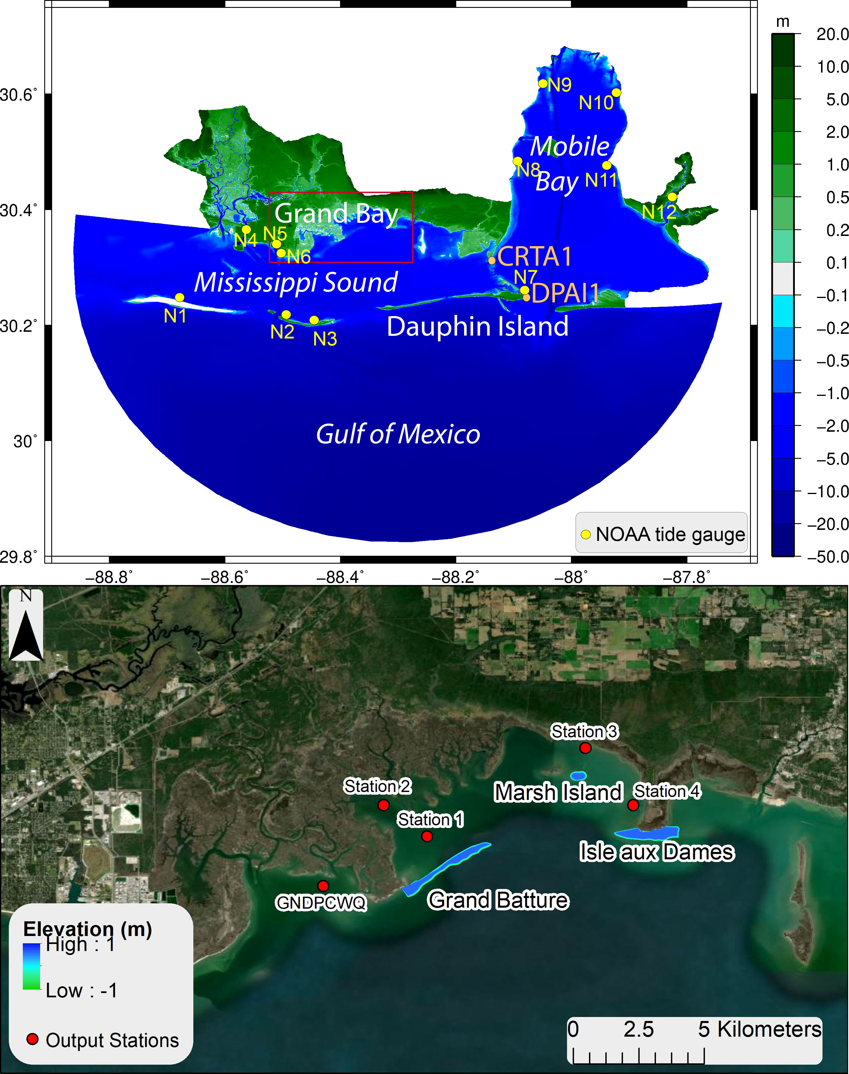
Figure 1 MSAL model domain and grid elevations with locations of National Data Buoy Center (NDBC) stations CRTA1 (Cedar Point, AL) and DPAI1 (Dauphin Island, AL) and National Oceanic and Atmospheric Administration (NOAA) tide gauge stations N1 – N12 (top); Inset of Grand Bay estuary with restoration alternatives and model output stations for MSAL salinity simulations (bottom).

This study assesses the impacts of a proposed large-scale restoration effort, namely interior headland restoration, on tidal hydrodynamics and salinity transport in an open coast, marine dominant estuary in Grand Bay, AL. A two-dimensional numerical model was developed to simulate hydrodynamics and salinity transport, with and without the proposed restoration. The results of the study provide insight into how large-scale restoration can alter the physical estuarine processes under present-day conditions as well as future SLR.

2 Methodology

2.1 Restoration alternatives

The purpose of restoring the interior headlands within the estuary to their historic footprint is to increase estuarine resilience (e.g., reducing shoreline erosion) while not creating adverse effects for ecosystems. Three restoration alternatives were considered: 1) no-action (no restoration occurs and the system evolves naturally); 2) reconstruction of the Grand Batture Island (herein referred to as GBI); and 3) reconstruction of the Grand Batture Island, Isle aux Dames and Marsh Island (herein referred to as All Alternatives). The proposed reconstructed islands and headlands are sandy features that are low in elevation (less than 1 m). Their footprint covers the historic (circa 1848) shoreline positions that existed on the Alabama side of the estuary (Figure 1). Grand Batture Island is the largest of the features, at approximately 3500 m in alongshore length and 350 m in cross-shore length. Its position changes the geometry of the shoreline and creates a semi-enclosed bay. Isle aux Dames broadens the existing headland, increasing the alongshore length to approximately 2500 m and the cross-shore width to 350 m. Marsh Island is a small feature positioned in the middle of the bay that is approximately 500 m in alongshore length and 350 m in cross-shore width.

2.2 Model description

To simulate hydrodynamics and salinity transport, the Discontinuous-Galerkin Shallow Water Equations Model (DG-SWEM) was used. DG-SWEM is a two-dimensional (2D) model that solves the depth-integrated shallow water equations and depth-averaged transport equation for the simulation of hydrodynamics (water surface elevations and currents) and salinity transport using discontinuous-Galerkin methods within the ADCIRC framework (Luettich et al., 1992; Kubatko et al., 2006). An unstructured finite element mesh was adapted for the localized region of coastal Mississippi/Alabama from a previously validated large-scale ADCIRC model (Bilskie et al., 2016). The modified mesh includes the Gulf of Mexico (open ocean boundary) and Mississippi Sound, with higher spatial resolution elements (on the order of 20 m) incorporated in the Grand Bay estuary (herein referred to as the MSAL model; Figure 1). Bathymetric and topographic elevations were derived from a digital elevation model (DEM) constructed with lidar data, National Ocean Service (NOS) hydrographic surveys, U.S. Army Corps of Engineers (USACE) channel surveys and the National Oceanographic and Atmospheric Administration (NOAA) nautical charts to represent present-day conditions (see Bilskie et al., 2016 for details). Within the marsh regions of Grand Bay, an elevation correction based on biomass density was used to adjust lidar-derived elevations due to the inability of lidar to penetrate marsh grass and correctly measure the elevation of the marsh platform (Medeiros et al., 2015; Alizad et al., 2020). This technique uses ASTER (Advanced Spaceborne Thermal Emissions and Reflection Radiometer) and IfSAR (interferometric synthetic aperture radar) satellite imagery along with lidar-derived canopy heights to classify the above-ground biomass density as high, medium or low. The biomass density class is then used to lower the DEM.

Salinity was initialized using data from Conductivity, Temperature, Depth (CTD) casts collected within Grand Bay in 2016 (Marot et al., 2019). The salinity profile of the water column was recorded at 26 sites from May 14 – May 18, 2016 (Figure 2), with depths ranging from 0.15 to 3.34 m. The range of observed salinity was 13.8 to 19.8 pss with an average standard deviation of 0.18 pss. Based on the salinity measurements, the estuary appears to be well-mixed with negligible vertical stratification. This supports the use of a 2D depth-integrated model to assess spatial changes in salinity.

FIGURE 2

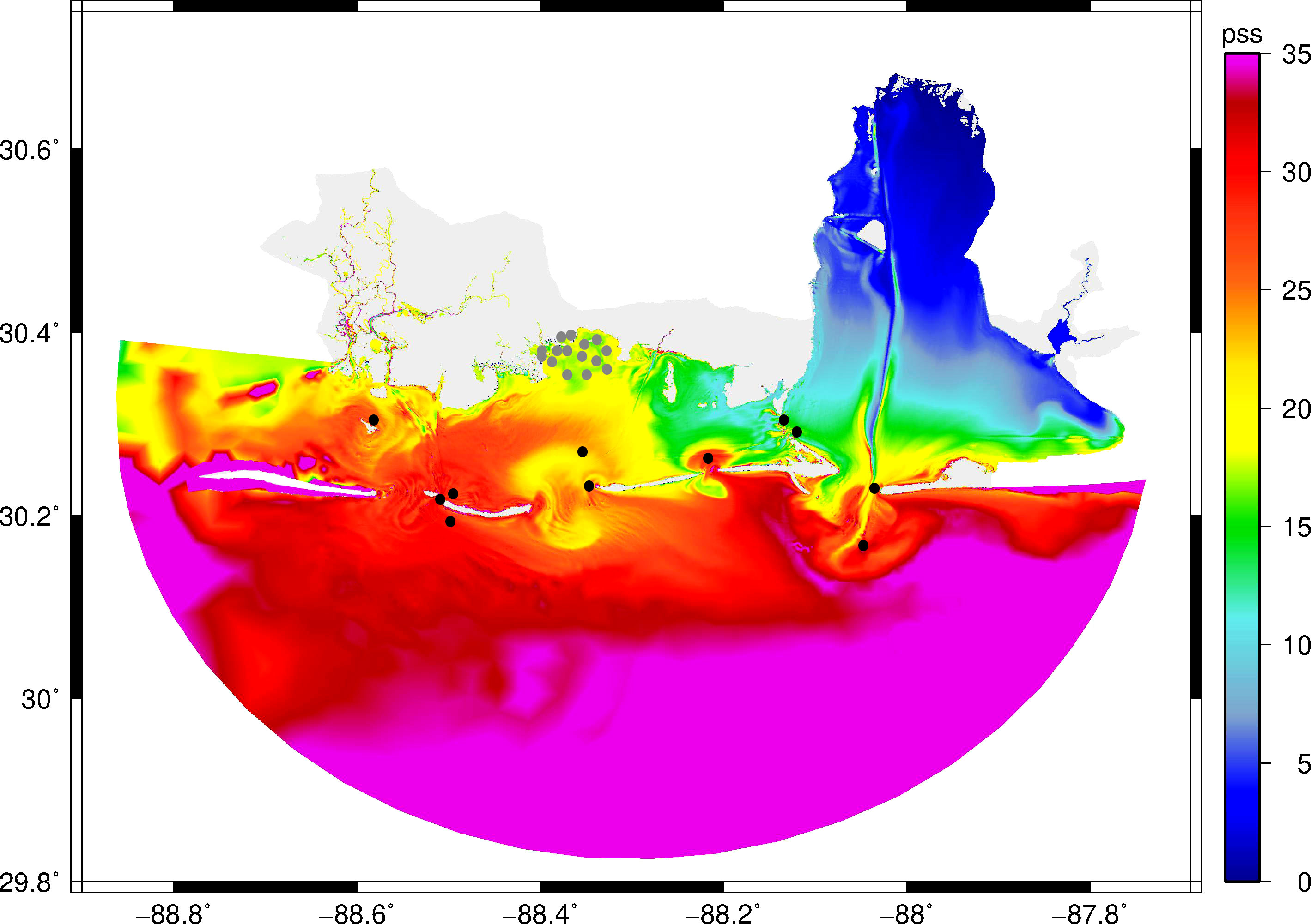
Figure 2 Initial salinity (pss; practical salinity scale) interpolated onto the model mesh. Black dots represent locations of NGOFS2 modeled salinity and grey dots represent locations of CTD casts in Grand Bay that were used to create the initial salinity.

The average salinity at each CTD cast was combined with forecasted salinity data from the NOAA Northern Gulf of Mexico Operational Forecast System (NGOFS2) to provide initial salinity conditions. The best available forecast data from NGOFS2 at the time of the study was extracted at various locations within the MSAL model domain throughout the Mississippi Sound, Mobile Bay and Gulf of Mexico, and averaged temporally over the collection period. The nodes of the offshore MSAL boundary were assumed to have salinity values of 36 pss representing an open-ocean salinity value; land nodes had values of 0 pss. Using these point-based measurements, kriging interpolation was used to create an initial salinity surface, which was then interpolated onto the MSAL model grid (Figure 2).

Additional DG-SWEM model parameters and settings include spatially varying quadratic bottom friction using the Manning’s roughness formulation, nonlinear advection, nonlinear finite amplitude effects, wetting and drying, horizontal eddy viscosity of 20 m²/s and a spatially varying Coriolis parameter. The model was run with a timestep of 1 s.

2.3 Model forcing

To provide boundary conditions for the MSAL model, the previously developed and validated 2D large-scale ADCIRC NGOM-RT model was used (Bilskie et al., 2020). The NGOM-RT unstructured finite element mesh encompasses the Western North Atlantic Tidal model domain west of the 60°W meridian (open ocean boundary), including the Caribbean Sea and the Gulf of Mexico. Higher spatial resolution elements (on the order of 20–100 m) are incorporated in the northern Gulf of Mexico (NGOM) coast across Mississippi, Alabama and the Florida panhandle coastal floodplain. The model has been validated for astronomic tides and hurricane storm surge simulations for hurricanes Ivan (2004), Dennis (2005), Katrina (2005) and Isaac (2012). For details on model development and validation, see Bilskie et al. (2020). In this study, NGOM-RT was used to force the MSAL model with hourly timeseries of water levels at the locations of the open-ocean boundary nodes. To simulate astronomic tides, NGOM-RT was forced with water surface elevations of eight harmonic constituents (K₁, O₁, M₂, S₂, N₂, K₂, Q₁, and P₁) along the open ocean boundary (Egbert et al., 1994; Egbert and Erofeeva, 2002). For salinity transport simulations that included meteorological forcing, NGOM-RT was hot-started from a 14-day tide spinup. Meteorological forcing was obtained from the NOAA National Centers for Environmental Prediction (NCEP) North American Mesoscale Forecast System (NAM), which models regional winds and pressures at a 12 km spatial scale and a 6-hour temporal scale. Details on MSAL model simulations can be found in Section 2.4 and Section 2.5.

2.4 Model validation

Validation of the MSAL model was done in two parts: 1) a tidal hydrodynamic validation and 2) a salinity transport validation. For the tidal validation, astronomic tides were simulated for 45 days beginning from a cold start with a 10-day ramp using a hyperbolic tangent function, followed by 5 days of dynamic steady state. 23 modeled tidal constituents were analyzed over the last 30 days of the simulation and compared with recorded tidal constituents at 12 NOAA tide gauge stations within the model domain (Figure 1; https://tidesandcurrents.noaa.gov). A tidal resynthesis of the measured and observed constituents for the first spring-neap cycle of a tidal epoch (~14.7 days) at each of the tide gauge stations was performed. For brevity, the tidal resynthesis at four stations is shown in Figure 3; these stations were selected based on their proximity (both near and far) to the study area. The modeled tidal signals match well in amplitude and phase, particularly at stations located along the offshore barrier islands (e.g., N2, N7 in Figure 1) and close to Grand Bay (e.g., N6 in Figure 1). The stations with the largest deviations (e.g., N10 in Figure 1) are located in Mobile Bay. The average root mean square error (RMSE) in the water levels at all stations is 0.06 m. In addition to the tidal resynthesis, a comparison of the modeled and observed amplitudes and phases for the five dominant constituents (K₁, O₁, M₂, Q₁, and S₂) at all stations is shown in Figure 4. Difference bands are plotted at ±0.025 and ±0.05 m in the amplitude plots, and ±10° and ±20° in the phase plots. The modeled constituent amplitudes at all stations fall within the 0.05 m difference band. The majority of the modeled phases of the three most dominant constituents (K₁, O₁, and M₂) fall within the 20° difference band. The largest deviations in phase occur for the S₂ and Q₁ constituents, particularly at the stations located in Mobile Bay. The discrepancies in the modeled amplitudes and phases are likely a result of the model grid only capturing the in-bank areas of Mobile Bay, and not the surrounding floodplain where low elevation wetlands may play a role in tidal propagation (e.g., as seen in the tidal resynthesis at the N10 station in Figure 3, which inaccurately predicts low tide). However, the contribution of these constituents to the tidal signal is minimal in comparison with K₁, O₁, and M₂ and inaccuracies in the tidal signal at gauges within Mobile Bay are not expected to affect the modeled hydrodynamics in Grand Bay.

FIGURE 3

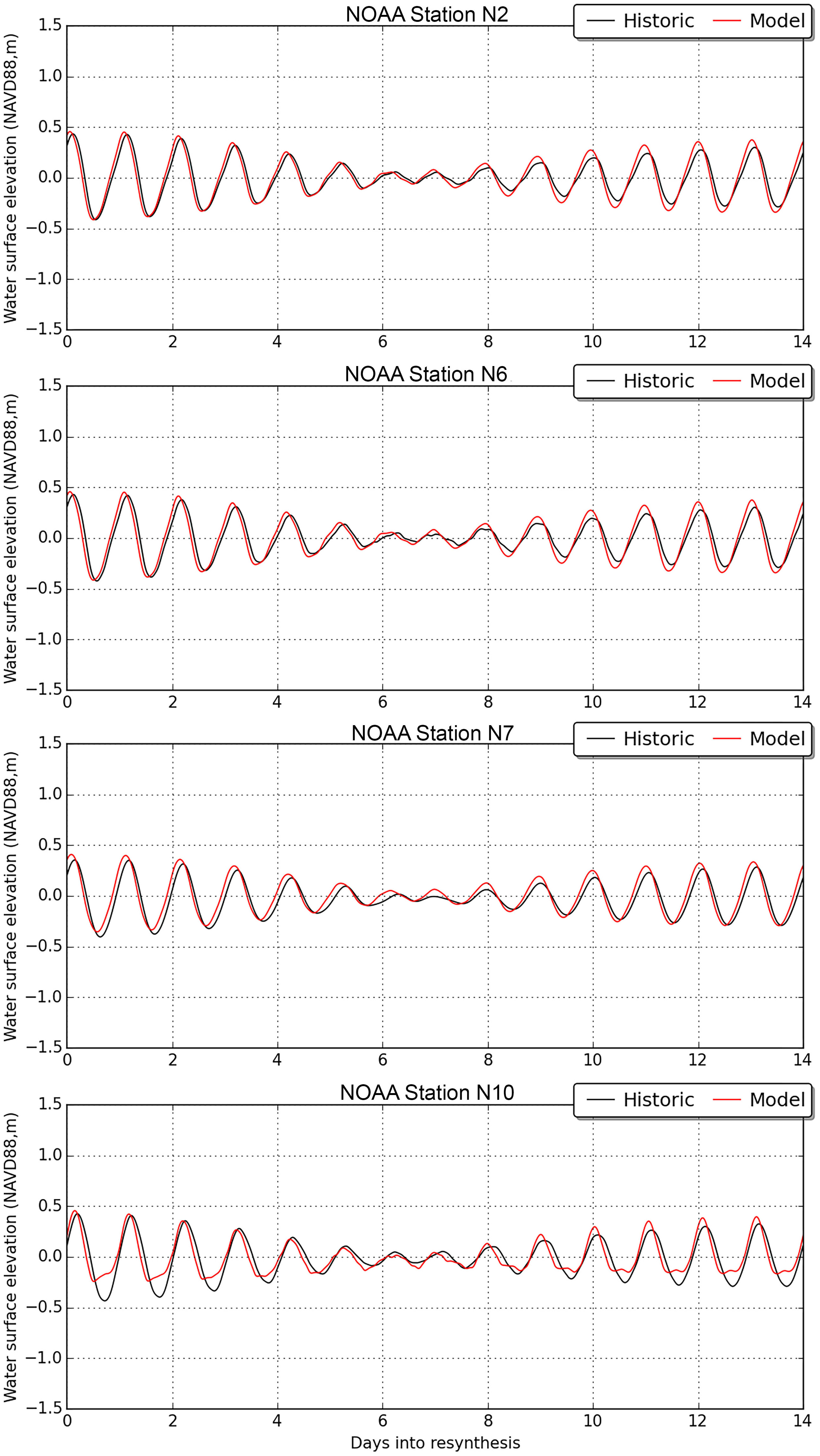
Figure 3 Tidal resynthesis of observed and modeled tidal constituents for the first spring-neap cycle of a tidal epoch (~14.7 days) at four select tide gauge stations (locations in Figure 1).

FIGURE 4

Figure 4 Comparison of the dominant harmonic constituent amplitudes (top) and phases (bottom) measured by NOAA tide gauges and predicted by MSAL model. Difference bands (dashed lines) are located at 0.025 and 0.05 m in the amplitude plot and 10˚ and 20˚ in the phase plot.

To validate the MSAL model with respect to salinity transport, a 101-day salinity simulation was performed for the time period of May 14, 2016 to August 23, 2016, a quiescent period prior to the occurrence of Hurricane Hermine and when salinity observations at the Point aux Chenes water quality station (GNDPCWQ; Figure 1) on the Mississippi side of the estuary were fairly available without gaps in the data. The MSAL-modeled water levels were output every hour at the location of the Dauphin Island tide gauge (NOAA station 8735180/DPAI1 https://tidesandcurrents.noaa.gov/stationhome.html?id=8735180; Figure 1) and compared with observations (Figure 5). Overall, water levels matched well in amplitude and phase. Discrepancies between the modeled and observed water levels can be seen particularly during periods of low water (e.g., around June 9) where the model overpredicted the low water levels. This could be a result of the coarse spatial resolution of the meteorological forcing capturing larger offshore wind patterns rather than localized nearshore wind patterns affecting the study area. However, the RMSE in the water levels was 0.13 m, illustrating that the model performs well at reproducing the wind-driven hydrodynamics during this time period.

FIGURE 5

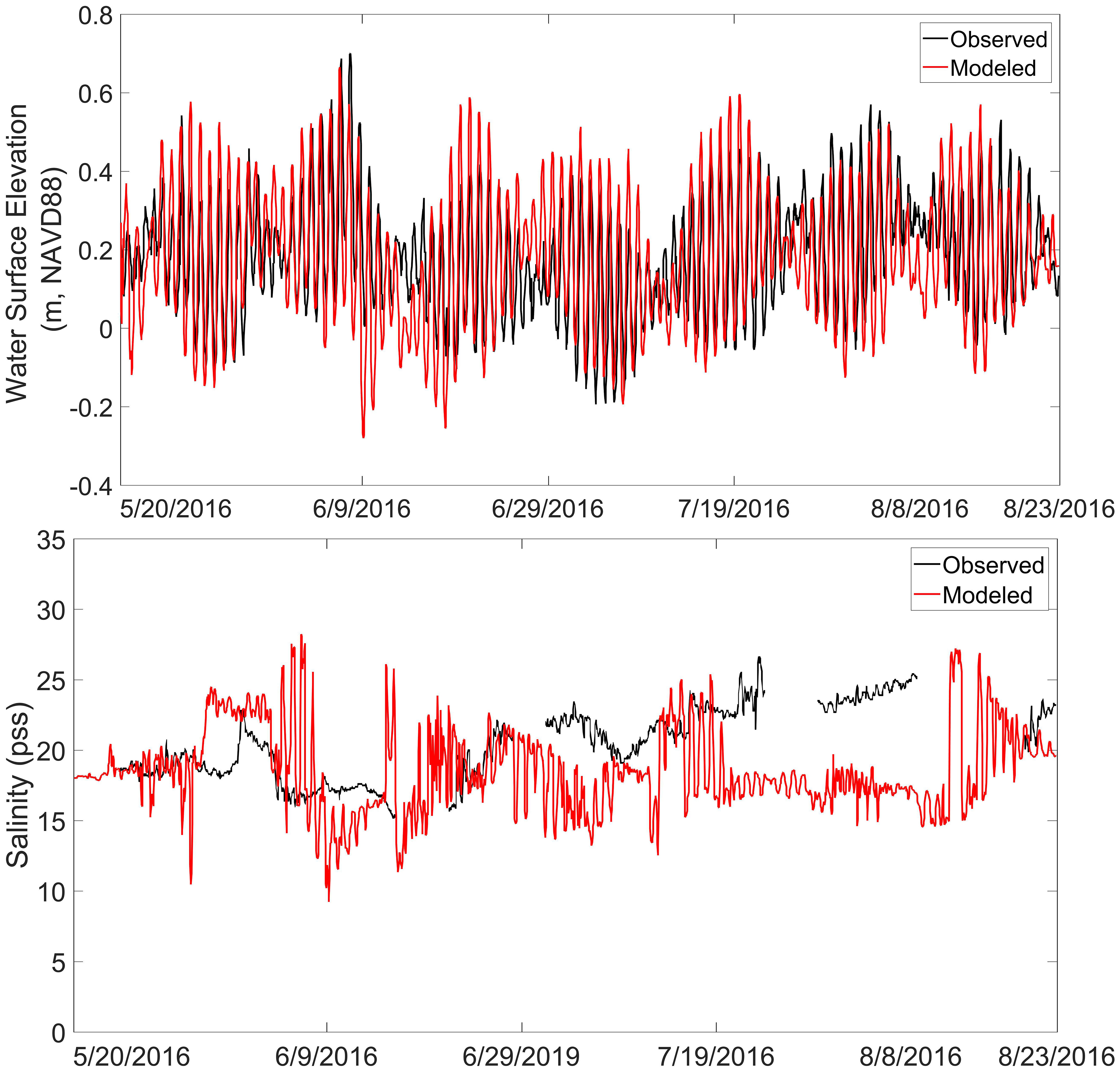
Figure 5 MSAL modeled versus observed water surface elevations at the Dauphin Island tide gauge (top) and salinity concentrations at GNDPCWQ station (bottom).

Modeled hourly salinity concentrations were compared with hourly observations at GNDPCWQ (Figure 5). The model captures the daily variations in salinity corresponding to diurnal tidal flows, as well as periods of decreasing salinity (e.g., from June 8 -18) and increasing salinity (e.g., June 27-29) that result from low- and high- water levels. Overall, the modeled salinity signal has more variability than observations and is generally overpredicted with an RMSE of 4.47 pss. The observed salinity distribution (mean and standard deviation) at GNDPCWQ for the time period was 18.45 ± 1.55 pss, and the modeled salinity distribution was 18.52 ± 2.97 pss. This indicates that the model captures the average salinity trends but shows more variation in daily maximum and minimum salinity than the observations. The errors in salinity are likely attributed to limited spatial salinity data for initial conditions, particularly on the Mississippi side of the estuary where the GNDPCWQ station is located. The influence of freshwater flows due to precipitation may also be responsible for the lower observed salinity. The validation period spans the months with the highest rainfall (rainy season) in Mississippi and Alabama; however, the model is unable to simulate precipitation. Additionally, previous research has shown that DG-SWEM may require 6-9 months of simulation time for the modeled salinity field to achieve dynamic equilibrium and not be sensitive to the initial conditions (Mulamba et al., 2019). Nonetheless, this RMSE is within reasonable error bounds based on previous work (Bacopoulos et al., 2017; Mulamba et al., 2019). Calibration of input parameters to achieve reduced errors was not performed in order to avoid “tuning” the model to a specific time period.

2.5 Simulations of restoration alternatives

The impact of the restoration alternatives was assessed in two parts. A tidal hydrodynamic assessment was conducted to understand the impacts of reconstructing the interior headlands on tidal amplitudes and currents. For this, a 45-day astronomic tide simulation was performed for each alternative. Model output consisted of depth-integrated velocities, amplitudes and phases of harmonic constituents as well as the maximum elevations of water and maximum velocities for the duration of the simulation.

A salinity transport assessment was conducted to determine the impact of the restoration alternatives on spatial salinity patterns. A quiescent frontal and tropical period were simulated to capture the effects of seasonal wind patterns on salinity. Long-term wind data from 2011 – 2019 was obtained at two NOAA National Data Buoy Center (NDBC) stations located in Dauphin Island, AL (DPAI1) and Cedar Point, AL (CRTA1) (see locations in Figure 1). The hourly wind records for each gauge were divided by wind direction and binned by wind speed (Figure 6). Both gauges show similar directional patterns with the predominant wind directions being north/northeast and southeast. Wind speeds were further divided into frontal (November – May) and tropical (June – October) periods to assess seasonal effects on wind speeds and direction (Figure 6). The frontal season is dominated by winds from the north, northeast and southeast. The tropical season has mixed wind directions with southwest being the most dominant, but with the highest wind speeds from the north/northeast and southeast. To develop model forcing for MSAL, the long-term wind data were compared with data for the year 2016 at both NDBC stations; this year was chosen due to the availability of salinity observations used for initial conditions and model validation. The 2016 wind record shows good agreement with the long-term wind patterns in terms of wind direction and wind speed magnitude (Figure 6). Therefore, 2016 was selected as a representative year to simulate the seasonal patterns of winds on salinity. The frontal period was selected from January 1, 2016 – March 27, 2016; this was a quiescent period ahead of a major cold front. The tropical period was selected from June 1, 2016 – August 23, 2016, a quiescent period without tropical cyclone activity (prior to the formation of Hurricane Hermine). Quiescent periods without storms are selected to reduce the influence of drivers such as freshwater flows, precipitation and surface runoff that may affect salinity levels that the model is unable to account for. MSAL was forced with the NGOM-RT water levels and the NAM meteorological forcing for each season. Model output from MSAL consisted of depth-integrated salinity concentrations and water levels.

FIGURE 6

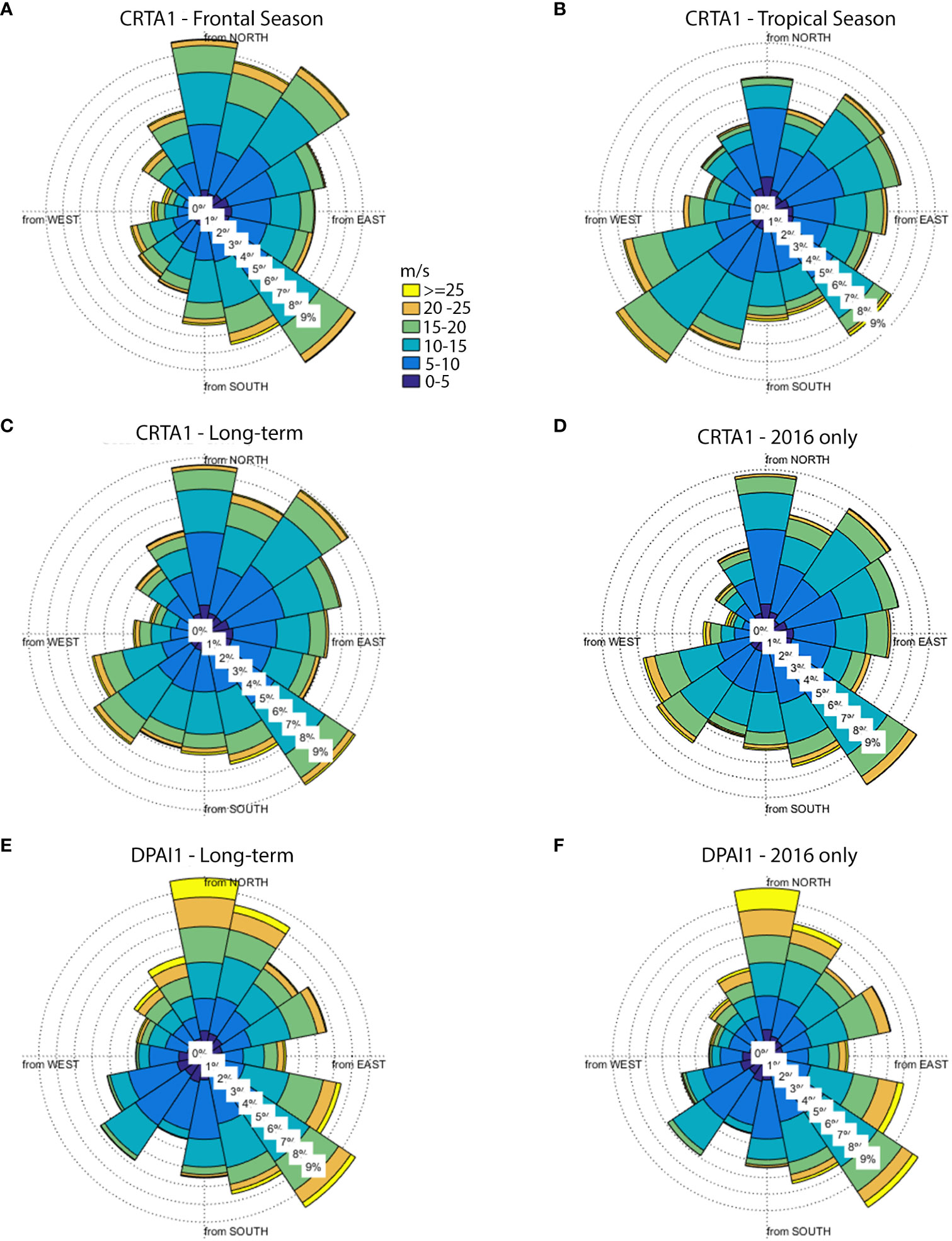
Figure 6 Wind roses for Cedar Point, AL: (A) Frontal season, (B) Tropical season, (C) long-term and (D) 2016 only; and for Dauphin Island, AL: (E) long-term and (F) 2016 only.

For both the tidal hydrodynamic and salinity assessments, a SLR of 0.5 m was also considered to assess the impacts of SLR on estuarine hydrodynamics and salinity with and without the restoration alternatives. This amount of SLR corresponds to a high projection of SLR by the year 2050 (Sweet et al., 2022). The incorporation of a SLR assessment is not meant to forecast a future estuary state, but rather to understand how the proposed restoration alternatives behave under a plausible future SLR in the lifetime of the project. In total, 6 tidal hydrodynamic simulations were performed: three restoration alternatives (no-action, GBI and All Alternatives) that were modeled under two sea level conditions (present-day and 0.5 m of SLR). Additionally, 12 salinity simulations were performed: three restoration alternatives (no-action, GBI and All Alternatives) that were modeled under two seasons (frontal and tropical) and two sea level conditions (present-day and 0.5 m of SLR).

3 Results

3.1 Tidal hydrodynamic assessment of alternatives

Within the Grand Bay estuary, the modeled tidal amplitude (i.e., the amplitude of the tide with respect to mean sea level) is on the order of 44 cm. For both the GBI and All Alternatives scenarios, the restoration actions do not alter tidal amplitudes within the estuary; this is also the case for the scenarios with 0.5 m of SLR. Figure 7 shows the maximum tidal velocities for the no-action scenario and the change in maximum tidal velocities with the restoration alternatives for present-day conditions (panels a-c) and with 0.5 m of SLR (panels d-f). In the GBI scenario, tidal velocities decrease by approximately 5 cm/s (50% decrease from the no-action scenario) in the areas immediately behind GBI but increase by approximately 5-10 cm/s (50-100% increase from the no-action scenario) in the eastern bay. Similar patterns are seen in the All Alternatives scenario, with small decreases in the area immediate to Isle aux Dames. This indicates that the GBI restoration alternative is more influential in changing the tidal hydrodynamics of the estuary than Marsh Island and Isle aux Dames, likely due to its size and position within the embayment. Residual currents (the net tidal current throughout the duration of the simulation) indicate changes in the direction of currents with the alternatives present (Figures 8A–C). With the GBI alternative, currents diffract around the restored island and are directed more westward behind the island; this creates a counterclockwise residual eddy (rotary current) at the tip of the island. In the All Alternatives scenario, there are localized directional changes in the residual currents around Isle aux Dames and Marsh Island as currents diffract, but otherwise the currents remain relatively the same as the in the no-action scenario.

FIGURE 7

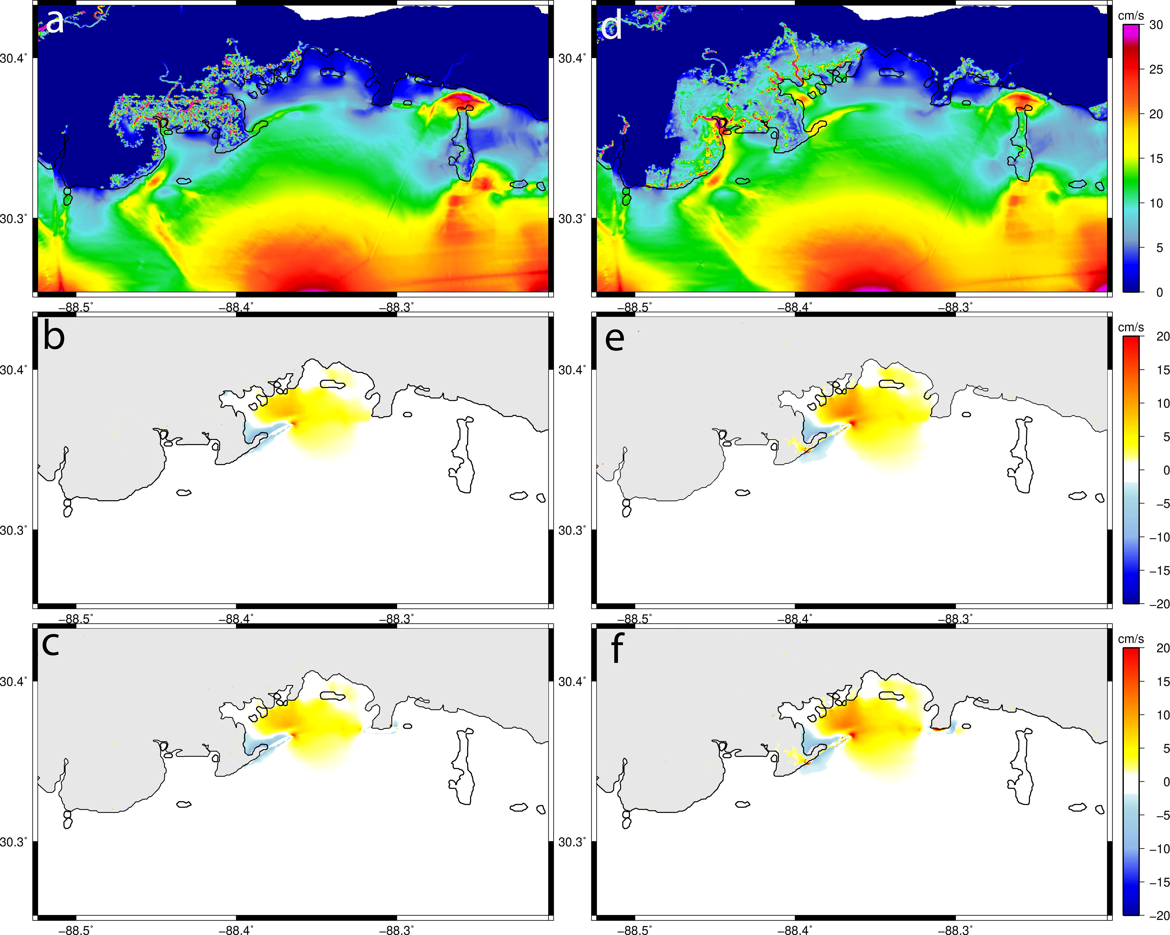
Figure 7 Maximum tidal velocities (cm/s) for the (A) no-action and (D) no-action with 0.5 m of SLR scenarios; and the change in maximum tidal velocities (cm/s) for (B) the GBI scenario and (E) the GBI with 0.5 m of SLR scenario, (C) All Alternatives scenario and (F) All Alternatives with 0.5 m of SLR scenario. For (B–F), warmer colors indicate increases in maximum tidal velocities with the alternative, cooler colors indicate decreases in maximum tidal velocities with the alternative.

FIGURE 8

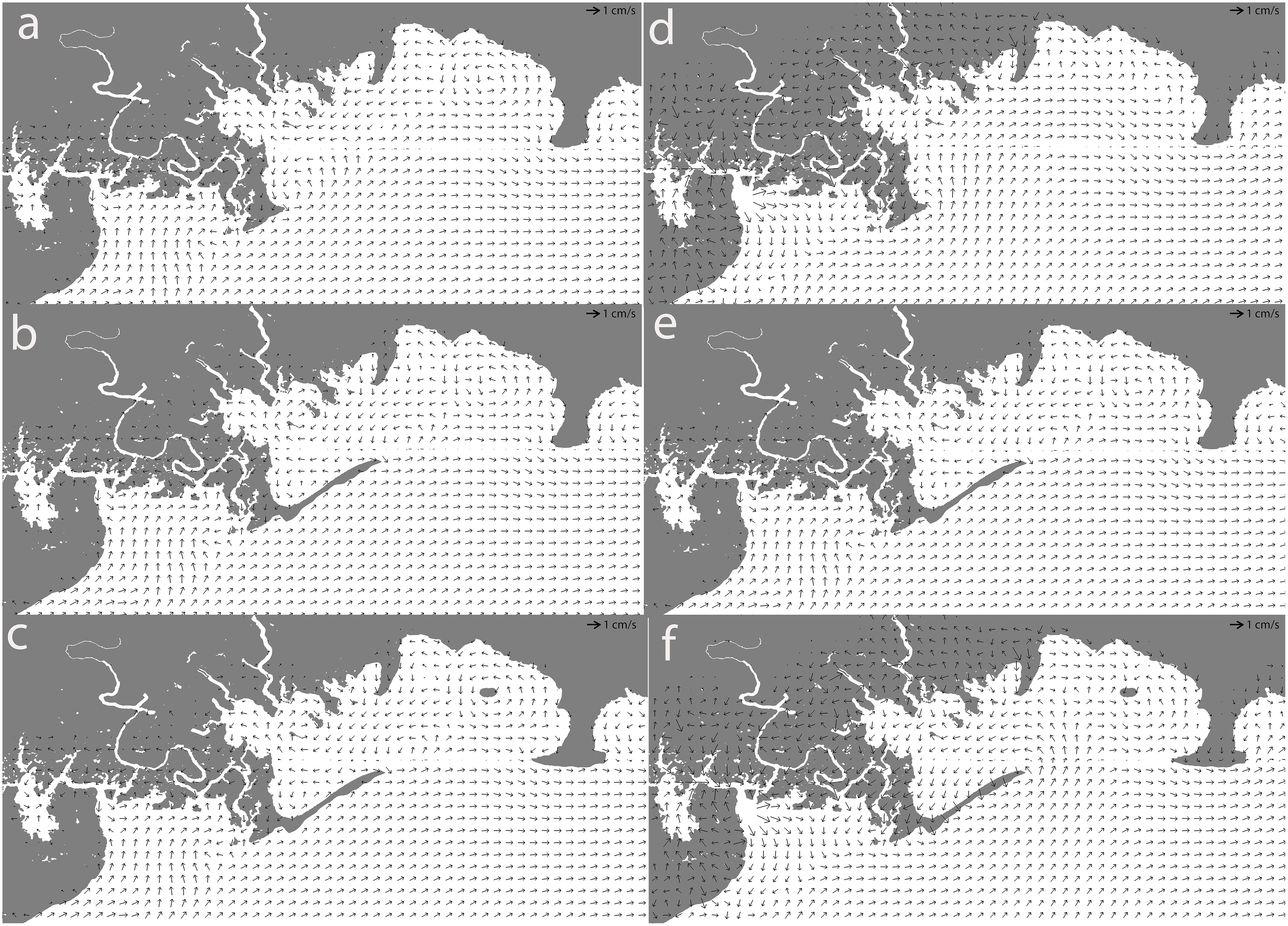
Figure 8 Tidal residual velocities (cm/s) for the (A) no action scenario, (B) GBI scenario and (C) All Alternatives (D) no-action with 0.5m SLR, (E) GBI with 0.5 m of SLR and (F) All Alternatives with 0.5 m of SLR scenarios. Black errors represent the residual velocity magnitude (1 cm/s) and direction.

For the no-action scenario with 0.5 m of SLR, the maximum tidal velocities increase by ~5-7 cm/s within the marsh, tidal creeks and embayments compared to the present-day scenario. The same patterns of increases and decreases in the maximum tidal velocities exist in the GBI and All Alternatives scenarios with 0.5 m of SLR as the present-day scenarios. With 0.5 m of SLR, residual currents are directed more northeastward and southward than in the present-day no-action scenario (Figures 8D–F). With the GBI alternative, currents move westward alongshore of the island with a rotary current at the tip of GBI that is larger in diameter than the present-day scenarios. In the All Alternatives scenario, residual currents again diffract around Marsh Island and Isle aux Dames.

3.2 Salinity assessment of alternatives

To observe salinity changes in the estuary with and without the restoration alternatives, the average salinity concentration at each node in the model mesh over the duration of the simulation was calculated from the spatial time-series output for each scenario (Figures 9, 10). Additionally, time-series of salinity concentrations (pss) were output every hour at four locations that were selected based on their proximity to the restoration alternatives (Stations 1 and 2 in Figure 1) and nearby oyster leases (see Stations 3 and 4 in Figure 1). Cumulative distribution functions (CDFs) of salinity at each station were developed to assess changes in the salinity distribution for each simulation (Figures 11, 12). The mean salinity concentrations were calculated from the CDFs at each station as well as at the GNDPCWQ station on the Mississippi side of the estuary for comparison (Table 1). The CDFs show changes in mean salinity, as well as the extremes (maximum and minimum), which are meaningful in terms of ecosystem health and may not be represented if salinity is generalized as a mean (Yurek et al., 2023).

FIGURE 9

Figure 9 Average salinity for the frontal period (A) no-action scenario. Difference in average salinity for the frontal period between the (B) GBI alternative and no-action and (C) All Alternatives and no-action. Average salinity for the frontal period with 0.5 m of SLR (D) no-action scenario. Difference in average salinity for the frontal period with 0.5 m of SLR between the (E) GBI alternative and no-action and (F) All Alternatives and no-action. For the difference plots, warmer colors indicate increases in the average salinity with the alternative, cooler colors indicate decreases in the average salinity with the alternative.

FIGURE 10

Figure 10 Average salinity for the tropical period (A) no-action scenario. Difference in average salinity for the tropical period between the (B) GBI alternative and no-action and (C) All Alternatives and no-action. Average salinity for the tropical period with 0.5 m of SLR (D) no-action scenario. Difference in average salinity for the tropical period with 0.5 m of SLR between the (E) GBI alternative and no-action and (F) All Alternatives and no-action. For the difference plots, warmer colors indicate increases in the average salinity with the alternative, cooler colors indicate decreases in the average salinity with the alternative.

FIGURE 11

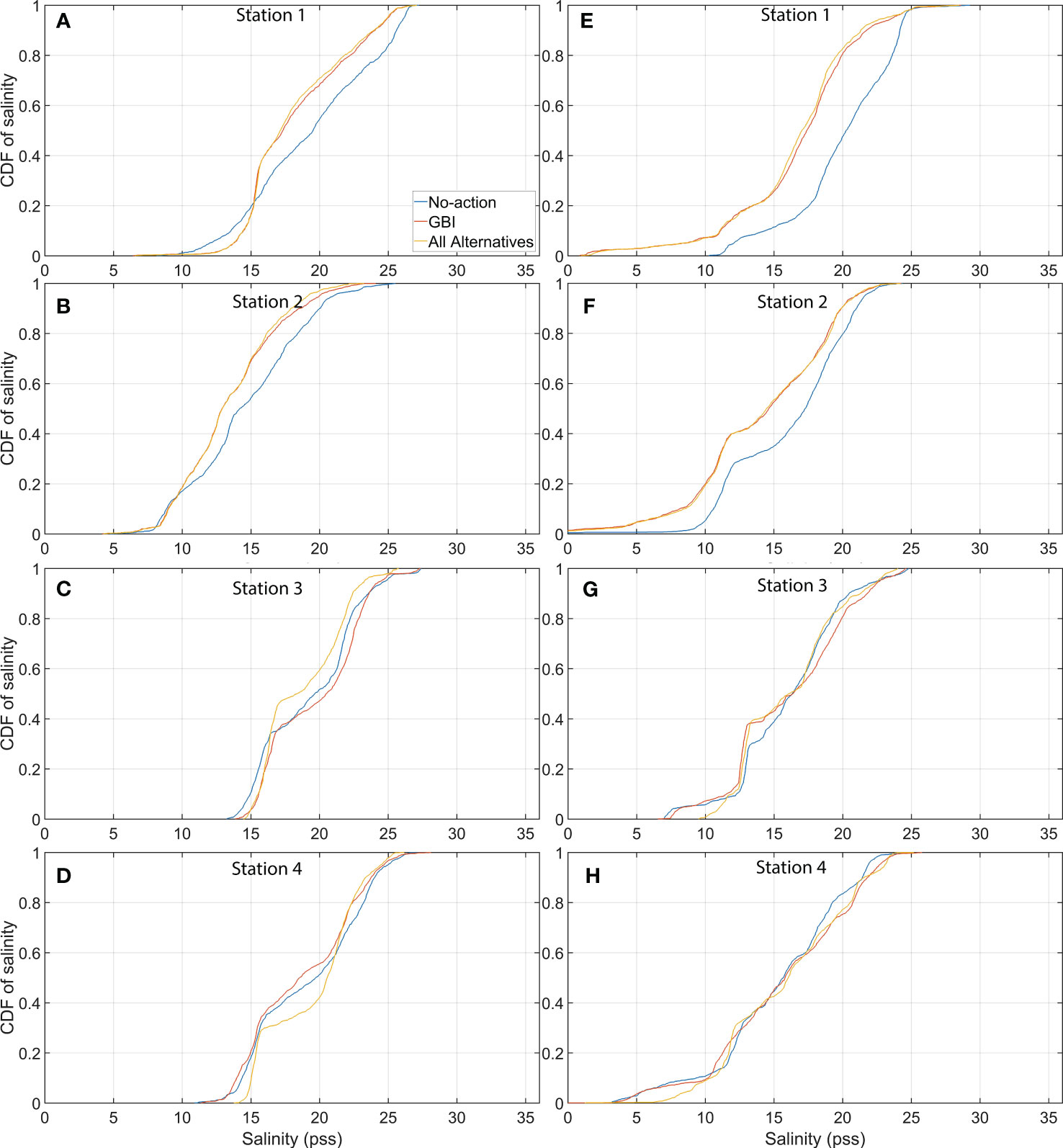
Figure 11 Cumulative distribution function (CDF) plots of salinity at Stations 1-4 (see locations in Figure 1) for the Frontal simulation (A–D) and the Frontal with 0.5 m of SLR simulation (E–H).

FIGURE 12

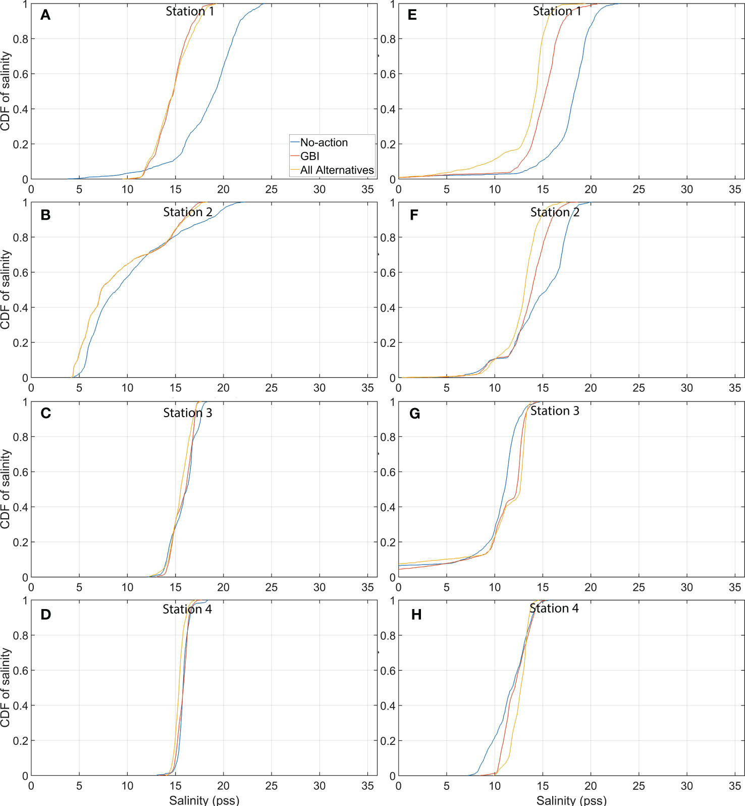
Figure 12 Cumulative distribution function (CDF) plots of salinity at Stations 1-4 (see locations in Figure 1) for the Tropical period simulation (A–D) and the Tropical with 0.5 m of SLR simulation (E–H).

TABLE 1

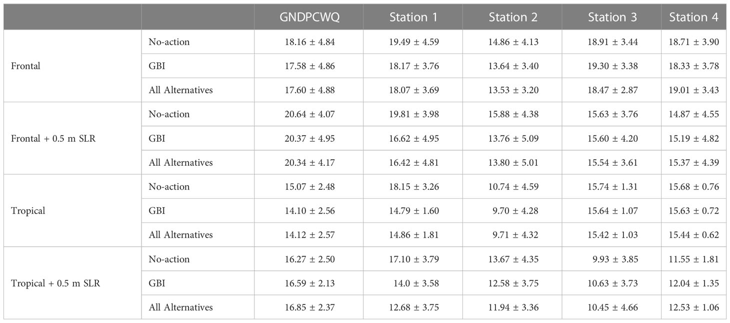
Table 1 Mean ± standard deviation of salinity (pss) for each restoration scenario at output stations.

3.2.1 Frontal period

The spatial plots of average salinity concentrations for the no-action frontal period show that salinity ranges from 25 – 30 pss in the Mississippi Sound, and between 15 and 20 pss within Grand Bay (Figures 9A–C). The changes in average salinity concentrations with the GBI alternative are low in magnitude (on the order of ±2 pss). Salinity increases in the areas immediate to GBI and decreases further landward and seaward of the island. In the All Alternatives scenario, there are additional areas in close proximity to the Marsh Island and Isle aux Dames that have decreased salinity by 1-2 pss.

The CDFs at the four stations (Figures 11A–D) have similar salinity distributions for the no-action scenario with 80% of salinity values less than 25 pss at Station 1, 80% of values less than 23 pss at Station 3 and 80% of values less than 24 pss at Station 4. Station 2 was least saline with 80% of salinity values less than 18 pss. The GBI alternative has more of an influence on the salinity distribution at Stations 1 and 2 than 3 and 4. There is a small shift to a lower salinity distribution at Station 1 (80% of values less than 23 pss when GBI is present; mean ± SD decreases from 19.49 ± 4.59 in the no-action scenario to 18.17 ± 3.76) and Station 2 (80% of values less than 16 pss when GBI is present; mean ± SD decrease from 14.86 ± 4.13 to 13.64 ± 3.40.). At Stations 3 and 4, there are minimal changes in the CDFs. In the All Alternatives scenario, the additional features have more of an influence at Stations 3 and 4 than at Stations 1 and 2 due to proximity; the CDFs of salinity are almost identical as in the GBI scenario at Stations 1 and 2, and there are minimal changes in the mean ± SD of salinity. At Station 3, there is a small decrease in the middle of the salinity distribution in the All Alternatives scenario from the no-action scenario; in the no-action scenario, 50% of the values are less than 18 pss compared to 55% of values less than 18 pss in the All Alternatives scenario. However, the mean ± SD of salinity stays relatively the same in both scenarios. At Station 4, there is also a shift in the middle of the distribution, with 50% of values less than 17 pss in the no-action scenario increasing to 50% of values less than 20 pss in the All alternatives scenario. There is minimal shift in the mean ± SD from 18.71 ± 3.90 to 19.01 ± 3.43 pss.

3.2.2 Frontal period with 0.5 m of SLR

The spatial plots of average salinity for the frontal period with 0.5 m of SLR show similar salinity values as the present-day scenarios, but have lower salinity values (on the order of 15 pss) along the estuarine shoreline (Figures 9D–F). The GBI alternative generally reduces the average salinity by approximately 2 to 3 pss in the areas seaward of the island. Small increases in salinity (1 pss) are seen in the embayments east of the estuary. Changes in the average salinity for the All Alternatives scenario are similar to those seen in GBI, with some additional decreases near Isle aux Dames and Marsh Island.

The frontal period with 0.5 m of SLR scenarios show similar behavior in the CDFs at the four stations as in the present-day scenarios (Figures 11E–H). In the no-action scenario with 0.5 m of SLR, salinity is slightly higher than present-day at Stations 1 and 2 with 80% of salinity values less than 24 pss and 80% of values less than 20 pss, respectively. Stations 3 and 4 show decreases in salinity from present-day conditions, with 80% of values less than 19 pss at both stations. The GBI alternative again is more influential at changing the salinity distribution at Stations 1 and 2 due to proximity, with 80% of values less than 20 pss at Station 1, and 80% of values less than 18 pss at Station 2; the mean ± SD decreases from 19.81 ± 3.98 in the no-action scenario to 16.62 ± 4.95 at Station 1 and 15.88 ± 4.38 to 13.76 ± 5.09 at Station 2. At Stations 3 and 4, there are minimal changes in the CDFs. In the All Alternatives scenario, the CDFs are almost identical as the GBI scenario at Stations 1 and 2. At Stations 3 and 4, there are minimal changes in the CDFs between the no-action, GBI and All Alternative scenarios, indicating that under SLR, the Marsh Island and Isle aux Dames scenarios are even less influential on salinity patterns at these locations.

3.2.3 Tropical period

For the tropical period, average salinity concentrations in the estuary are lower than during the frontal period as a result of predominant southwest winds and reduced fetch (Figures 10A–C). Changes in the average salinity between the no-action and GBI scenarios indicate mostly decreases (between 1 and 3 pss) surrounding the restored island, with small increases (~1 pss) in the embayments to the east. There are small (~ 1 pss) changes to salinity on the Mississippi side of the estuary near the shoreline. The All Alternatives scenario shows similar order of magnitude of changes as in the GBI scenario with decreases surrounding GBI and around Marsh Island and Isle aux Dames.

Similar to the frontal period, the CDFs (Figures 12A–D; Table 1) show that Station 1 has the most saline conditions with 80% of values less than 21 pss and a mean ± SD of 18.15 ± 3.26 pss, whereas Station 2 has the least saline conditions with 80% of values less than 16 pss and mean ± SD of 10.74 ± 4.59 pss. As seen in the frontal period, GBI is most influential in altering the salinity distribution at Stations 1 and 2 given their proximity to the restored island. At both stations, GBI results in a lower salinity distribution with 80% of values less than 16 pss at Station 1 and 80% of values less than 14 pss at Station 2. The mean ± SD also decrease to 14.79 ± 1.60 pss at Station 1 and 9.70 ± 4.28 at Station 2 from the no-action scenario. Decreases in the standard deviation indicate there is less spread in the salinity distribution, as seen in the CDFs. At Stations 3 and 4, there are minimal changes (less than 1%) in the CDFs of salinity with GBI present. For the All Alternatives scenario, there are minimal changes in the CDFs of salinity from the GBI scenario at Stations 1 and 2, indicating that Marsh Island and Isle aux Dames are not influential in salinity patterns in this part of the estuary. At Stations 3 and 4, there are minimal changes in the CDFs of salinity from the no-action scenario, further supporting that Marsh Island and Isle aux Dames have little impact on salinity when wind directions are predominantly from the southwest.

3.2.4 Tropical period with 0.5 m of SLR

For the tropical period with 0.5 m of SLR, average salinity values followed similar patterns as the present-day scenario, but again were lower by ~5 pss along the eastern estuarine shoreline (Figures 10D–F). Changes in the average salinity between the restoration alternatives follow similar patterns as the present-day scenarios; there are decreases in salinity (on the order of 2 to 4 pss) surrounding GBI, with small increases (1 pss) in the eastern estuary. Overall, the changes in average salinity for the tropical period indicate that the impact of the restoration actions on salinity values is rather minimal (less than 4 pss) and localized in the vicinity of the restored features.

The CDFs (Figures 12E–H) show that out of the four stations, Station 1 has the most saline conditions with 80% of salinity values less than 19 pss and a mean ± SD of 17.10 ± 3.79 for the no-action scenario. Station 3 is the least saline with 80% of salinity values less than 13 pss and a mean ± SD of 9.93 ± 3.85 pss. The GBI alternative is again most impactful at Station 1 due to its proximity to the restored island, which results in a shift to a lower salinity distribution (80% of values less than 16 pss) and a decrease in the mean ± SD to 14.0 ± 3.58 pss (18% decrease in mean). A shift to a lower salinity distribution is also seen at Station 2 with 80% of values less than 15 pss and an 8% decrease in the mean. Stations 3 and 4 have small shifts to higher salinity distributions (7% and 4% increases in the mean at Stations 3 and 4, respectively), indicating the GBI has more of an impact on the salinity dynamics in the eastern estuary under SLR. The All Alternatives scenario further lowers the salinity distribution at Station 1 (80% of values less than 15 pss; 26% decrease in the mean) and Station 2 (80% of values less than 14 pss; 13% decrease in the mean) from the no-action scenario. Stations 3 and 4 show minimal changes in the salinity distributions from the GBI scenario (less than 3%), further indicating that the restored Marsh Island and Isle aux Dames in the All Alternatives scenario have little impact on salinity during the tropical period.

4 Discussion

4.1 Influence of large-scale restoration features

In the context of previous studies, most assessments of restoration actions on salinity have been observations from post-construction monitoring (e.g., U.S. Army Corps of Engineers Mobile District (2016) and Byrnes et al. (2018)). More recently, predictive numerical models have been used to assess the impacts of potential restoration actions on estuarine hydrodynamics and salinity prior to construction. This has included assessing potential river diversions (Ou et al., 2020), barrier island sand placement strategies (Enwright et al., 2020) and water resource management (Qiu and Wan, 2013). Models have shown that closing storm-induced barrier island breaches can lower salinity in back-bay areas (e.g., Katrina Cut at Dauphin Island, AL (Park et al., 2014) and Camille Cut at Ship Island, MS (U.S. Army Corps of Engineers Mobile District, 2016)). However, the impacts of creating new islands and headlands which significantly change the geometry of the shoreline and resulting fetch in estuaries has not been well studied. This research improves the overall understanding of the influence of large-scale restoration features on the physical processes (tidal hydrodynamics and salinity) in an open coast, marine dominant estuary. Out of the three restoration alternatives, GBI had the largest footprint and substantially altered the geometry of the shoreline and fetch within the bay. As a result, it had the greatest influence on hydrodynamic and salinity patterns. For both the frontal and tropical periods, GBI sheltered the western bay and generally reduced salinity in the areas immediately behind the restored island. It had minimal influence in the eastern estuary, on the Mississippi side of the estuary and offshore. In comparison, Marsh Island and Isle aux Dames had a small footprint and had small localized influences on salinity in the immediate areas to the alternatives. The largest changes occurred for the Frontal period when winds are predominately southeast and north/northeast and Isle aux Dames reduced the fetch to the eastern bay (stations 3, 4). This illustrates that interior headland restoration has localized effects on the physical processes within the vicinity of the features.

From a biological standpoint, changes in current velocities and salinity ranges could affect the ecosystems within the estuary. The relative differences in the modeled salinity between the restoration alternatives were on the order of ±5 pss. Some of these changes were observed in the vicinity of existing oyster leases within the estuary (near Stations 3, 4). Previous research has shown that the eastern oyster, commonly found in estuaries in the northern Gulf of Mexico, can tolerate salinities ranging from 0 to 42 pss, with optimal growth occurring between 14-29 pss (Shumway, 1996). These oysters are sensitive to extreme salinities (<5 and >35 pss), particularly if they are exposed for prolonged periods of time (Marshall et al., 2021a; Marshall et al., 2021b). Oysters can be impacted at both extremes in locations where salinity broadly fluctuates, which may affect feeding rates, respiration and even result in mortality (Yurek et al., 2023). The mean salinity for all scenarios in the frontal and tropical periods remained within the optimal range. The salinity distributions did not exceed the upper tolerance of 35 pss in any of the scenarios; however, the model was not initialized with salinity values greater than 36 pss, which could occur due to processes such as evaporation that the model is unable to capture. The CDFs (Figures 11, 12) at the stations generally indicated shifts towards lower salinity regimes with the restoration alternatives; there were a few exceptions at Stations 3 and 4 in the All Alternatives scenario and the scenarios with SLR, where the middle of the distribution was slightly higher, thus potentially squeezing suitable salinity range for oyster growth and recruitment. In terms of low salinity, the CDFs show that for the frontal simulations (Figures 11A–D; Table 2), salinity did not decrease beneath 5 pss at any of the stations for any of the restoration alternatives. For the frontal simulations with 0.5 m of SLR (Figures 11E–H; Table 2), Station 2 and Station 4 experienced low salinity with 1% of values less than 5 pss and 3% of values less than 5 pss in the no-action scenarios, respectively. The GBI alternative increased low salinity exposure at Station 1 to 3% of values less than 5 pss and Station 2 to 5% of values less than 5 pss; low salinity exposure remained the same at Station 4. The All Alternatives scenario did not further alter low salinity exposure at Station 1 or 2, but decreased low salinity exposure at Station 4 to 0% of values less than 5 pss. For the tropical simulations (Figures 12A–D; Table 2), Station 2 was the only station impacted by low salinity, with 2% of values less than 5 pss in the no-action scenario. This increased to 14% of values less than 5 pss in both the GBI and All Alternatives scenarios. In the no-action tropical scenarios with 0.5 m of SLR (Figures 12E–H, Stations 1, 2 and 3 experienced low salinity with 2% of values less than 5 pss, 1% of values less than 5 pss and 7% of values less than 5 pss, respectively; Station 4 did not experience low salinity. The GBI alternative did not further alter exposure to low salinity ranges; however, the All Alternatives scenario increased low salinity exposure to 3% of values less than 5 pss at Station 1 and 10% of values less than 5 pss at Station 3; Station 2 and Station 4 remained the same as the no-action scenario. These results show that overall, SLR was more impactful to low salinity exposure in terms of duration and spatiality than the presence of the restoration alternatives; this is similar to the findings of previous work (Wang et al., 2020). The model results support the need for a more detailed habitat suitability study to determine if these changes in salinity could be impactful to oysters or other species such as submerged aquatic vegetation (SAV).

TABLE 2

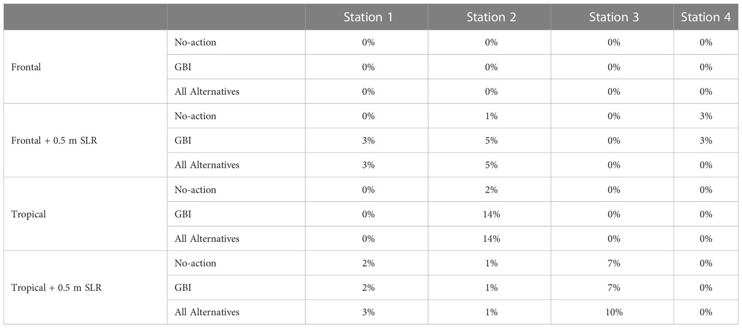
Table 2 Percent change in the daily maximum, daily mean and daily minimum salinity calculated over the combined frontal and tropical periods for the no-action and no-action with SLR scenarios.

The model results also showed changes in tidal velocities and residual currents. Current velocities are critical to oyster larval transport and settlement, nutrient availability, oyster filtration and growth and mortality (Harsh and Luckenbach, 1999; Smith et al., 2009; Campbell and Hall, 2019; Theuerkauf et al., 2019; La Peyre et al., 2021; Lipcius et al., 2021; Salatin et al., 2022). Current velocities below 15 cm/s have been found optimal for required nutrient delivery and oyster filtration (Theuerkauf et al., 2019); maximum currents are below this threshold for the majority of the study area with the restoration alternatives. In terms of salt marsh productivity, flood dominant currents typically increase suspended sediment concentrations at the marsh boundary, which supplies more marine sediment to the marsh. Ebb dominant currents can reduce sediment supply to the marsh and move sediment offshore (Friedrichs and Perry, 2001). A follow on to this study uses a process-based sediment transport model to assess if these restoration alternatives would affect suspended sediment concentrations and sediment fluxes in the estuary and to the marsh (see companion paper Jenkins et al., 2023 Frontiers in Marine Science in review).

4.2 Limitations in modeling

All modeled changes in salinity were on the order of ±5 pss, which is within the error of the model. However, this analysis is meant to look at the relative changes in salinity between scenarios, rather than the values themselves. Further, there is high confidence in the hydrodynamics based on the validation, which showed changes in velocities and residual currents with the restoration alternatives; these results support the simulated changes in salinity concentrations. There are limitations in this study including the availability of spatial and temporal salinity data to initialize the model. This study relied on CTD casts that were collected over a 4-day period in May 2016 at a limited number of locations within Grand Bay; there was no other spatial or temporal data available within the estuary to parameterize initial salinity conditions. Therefore, there is uncertainty in the spatial values of salinity concentrations particularly in the areas outside of the CTD casts (e.g., on the Mississippi side of the estuary where the GNDPCWQ station is, which was used for validation). Further, because these data were collected in May, the values of salinity concentrations may vary during the frontal and tropical seasons from the modeled conditions. However, the relative differences in salinity between scenarios would likely stay the same. As mentioned in Section 2.5, the incorporation of SLR was not meant to forecast the state of the estuary in the future, but rather to isolate the behavior of the proposed alternatives under a plausible future SLR in the lifetime of the project. Integrated modeling approaches that consider the feedbacks between hydrodynamics and morphology under SLR can provide a more holistic understanding of potential future estuarine conditions (Passeri et al., 2015).

4.3 Effects of sea level rise on salinity

The response of salinity to SLR varied, resulting in increases and decreases in the salinity distributions from the present-day scenario. Comparing the average salinity for the frontal and tropical no-action scenarios (Figures 9, 10) shows there were increases in the average salinity under SLR in the middle of the bays, but reductions in the average salinity closer to the estuarine shoreline, particularly along the eastern side of the estuary. This is also seen in the CDFs of the salinity distributions where the salinity distribution increased at Station 1 and Station 2 but decreased at Stations 3 and 4. To further illustrate the nonlinear response, the daily maximum, mean and minimum salinity values were calculated for the no-action and no-action with 0.5m of SLR across the frontal and tropical periods; the frontal and tropical periods were combined to determine the daily salinity values independent of seasonal effects. Values were calculated at the 4 stations as well as at GNDPCWQ and DPAI1. Table 3 shows the percent change in the daily maximum, mean and salinity between the present-day scenario and the 0.5 m of SLR scenario. Out of all of the stations, DPAI1 had the lowest percent change (ranging from -0.6 to -1.4%) in the daily maximum, mean and minimum salinity under SLR, illustrating a more static response (i.e., no change) in salinity offshore. Changes in salinity increased with distance into the estuary (e.g., Station 1 versus Station 2). At all stations, SLR caused larger changes in lower salinity values (i.e., daily minimum) than higher salinity values (i.e., daily maximum). The nonlinear response of salinity with SLR is likely a result of the changing velocities. As the residual velocities in the estuary changed magnitude and direction under SLR, particularly along the estuarine shorelines, there were resulting changes to salinity transport. This is in agreement with previous research that has shown salinity changes were nonlinear with SLR as a result of changes in the current velocities (Moore et al., 2019).

TABLE 3

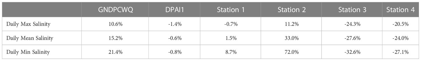
Table 3 Percent change in the daily maximum, daily mean and daily minimum salinity calculated over the combined frontal and tropical periods for the no-action and no-action with SLR scenarios.

5 Conclusions

A two-dimensional DG-SWEM hydrodynamic and salinity model was developed to simulate changes in tidal hydrodynamics and salinity patterns with and without interior headland restoration, for present-day and a future SLR of 0.5 m in the Grand Bay estuary. The model was initialized with observed and modeled salinity measurements and validated for astronomic tides and salinity concentrations. A tidal hydrodynamic assessment indicated the restoration alternatives had no impact on tidal range within the estuary, but changed maximum tidal velocities by ±5 cm/s and changed the directions of residual currents in the areas surrounding the alternatives. Under SLR, similar patterns were observed with slightly larger changes in maximum tidal velocities ( ± 7 cm/s) and additional directional changes in residual currents.

Salinity was modeled for frontal and tropical seasons, with and without SLR. With the restoration alternatives, changes in the average salinity concentrations ranged from ±2 pss for both periods; these changes were confined within bays and had minimal impacts to offshore regions or on the Mississippi side of the estuary. Changes in salinity with the alternatives were greater for the tropical season than the frontal season due to predominant southwest winds and the associated reduced fetch, particularly in the areas behind GBI. The alternatives also changed the salinity distributions at various locations throughout the estuary. Although no areas were exposed to high salinity (>35 pss), some locations experienced small shifts towards higher salinity ranges in the All Alternatives scenario. SLR was more impactful for increasing exposure to low salinity values (< 5 pss) than the restoration alternatives. Both the tidal hydrodynamic and salinity assessments indicated that the GBI alternative was more influential in changing hydrodynamics and salinity than Marsh Island and Isle aux Dames as a result of its size and position in changing the geometry of the shoreline and fetch within the bay. Overall, the modeled results indicate that these large-scale restoration actions have limited and localized impacts on the hydrodynamics and salinity patterns in this open coast estuary. The results also demonstrated the nonlinear response of salinity to SLR, with increases and decreases in the maximum, mean and minimum daily salinity concentrations from present-day conditions. Locations that were more sheltered within the estuary had a more nonlinear response than locations offshore. This nonlinear response was a result of changes in the directions of the residual currents, which affected salinity transport. Overall, this study improves the understanding of large-scale restoration actions on estuarine hydrodynamics and salinity for present-day and future conditions.

Data availability statement

The model inputs and outputs for this study can be found in Passeri et al., 2023 “Modeling the effects of large-scale interior headland restoration on tidal hydrodynamics and salinity transport in an open coast, marine-dominant estuary: Model Inputs and Outputs” U.S. Geological Survey Data Release: https://doi.org/10.5066/P9OO9N0O.

Author contributions

DP developed and applied the numerical model used in this study with advisement from PB and MB. MB provided the numerical model used for boundary conditions. RJ and AP generated the model inputs and boundary conditions. All authors contributed to the paper by reviewing and approving the text. All authors contributed to the article and approved the submitted version.

Funding

This work was funded in part by The Gulf Coast Ecosystem Restoration Council (RESTORE), NOAA’s National Centers for Coastal Ocean Science Competitive Research Program and Research under award NA20NOS4780193, and the USGS Coastal and Marine Hazards and Resources Program.

Acknowledgments

This paper is a result of the research done in collaboration with Alabama Department of Conservation of Natural Resources and Volkert, Inc. The authors would like to thank Dr. Hongqing Wang and the reviewers for their input on this manuscript.

Conflict of interest

The authors declare that the research was conducted in the absence of any commercial or financial relationships that could be construed as a potential conflict of interest.

Volkert, Inc designed the restoration alternatives used in the study in collaboration with the Alabama Department of Conservation of Natural Resources. Any use of trade, firm, or product names is for descriptive purposes only and does not imply endorsement by the U.S. Government.

Publisher’s note

All claims expressed in this article are solely those of the authors and do not necessarily represent those of their affiliated organizations, or those of the publisher, the editors and the reviewers. Any product that may be evaluated in this article, or claim that may be made by its manufacturer, is not guaranteed or endorsed by the publisher.

References

Abelson A., Reed D. C., Edgar G. J., Smith C. S., Kendrick G. A., Orth R. J., et al. (2020). Challenges for restoration of coastsal marine ecosystems in the anthropocene. Front. Mar. Sci. 7. doi: 10.3389/fmars.2020.544105

CrossRef Full Text | Google Scholar

Alizad K., Hagen S. C., Medeiros S. C., Bilskie M. V., Morris J. T., Balthis L., et al. (2018). Dynamic responses and implications to coastal wetlands and the surrounding regions under sea level rise. PloS One 13 (12). doi: 10.1371/journal.pone.0210134

PubMed Abstract | CrossRef Full Text | Google Scholar

Alizad K., Hagen S. C., Morris J. T., Bacopoulos P., Bilskie M. V., Weishampel J. F., et al. (2016). A coupled, two-dimensional hydrodynamic marsh model with biological feedback. Ecol. Modeling 327, 29–43. doi: 10.1016/j.ecolmodel.2016.01.013

CrossRef Full Text | Google Scholar

Alizad K., Medeiros S. C., Foster-Martinez M. R., Hagen S. C. (2020). Model sensitivity to topographic uncertainty in meso- and microtidal marshes. IEEE J. selected topics Appl. Earth observations Remote Sens. 13, 807–814. doi: 10.1109/JSTARS.2020.2973490

CrossRef Full Text | Google Scholar

Arns A., Wahl T., Dangendorf S., Jensen J. (2015). The impact of sea level rise on storm surge water levels in the northern part of the German bight. Coast. Eng. 96, 118–131. doi: 10.1016/j.coastaleng.2014.12.002

CrossRef Full Text | Google Scholar

Bacopoulos P., Kubatko E. J., Hagen S. C., Cox A. T., Mulamba T. (2017). Modeling and data assessment of longitudinal salinity in a low-gradient estuarine river. Environ. Fluid Mechanics 17, 323–353. doi: 10.1007/s10652-016-9486-8

CrossRef Full Text | Google Scholar

Bilskie M. V., Hagen S. C., Medeiros S. C. (2020). Unstructured finite element mesh decimation for real-time hurricane storm surge forecasting. Coast. Eng. 156. doi: 10.1016/j.coastaleng.2019.103622

CrossRef Full Text | Google Scholar

Bilskie M. V., Hagen S. C., Medeiros S. C., Cox A. T., Salisbury M., Coggin D. (2016). Data and numerical analysis of astronomic tides, wind-waves and hurricane storm surge along the northern gulf of Mexico ". J. Geophysical Res. Oceans 121 (5), 3625–3658. doi: 10.1002/2015JC011400

CrossRef Full Text | Google Scholar

Byrnes M. R., Berlinghoff J. L., Griffee S. F., Lee D. M. (2018). Louisiana Barrier island comprehensive monitoring program (BICM): phase 2 updated shoreline compilation and change assessment 1800s to 2015 (Mashpee, MA and Metairie, LA: Louisiana Coastal Protection and Restoration Authority (CPRA) by Applied Coastal Research and Engineering), 46.

Google Scholar

Campbell M. D., Hall S. G. (2019). Hydrodynamic effects on oyster aquaculture systems: a review. Rev. Aquaculture 11 (3), 869–906. doi: 10.1111/raq.12271

CrossRef Full Text | Google Scholar

Egbert G. D., Bennett A. F., Foreman M. G. G. (1994). TOPEX/POSEIDON tides estimated using a global inverse model. J. Geophysical Research: Oceans 99, 24821–24852. doi: 10.1029/94JC01894

CrossRef Full Text | Google Scholar

Egbert G. D., Erofeeva S. Y. (2002). Efficient inverse modeling of barotropic ocean tides. J. Atmospheric Oceanic Technol. 19, 183–204. doi: 10.1175/1520-0426(2002)019<0183:EIMOBO>2.0.CO;2

CrossRef Full Text | Google Scholar

Eleuterius C. K., Criss G. A. (1991). Point aux chenes: past, present, and future persepctive of erosion (Ocean Springs, Mississippi: Physical Oceanography Section Gulf Coast Research Laboratory).

Google Scholar

Enwright N. M., Wang H., Dalyander P. S., Godsey E. (2020). Predicting barrier island habitats and oyster and seagrass habitat suitability for various restoration measures and future conditions for dauphin island Vol. 99 (Alabama: U.S. Geological Survey Open-File Report 2020–1003). doi: 10.3133/ofr20201003

CrossRef Full Text | Google Scholar

French J. R. (2008). Hydrodynamic modelling of estuarine flood defence realignment as an adaptive management response to Sea-level rise. J. Coast. Res. 24 (2B), 1–12. doi: 10.2112/05-0534.1

CrossRef Full Text | Google Scholar

Friedrichs C. T., Perry J. E. (2001). Tidal salt marsh morphodynamics: a synthesis. J. Coast. Res. SI 27, 7–37. Available at: https://www.jstor.org/stable/25736162.

Google Scholar

Ganju N. K., Defne Z., Elsey-Quirk T., Moriarty J. M. (2019). Role of tidal wetland stability in lateral fluxes of particulate organic matter and carbon. J. Geophysical Research: Biogeosciences 124 (1), 1265–1277. doi: 10.1029/2018JG004920

CrossRef Full Text | Google Scholar

Hall G. F., Hill D. F., Horton B. P., Engelhart S. E., Peltier W. R. (2013). A high resolution study of tides in the Delaware bay: past conditions and future scenarios. Geophysical Res. Lett. 40 (2), 338–342. doi: 10.1029/2012GL054675

CrossRef Full Text | Google Scholar

Harsh D. A., Luckenbach M. W. (1999). Materials processing by oysters in patches: interactive roles of current speed and seston composition Vol. 90 (Williamsburg, Virginia, USA: VIMS Books and Book Chapters).

Google Scholar

Hilton T. W., Najjar R. G., Zhong L., Li M. (2008). Is there a signal of sea level rise in Chesapeake bay salinity. J. Geophysical Res. Oceans 113 (C9). doi: 10.1029/2007JC004247

CrossRef Full Text | Google Scholar

Huang W., Hagen S. C., Bacopoulos P., Wang D. (2015). Hydrodynamic modeling and analysis of sea level rise impacts on salinity for oyster growth in Apalachicola bay, Florida. Estuarine Coast. Shelf Sci. 156, 7–18. doi: 10.1016/j.ecss.2014.11.008

CrossRef Full Text | Google Scholar

Jenkins R. L. III, Passeri D. L., Smith C. G., Thompson D. M., Smith K. E. L. (2023). Modelig the effects of interior headland restoration on estuarine sediment transport processes in a marine-dominant estuary. Front. Mar. Sci.

Google Scholar

King J. K., Suedel B. C., Bridges T. S. (2020). Achieving sustainable outcomes using engineering with nature principles and practices. Integrated Environ. Assess. Manage. 16 (5), 546–548. doi: 10.1002/ieam.4306

CrossRef Full Text | Google Scholar

Kubatko E. J., Westerink J. J., Dawson C. (2006). Hp discontinous galerkin methods for advection-dominated problems in shallow water flow. Comput. Methods Appl. Mech. Eng. 196, 437–451. doi: 10.1016/j.cma.2006.05.002

CrossRef Full Text | Google Scholar

La Peyre M. K., Marshall D. A., Sable S. E. (2021). Oyster model inventory: identifying critical data and modeling approaches to support restoration of oyster reefs in coastal US gulf of Mexico waters (No. 2021-1063) (Reston, VA: U.S. Geological Survey). doi: 10.3133/ofr20211063

CrossRef Full Text | Google Scholar

Leorri E., Mulligan R., Mallinson D., Cearretta A. (2011). Sea-Level rise and local tidal range changes in coastal embayments: an added complexity in developing reliable sea-level index points. J. Integrated Coast. Zone Manage. 11 (3), 307–314. doi: 10.5894/rgci277

CrossRef Full Text | Google Scholar

Lipcius R. N., Zhang Y., Zhou J., Shaw L. B., Shi J. (2021). Modeling oyster reef restoration: larval supply and reef geometry jointly determine population resilience and performance. Front. Mar. Sci. 8. doi: 10.3389/fmars.2021.677640

CrossRef Full Text | Google Scholar

Luettich R. A., Westerink J. J., Scheffner N. W. (1992). ADCIRC: an advanced three-dimensional circulation model for shelves, coasts, and estuaries, I: theory and methodology of ADCIRC-2DDI and ADCIRC-3DL, U.S. Army Corps Engineers. Technical Report, 146. Available at: http://hdl.handle.net/11681/4618.

Google Scholar

Marot M. E., Smith C. G., McCloskey T. A., Locker S. D., Khan N. S., Smith K. E. L. (2019). Sedimentary data from grand bay, Alabama/Mississippi 2014-2016 (U. S. G. S. d. release). doi: 10.5066/P9FO8R3Y

CrossRef Full Text | Google Scholar

Marshall D. A., Casas S. M., Walton W. C., Rikard F. S., Palmer T. A., Breaux N., et al. (2021a). Divergence in salinity tolerance of northern gulf of Mexico eastern oysters under field and laboratory exposure. Conserv. Physiol. 9 (1). doi: 10.1093/conphys/coab065

CrossRef Full Text | Google Scholar

Marshall D. A., Coxe N. C., La Peyre M. K., Walton W. C., Rikard F. S., Pollack J. B., et al. (2021b). Tolerance of northern gulf of Mexico eastern oysters to chronic warming at extreme salinities. Jounral Thermal Biol. 100. doi: 10.1016/j.jtherbio.2021.103072

CrossRef Full Text | Google Scholar

Medeiros S. C., Hagen S. C., Weishampel J. F., Angelo J. J. (2015). Adjusting lidar-derived digital terrain models in coastal marshes based on estimated above ground biomass density. Remote Sens. 7 (4), 3507–3525. doi: 10.3390/rs70403507

CrossRef Full Text | Google Scholar

Miselis J. L., Flocks J. G., Zeigler S., Passeri D. L., Smith D. R., Bourque J., et al. (2021). Impacts of sediment removal from and placement in coastal barrier island systems Vol. 94 (Reston, Virginia, USA: U.S. Geological Survey). doi: 10.3133/ofr20211062

CrossRef Full Text | Google Scholar

Moore S., Xue J., Pettigrew N. R., Cannon J. (2019). “Linear and nonlinear responses to northeasters coupled with sea level rise: a tale of two bays,” in Estuaries and coastal zones - dynamics and response to environmental changes. Eds. Pan J., Devlin A. (IntechOpen).

Google Scholar

Mulamba T., Bacopoulos P., Kubatko E. J., Pinto G. F. (2019). Sea-Level rise impacts on longitudinal salinity for a low-gradient estuarine system. Climatic Change 152, 533–550. doi: 10.1007/s10584-019-02369-x

CrossRef Full Text | Google Scholar

Nowacki D. J., Ganju N. K. (2020). Sediment dynamics of a divergent bay-marsh complex. Estuaries Coasts 44, 1216–1230. doi: 10.1007/s12237-020-00855-5

CrossRef Full Text | Google Scholar

Ou Y., Xue Z. G., Li C., Xu K., White J. R., Bentley S. J., et al. (2020). A numerical investigation of salinity variations in barataria estuary, Louisiana in connection with the Mississippi river and restoration activities ". Estuarine Coast. Shelf Sci. 245. doi: 10.1016/j.ecss.2020.107021

CrossRef Full Text | Google Scholar

Park K., Powers S. P., Bosarge G. S., Jung H. (2014). Plugging the leak: barrier island restoration following hurricane Katrina enhances larval retention and improves salinity regime for oysters in mobile bay, Alabama. Mar. Environ. Res. 94, 48–55. doi: 10.1016/j.marenvres.2013.12.003

PubMed Abstract | CrossRef Full Text | Google Scholar

Parson L. E., Swafford R. (2012). Beneficial use of sediments from dredging activities in the gulf of Mexico. J. Coast. Res. 60, 45–50. doi: 10.2112/SI_60_5

CrossRef Full Text | Google Scholar

Passeri D. L., Hagen S. C., Medeiros S. C., Bilskie M. V., Alizad K., Wang D. (2015). The dynamic effects of sea level rise on low-gradient coastal landscapes: a review. Earth's Future 3 (6), 159–181. doi: 10.1002/2015EF000298

CrossRef Full Text | Google Scholar

Passeri D. L., Hagen S. C., Plant N. G., Bilskie M. V., Medeiros S. C., Alizad K. (2016). Tidal hydrodynamics under future sea level rise and coastal morphology in the northern gulf of Mexico. Earth's Future 4 (5), 159–176. doi: 10.1002/2015EF000332

CrossRef Full Text | Google Scholar

Pelling H. E., Uehara K., Green A. M. (2013). The impact of rapid coastline changes and sea level rise on the tides in the bohai Sea, China. J. Geophysical Res. Oceans 118 (7), 3462–3472. doi: 10.1002/jgrc.20258

CrossRef Full Text | Google Scholar

Peterson M. S., Waggy G. L., Woodrey M. (2007). Grand bay national estuarine research reserve: an ecological characterization, grand bay national estuarine research reserve Vol. 268 (Moss Point, MS: Grand Bay National Research Reserve).

Google Scholar

Pickering M. D., Wells N. C., Horsburgh K. J., Green J. A. M. (2012). The impact of future sea-level rise on the European shelf tides. Continental Shelf Res. 35 (1), 1–15. doi: 10.1016/j.csr.2011.11.011

CrossRef Full Text | Google Scholar

Qiu C., Wan Y. (2013). Time series modeling and prediction of salinity in the caloosahatchee river estuary. Water Resour. Res. 49 (9), 5804–5816. doi: 10.1002/wrcr.20415

CrossRef Full Text | Google Scholar

Salatin R., Wang H., Chen Q., Zhu L. (2022). Assessing wave attenuation with rising Sea levels for sustainable oyster reef-based living shorelines. Front. Built Environ. 8, 2022. doi: 10.3389/fbuil.2022.884849

CrossRef Full Text | Google Scholar

Shumway S. E. (1996). “Natural environmental factors,” in The Eastern oyster crassostrea virginica. Eds. Kennedy V. S., Newell R. I. E., Ebele A. F. (College Park, Maryland: Maryland Sea Grant).

Google Scholar

Smith K. A., North E. W., Shi F., Chen S.-N., Hood R. R., Koch E. W., et al. (2009). Modeling the effects of oyster reefs and breakwaters on seagrass growth. Estuaries Coasts 32 (4), 748–757. doi: 10.1007/s12237-009-9170-z

CrossRef Full Text | Google Scholar

Suedel B. C., McQueen A. D., Wlkens J. L., Saltus C. L., Bourne S. G., Gailani J. Z., et al. (2021). Beneficial use of dredged sediment as a sustainable practice for restoring coastal marsh habitat. Integrated Environ. Assess. Manage. 00 (00), 1–12. doi: 10.1002/ieam.4501

CrossRef Full Text | Google Scholar

Sweet W. V., Hamlington B. D., Kopp R. E., Weaver C. P., Barnard P. L., Bekaert D., et al. (2022). Global and regional sea level rise scenarios for the united states: updated mean projections and extreme water level probablities along U.S. coastlines (Silver Spring, MD: NOAA Technical Report NOS 01: 111).

Google Scholar

Terrano J. (2018). An evaluation of marsh shoreline erosion and sediment deposition in the grand bay national estuarine research reserve, Mississippi, USA (Tampa, Florida, USA: Masters of Science, University of South Florida).

Google Scholar

Theuerkauf S. J., Eggleston D. B., Puckett B. J. (2019). Integrating ecosystem services considerations within a GIS-based habitat suitability index for oyster restoration. PloS One 14 (1). doi: 10.1371/journal.pone.0210936

CrossRef Full Text | Google Scholar

U.S. Army Corps of Engineers Mobile District (2016). Mississippi Coastal improvements program (MsCIP) comprehensive barrier island restoration Hancock, Harrison, and Jackson counties, Mississippi final supplemental environmental impact statement. Mobile, Alabama, USA.

Google Scholar

Valentim J. M., Vaz L., Vaz N., Silva H., Duarte B., Cacador I., et al. (2013). Sea Level rise impact in residual circulation in tagus estuary and ria de aveiro lagoon. J. Coast. Res. Special Issue No. 65, 1981–1986. doi: 10.2112/SI65-335.1

CrossRef Full Text | Google Scholar

Wang H., Enwright N. M., Soniat T. M., Hermann J. E., LaPeyre M. K., Kim S. C., et al. (2020). Oyster habitat suitability modeling for the Alabama barrier island restoration assessment at dauphin island, U.S (Geological Survey data release). doi: 10.5066/P9O30XMZ

CrossRef Full Text | Google Scholar

Xie D., Schwarz C., Bruckner M. Z. M., Kleinhans M. G., Urrego D. H., Zhou Z., et al. (2020). Mangrove diversity loss under sea-level rise triggered by bio-morphodynamic feedbacks and anthropogenic pressures. Environ. Res. Lett. 15 (11). doi: 10.1088/1748-9326/abc122

CrossRef Full Text | Google Scholar

Xie D., Schwarz C., Kleinhans M. G., Zhou Z., van Maanen B. (2022). Implications of coastal conditions and Sea-level rise on mangrove vulnerability: a bio-morphodynamic modeling study. JGR Earth Surface 127 (3). doi: 10.1029/2021JF006301

PubMed Abstract | CrossRef Full Text | Google Scholar

Yurek S., Allen M., Eaton M. J., Chagaris D., Reaver N., Martin J., et al. (2023). Quantifying uncertainty in coastal salinity regime for biological application using quantile regression. Ecosphere 14 (4). doi: 10.1002/ecs2.4488

PubMed Abstract | CrossRef Full Text | Google Scholar