Low-cost table-top experiments for teaching multi-scale geophysical fluid dynamics

Multi-scale instabilities are ubiquitous in atmospheric and oceanic flows and are essential topics in teaching geophysical fluid dynamics. Yet these topics are often difficult to teach and counter-intuitive to new learners. In this paper, we introduce our state-of-the-art Do-It Yourself Dynamics (DIYnamics) LEGO^® robotics kit that allows users to create table-top models of geophysical flows. Deep ocean convection processes are simulated via three experiments – upright convection, thermal wind flows, and baroclinic instability – in order to demonstrate the robust multi-scale modeling capabilities of our kit. Detailed recipes are provided to allow users to reproduce these experiments. Further, dye-visualization measurements show that the table-top experimental results adequately agree with theory. In sum, our DIYnamics setup provides students and educators with an accessible table-top framework by which to model the multi-scale behaviors, inherent in canonical geophysical flows, such as deep ocean convection.

1 Introduction

Oceanic and atmospheric flows have instabilities occurring over a vast range of length and time scales (e.g., Vallis, 2017). The need to understand multi-scale processes is inherent to any careful consideration of geophysical fluid systems. In this paper, we present a suite of easily built, analog desktop experiments that provide concrete demonstrations of multi-scale ocean dynamics.

Deep ocean convection is an optimal geophysical fluid dynamics (GFD) system because it encapsulates the core concepts taught in undergraduate (Mackin et al., 2012; Marshall and Plumb, 2016) and graduate level courses in oceanography and geophysical fluid dynamics (McWilliams et al., 2006; Cushman-Roisin and Beckers, 2011; Lappa, 2012; Kundu et al., 2015; Vallis, 2017). The three main phases of flow all occur on different length and time scales, and thus provide an excellent example of multi-scale oceanic dynamics in which to focus our experiments. Although we are going to focus here on ocean dynamics, these same table-top experiments can be used to model aspects of large-scale atmospheric dynamics as well (Nadiga and Aurnou, 2008; Illari et al., 2009; Cushman-Roisin and Beckers, 2011; Marshall and Plumb, 2016; Illari et al., 2017; Hill et al., 2018).

We focus on the main processes of deep ocean convection events (Marshall and Schott, 1999), which occur primarily in the Labrador Sea, the Weddell Sea, and the Gulf of Lyon in the Mediterranean Sea (Killworth, 1983). Figure 1 contains a schematicized evolution of a deep ocean convection event. First, local cooling becomes sufficiently strong to drive top-down vertical convective instabilities –also called upright convection– that can penetrate all the way to the seafloor (Figure 1A). The convective downwelling cells produce a cooled chimney of fluid that extends across the entire fluid layer. This cold chimney geostrophically adjusts to a large-scale thermal wind flow (Rossby, 1937; Jones and Marshall, 1993; Stone and Nemet, 1996), as shown in Figure 1B. The thermal wind field is then subject to baroclinic instabilities (Pedlosky, 1964; Orlanski and Cox, 1973; Robinson and McWilliams, 1974; Pierrehumbert and Swanson, 1995; Flór et al., 2002), which acts to restratify the ocean and laterally disperse the cooled chimney in the form of eddies (Jones and Marshall, 1993; Maxworthy and Narimousa, 1994; Jacobs and Ivey, 1998), shown in the Figure 1C sketch. Deep ocean convection sets the residence time scale for fluid in the deep ocean. Since the deep ocean has the largest thermal capacity of any component of the atmosphere-ocean climate system, deep ocean convection comprises a key component of deep ocean thermal storage and cycling. Deep ocean convection additionally provides a substantial sink for carbon sequestration and, thus, is crucial to our understanding of long-term climate dynamics.

FIGURE 1

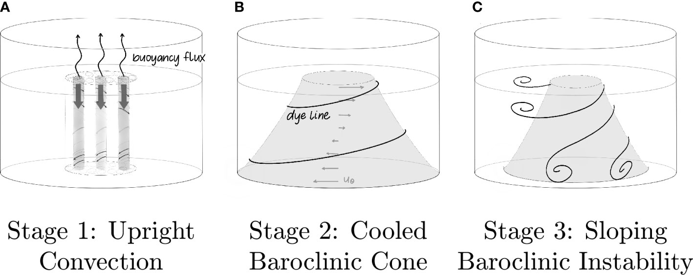
Figure 1 Schematic adapted from Marshall and Schott (1999) showing the main stages of deep ocean convection. (A) Evaporation at the ocean surface, driving convective downwelling and creating a cold column of water. (B) Vertical column of cold water becomes a cooled baroclinic cone through geostrophic adjustment; thermal wind flows develop about the baroclinic cone. (C) Thermal winds become unstable and form eddies.

With deep ocean convection as our canonical multi-scale ocean dynamics problem, we present here three separate table-top experiments each representing one of the main dynamical stages of deep ocean convection (Figure 1). It is possible to generate all three of these flows in a single, long experiment (cf. Maxworthy and Narimousa, 1994; Jacobs and Ivey, 1998; Aurnou et al., 2003; Aujogue et al., 2018). However, such experiments require carefully controlled buoyancy fluxes and thermal boundary conditions, both of which are hard to maintain using low-cost table-top devices. Instead we will model each dynamical stage of deep ocean convection via a separate experiment, each with moderately good control of the single phenomenon at hand.

Figure 1 shows illustrations of the experimental configurations used. The first experiment simulates the downwelling vertical convection phase of deep ocean convection (e.g., Haine and Marshall, 1998). This is accomplished by spraying dense dye atop the fluid surface in the center of a rotating tank of water (Figure 1A). The dye forms a gravitationally unstable top boundary layer, from which rotating convective plumes descend into the fluid bulk, similar to upright convective flows modeled in the literature (cf. Nakagawa and Frenzen, 1955; Hide and Ibbetson, 1966; Boubnov and Golitsyn, 1986; Aurnou et al., 2015; Zhang and Afanasyev, 2021). In the second and third experiments, the dye is replaced with a cold, ice-filled central cylinder (Figure 1B). The cold cylinder maintains a relatively strong, quasi-steady buoyancy flux across the fluid annulus. In slowly rotating experiments, this lateral buoyancy flux drives large-scale axisymmetric thermal winds. In more rapidly rotating experiments, the axisymmetric thermal wind flow breaks apart baroclinically to form eddies (cf. Maxworthy and Narimousa, 1994; Jacobs and Ivey, 1998; Read, 2001; Aurnou et al., 2003). See Figure 1C. In all three configurations presented here, the results match well with those of more complex experimental studies carried out in the geophysical fluids community (e.g., Matulka et al., 2016; Rodda et al., 2018).

2 The DIYnamics framework

Our team has developed a broad suite of GFD experimental hardware kits, starting first with the LEGO-based kit presented in Hill et al. (2018). They allow users to study key aspects of geophysical (and many astrophysical) fluid flows: rotating dynamics of low viscosity fluids (Cushman-Roisin and Beckers, 2011). Our DIYnamics kits can all be built from the ground-up by students or teachers alike. They are similar in scientific capability to the MIT ‘Weather in a Tank’ system (Illari et al., 2009; Marshall and Plumb, 2016). Our LEGO-based do-it-yourself (DIY) kits differ in that their parts are purchasable online with no need for custom machining or custom fabrication of the essential hardware. Additionally, the DJ table can be easily adapted from many basic record players, and does not require any machining. While the HT3 table requires some custom machining, users are able to acquire the parts from any machine shops and acrylic manufacturers. We note, however, that our favorite configurations of these kits make use of custom-built acrylic containers.

Our low-cost, do-it-yourself approach also differs significantly from the fabrication of traditional GFD experiments, which are often found only at R1 universities in GFD-focused laboratories and typically cost in the tens of thousands of dollars at the low end. The goal of the DIYnamics project is to flip that model on its head by developing less expensive, easily scalable devices that can be built and used across a wide range of educational environments.

We have developed three main series of DIYnamics hardware kits to date: The LEGO series, the DJ series, and the HT series. The kits in the LEGO series make use of an OXO rotary table. The outer rim of the rotary table is directly coupled to a drive wheel powered by a LEGO motor (Figure 2A; https://diynamics.github.io/pages/lego.html). These LEGO-based drive systems have been built by 10 year olds at outreach reach fairs in under 20 minutes. The rotation rate of the rotary table can be controlled by driving the standard LEGO motor with a variable power supply. The most recent generations of LEGO motors are programmable, and their rotation speeds can be controlled via Bluetooth connection, as will be described in the following section.

FIGURE 2

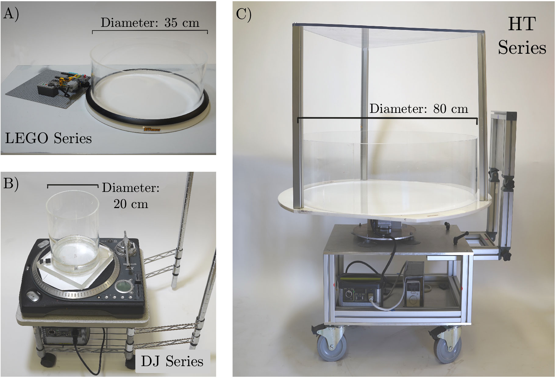
Figure 2 Images of (A) LEGO series, (B) DJ series and (C) HT3 series DIYnamics kits.

Figure 2B shows an example from the DJ series (https://diynamics.github.io/pages/dj.html). It is comprised of a disk jockey (DJ) quality record player with a cylindrical tank centered upon it. DJ turntables, such as the Numark TTX shown, have rotation rates that can range from 17 to 117 revolutions per minute (RPM), which maintain rotational stability to within 1 part in ${10}^4$. By placing the turntable on a rolling cart, this system can be easily rolled in and out of classrooms. Including a portable battery on the cart allows the system to be self-contained, with no power chords for students to trip over.

Figure 2C shows the HT3, the latest member of the HT series of DIYnamics rotating tables (https://diynamics.github.io/pages/ht3.html). The HT3 is currently the largest DIYnamics kit, with its 80 cm tank. This tank sits upon a brushless servo-driven pedestal with rotation rates from 0.16 up to 13.33 RPM. It has an upper deck that can be used for holding cameras and cell phones as well as other possible measurement equipment. In addition, we designed a dedicated cart for it with sturdy, large-diameter, lockable wheels, which makes it ideal for rolling outside over uneven pavement, as is often necessary at public outreach events and the like.

2.1 The LEGO SPIKE set up

The three desktop experiments carried out here are made using the LEGO SPIKE Kit (Figure 3), which is the newest LEGO series kit, built around LEGO’s SPIKE Prime robotics kit. While the DJ and HT3 kits have better rotational stability and finer rotational control, we use the LEGO kit to show that it is possible to generate all three deep ocean convection flows using one of the LEGO series kits, which are the simplest and most ‘DIY’ of our different systems.

FIGURE 3

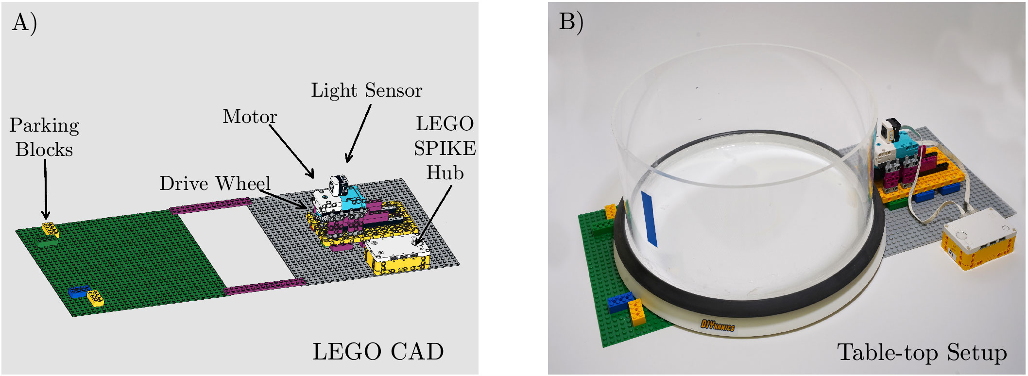
Figure 3 (A) Rendering of the LEGO SPIKE kit made using the Brick Studio LEGO CAD software. (B) Image of the SPIKE set up, including OXO turntable on a table-top.

The LEGO-based kits provide students the broadest range of learning and engagement opportunities. First, students can build the LEGO kits from the ground up, using, for example, the detailed BrickStudio build instructions given here in the Supplementary Materials (Figure 3A). Second, the SPIKE motor can be programmed using the LEGO SPIKE app, providing an opportunity for students to program a real-world, physical experimental system using either the graphical language Scratch or the structured language microPython. The LEGO SPIKE Kit allows students to build up a range of hands-on engineering and coding skills. Students can additionally take data directly via the SPIKE’s Hub microcontroller. By placing the SPIKE’s light sensor atop the motor in conjunction with a piece of colored tape on the tank sidewall (see Figure 3B), it is possible to program the SPIKE to acquire measurements of the tank’s rotation period. Example Scratch and microPython codes that rotate the tank and acquire rotation period data can be found at https://github.com/rachtrip/DIYnamics-LEGO-SPIKE.git.

Any container that fits on the OXO can be used, but for our experiment, we maximize space by installing an acrylic sidewall that is nearly equal to the OXO’s inner diameter. The LEGO system that we present here requires the acrylic sidewalls are secured onto the OXO turntable using silicone or epoxy (e.g., https://youtu.be/sN1ahWml17w). Note that it takes one to two days for most silicones or epoxies to fully cure, so this step should be done before students follow the supplementary BrickStudio instructions to build the LEGO SPIKE kits in the classroom.

All the images and videos shown in this paper have been acquired using cameras situated in the non-rotating lab frame. However, we have ways to view the experiments in the rotating frame. For instance, a gooseneck clamp can be used to hold a camera in the rotating frame. Placing a sheet of paper on the outside of the tank, opposite of the location of the camera removes the apparent spinning of the background (e.g., https://youtu.be/jX5ppPQaea4). Side views are most useful in thermal wind experiments, allowing students to see the thermal wind shear clearly.

To view the experiment in top view, place a camera above the rotating tank’s axis of rotation. This top view camera can be situated in the rotating frame using a gooseneck clamp or it may be situated in the lab frame. Since it is typically simpler and faster to set up the camera in the lab frame, we have developed an associated web-served app, DIYrotate, that digitally transforms the axial rotation rate in a given top view digital movie (https://DIYnamics.github.io/pages/diyrotate.html). Using DIYrotate, it is possible to transform lab frame camera footage into the tank’s rotating frame (e.g., https://youtu.be/u6OoYdrYZ0o). When carrying out experiments, experimenters can measure the tank’s rotation period using the SPIKE light sensor or by using a stopwatch to measure it by hand and supply that as input to DIYrotate.

Leveling the tank will minimize the amplitude of surface waves that that are not being simulated here. The tank can be leveled incrementally by using shims (e.g., playing cards) and a bubble level. Alternatively, the tank can left unleveled, which can facilitate discussion of waves and inertial modes in rotating systems.

Before actually adding dye to the fluid, it is essential that all the water in the tank is rotating at the same angular velocity as the tank. This state of the fluid is called solid body rotation. If the water is not in solid body rotation, the ensuing experiments rarely work correctly. Spin-up in these experiments occurs via an approximately exponential response that occurs on the time scale (Warn-Varnas et al., 1978; Duck and Foster, 2001):

$\begin{array}{ll}{\tau }_{su}\simeq \frac{H}{{(\nu \Omega )}^{1/2}}=\frac{3.1H}{{(\nu {\mathcal{N}}_{RPM})}^{1/2}},& (1)\end{array}$

where $H$ is the depth of the fluid layer, $\nu$ is the kinematic viscosity of the working fluid (${10}^{-6}$ m²/s for room temperature water), $\Omega =2\pi /{\tau }_{\Omega }$ is the tank’s angular rotation velocity that can be recast in terms of revolutions per minute as

$${\mathcal{N}}_{RPM}=\frac{60}{{\tau }_{\Omega }}=60\frac{\Omega }{2\pi },$$

with ${\tau }_{\Omega }$ being the tank’s rotation period in seconds. Based on our experience, the fluid is adequately spun-up when the system rotates for $5{\tau }_{su}$ before starting a given experimental case. Figure 4 shows this wait time plotted as a function of ${\mathcal{N}}_{RPM}$ for $H=5$ and 10 cm fluid layer depths.

FIGURE 4

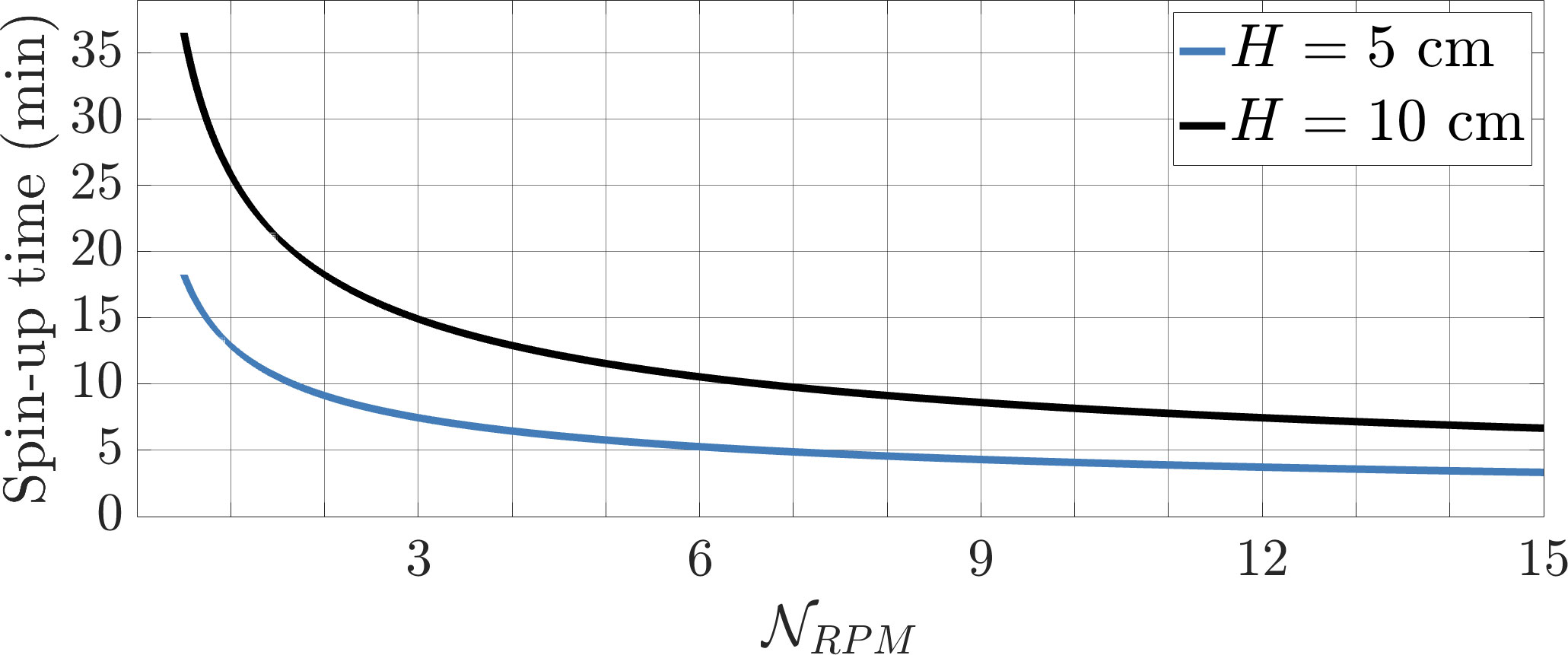
Figure 4 Estimated spin-up equilibration time,$5{\tau }_{su}$, plotted as a function of tank rotation rate, ${\mathcal{N}}_{RPM}$, for $H=5$ and $10$cm fluid layer depths.

The reader is directed to the ‘Tips’ page on the DIYnamics site for further ideas on how best to optimize the experiments (https://diynamics.github.io/pages/tips.html).

3 Desktop models of deep ocean convective flows

3.1 Experiment 1: downwelling dye-driven convection

Desktop simulations of the upright convection phase of deep ocean convection are made by filling the OXO tank with 10 cm of water and rotating the SPIKE motor at its maximum rate, which corresponds to a rotation period of ${\tau }_{\Omega }=5.36$ seconds for the drive wheel employed here. Thus, the tank spins at

$\begin{array}{ll}{\mathcal{N}}_{\mathrm{RPM}}=10.26\text{\hspace{0.17em}RPM},& (2)\end{array}$

corresponding to an angular velocity of

$\begin{array}{ll}\text{Ω}=\frac{\pi {\mathcal{N}}_{\mathrm{RPM}}}{30}=1.07\text{\hspace{0.17em}rad}/\text{s}.& (3)\end{array}$

In order to create a controllable localized central dye patch, we place a 6.4 mm thick acrylic sheet over the top of the tank, with an 11 cm centered thru hole cut out of it see Figure S1B. Once the fluid has spun-up, we spray dense food dye through the hole in the sheet. The sheet is then removed and we image the subsequent evolution of the $\approx 15$cm diameter dye patch.

The food dye acts as a proxy for the cold, dense surface waters that become convectively unstable in deep ocean convection events. The convective forcing is often described by the non-dimensional Rayleigh number,

$\begin{array}{ll}Ra=(\delta \rho /\rho )g{H}^3/(\nu \kappa )\simeq 2\times {10}^9,& (4)\end{array}$

which estimates the ratio of buoyancy versus diffusional effects. Here, $g=9.8$m/s² is gravity, $\delta \rho /\rho =({\rho }_{dye}-\rho )/\rho =0.007$is the density of anomaly of the food dye relative to pure water, where our dye density is measured to be ${\rho }_{dye}=1.007$ g/cm³ and we take $\rho =1$ g/cm³ as the density of water. The axial depth of the fluid layer is $H=10$cm, $\nu ={10}^{-6}$m²/s is the kinematic viscosity of water, and $\kappa \sim 3\times {10}^{-8}$ m²/s is estimated to be the chemical diffusivity of the food dye. The strength of rotational effects is characterized by the non-dimensional Ekman number,

$\begin{array}{ll}Ek=\nu /(2\text{Ω}{H}^2)=15\nu /(\pi {\mathcal{N}}_{RPM}{H}^2)=4.7\times {10}^{-5},& (5)\end{array}$

which estimates the ratio of viscous and Coriolis forces. The working fluid’s material properties are cast in terms of the Prandtl number,

$\begin{array}{ll}Pr=\nu /\kappa \simeq 30.& (6)\end{array}$

The regime of rotating convection is often characterized in terms of the so-called convective Rossby number, $Ro$, which estimates the local convective scale ratio of inertial and Coriolis accelerations (Aurnou et al., 2020). When Ro ≲ 1, Coriolis accelerations dominate, generating rotationally aligned convective flow structures (e.g., Nakagawa and Frenzen, 1955). Here, the convective Rossby number value is estimated to be

$\begin{array}{ll}Ro=\sqrt{RaE{k}^2/Pr}\simeq 0.1.& (7)\end{array}$

The $Ra$ and $Ro$ values are likely upper bounds since we use an impulsive flux of dye to force the flow in this experiment. Even so, $Ro$ remains less than unity, such that we expect rotational effects to dominate the convection dynamics. Furthermore, the $Ra$, $Ek$ and $Ro$ values employed in this experiment are in adequate agreement with the deep ocean convection simulations carried out by Jones and Marshall (1993); Klinger and Marshall (1995) and Pal and Chalamalla (2020).

Rotationally dominated convection occurs in the form of tall columnar flows that can be $O(H)$ in axial extent. In contrast, these columnar structures are narrow in the cross-axial, or horizontal, direction. At the onset of convection, linear theory predicts the horizontal scale of the convective cells will have a radius of

$\begin{array}{ll}{r}_{conv}=1.2E{k}^{1/3}H=1.2{ \left(\frac{\nu }{2\Omega H^2}\right)}^{1/3}H=1.2{\left(\frac{15\nu H}{\pi {\mathcal{N}}_{RPM}}\right)}^{1/3},& (8)\end{array}$

(Julien and Knobloch, 1998; Horn and Aurnou, 2022). For our dye-driven rotating convection experiment, we predict that $r_{conv}\simeq 0.43$ cm, such that we estimate that 17 structures will form across the $r_{patch}\simeq$7.5 cm dye patch (Figure 5A and its inset). These initial convective structures later ‘plump up’, as shown in Figure 5B, to a larger, turbulent horizontal scale once the convection has become fully developed (Fernando et al., 1991; Guervilly et al., 2019; Aurnou et al., 2020; Bire et al., 2022).

FIGURE 5

Figure 5 (A) Linear stability predictions of horizontal cell radius $r_{conv}$ of rotating convective flows plotted versus the tank’s rotation rate given in terms of ${\mathcal{N}}_{RPM}$. (B) Estimated number of rotating convection structures, $r_{patch}/r_{conv}$, forming out of the emplaced dye patch versus ${\mathcal{N}}_{RPM}$. In this experiment, the diameter of the dye patch is $2r_{patch}=15$ cm and the fluid layer depth is $H=10$ cm. The vertical dashed line indicates the ${\mathcal{N}}_{RPM}=10.26$, which corresponds to the rotation rate of the upright convection experiment presented herein.

Figure 6 shows images of rotating convection forming from a dense dye patch sprayed at the top surface of the fluid layer. The top row shows top view images at two points in time; the bottom row show the accompanying, contemporaneous side view images. Also see Supplementary Movie 1, from which these images are derived. Panels a) and c) show the dye field roughly 10 rotation periods after the emplacement of the dye. Panels b) and d) show images acquired roughly 45 rotation periods after dye emplacement. The dye converges in downwelling plumes, each of which act to generate positive axial vorticity via stretching of the background vorticity. This positive local vorticity causes the dye to swirl counter-clockwise, in the same direction as the tank is rotating. Approximately 15 - 20 structures span the diameter of the dye patch in panel a, in adequate agreement with (8). In panels b) and d), the dye extends across the entire depth of the fluid layer, forming a well-defined dye “chimney”. The chimney as well as the individual convective flow structures within the chimney remain aligned along the direction of the rotation axis. Roughly 6 or 7 convective structures span the dye patch, showing that the horizontal scaleincreases as flow becomes fully developed, in qualitative agreement with theory. Unlike the upright convective structures, the diameter of the larger-scale chimney remains the same throughout this experiment.

FIGURE 6

Figure 6 Table-top experimental simulation of the initial upright convective phase of deep ocean convection. The water depth is $H=10$ cm; the rotation rate is 11.2 RPM such that ${\tau }_{\text{Ω}}=5.36$ s. The patch of dye at the fluid surface has an approximate diameter of 15 cm. (A, C) Top and side views, respectively, of the intial downwelling flow pattern roughly 10 ${\tau }_{\text{Ω}}$ after dye patch emplacement. (B, D) Fully-developed flow $\approx 45{\tau }_{\text{Ω}}$ after dye emplacement. (Still images harvested from Supplementary Movie 1.).

3.2 Thermally-driven annular flows

After the initial upright convection stage of deep ocean convection (Figure 1A) there exists a cold chimney of fluid that spans the full depth of the ocean. This is represented in our table-top experiments by the dense dye chimney in Figure 6D. This dye chimney will continue to evolve, developing azimuthal thermal winds and baroclinic instabilities given sufficient time (e.g., Maxworthy and Narimousa, 1994). Strongly unstable dye-driven baroclinic flows would, however, require us to either use denser dye or to continually flux dye into the patch. Instead, in the following experiments, we simulate the later, post-upright-convective stages of deep ocean convection (Figures 1B, C) by replacing the dye chimney in Figure 6D with a comparable radius can, or jar, of ice water that generates strong thermally-driven flows around its edge, as shown schematically in Figure 1B.

The existence of the centered cold source changes the geometry of the experiment. The working fluid is no longer simply connected and exists now in the form of a cylindrical annulus, corresponding to the classical configuration known as Hide’s annulus (e.g., Ghil et al., 2010). The radius of the centralized cold can sets the inner radius of the fluid annulus, $R_i$, while the tank sidewall sets the fluid’s outer annular extent, $R_o$. The fluid that sits laterally adjacent to the ice-filled can at $r\simeq R_i$ represents the dense fluid in the outer part of the deep ocean convective chimney. The warmer fluid further away in radius represents the surrounding ambient ocean water. Estimates for the input scales in the annulus experiments are provided in Table 1.

TABLE 1

Table 1 Parameter estimates for the annular thermal wind (TW) and baroclinic instability (BCI) experiments.

3.3 Experiment 2: Axisymmetric thermal wind flows

The Rossby number in all three experiments is small, $Ro⪅1$, which implies that Coriolis accelerations dominate the dynamics. Thus, the leading order terms in the momentum balance represent a geostrophic balance between Coriolis and pressure gradient forces, and the leading order terms in the vorticity equation are the Coriolis and buoyancy terms:

$\begin{array}{ll}2\text{Ω}·\nabla u=-g\times \nabla (\rho /{\rho }_o),& (9)\end{array}$

which is referred to as a geostrophic balance (McWilliams et al., 2006; Cushman-Roisin and Beckers, 2011; Marshall and Plumb, 2016). In (9), $\text{Ω}$ is the system’s rotational angular velocity vector, $u$ is the fluid velocity measured in the rotating frame, $g$ is lab gravity, $\rho$ is the fluid density, and ${\rho }_o$ is a reference density of the ambient fluid. In right-handed cylindrical coordinates ($r$, $\theta$, $z$), the angular velocity and gravity vectors are axial, $\text{Ω}=\text{Ω}\widehat{z}$ and $g=g\widehat{z}$, allowing (9) to be recast as

$\begin{array}{ll}2\text{Ω}\frac{\partial u}{\partial z}=-\frac{g}{{\rho }_o}(\widehat{z}\times \nabla \rho ),& (10)\end{array}$

known as ‘thermal wind’ balance. The left hand side of (10) describes vorticity generation by stretching of the so-called planetary vorticity, $2\Omega$, and the right hand side is the baroclinic torque generated by lateral gradients in fluid density.

In the absence of salt the incompressible equation of state for water is

$\begin{array}{ll}\rho (T)={\rho }_0(1-\alpha (T-T_0)),& (11)\end{array}$

where $\alpha \simeq 2\times {10}^{-4}$ 1/K is its thermal expansion coefficient, $T$ is the fluid temperature, $T_0$ is ambient temperature, and ${\rho }_o=\rho (T_o)$ is the ambient density. Substituting (11) into (10) then yields

$\begin{array}{ll}\frac{\partial u}{\partial z}=\frac{\alpha g}{2\Omega }(\widehat{z}\times \nabla T).& (12)\end{array}$

Lastly, taking into account that the temperature gradient in our cylindrical annular experiments is predominantly radial, $T\approx T(r)$, the thermal winds will satisfy

$\begin{array}{ll}\frac{\partial u_{\theta }}{\partial z}=\frac{\alpha g}{2\Omega }\frac{\partial T}{\partial r}.& (13)\end{array}$

The above equations show that horizontal density gradients lead to a vertical shearing of the horizontal flow fields in rapidly rotating fluids, as illustrated in Figure 1B. In a non-rotating system, a radial density gradient would generate an axisymmetric, meridionally-overturning circulation. In rapidly rotating low $Ro$ systems, the radial density gradients generate baroclinic torques that drive an axially-shearing azimuthal velocity field, $d{u}_{\theta }/dz$. The thermal wind shear in right-handed systems ($\text{Ω}>0$) is positive $d{u}_{\theta }/dz>0$ since $dT/dr>0$. From (13), the azimuthal thermal wind velocity at the top of the fluid layer will super-rotate with respect to the tank, and the fluid at the bottom of the fluid layer will tend to sub-rotate relative to the tank. Thus, in an experiment with a right handed angular rotation velocity, a dyed column of fluid observed in the rotating frame should tend to be sheared in a right handed sense as well, with the fluid at the top precessing in the prograde + $\widehat{\theta }$-direction. The $\partial u_{\theta }/\partial z$ shearing of the thermal wind field will act to continually wrap the dye column around the domain, so long as the compositionally-dense dye doesn’t settle under its own weight and the effects of Ekman pumping. Thus at the bottom of the tank, the fluid processes about the baroclinic cone in the retrograde direction. This non-intuitive axial shearing of the azimuthal thermal wind flow field is the rotating fluid analog to the precession of a tipped, rapidly rotating gyroscope (Haine and Cherian, 2013).

Figure 7 shows the results of a thermal winds experiment. The water depth in this experiment is $H=10$ cm, with a rotation rate of approximately 1.46 RPM. The system was allowed to spin up without ice in the inner can for approximately 30 minutes to allow for solid body rotation. Ice, salt, and water were added to the can after spin-up and the system was allowed to establish a thermal gradient for approximately 5 minutes. To estimate the timescale that the thermal wind flow will take to wrap around the can in this experiment, we calculate thermal wind velocity $U_{TW}$ and determine the time ${\tau }_{TW}$ that it takes to flow around the $R_i$radius can:

FIGURE 7

Figure 7 Side-view images showing evolution of an initially vertical dye line in a thermal wind flow field. (A) Initial dye emplacement adjacent to the cold central can. Panels (B–D) show successive wrappings of the dye around the can by the ∂uθ/∂z thermal wind shear (13). (Still images harvested from Supplementary Movie 2).

$\begin{array}{ll}{\tau }_{TW}=\frac{2\pi R_i}{U_{TW}}.& (14)\end{array}$

The thermal wind velocity scales as,

$\begin{array}{ll}{U}_{TW}=\frac{d{u}_{\theta }}{dz}H=\frac{\alpha g}{2\Omega }\frac{\partial T}{\partial r}H\simeq \frac{\alpha gH\Delta T}{2\Omega \Delta R}\approx 1.5\text{\hspace{0.17em}cm}/\text{s},& (15)\end{array}$

where we have used laboratory measurements of $\Delta T=T_i-T_o=2.7\pm 0.2$ K (see Figure S4C in the Supplementary Materials) and $\Delta R=R_o-R_i=12$. Equations 14 and 15 then give the wrapping timescale,

$\begin{array}{ll}{\tau }_{TW}=\frac{4\pi \Omega R_i}{\alpha gH(\partial T/\partial r)}\approx 23 \text{s},& (16)\end{array}$

over which the vertical thermal wind shear flow should wrap the dye once around the can.

Figure 7A shows the dye as it was dropped into the tank adjacent to the inner cylinder. The thermal wind vertically shears the dye, causing it to circulate in the prograde direction at the top of fluid layer and in the retrograde direction near the tank bottom. Over time, the thermal winds wrap the dye in successive windings around the inner cylinder. Figures 7B–D show the dye pattern at 2, 4, and 6 wrapping times, successively, which correspond to 40, 80, and 120 seconds after the dye is first added to the tank. The experimental measurements of the wrapping timescales are approximately one wrap at 26 s, two wrappings after 56 s, and a third wrapping at 82 s, giving an average experimental wrapping time of $28\pm 2$ s, in good zeroth order agreement with the estimate given in (16).

There are several factors that affect the thermal wind wrapping timescale in any given experiment. The primary factor is the extent of the temperature gradient $\partial T/\partial r$. The approximation used here is that the temperature gradient covers the half the width of the tank. In contrast, if the temperature gradient is better described over the full width of the annulus, that would correspond to a doubling of the wrapping timescale. Additionally, we expect that the thermal gradient will change over time both as a consequence of the thermally-driven radial overturning circulation and due to the continual melting of the ice in the central cold can. As $\Delta T$ decreases over time, the wrapping timescale ${\tau }_{TW}$ will increase, which can eventually lead to baroclinic instability as considered in the following section.

3.4 Experiment 3: Baroclinic Instability

The Coriolis-dominated azimuthal thermal wind flow supports the colder, denser fluid adjacent to the central cylinder, nearly shutting down vertical motions in the fluid through hydrostatic balance. However, due to the sloping density surfaces, the density field stores gravitational potential energy. In some cases, this gravitational potential energy can be released through perturbations to the thermal wind flow via a process called barolinic instability (BCI) (e.g., Phillips, 1956; McWilliams et al., 2006; Vallis, 2017). When BCI occurs, the available potential energy is converted to kinetic energy in the form of “sloping convection”. In our table-top rotating tank experiments, these BCI phenomena take the form of non-axisymmetric vortices, or eddies, which are easily visualized with dye.

The theory of BCI has been well studied in both atmospheric (e.g., Eady, 1949; Charney and Stern, 1962; Farrell, 1982; Eliassen, 1983), and oceanic frameworks (e.g., Gill et al., 1974; Robinson and McWilliams, 1974; Molemaker et al., 2005; Tulloch et al., 2011), as well as in other more exotic planetary and astrophysical settings (e.g., Tobias et al., 2007; Lonner et al., 2022). In this paper, we take advantage of the stability properties of the Eady problem (e.g., Eady, 1949; Vallis, 2017). As in Vallis (2017), we make the following assumptions to use stable solutions to the Eady problem: (i) there are no so-called $\beta$-effects, $\beta =0$; (ii) the basic state has uniform shear; (iii) the motion is contained between a flat horizontal bottom and a flat rigid lid; and (iv) there is a constant vertical density stratification, $\partial \rho /\partial z$, of the fluid. Our DIYnamics setup satisfies criteria (i)–(iii). It is possible that $T$, and thus $\rho$, evolve over time. However, the thermometry data in Supplementary Materials Section 3 shows that such secular changes in the mean temperature fields are small over the lifetimes of the experiments.

Linear analysis of BCI predicts its characteristic scale to be set by the Rossby radius of deformation, defined as

$\begin{array}{ll}{R}_{def}=\frac{N_{b}H}{2\Omega },& (17)\end{array}$

where

$\begin{array}{ll}{N}_b=\sqrt{-\frac{g}{{\rho }_0}\frac{\partial \rho }{\partial z}}=\sqrt{\alpha g\frac{\partial T}{\partial z}},& (18)\end{array}$

is the buoyancy, or Brunt-Vaisala, frequency (e.g., Sutherland, 2010; Cushman-Roisin and Beckers, 2011). By taking $\partial T/\partial z\approx \text{Δ}T/H$ in (18) where $\text{Δ}T=T(R_o)-T(R_i)$ is the temperature difference across the annular gap, the radius of deformation becomes

$\begin{array}{ll}{R}_{def}=\frac{\sqrt{\alpha g\Delta TH}}{2\Omega }=\frac{15}{\pi }\frac{\sqrt{\alpha g\Delta TH}}{{\mathcal{N}}_{RPM}}.& (19)\end{array}$

Stability theory further predicts that baroclinic instabilities will develop with a characteristic time scale

$\begin{array}{ll}{\tau }_{BCI}=3\frac{R_{def}}{U_{TW}},& (20)\end{array}$

with the prefactor value taken from Sloyan and O’Kane (2015). The diameter of the instability is determined by the fastest growing baroclinic mode to be $\approx 4R_{def}$ via analysis of the dispersion relationship to the linearized quasi-geostrophic equations (e.g., Vallis, 2017). Expressions (20) and (15) then yield

$\begin{array}{ll}{\tau }_{BCI}\simeq \frac{3L_{gap}}{\sqrt{\alpha g\Delta TH}}\approx 22 \text{s},& (21)\end{array}$

in our annulus experiments, where $L_{gap}=R_o-R_i\simeq 12$ cm, $H=5$ cm and we estimate $\Delta T\approx 2.9$ K based on the Figure 4D thermometry data in the Supplemental Materials. This ${\tau }_{BCI}$ value approximates the time over which thermal wind flows will tend to destabilize in the experiment. Note that the growth time scale does not depend on $\Omega$, which implies that baroclinic instabilities should develop over roughly the same time period in all our annulus experiments since $\Delta T$ remains roughly constant and the fluid geometry is also held fixed in these cases.

In addition to requiring sufficient time for the instabilities to grow, there needs to be sufficient space in the fluid annulus as well. Thus, thermal winds can only become baroclinically unstable if the fluid gap is significantly larger than the instability scale $4R_{def}$. Alternatively, one can ensure that the thermal wind flow remains stable by using a small enough diameter tank. Conversely, in a large diameter tank (e.g. the HT3), a very slow rotation rate is necessary to maintain a balanced thermal wind flow.

We will estimate that baroclinic instability is possible in our tanks given the condition that

$\begin{array}{ll}4R_{def}⪅L_{gap}.& (22)\end{array}$

Recasting (22) in terms the system’s angular rotation rate shows that BCI can only develop when the tank’s rotation rate exceeds

$\begin{array}{ll}{\text{Ω}}^{crit}\approx 2\frac{\sqrt{\alpha g\Delta TH}}{L_{gap}},& (23)\end{array}$

which corresponds to

$\begin{array}{ll}{\mathcal{N}}_{RPM}^{crit}\approx \frac{60\sqrt{\alpha g\Delta TH}}{\pi L_{gap}}=2.6,& (24)\end{array}$

where we have used $H=5$ cm, $L_{gap}=12$ cm, and $\text{Δ}T\approx 2.9$K based on Figure S4D. Below this rotation rate, the thermal winds in the table-top experiments should remain stable and nearly axisymmetric, whereas at higher rotation rates the thermal wind flow should break apart into a set of baroclinic eddies of diameter $\approx 4R_{def}$ on the ${\tau }_{BCI}$ scale (e.g., Eady, 1949; Pierrehumbert and Swanson, 1995; Read, 2001).

The BCI that develop in our experiments first develop adjacent to the cold source. To predict the number of initial structures that form, we use the inner radius as the radius of the cold boundary layer. At later times, the instabilities of the mean flow, visualized as eddies, will grow to fill the annulus. The initial number of baroclinic eddy structures is predicted to be

$\begin{array}{ll}{m}_{BCI}\simeq \frac{2\pi R_i}{4R_{def}}=\frac{\pi R_i\Omega }{4\sqrt{\alpha g\Delta TH}}\approx \frac{{\pi }^2{R}_i{\mathcal{N}}_{RPM}}{60\sqrt{\alpha g\Delta TH}}.& (25)\end{array}$

Figure 8 shows the results of two baroclinic instability experiments. The water depth in this experiment was 5cm, with two rotation rates of approximately 3.9 and 11 RPM. The system was allowed to spin up for approximately 10 minutes to achieve solid body rotation. Ice, salt, and water were added to the can after spin-up and the system was allowed to establish a thermal gradient for approximately 3 minutes ($\approx 9{\tau }_{BCI}$) before dye was added to the tank. A few drops of blue dye were then added adjacent to the cold can, and a few drops of red dye were added near the outer radius of the tank (see Supplementary Movies 3 and 4).

FIGURE 8

Figure 8 Top-view images of baroclinic instability experiments. The top row images (A–C) correspond to an experiment rotated at 3.9 revolutions per minute. The bottom row images (D–F) correspond to an experiment rotated at 11.0 revolutions per minute. In both rows, the time from ice emplacement in the central cylinder increases from left to right as (A, D) $t\simeq 2{\tau }_{BCI}$, (B, C) $t\simeq 4{\tau }_{BCI}$, and (C, F) $t\simeq 10{\tau }_{BCI}$. In both experiments, $H\simeq 5$, and ${\tau }_{BCI}\simeq 22$ s. The approximate length-scale twice the radius of deformation, $4R_{def}$ is annotated in panels (B, D). (Images harvested from Supplementary Movies 3 and 4).

Figures 8A–C show the experiment run at 4 RPM, and Figures 8D–F show the BCI experiment at 11 RPM at ${\tau }_{BCI}\simeq 2,4,$ and 10, respectively. (Also see Supplementary Movies 3 and 4 from which these figures are derived.) In both experiments, the flow is baroclinically unstable. Early stages of the experiment ($t/{\tau }_{BCI}$ = 2) show the baroclinic modes develop near the cold can with little perturbation of the red dye in the outer portions of the annulus. Three baroclinic modes develop in the 4 RPM experiment, whereas 5 modes develop in higher rotation rate experiment. The increase in baroclinic modes with rotation rate qualitative agrees with (24).

Figure 9 shows the predictions for our thermal wind flows and baroclinic instabilities plotted versus tabletop experimental measurements. Panel a) shows the number of dye wrappings as a function of time in the thermal winds experiment. The solid black line shows the predicted number of wrappings via (14) using the temperature gradient measured across the fluid gap in the thermometry experiment shown in Figure S4. The three black circles are our estimated wrapping time estimates made using the Supplemental Material’s dye visualization movie 2.The dashed line shows the best fit inversion for the temperature gradient in the experiment.

FIGURE 9

Figure 9 Quantitative comparisons between table-top thermal annulus experiments and theory. (A) Dye wrappings in Figure 7 dye to thermal wind shear. (B) Baroclinically unstable modes, $m_{bci}$, as a function of rotation rate.

Figure 9B shows the visual measurements of $m_{BCI}$from the Supplementary BCI movies plotted versus the rotation rate of the tank in revolutions per minute (black circles). The solid black line denotes the theoretical prediction (24) $\text{Δ}T=T_i-T_o=2.9\pm 0.3$ K measured in Figure S4D. The dashed and dotted lines show best fit $\text{Δ}T$ estimates for the experimental cases.

While there is good agreement in Figure 9 between theory and observations, the inversions for both TW and BCI shows that our margin of error in $\text{Δ}T$ ranges up to $\approx 1.5$ K. This suggests that our assumption that the temperature gradient spans the entire annulus may be too simple. Despite this, Figure 9 demonstrates that our table-top geophysical fluids experiments yield results that can compared with theory.

4 Discussion

This study demonstrates that multi-scale deep ocean convection processes crucial to the behavior of deep ocean overturning and, thus, to global climate, can be successfully modeled using small-scale table-top LEGO-based hardware kits. Given the capabilities of our DIYnamics setup, we model deep ocean convection through three controlled experiments: upright convection, thermal wind flows, and geostrophic adjustment through baroclinic instability. Linear theory is presented that adequately predicts the characteristic flows and flow structures.

Our experiments have several tunable parameters that allow experimentalists to change dynamical regimes. In the experiments presented here, it is easiest to alter the depth of the fluid layer, H, and the rotation rate of the tank, N_RPM. It is however also possible to alter the temperature gradient by using different quantities of ice, for example. Furthermore, adding a vertical stratification profile to the working fluid creates a more realistic (and more complex) ocean model (e.g., Christin et al., 2021; Stewart et al., 2021).

Figure 10 shows the variety of DIYnamics experiments already being carried ‘in the wild.’ With their relatively cost-effective materials, these kits can be used in classroom and outreach settings that would not normally have access to geophysical fluid dynamics and climate experimentation. Our experiments provide tangible, human-scale representations of phenomena essential to understanding global-scale climate and climate change. Further, they engage scientists, and future scientists, across all levels and encourage discussion in all the settings where they are used.

FIGURE 10

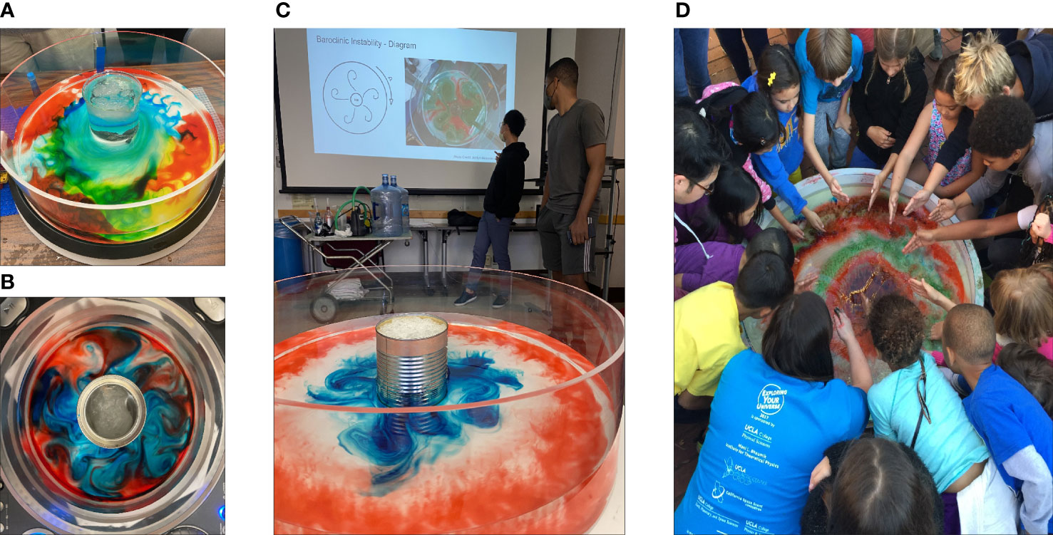
Figure 10 DIYnamics in the wild. (A) Oblique view of a mixed thermal wind-evaporative convective multi-scale "ow in a LEGO tank in Fall 2022 AOS/EPSS M71 undergraduate computing class at UCLA. (B) Baroclinic instability (BCI) on the DJ table, top view image courtesy of Vincent Caiazzo. (C) Student-led HT3 BCI experiments in UCLA’s Fall 2021 graduate-level Introduction to Atmospheric and Oceanic Fluid Dynamics (AOS 200A) course. (D) Early career scientists simulating Jupiter’s great red spot at UCLA’s 2018 Exploring Your Universe (EYU) science outreach event.

Towards that end, the Supplementary Materials contains a detailed, robust recipe for each of the three experiments presented here. Note though that there are innumerable ways to carry out these experiments. With experience, most users come up with their own individualized set of steps. The goal of this work is just to get everyone actively experimenting.

Data availability statement

The original contributions presented in the study are included in the article/Supplementary Material. Further inquiries can be directed to the corresponding author.

Author contributions

JM, RT, and JA designed the study, conducted all the experiments, created the figures, and wrote the manuscript. RT developed the current LEGO SPIKE kit, based on an initial design concept and fabrication by WC using a LEGO EV3 robotics kit. RT created build instructions, set-up the filming, and edited all movies. NK, SH, and JA developed the LEGO Series. HG, TL, and JA developed the DJ and HT Series DIYnamics Kits. SC developed the DIYrotate software employed in the supplemental movies and the analysis thereof. All authors co-edited the manuscript. All authors contributed to the article and approved the submitted version.

Funding

We gratefully acknowledge the support of the National Science Foundation by awards OCE–PRF #2205637 (JM), EAR #1853196 and #2143939 (JA). In addition, our participation at the 2022 Earth Educators’ Rendezvous was supported by NSF EAR and AGS funding. JM’s development of undergraduate and graduate level DIYnamics demonstrations was supported by UCLA’s Center for the Advancement of Teaching’s Instructional Improvement Program award #21-08.

Acknowledgments

We thank the organizers and participants of the Earth Educator’s Rendezvous 2022 and of UCLA’s Exploring Your Universe, and the UCLA students in (Fall 2021 AOS 200A and Fall 2022 AOS/EPSS M71. JM would like to thank Andrew Stewart and Gang Chen for co-sponsorship on her Instructional Improvement Grant. We would also like to thank Andrew Stewart, Marcelo Chamecki, and Jonathan Mitchell for furiously $\beta$-testing our experiments in their classes. Alex Gonzalez, J. Paul Mattern, Juan Lora, Hearth O’Hara , David James and Sam May are also warmly acknowledged for their various contributions. We also thank the two reviewers whose helpful comments and suggestions improved this manuscript.

Conflict of interest

The authors declare that the research was conducted in the absence of any commercial or financial relationships that could be construed as a potential conflict of interest.

Publisher’s note

All claims expressed in this article are solely those of the authors and do not necessarily represent those of their affiliated organizations, or those of the publisher, the editors and the reviewers. Any product that may be evaluated in this article, or claim that may be made by its manufacturer, is not guaranteed or endorsed by the publisher.

Supplementary material

The Supplementary Material for this article can be found online at: https://www.frontiersin.org/articles/10.3389/fmars.2023.1192056/full#supplementary-material

References

Aujogue K., Pothérat A., Sreenivasan B., Debray F. (2018). Experimental study of the convection in a rotating tangent cylinder. J. Fluid Mech. 843, 355–381. doi: 10.1017/jfm.2018.77

CrossRef Full Text | Google Scholar

Aurnou J., Andreadis S., Zhu L., Olson P. (2003). Experiments on convection in earth’s core tangent cylinder. Earth Planet. Sci. Lett. 212, 119–134. doi: 10.1016/S0012-821X(03)00237-1

CrossRef Full Text | Google Scholar

Aurnou J., Calkins M., Cheng J., Julien K., King E., Nieves D., et al. (2015). Rotating convective turbulence in earth and planetary cores. Phys. Earth Planet. Interiors 246, 52–71. doi: 10.1016/j.pepi.2015.07.001

CrossRef Full Text | Google Scholar

Aurnou J. M., Horn S., Julien K. (2020). Connections between nonrotating, slowly rotating, and rapidly rotating turbulent convection transport scalings. Phys. Rev. Res. 2, 043115. doi: 10.1103/PhysRevResearch.2.043115

CrossRef Full Text | Google Scholar

Bire S., Kang W., Ramadhan A., Campin J.-M., Marshall J. (2022). Exploring ocean circulation on icy moons heated from below. J. Geophys. Res.: Planets 127, e2021IJE007025.

Google Scholar

Boubnov B., Golitsyn G. (1986). Experimental study of convective structures in rotating fluids. J. Fluid Mech. 167, 503–531. doi: 10.1017/S002211208600294X

CrossRef Full Text | Google Scholar

Charney J. G., Stern M. E. (1962). On the stability of internal baroclinic jets in a rotating atmosphere. J. Atmos. Sci. 19, 159–172. doi: 10.1175/1520-0469(1962)019<0159:OTSOIB>2.0.CO;2

CrossRef Full Text | Google Scholar

Christin S., Meunier P., Le Dizès S. (2021). Fluid–structure interactions of a circular cylinder in a stratified fluid. J. Fluid Mech. 915, A97. doi: 10.1017/jfm.2021.155

CrossRef Full Text | Google Scholar

Cushman-Roisin B., Beckers J.-M. (2011). Introduction to geophysical fluid dynamics: physical and numerical aspects (Boston: Academic Press).

Google Scholar

Duck P., Foster M. (2001). Spin-up of homogeneous and stratified fluids. Annu. Rev. Fluid Mech. 33, 231–263. doi: 10.1146/annurev.fluid.33.1.231

CrossRef Full Text | Google Scholar

Eady E. T. (1949). Long waves and cyclone waves. Tellus 1, 33–52. doi: 10.3402/tellusa.v1i3.8507

CrossRef Full Text | Google Scholar

Eliassen A. (1983). “The charney–stern theorem on barotropic–baroclinic instability,” in Instabilities in continuous media (Springer), 563–572.

Google Scholar

Farrell B. F. (1982). The initial growth of disturbances in a baroclinic flow. J. Atmos. Sci. 39, 1663–1686.

Google Scholar

Fernando H. J., Chen R.-R., Boyer D. L. (1991). Effects of rotation on convective turbulence. J. Fluid Mech. 228, 513–547. doi: 10.1017/S002211209100280X

CrossRef Full Text | Google Scholar

Flór J. B., Ungarish M., Bush J. W. (2002). Spin-up from rest in a stratified fluid: boundary flows. J. Fluid Mech. 472, 51–82. doi: 10.1017/S0022112002001921

CrossRef Full Text | Google Scholar

Ghil M., Read P., Smith L. (2010). Geophysical flows as dynamical systems: the influence of hide’s experiments. Astron. Geophys. 51, 4–28. doi: 10.1111/j.1468-4004.2010.51428.x

CrossRef Full Text | Google Scholar

Gill A., Green J., Simmons A. (1974). “Energy partition in the large-scale ocean circulation and the production of mid-ocean eddies,” in Deep sea research and oceanographic abstracts, vol. 21. (Elsevier), 499–528.

Google Scholar

Guervilly C., Cardin P., Schaeffer N. (2019). Turbulent convective length scale in planetary cores. Nature 570, 368–371. doi: 10.1038/s41586-019-1301-5

PubMed Abstract | CrossRef Full Text | Google Scholar

Haine T. W. N., Cherian D. A. (2013). Analogies of ocean/atmosphere rotating fluid dynamics with gyroscopes. Bull. Am. Meteorol. Soc. 94, ES49–ES54.

Google Scholar

Haine T. W., Marshall J. (1998). Gravitational, symmetric, and baroclinic instability of the ocean mixed layer. J. Phys. oceanogr. 28, 634–658. doi: 10.1175/1520-0485(1998)028<0634:GSABIO>2.0.CO;2

CrossRef Full Text | Google Scholar

Hide R., Ibbetson A. (1966). An experimental study of “taylor columns”. Icarus 5, 279–290. doi: 10.1016/0019-1035(66)90038-8

CrossRef Full Text | Google Scholar

Hill S. A., Lora J. M., Khoo N., Faulk S. P., Aurnou J. M. (2018). Affordable rotating fluid demonstrations for geoscience education: the diynamics project. Bull. Am. Meteorol. Soc. 99, 2529–2538. doi: 10.1175/BAMS-D-17-0215.1

CrossRef Full Text | Google Scholar

Horn S., Aurnou J. M. (2022). The elbert range of magnetostrophic convection. i. linear theory. Proc. R. Soc. A 478, 20220313.

Google Scholar

Illari L., Marshall J., Bannon P., Botella J., Clark R., Haine T., et al. (2009). “Weather in a tank”–exploiting laboratory experiments in the teaching of meteorology, oceanography, and climate. Bull. Am. Meteorol. Soc. 90, 1619–1632. doi: 10.1175/2009BAMS2658.1

CrossRef Full Text | Google Scholar

Illari L., Marshall J., McKenna W. (2017). Virtually enhanced fluid laboratories for teaching meteorology. Bull. Am. Meteorol. Soc. 98, 1949–1959. doi: 10.1175/BAMS-D-16-0075.1

CrossRef Full Text | Google Scholar

Jacobs P., Ivey G. (1998). The influence of rotation on shelf convection. J. Fluid Mech. 369, 23–48. doi: 10.1017/S0022112098001827

CrossRef Full Text | Google Scholar

Jones H., Marshall J. (1993). Convection with rotation in a neutral ocean: a study of open-ocean deep convection. J. Phys. Oceanogr. 23, 1009–1039. doi: 10.1175/1520-0485(1993)023<1009:CWRIAN>2.0.CO;2

CrossRef Full Text | Google Scholar

Julien K., Knobloch E. (1998). Strongly nonlinear convection cells in a rapidly rotating fluid layer: the tilted f-plane. J. Fluid Mech. 360, 141–178. doi: 10.1017/S0022112097008446

CrossRef Full Text | Google Scholar

Killworth P. D. (1983). Deep convection in the world ocean. Rev. Geophys. 21, 1–26. doi: 10.1029/RG021i001p00001

CrossRef Full Text | Google Scholar

Klinger B. A., Marshall J. (1995). Regimes and scaling laws for rotating deep convection in the ocean. Dyna. atmos. oceans 21, 227–256. doi: 10.1016/0377-0265(94)00393-B

CrossRef Full Text | Google Scholar

Kundu P. K., Cohen I. M., Dowling D. R. (2015). Fluid mechanics (Academic press).

Google Scholar

Lappa M. (2012). Rotating thermal flows in natural and industrial processes (John Wiley & Sons).

Google Scholar

Lonner T. L., Aggarwal A., Aurnou J. M. (2022). Planetary core-style rotating convective flows in paraboloidal laboratory experiments. J. Geophys. Res.: Planets 127, e2022JE007356.

Google Scholar

Mackin K. J., Cook-Smith N., Illari L., Marshall J., Sadler P. (2012). The effectiveness of rotating tank experiments in teaching undergraduate courses in atmospheres, oceans, and climate sciences. J. Geosci. Educ. 60, 67–82. doi: 10.5408/10-194.1

CrossRef Full Text | Google Scholar

Marshall J., Plumb R. A. (2016). Atmosphere, ocean and climate dynamics: an introductory text (Academic Press).

Google Scholar

Marshall J., Schott F. (1999). Open-ocean convection: observations, theory, and models. Rev. geophys. 37, 1–64. doi: 10.1029/98RG02739

CrossRef Full Text | Google Scholar

Matulka A., Zhang Y., Afanasyev Y. (2016). Complex environmental β-plane turbulence: laboratory experiments with altimetric imaging velocimetry. Nonlinear Processes Geophys. 23, 21–29. doi: 10.5194/npg-23-21-2016

CrossRef Full Text | Google Scholar

Maxworthy T., Narimousa S. (1994). Unsteady, turbulent convection into a homogeneous, rotating fluid, with oceanographic applications. J. Phys. Oceanogr. 24, 865–887. doi: 10.1175/1520-0485(1994)024<0865:UTCIAH>2.0.CO;2

CrossRef Full Text | Google Scholar

McWilliams J. C. (2006). Fundamentals of geophysical fluid dynamics (Cambridge University Press).

Google Scholar

Molemaker M. J., McWilliams J. C., Yavneh I. (2005). Baroclinic instability and loss of balance. J. Phys. oceanogr. 35, 1505–1517. doi: 10.1175/JPO2770.1

CrossRef Full Text | Google Scholar

Nadiga B. T., Aurnou J. M. (2008). A tabletop demonstration of atmospheric dynamics: baroclinic instability. Oceanography 21, 196–201. doi: 10.5670/oceanog.2008.24

CrossRef Full Text | Google Scholar

Nakagawa Y., Frenzen P. (1955). A theoretical and experimental study of cellular convection in rotating fluids. Tellus 7, 2–21. doi: 10.3402/tellusa.v7i1.8773

CrossRef Full Text | Google Scholar

Orlanski I., Cox M. D. (1973). Baroclinic instability in ocean currents. Geophys. Fluid Dyna. 4, 297–332. doi: 10.1080/03091927208236102

CrossRef Full Text | Google Scholar

Pal A., Chalamalla V. K. (2020). Evolution of plumes and turbulent dynamics in deep-ocean convection. J. Fluid Mech. 889, A35. doi: 10.1017/jfm.2020.94

CrossRef Full Text | Google Scholar

Pedlosky J. (1964). An initial value problem in the theory of baroclinic instability. Tellus 16, 12–17. doi: 10.3402/tellusa.v16i1.8892

CrossRef Full Text | Google Scholar

Phillips N. A. (1956). The general circulation of the atmosphere: a numerical experiment. Q. J. R. Meteorol. Soc. 82, 123–164. doi: 10.1002/qj.49708235202

CrossRef Full Text | Google Scholar

Pierrehumbert R., Swanson K. (1995). Baroclinic instability. Annu. Rev. fluid mechanics 27, 419–467. doi: 10.1146/annurev.fl.27.010195.002223

CrossRef Full Text | Google Scholar

Read P. (2001). Transition to geostrophic turbulence in the laboratory, and as a paradigm in atmospheres and oceans. Surveys Geophys. 22, 265–317. doi: 10.1023/A:1013790802740

CrossRef Full Text | Google Scholar

Robinson A. R., McWilliams J. C. (1974). The baroclinic instability of the open ocean. J. Phys. oceanogr. 4, 281–294. doi: 10.1175/1520-0485(1974)004<0281:TBIOTO>2.0.CO;2

CrossRef Full Text | Google Scholar

Rodda C., Borcia I.-D., Le Gal P., Vincze M., Harlander U. (2018). Baroclinic, kelvin and inertia-gravity waves in the barostrat instability experiment. Geophys. Astrophys. Fluid Dyna. 112, 175–206. doi: 10.1080/03091929.2018.1461858

CrossRef Full Text | Google Scholar

Rossby C. (1937). On the mutual adjustment of pressure and velocity distributions in certain simple current systems. J. Mar. Res. 1, 15–27.

Google Scholar

Sloyan B. M., O’Kane T. J. (2015). Drivers of decadal variability in the tasman sea. J. Geophys. Res.: Oceans 120, 3193–3210. doi: 10.1002/2014JC010550

CrossRef Full Text | Google Scholar

Stewart K. D., Shakespeare C. J., Dossmann Y., Hogg A. M. (2021). A simple technique for developing and visualising stratified fluid dynamics: the hot double-bucket. Experiments Fluids 62, 103. doi: 10.1007/s00348-021-03190-y

CrossRef Full Text | Google Scholar

Stone P. H., Nemet B. (1996). Baroclinic adjustment: a comparison between theory, observations, and models. J. Atmos. Sci. 53, 1663–1674. doi: 10.1175/1520-0469(1996)053<1663:BAACBT>2.0.CO;2

CrossRef Full Text | Google Scholar

Sutherland B. R. (2010). Internal gravity waves (Cambridge: Cambridge university press).

Google Scholar

Tobias S. M., Diamond P. H., Hughes D. W. (2007). β-plane magnetohydrodynamic turbulence in the solar tachocline. Astrophys. J. 667, L113. doi: 10.1086/521978

CrossRef Full Text | Google Scholar

Tulloch R., Marshall J., Hill C., Smith K. S. (2011). Scales, growth rates, and spectral fluxes of baroclinic instability in the ocean. J. Phys. Oceanogr. 41, 1057–1076. doi: 10.1175/2011JPO4404.1

CrossRef Full Text | Google Scholar

Vallis G. K. (2017). Atmospheric and oceanic fluid dynamics (Cambridge: Cambridge University Press).

Google Scholar

Warn-Varnas A., Fowlis W., Piacsek S., Lee S. (1978). Numerical solutions and laser-Doppler measurements of spin-up. J. Fluid Mech. 85, 609–639. doi: 10.1017/S0022112078000828

CrossRef Full Text | Google Scholar

Zhang Y., Afanasyev Y. (2021). Rotating thermal convection: surface turbulence observed with altimetry and thermal radiometry. Geophys. Astrophys. Fluid Dyna. 115, 499–522. doi: 10.1080/03091929.2021.1939326

CrossRef Full Text | Google Scholar