Edge computing at sea: high-throughput classification of in-situ plankton imagery for adaptive sampling

The small sizes of most marine plankton necessitate that plankton sampling occur on fine spatial scales, yet our questions often span large spatial areas. Underwater imaging can provide a solution to this sampling conundrum but collects large quantities of data that require an automated approach to image analysis. Machine learning for plankton classification, and high-performance computing (HPC) infrastructure, are critical to rapid image processing; however, these assets, especially HPC infrastructure, are only available post-cruise leading to an ‘after-the-fact’ view of plankton community structure. To be responsive to the often-ephemeral nature of oceanographic features and species assemblages in highly dynamic current systems, real-time data are key for adaptive oceanographic sampling. Here we used the new In-situ Ichthyoplankton Imaging System-3 (ISIIS-3) in the Northern California Current (NCC) in conjunction with an edge server to classify imaged plankton in real-time into 170 classes. This capability together with data visualization in a heavy.ai dashboard makes adaptive real-time decision-making and sampling at sea possible. Dual ISIIS-Deep-focus Particle Imager (DPI) cameras sample 180 L s^-1, leading to >10 GB of video per min. Imaged organisms are in the size range of 250 µm to 15 cm and include abundant crustaceans, fragile taxa (e.g., hydromedusae, salps), faster swimmers (e.g., krill), and rarer taxa (e.g., larval fishes). A deep learning pipeline deployed on the edge server used multithreaded CPU-based segmentation and GPU-based classification to process the imagery. AVI videos contain 50 sec of data and can contain between 23,000 - 225,000 particle and plankton segments. Processing one AVI through segmentation and classification takes on average 3.75 mins, depending on biological productivity. A heavyDB database monitors for newly processed data and is linked to a heavy.ai dashboard for interactive data visualization. We describe several examples where imaging, AI, and data visualization enable adaptive sampling that can have a transformative effect on oceanography. We envision AI-enabled adaptive sampling to have a high impact on our ability to resolve biological responses to important oceanographic features in the NCC, such as oxygen minimum zones, or harmful algal bloom thin layers, which affect the health of the ecosystem, fisheries, and local communities.

1 Introduction

Marine plankton form the base of most ocean food webs. Understanding how these communities are likely to change in the future in response to climate change is a critical knowledge need (Ratnarajah et al., 2023). Yet how specific environmental drivers impact different levels of the food web, and how this might transfer up and down different food webs remains poorly understood. Plankton communities in most oceans are diverse and complex. They range over many orders of magnitude in size, thus simultaneous sampling of many taxa can be challenging (Lombard et al., 2019). This issue is exacerbated by plankton net systems that destroy fragile organisms such as jellies and other gelatinous animals (e.g., appendicularians and salps; Wiebe and Benfield, 2003) known to be important to the oceanic carbon cycle (Hopcroft et al., 1998; Luo et al., 2022). Plankton in-situ imaging enables the sampling of plankton across a wide range in size, from a few hundred microns to > 10 cm, while keeping fragile organisms intact since no net, and thereby no physical contact, are involved. This can be achieved by a multitude of systems that have different purposes (e.g., O-Cam, Briseño-Avena et al., 2020a; Scripps Plankton Camera system, Orenstein et al., 2020; and PlanktonScope, Song et al., 2020).

The northern California Current (NCC) off the coast of California, Oregon, and Washington, is a dynamic, highly productive eastern boundary current that is of high importance to national fisheries and food security (Reese and Brodeur, 2006; Hickey and Banas, 2008). As part of a study of the planktonic food web dynamics of this system, we used the high resolution In Situ Ichthyoplankton Imaging System-3 (ISIIS-3; Figure 1) to image plankton ranging from 250 µm to 15 cm, in their in-situ (i.e., natural) environment (Cowen and Guigand, 2008). While ISIIS was developed initially to enhance research of ichthyoplankton (i.e., larval fishes), it obtains images of plankters ranging from diatoms and protists to copepods, jellies, and larval fishes, and has been successfully deployed in a multitude of systems (e.g., the NCC, Swieca et al., 2020; the Straits of Florida, Robinson et al., 2021; and in the Gulf of Mexico and the Mediterranean, Greer et al., 2023).

FIGURE 1

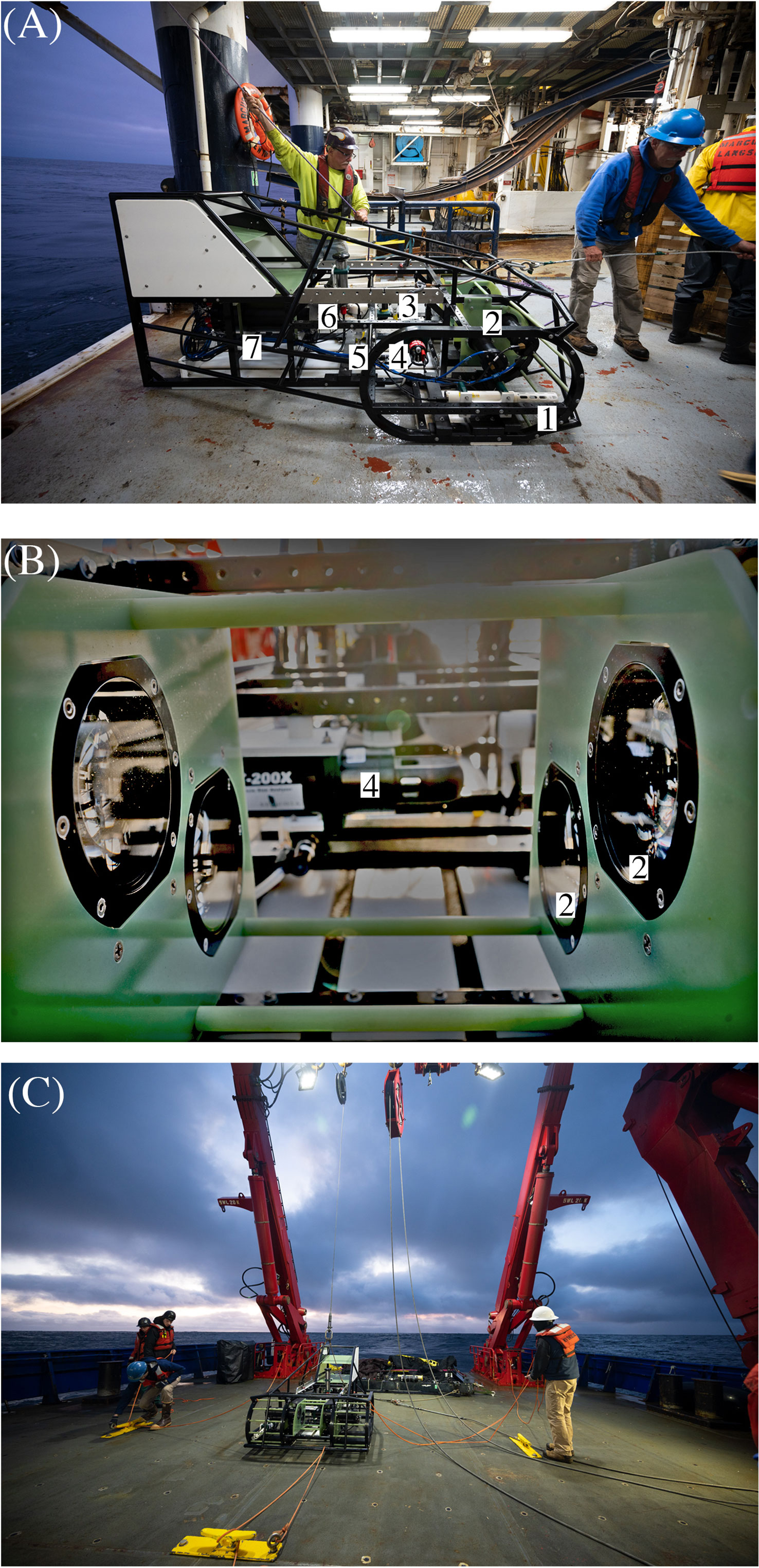
Figure 1 ISIIS-3 and its components (A) Lateral view; 1 = CTD; 2 = two shadowgraph line-scan cameras; 3 = fluorescence and pH sensors as well as altimeter; 4 = LISST-200X particle imager; 5 = pump and dissolved oxygen probe; 6 = flowmeter; 7 = main computer housing. (B) Close-up of the two stacked Bellamare ISIIS-DPI-125 camera units. ISIIS-3 can be deployed through a narrow gate and boom (e.g., on R/V Langseth, A) or via the A-frame (e.g., on R/V Sikuliaq, (C), while side deployments using a crane are also possible and were carried out in the past (e.g., on R/V Atlantis). Photos credit: Ellie Lafferty.

Use of ISIIS and now ISIIS-3 creates a big data challenge. The combination of high-resolution imagery and the need to image a large volume of water results in extremely high numbers of imaged plankton individuals (0.1 to > 1 billion per study; Schmid et al., 2020; Robinson et al., 2021; Schmid et al., 2021; Schmid et al., 2023b). The two line scan cameras of the ISIIS-3 gather 10 GB of data per min, and >35 TB for a typical two-week research cruise (160 h of imagery).

Simultaneous with the development of the ISIIS technology over the last 10 yr., data processing and machine learning pipelines for plankton imagery have also undergone much development (Irisson et al., 2021). Initially, plankton underwater imagery was hand-sorted, but as hard- and software became increasingly available, plankton sorting was automated on desktops with dedicated graphics cards. More recently, university and national supercomputing center machines with enterprise-level graphics cards for machine learning (e.g., NVIDIA A100/V100/P100; Schmid et al., 2021) have become widely available. However, computing time on high-end machines with powerful graphics cards must often be shared with other labs. One solution to this limitation is to tap into nationally funded supercomputing centers, for instance through NSF’s XSEDE infrastructure (now ACCESS; Schmid et al., 2021). XSEDE and ACCESS themselves allocate resources on major national supercomputing centers such as the San Diego Supercomputing Center, or the Pittsburgh Supercomputing Center. While such computing power is critical for analyzing large datasets, they are by necessity ‘post-cruise’ analysis tools, as large node clusters are not portable.

The fact that plankton imagery is usually analyzed after the cruise due to the large quantity of data, precludes it from being used for adaptive sampling, which by definition needs near-immediate data availability. With advancements in ocean technology, thanks to the increased affordability and availability of advanced hard-, and software, the number of studies working on real-time identification and adaptive sampling based on different underwater vehicles has increased though in recent years (Fossum et al., 2019; Ohman et al., 2019; Stankiewicz et al., 2021; Bi et al., 2022). However, having the necessary computing power at sea to classify large quantities of videography remains a bottleneck.

Recent increased availability of edge servers in the civilian sector may resolve this bottleneck, enabling oceanographers to take significant computing power to sea with the potential to acquire and analyze extensive data sets while at sea and even during active deployments. In the case of plankton imaging, edge servers coupled with deep-learning pipelines, enable researchers to not only store and back-up the data on redundant drives, but to process the incoming videography (i.e., segmentation and classification), and analyze the data for distributional patterns, all while the instrument is being towed behind the ship. These combined technologies enable the scientific sampling plan to change based on real-time information gathered at-sea. This approach has major consequences for the way oceanographic research can be conducted as it makes adaptive sampling possible - meaning that oceanographic features of interest, e.g., accumulations of particular taxa in low or even hypoxic oxygen waters on the NCC shelf (Chan et al., 2008; Chan et al., 2019), can be targeted for resampling immediately after their detection. A separate benefit of processing data at sea is the ability to reduce (or completely remove) the lag between scientific research cruise completion and being able to work with data for ecological analyses. Here we describe a deep learning pipeline for plankton classification at sea, including databasing and visualization for adaptive sampling. We describe the necessary hardware setup for such an adaptive sampling processing pipeline and how it could be adapted for other imaging systems. The major deliverable is the open-sourced code for the pipeline including classification as well as automation scripts for databasing and visualization. At-sea processing of complex data has the potential to transform oceanographic science.

2 Materials and equipment

2.1 In-situ ichthyoplankton imaging system-3

The In-situ Ichthyoplankton Imaging System (ISIIS) vehicle has undergone several design modifications since its early inception (Cowen and Guigand, 2008). Here we report on the third vehicle iteration or model - the ISIIS-3. ISIIS-3 (Figure 1) was developed based on several lessons learned from the original design, including a robust open-frame sled design and dual tow point bridle that promotes the shedding of buoyed markers of active fishing gear (e.g., crab pots). The system includes a dual camera setup (55 μm pixel resolution) instead of a single camera to enable a narrower sled design, but without compromising the total sampling volume of 180 L s^-1. The system is also more modular than the ISIIS-1 and ISIIS-2 towed vehicles, enabling easier integration of new electronic components. For instance, ISIIS-3 is fitted with a Sequoia Scientific LISST-200X particle imager covering the 1 μm - 500 μm size range, a CTD (Sea-Bird SBE 49 FastCAT), dissolved oxygen probe (Sea-Bird 43), fluorescence sensor (Wet Labs FLRT), photosynthetically active radiation sensor (PAR; Biospherical QCP-2300), and a pH sensor (Seabird SBE 18). ISIIS-3 is towed behind the ship at 2.5 m s^-1 where it undulates typically between 1 m and 100 m depth or as close as 2 m above the seafloor in shallower waters on the shelf. Data are continuously multiplexed in the ISIIS-3 vehicle, and then sent to the ISIIS-3 control computer on the ship through the glass-fiber of the oceanographic wire, where data are then de-multiplexed and time-stamped.

2.2 Edge server configuration at sea

The edge server used here was a Western Digital (WD) Ultrastar-Edge MR with two Intel Xeon Gold 6230T 2.1 GHz CPUs, each with 20 cores (40 cores total), a NVIDIA Tesla T4 GPU, 512 GiB DDR4 memory, >60 TB of NVMe flash storage, as well as 100 GbE and 10 GbE networking (Figure 2). The edge server ran with Ubuntu 20.04 and DNS, DHCP, TFTP, and HTTP services, enabling the setup of an intranet around the edge server. The NVMe file space of the edge server was configured into a RAID to allow for limited redundancy; specifically, we use ZFS cut with RAIDZ2 with no spares. This provided around 40 TB of usable space and allowed failure of a drive without having to rebuild the drive during data collection. Rebuilding a drive during live data collection would slow down write speed substantially and potentially lead to a loss of image frames.

FIGURE 2

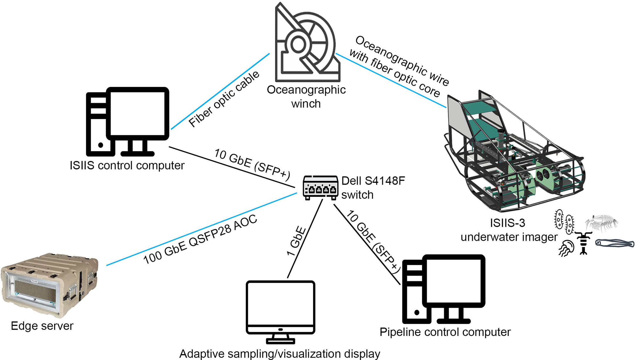
Figure 2 The hardware setup associated with the ISIIS-3 control computer and edge server. ISIIS-3 is connected to the ISIIS-3 control computer via fiber (all optic connections in blue). Incoming data are used for flying the sled (e.g., using depth information, altimeter, and speed through the water) and incoming imagery and environmental sensor data are time-stamped and deposited directly on the edge server. While the connection from ISIIS-3 control computer to the switch is rated at 10 GbE, the connection from the switch to the edge server is a 100 GbE active optics cable (AOC) to allow for additional I/O for running the pipeline, offloading data, and sending data to the visualization display.

The DHCP on the edge server enabled other machines on the network (switch and VLAN) to be serviced by the edge server (Figure 2). This allowed us to deploy a Dell S4148F switch with 10 GbE, 40 GbE and 100 GbE ports to support a large range of devices that needed to be connected to the edge server. SFP+ to RJ45 transceiver modules were used to allow laptops and other devices to connect to the isolated network. The DHCP server was configured to have known hosts with fixed addresses to best support services that relied on being on the same IP upon reboots. SAMBA services were used to allow the ISIIS-3 control computer (running Windows 10) to directly save incoming video data to the edge server. An additional Ubuntu 20.04 desktop was used to control the processing pipeline on the edge server through SSH, and a MacOSX desktop was used for running the webserver that visualized real-time classified plankton information (e.g., length of segmented particles and plankton as well as taxonomic identity), using the Python API 2.0 HeavyDB interface (Schmid et al., 2023a; see reference to heavyDB). A 10-m 100 GbE QSFP28 AOC cable allowed the set-up of the edge server in a separate temperature-controlled server room on the ship, removing the edge server fan noise from the science labs while retaining an extremely fast connection and leaving enough I/O for simultaneous writing of incoming imagery, data offload, pipeline control, and sending of data to a database. The ISIIS-3 control computer only supported a 10GbE network card, but over the SAMBA mounts the ISIIS-3 control computer was able to write to the edge server at ~400MB/s, about twice the throughput that was needed for the raw imagery, leaving plenty of I/O on the drives of the edge server to simultaneously process data.

3 Methods

3.1 Image processing pipeline

The image processing pipeline controller scripts are primarily written in Python 3 and call binaries that need to be compiled first (Figure 3). Segmentation (https://github.com/paradom/Threshold-MSER/tree/spectra-dev) and classification binaries are provided in the zenodo pipeline repository for this paper (http://dx.doi.org/10.5281/zenodo.7739010). Incoming video files are automatically ingested into the image processing pipeline by the automate.py script monitoring the incoming data folder (Figure 3). Incoming AVI files are segmented via threshold-MSER (T-MSER; Panaïotis et al., 2022) using the CPU cores of the edge server (Figure 3). T-MSER is optimized for multithreading and general speed due to the volume of data generated by the two ISIIS-Deep Particle Imager (DPI) cameras. Multithreading of segmentation and classification is controlled by the OpenMP Python library and based on available resources. On the edge server with 40 cores, 20 processes can be run in parallel. After the flat-fielding of individual frames, T-MSER uses a signal-to-noise ratio (SNR) switch, after which low noise frames are directly segmented using Maximally Stable Extremal Regions (MSER, Matas et al., 2004; Bi et al., 2015; Cheng et al., 2019), and high noise frames are first pre-processed with a thresholding approach before applying MSER. T-MSER was written in C++. The lower size cutoff for the segmentation, determining which size segments (i.e., plankton) are retained, can be set to the desired value based on the study’s objectives; here we used 49 pixels of object area as the lower size cutoff for retention of segments.

FIGURE 3

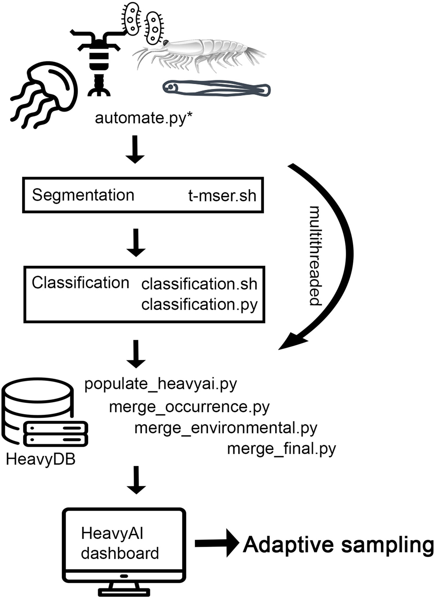
Figure 3 Pipeline schematic depicting the imagery data processing pipeline deployed at sea. The automate.py script controls all subsequent processes, including ingestion of imagery into segmentation and classification, merging of the different data products, and upload into HeavyDB. The HeavyAI dashboard monitors the HeavyDB and visualizes new data (e.g., depth stratified plankton identifications) as they become available. The dynamic and interlinked figures in the dashboard are then used for adaptive sampling. Flowchart text with file extensions depicts all the files necessary to run the pipeline, which can be found in the online repository. Text without file extensions describes larger concepts and gives context.

As soon as AVIs are segmented automate.py starts the classification process on these segments using a sparse Convolutional Neural Net (sCNN, Graham et al., 2015; Luo et al., 2018; Schmid et al., 2021). The edge server’s NVIDIA T4 GPU (Figure 3) supported four classification processes running in parallel. The sCNN was previously trained on an image library containing 170 classes of particles and plankton from the NCC, until the error rate of the classifier plateaued at ~ 5% after 399 epochs. After applying the classifier to new imagery, a random subset of images was classified by two human annotators and compared with the automated identifications to create a confusion matrix. Based on the confusion matrix information (e.g., false positives and true positives) and the known underlying assigned probabilities per image given by the sCNN, we used probability filtering (Faillettaz et al., 2016) to remove very low probability images from the dataset that lead to false positives and false negatives. Using LOESS modeling, we established at which assigned probability a cutoff had to be made to achieving 90% predictive accuracy for the taxon. Removal of these low‐confidence images retains true spatial distributions (Faillettaz et al., 2016). The process and accuracies are described in more detail in previously published work (Briseño-Avena et al., 2020b; Schmid et al., 2020; Swieca et al., 2020; Schmid et al., 2021; Greer et al., 2023; Schmid et al., 2023b). The pipeline described here is open-sourced at: http://dx.doi.org/10.5281/zenodo.7739010.

3.2 Database and webserver visualization

Ship data (e.g., GPS feed), ISIIS-3 environmental sensor data (e.g., pH, dissolved oxygen), plankton size measurements, and classification probabilities are merged based on microsecond-accurate timestamps by the populate_heavyai.py script and its subroutines (Figure 3). The same script also uploads merged data into the HeavyDB database as soon as they become available. A heavy.ai dashboard that is linked to HeavyDB can then visualize the data in an immersive way, enabling data interpretation and adaptive sampling.

4 Results

4.1 At-sea processing with the edge server

In July 2022, ISIIS-3 was towed along six transects off the WA and OR coasts with each transect ranging from 8 to 14 h long. During these tows, ISIIS-3 imaged plankton ranging from small phytoplankton and protists, to crustaceans, gelatinous plankton such as salps and appendicularians, and larval fishes. These organisms spanned a large size range and differed significantly in their body form (e.g., fragile gelatinous plankton vs hard-shelled crustaceans, Figure 4). By imaging these different organisms in a non-invasive way, we obtained data on their overall distribution and abundance across multiple scales, as well as insights into their natural behaviors and orientations in the water column and potential predators-prey relationships (Ohman, 2019). Along the six transects, 36 TB of data were collected from the two ISIIS-DPI cameras, totaling over 120 h of imagery (60 h per camera).

FIGURE 4

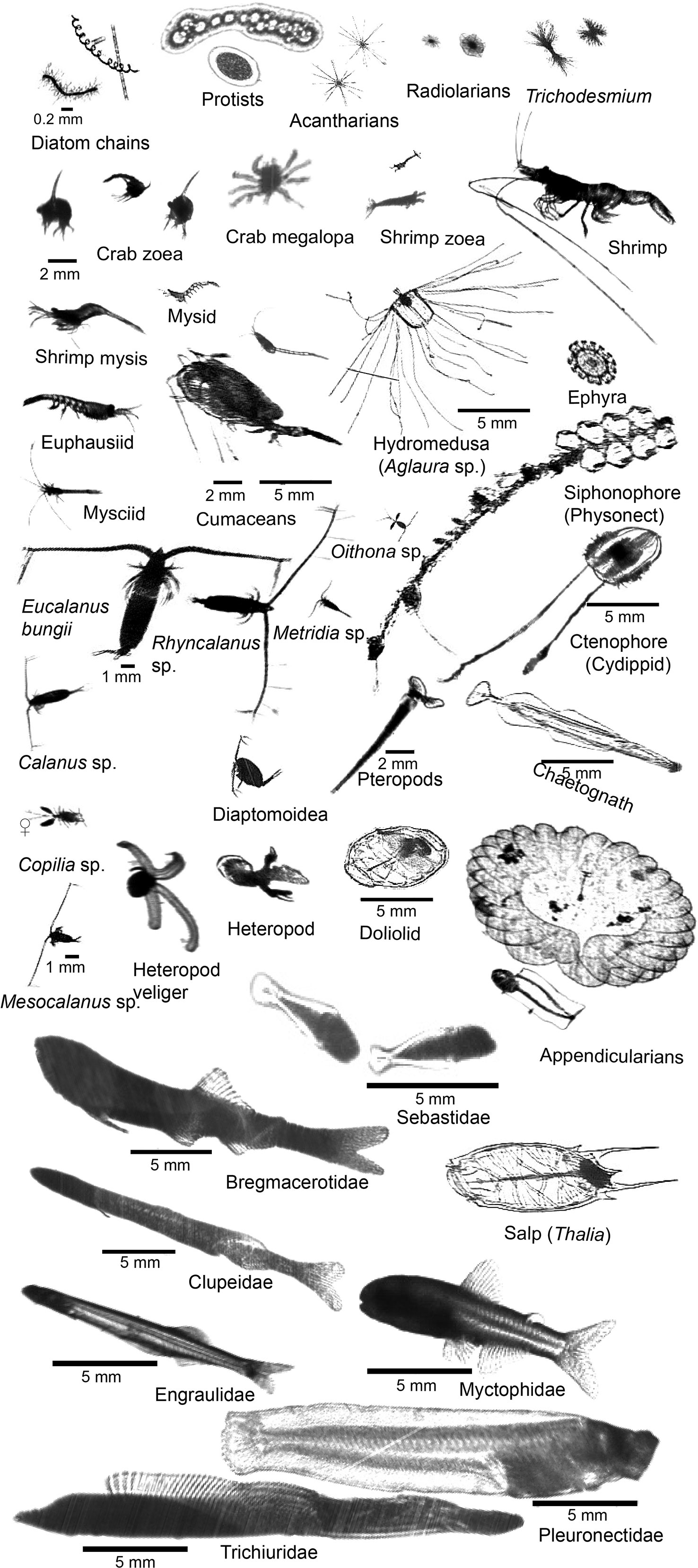
Figure 4 ISIIS-DPI images of key taxa in the Northern California Current including primary producers, protists, crustaceans, cnidarians, ctenophores, echinoderms, heteropods, pteropods, chaetognaths, pelagic tunicates, and larval fishes.

T-MSER segmentation on the edge server’s 40 CPUs took 1.1 mins per 50 sec of video data, while classification on the T4 GPUs took an additional 2.65 mins on average, bringing the total time lag between data collection and having classified results to 3.75 mins. The speed of the pipeline becomes even more apparent when taking into account that an AVI contains between 23,000 and 225,000 segments of particles and organisms, depending on the biological productivity (Panaïotis et al., 2022). Especially dense phytoplankton layers led to longer segmentation and classification times. With that in mind, segmentation and classification together can take between 2.5 - 5 min per 50 sec AVI.

4.2 Database and visualization of plankton classifications for adaptive sampling

The HeavyDB database updated automatically as new data were classified, and included the taxonomic identifications and lengths of each detected object together with their environmental data (e.g., pH, oxygen), as well as GPS location from ship sensors. Database and heavy.ai dashboard were very responsive, running on the edge server’s 512 GB memory and the NVMe flash storage. Hence, visualization of data on the heavy.ai dashboard was smooth and updated quickly based on the user selections (Figure 5). The dashboard can be customized by the user to show different data presentations. Shown here are standard features – number of classified images used in the data presentation, number of unique taxa classified, allocation of classified images across taxa, sampling location, as well as location specific sampling depth (note, in this case, our transect ran east-west along a constant latitude). The user can select which taxa (or all) to display – in this example, we show the vertical distribution (in 2-m depth bins) of all taxa combined. We also show the size spectrum of all classified segments across 76 bins of major axis segmented image size (i.e., based on number of pixels). Other data presentations can easily be developed by the user by clicking “add chart” on the dashboard. Data presentation is updated continually as new classifications are completed. Heavy.ai dashboard graphics are dynamic and interlinked so that selection of a taxon, size range, or time interval, leads to all other plots defaulting to that sub-selection. For instance, selection of Oithona sp. copepods in the taxa overview leads to the size spectrum and 3-D vertical distribution plots showing only data of Oithona sp. copepods. Multiple simultaneous selections are possible and a powerful and intuitive tool for adaptive sampling.

FIGURE 5

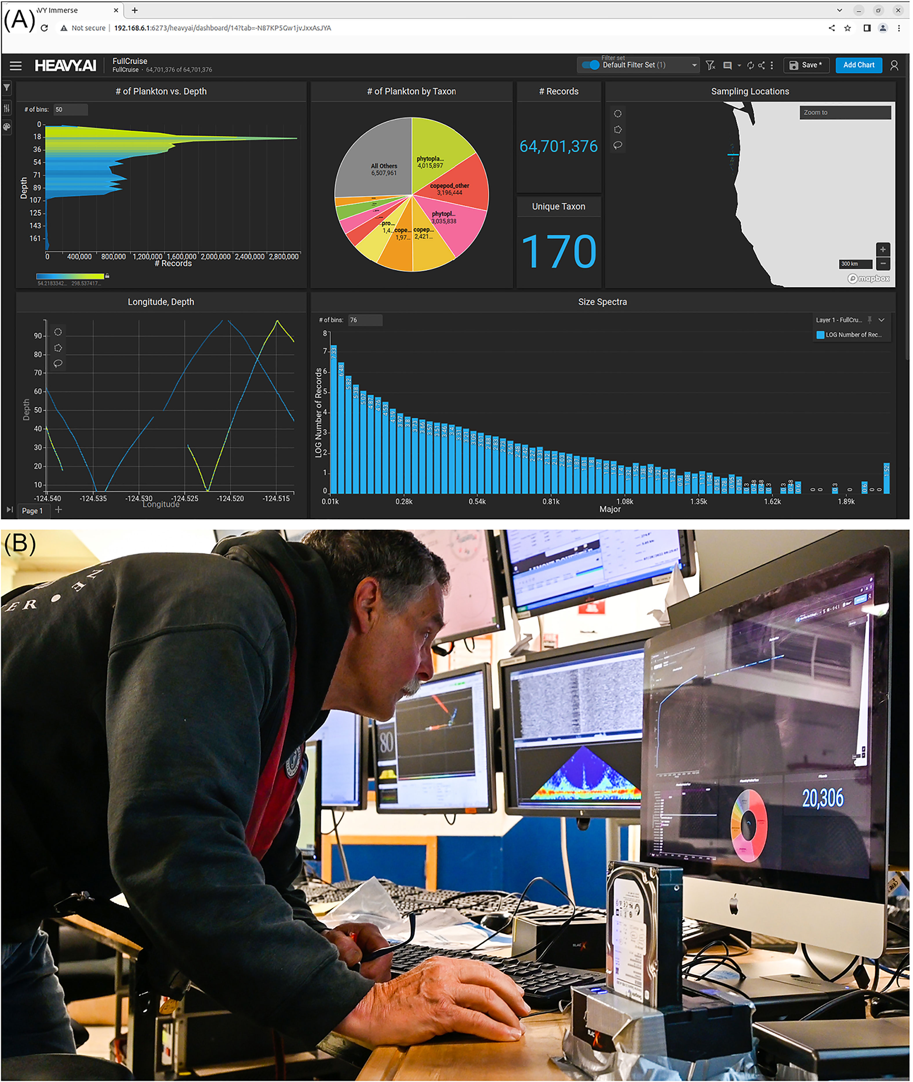
Figure 5 (A) The HeavyAI dashboard displayed on the adaptive sampling display. The user can add and delete different figure types. Clockwise from the upper left, are: the vertical distribution of plankton counts in the water column, the relative abundance of taxa (as a pie chart), the geolocation of samples (map), the size distribution of plankton taxa (histogram), and the vertical distribution of plankton taxa with longitude. Selecting a swath of vertical distribution or a specific taxon in the pie chart automatically adapts all other figures to the sub-selection, for instance only showing a certain taxon – multiple sub-selections at the same time are possible (e.g., adapting all figures to only show Oithona sp. copepods in the top 20 meters that have a certain size). The HeavyAI dashboard monitors the underlying HeavyDB for new incoming data to display. (B) This setup lends itself to near real-time data exploration and adaptive sampling.

5 Discussion

Using the edge server for live classification of plankton imagery yielded bountiful data for exploration during the cruise and for adaptive sampling. Use cases for adaptive sampling in biological oceanography that have the potential to transform oceanography include on-the-fly and fast detection of species of interest, detection and resampling of thin layer associated organisms, as well as high spatial resolution adaptive sampling of taxa present in, or at the interface of, environmental features of high importance such as low oxygen zones on the NCC shelf.

5.1 Example applications for adaptive sampling

Access to real-time or near real-time taxon-specific distribution and abundance data is novel in most oceanographic studies, particularly access to very detailed spatial and vertical resolution. With such data in hand, while at sea, the researcher can be responsive to short-lived events (e.g., thin layers, sub-mesoscale eddies, other aggregative features), to specific taxa that might be ephemeral or highly patchy, and to environmental conditions that are of particular interest (e.g., low oxygen). With the ability to identify such features or taxa of interest while still at sea, the researcher can adapt their sampling to a more specific target. Below are several examples where sampling could be adapted in response to the detection of specific features or events.

5.1.1 Vertical migration

Diurnal vertical migration (DVM) is a well-known, but often challenging process to adequately sample biologically. Acoustic echograms can help visualize the movement of reflective organisms, but actual species composition of the observed acoustic signal requires in situ sampling. While a plankton net might be able to verify the dominant species present in such a feature, it will not provide detailed vertical distribution data of different species. Fine spatial separation may occur under some scenarios as different species may swim/rise at different speeds, and determination, let alone verification of that pattern is difficult at best with only acoustic data (Figure 6). Towing an imaging system such as ISIIS-3 with near-real time data output, can enable a detailed biological survey of the feature, even as it is rising or falling in the water column.

FIGURE 6

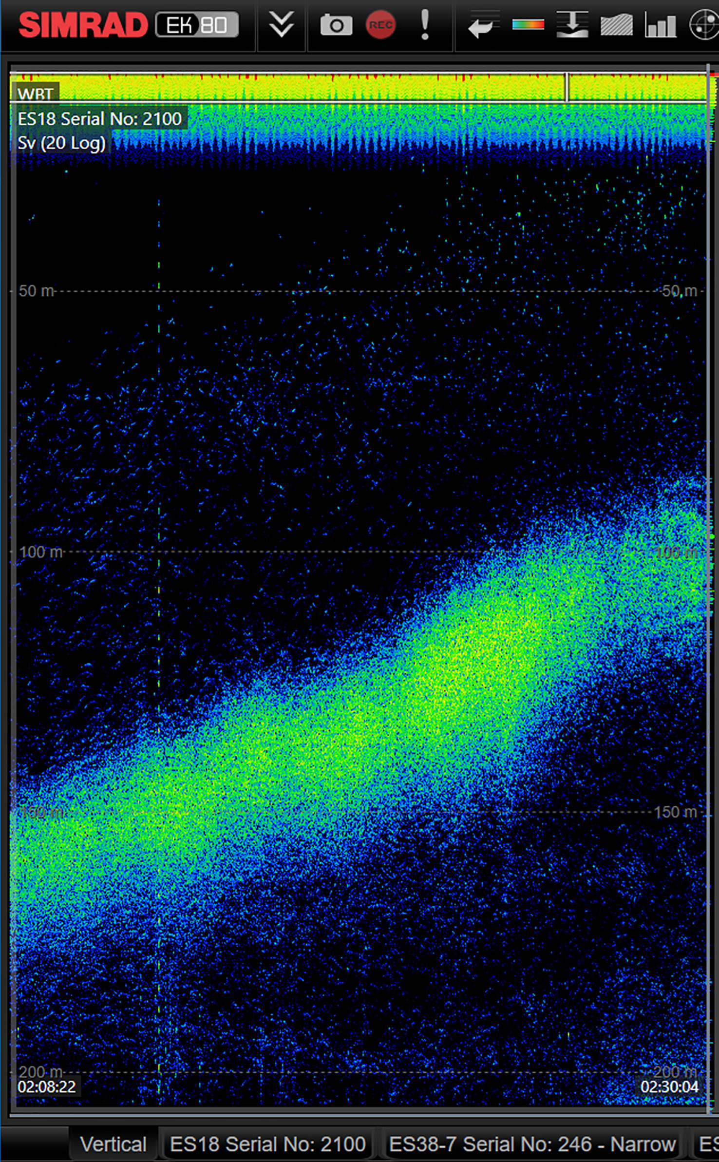
Figure 6 A snapshot from the EK80 18 kHz backscatter signal showing evidence of plankton diel vertical migration to surface waters during early evening hours. Time is on the x-axis, depth on the y-axis. Combining live observations from the EK80 with live ISIIS-DPI imagery and the heavyAI dashboard enables a new way of adaptive sampling by being able to pinpoint the taxa comprising such diel migration patterns.

5.1.2 Thin layers and other patchy features

Algal thin layers are often highly transient in location and persistence. While their presence may be predictable in some situations (e.g., Greer et al., 2013; Greer et al., 2020; McManus et al., 2021), actual encounter of them may be a chance occurrence, and indication of their presence may be vague (e.g., Chl a signal appearing highly noisy). Verifying the presence, and detailing the vertical distribution of organisms associated with a thin layer can only be done with focused vertical sampling. Real-time high resolution imagery data can more accurately verify the presence of a thin layer and its various species constituents, and then can be utilized in developing an adaptive sampling plan to more fully resolve the dimensions and species interactions associated with the thin layer.

Vertically and spatially discrete aggregations of other organisms are not uncommon (Robinson et al., 2021), though difficult to predict. Their presence may be associated with a specific life stage, or in response to certain biological or physical features and their relative importance (i.e., as a predator or prey source) may depend on the extent of the patch (or bloom). For example, small patches of dense hydromedusae aggregations (Figure 7), which can exert substantial predation pressure on larval fishes and copepods (Corrales-Ugalde and Sutherland, 2021; Corrales-Ugalde et al., 2021), are difficult to sample with nets. As with other aggregations, when hydromedusae are identified though in-situ imaging and real-time AI at sea, researchers have the potential to adjust sampling efforts to resolve the dimensions and density of patches.

FIGURE 7

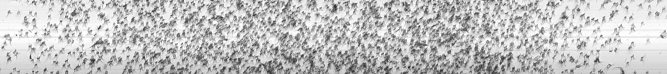
Figure 7 A snapshot of ISIIS-DPI imagery as the sled is towed along a transect in the southern California Current. Dense patches of organisms, in this case hydromedusae, can be observed and re-sampled to identify the extent of patches and layers. Using near real-time classification with an edge server enables the identification and quantification of dense patches. The layer shown here spans 1.17 m from edge to edge.

5.1.3 Specific environmental conditions of high interest

As with focused sampling around biological aggregations, adaptive sampling around specific oceanographic conditions can reveal novel biological patterns and associations. Follow-up sampling at various physical interfaces, as identified by other sensors, might reveal changes in organism distributions warranting further study. For example, vertical or horizontal frontal features detected by Acoustic Doppler Current Profilers (ADCP; Figure 8), might suggest broad, then more fine-tuned sampling as real-time data analyses reveal spatial biological patterns. Eddie fronts (potentially detected by ADCP) are prime examples for where adaptive re-sampling of the eddy’s interface could provide valuable insight into the taxonomic make-up of eddy, interface, and exterior water masses (Schmid et al., 2020).

FIGURE 8

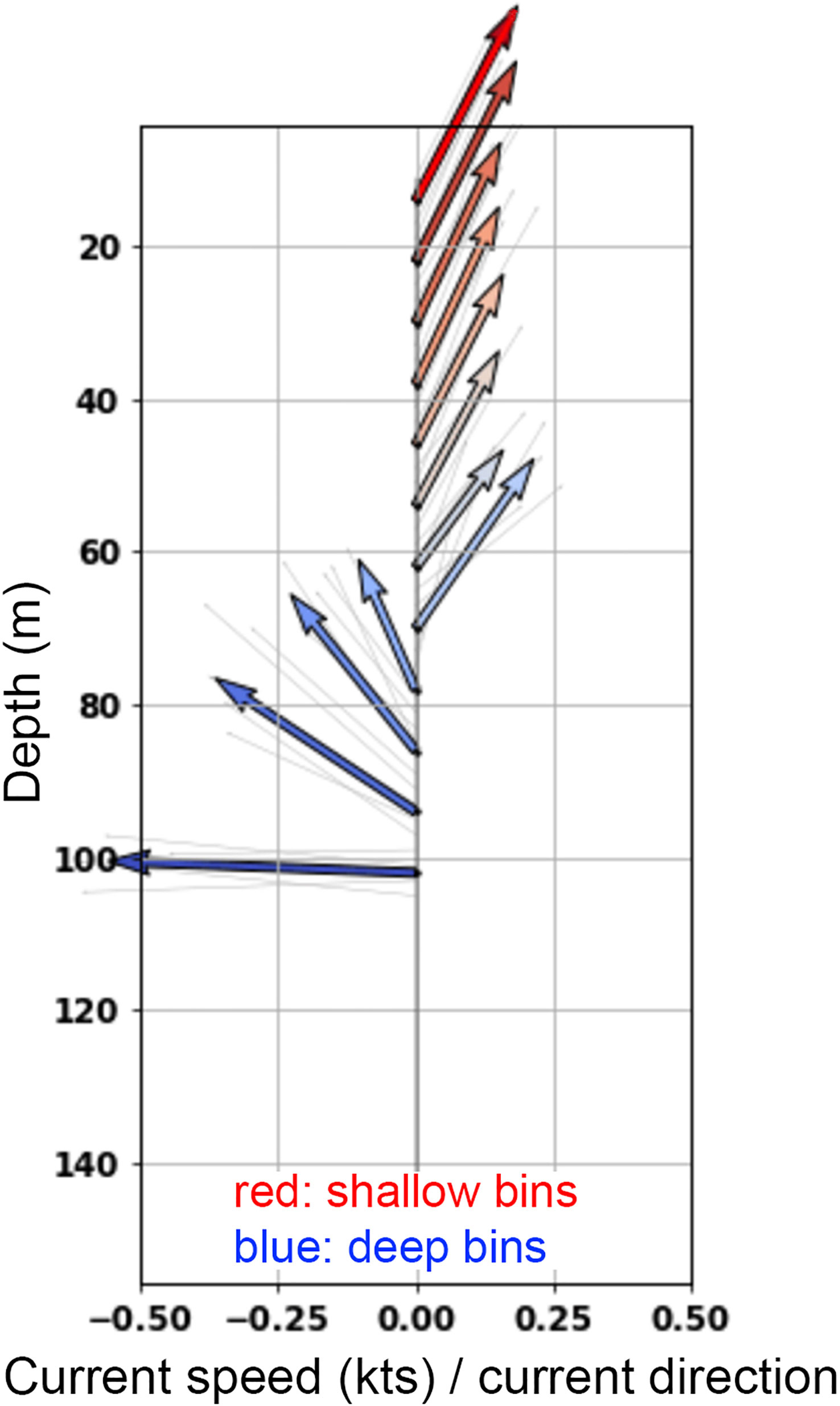
Figure 8 A snapshot of an ADCP vector diagram as seen on the real-time readout on research vessels. Using real time classification of encountered plankton in conjunction with ADCP data allows the immediate re-sampling of ocean conditions of high importance, such as vertical and horizontal fronts. In this ADCP vector diagram, surface waters (5-60 m) are characterized by distinct northeastward flow, while at depths below 75 m water is moving in a northwest to west direction. Using readouts from the heavyAI dashboard, the ISIIS-3 imager can be towed specifically at the interface of such divergent flows in order to collect the most insightful data on taxa distributions, potential predator-prey interactions facilitated by such features, as well as behavioral observations. The y-axis shows depth; however, each arrow has a directional and speed component. Colors are not quantitative but indicate shallow and deep bins. The direction of the arrows indicates 360 deg direction, with arrows upward indicating “North”.

Finally, coupling physical and optical sensors can enhance adaptive sampling capability. On the NCC shelf, in particular, low oxygen upwelled water can quickly become further hypoxic when primary productivity decays after phytoplankton blooms (Chan et al., 2008). Such low oxygen zones are increasing in frequency and duration and have become an emerging threat to fisheries (Chan et al., 2008; Chan et al., 2019) that can lead to substantial financial loss. Sensors on imaging systems can detect such low oxygen zones (Figure 9) and using the imager, these low oxygen waters can be re-sampled on transects passing from normoxic waters, through the interface, and into the core of hypoxic waters. Near-real-time processing can detect the expected and unexpected presence of different taxa, which can lead to new insights and hypotheses. For example, in 2016, anchovy larvae were imaged in low oxygen waters (Briseño-Avena et al., 2020b) on the Newport Hydrographic Line, a transect sampled since 1961 (Peterson and Miller, 1975).

FIGURE 9

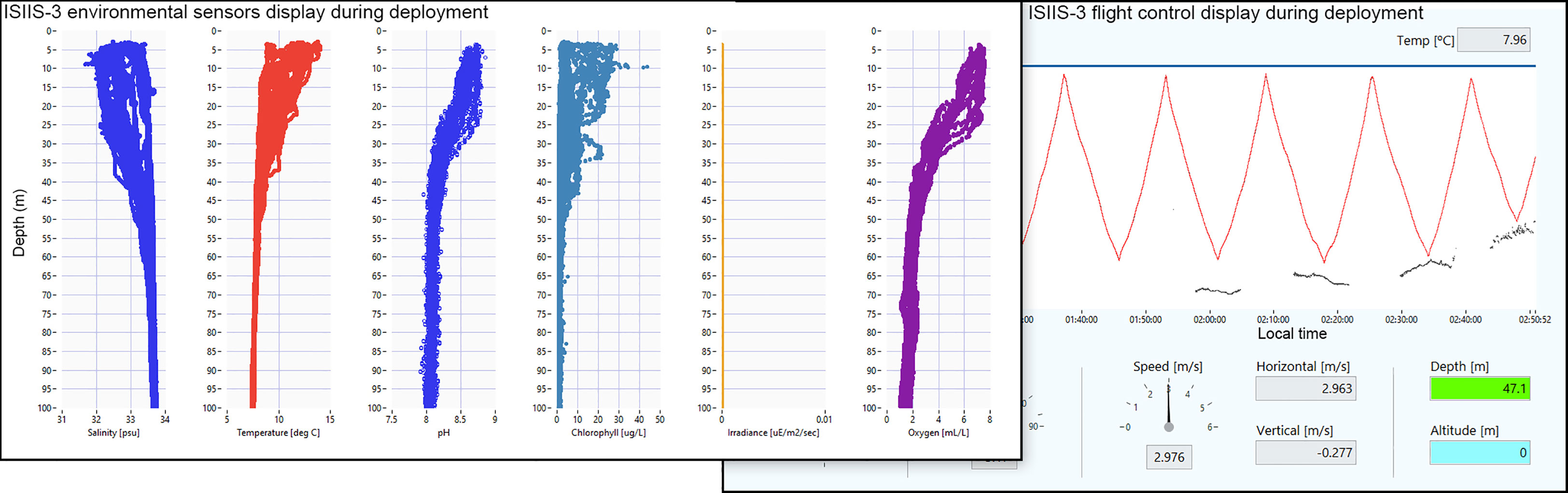
Figure 9 ISIIS-3 control display during a transect on the Heceta Head line (43.98° N) off Oregon, with environmental data plotted on the left (e.g., dissolved Oxygen as low as < 1 ml L^-1 at 100 m depth). The right panel shows the undulating flight pattern (red line) and demonstrates ISIIS-3’s ability to sample hypoxic waters at near bottom depths (blue points are the seafloor as indicated by the altimeter).

In combination, the examples presented here are a considerable advancement in our ability to find, identify, and thoroughly sample ephemeral and other hard-to-detect features in the ocean. Adaptive sampling using cutting edge technology is critical to expand our understanding of the processes that are driving ocean biology.

5.2 Processing speeds

The edge server’s NVMe flash drives and CPU succeeded in segmenting the incoming.avi video files almost at 1:1 ratio of collection time vs processing time. A single NVIDIA T4 GPU with 16 GB memory was able to classify data in four parallel instances, adding on average another 2.65 mins for classification of each AVI. While the achieved processing times were good and within our expectations, we envision more powerful hardware in conjunction with even more specialized software to segment incoming AVIs at a ratio of 1:0.5 or faster – and cutting down on classification time in a similar way, in order to go from near real-time processing and display of data to real-time classification and display. Depending on the detected oceanographic features or a priori features the user wants to investigate with regards to the distribution of taxa, the ability to see which taxa are present with a 1 min time lag vs a 5 mins time lag, likely makes a big difference.

5.3 Implementing the adaptive sampling pipeline with other imaging system setups and edge servers

The pipeline code and workflow described here were designed with the idea of being agnostic to the imaging system used as well as the specific edge server available. For instance, while our specific setup receives large quantities of data through a fiber optic cable that are then ingested into the pipeline on the edge server, this is by no means a necessary pathway. The output of any imaging system could be used with this setup by similarly creating network drives on the imaging system’s data collection computer, pointing to the edge server for writing files and immediate processing – how the imagery gets to the edge server is of little importance as long as the time lag between collecting the data and starting to process is minimized. This also means that while the presented pipeline is targeting live data-feed imaging systems, one could easily take the setup described here and supply data from profilers that do not transmit data live (e.g., the Underwater Vision Profiler 6), as soon as the data from a profile is retrieved. In that context, a user can also replace the segmentation and classification described here with an instant segmentation approach such as the You Only Look Once (YOLO; Jiang et al., 2022) algorithm or similar. The idea of an edge server is to have powerful hardware (i.e., CPU, GPU, memory, storage) in a relatively low power consumption package that has a small footprint and is ruggedized. There are a diversity of edge servers available on the market that can be bought or home-built and that could be used instead of the one used here. When switching to a GPU-based YOLO or Mask R-CNN (He et al., 2017) object detection, the user would be less reliant on CPUs and thus might prefer a setup with fewer CPUs while swapping in several more powerful GPUs instead.

5.4 Conclusion

ISIIS-3 in conjunction with a deep learning pipeline deployed on an edge server at sea is a powerful combination for adaptive sampling, reducing lag between data collection and addressing on ecological questions, as well as for scientific discussions with cruise participants. Several applications of adaptive sampling were presented that have the potential to be transformative for oceanographic research, including in-situ target species identification, and HAB thin layer characterization. In the northern California Current, where hypoxia and ocean acidification are endangering commercially important taxa such as Dungeness crab and hence the livelihood of communities, adaptive sampling of taxa distributions in such features could prove a very effective tool for better understanding the responses of such taxa to environmental disturbances.

Data availability statement

The datasets presented in this study can be found in the online repositories below: Processing pipeline open-sourced at: http://dx.doi.org/10.5281/zenodo.7739010; NSF’s BCO-DMO: https://www.bco-dmo.org/project/855248; R2R program: https://www.rvdata.us/search/vessel/Langseth.

Ethics statement

The animal study was reviewed and approved by Oregon State University’s Institutional Animal Care and Use Committee (IACUC). Written informed consent was obtained from the individual(s) for the publication of any potentially identifiable images or data included in this article.

Author contributions

MS performed analyses and wrote the initial manuscript; MS, CS, SS, and RC conceptualized hypotheses and research questions; DD, MD, and CS wrote and deployed pipeline code on the edge server, MS and CS supervised pipeline development; MS, SS, and RC wrote grant proposals; MS, DD, and RC collected data; CG, CC, MS, and RC designed ISIIS-3, CG and CC were responsible for ISIIS-3 engineering. All authors contributed to the article and approved the submitted version.

Funding

Support for this study was provided by NSF OCE-1737399, NSF OCE-2125407, NSF RISE-1927710, and NSF XSEDE/ACCESS OCE170012.

Acknowledgments

We thank current and former Oregon State University, Hatfield Marine Science Center, Plankton Ecology Lab members who helped collect ISIIS-3 data during the R/V Langseth cruise: Elena Conser, Luke Bobay, Jami Ivory, and Megan Wilson. Jassem Shahrani from Sixclear Inc coded the ISIIS-3 control software using the JADE application development environment and was very helpful whenever questions came up. Sergiu Sanielevici and Roberto Gomez from the Pittsburgh Supercomputing Center were instrumental in the development of previous iterations of the pipeline, which later allowed successful porting of components to the edge server. We thank David A. Jarvis at Western Digital for working with us and providing access to the edge server.

Conflict of interest

The authors declare that the research was conducted in the absence of any commercial or financial relationships that could be construed as a potential conflict of interest.

The authors declare that the edge server was donated to Oregon State University by Western Digital, and that the results presented here are in no way influenced by this donation. ISIIS-3 was procured from Bellamare LLC. No other commercial or financial relationships that could be construed as a potential conflict of interest are present.

Publisher’s note

All claims expressed in this article are solely those of the authors and do not necessarily represent those of their affiliated organizations, or those of the publisher, the editors and the reviewers. Any product that may be evaluated in this article, or claim that may be made by its manufacturer, is not guaranteed or endorsed by the publisher.

References

Bi H., Guo Z., Benfield M. C., Fan C., Ford M., Shahrestani S., et al. (2015). A semi-automated image analysis procedure for In situ plankton imaging systems. PloS One 10, e0127121. doi: 10.1371/journal.pone.0127121

PubMed Abstract | CrossRef Full Text | Google Scholar

Bi H., Song J., Zhao J., Liu H., Cheng X., Wang L., et al. (2022). Temporal characteristics of plankton indicators in coastal waters: high-frequency data from PlanktonScope. J. Sea Res. 189, 102283. doi: 10.1016/j.seares.2022.102283

CrossRef Full Text | Google Scholar

Briseño-Avena C., Prairie J. C., Franks P. J. S., Jaffe J. S. (2020a). Comparing vertical distributions of chl-a fluorescence, marine snow, and taxon-specific zooplankton in relation to density using high-resolution optical measurements. Front. Mar. Sci. 7. doi: 10.3389/fmars.2020.00602

CrossRef Full Text | Google Scholar

Briseño-Avena C., Schmid M. S., Swieca K., Sponaugle S., Brodeur R. D., Cowen R. K. (2020b). Three-dimensional cross-shelf zooplankton distributions off the central Oregon coast during anomalous oceanographic conditions. Prog. Oceanogr. 188, 102436. doi: 10.1016/j.pocean.2020.102436

CrossRef Full Text | Google Scholar

Chan F., Barth J., Kroeker K., Lubchenco J., Menge B. (2019). The dynamics and impact of ocean acidification and hypoxia: insights from sustained investigations in the northern California current Large marine ecosystem. Oceanography 32, 62–71. doi: 10.5670/oceanog.2019.312

CrossRef Full Text | Google Scholar

Chan F., Barth J. A., Lubchenco J., Kirincich A., Weeks H., Peterson W. T., et al. (2008). Emergence of anoxia in the California current Large marine ecosystem. Science 319, 920–920. doi: 10.1126/science.1149016

PubMed Abstract | CrossRef Full Text | Google Scholar

Cheng K., Cheng X., Wang Y., Bi H., Benfield M. C. (2019). Enhanced convolutional neural network for plankton identification and enumeration. PloS One 14, e0219570. doi: 10.1371/journal.pone.0219570

PubMed Abstract | CrossRef Full Text | Google Scholar

Corrales-Ugalde M., Sponaugle S., Cowen R. K., Sutherland K. R. (2021). Seasonal hydromedusan feeding patterns in an Eastern boundary current show consistent predation on primary consumers. J. Plankton Res. 43, 712–724. doi: 10.1093/plankt/fbab059

CrossRef Full Text | Google Scholar

Corrales-Ugalde M., Sutherland K. R. (2021). Fluid mechanics of feeding determine the trophic niche of the hydromedusa clytia gregaria. Limnol. Oceanogr. 66, 939–953. doi: 10.1002/lno.11653

CrossRef Full Text | Google Scholar

Cowen R. K., Guigand C. M. (2008). In situ ichthyoplankton imaging system (ISIIS): system design and preliminary results. Limnol. Oceanogr. Methods 6, 126–132. doi: 10.4319/lom.2008.6.126

CrossRef Full Text | Google Scholar

Faillettaz R., Picheral M., Luo J. Y., Guigand C., Cowen R. K., Irisson J.-O. (2016). Imperfect automatic image classification successfully describes plankton distribution patterns. Methods Oceanogr. 15, 60–77. doi: 10.1016/j.mio.2016.04.003

CrossRef Full Text | Google Scholar

Fossum T. O., Fragoso G. M., Davies E. J., Ullgren J. E., Mendes R., Johnsen G., et al. (2019). Toward adaptive robotic sampling of phytoplankton in the coastal ocean. Sci. Robotics 4, eaav3041. doi: 10.1126/scirobotics.aav3041

CrossRef Full Text | Google Scholar

Graham B. (2015). Fractional max-pooling. Arxiv 1–10. doi: 10.48550/arxiv.1412.6071

CrossRef Full Text | Google Scholar

Greer A. T., Boyette A. D., Cruz V. J., Cambazoglu M. K., Dzwonkowski B., Chiaverano L. M., et al. (2020). Contrasting fine-scale distributional patterns of zooplankton driven by the formation of a diatom-dominated thin layer. Limnol. Oceanogr. 65, 2236–2258. doi: 10.1002/lno.11450

CrossRef Full Text | Google Scholar

Greer A. T., Cowen R. K., Guigand C. M., McManus M. A., Sevadjian J. C., Timmerman A. H. V. (2013). Relationships between phytoplankton thin layers and the fine-scale vertical distributions of two trophic levels of zooplankton. J. Plankton Res. 35, 939–956. doi: 10.1093/plankt/fbt056

CrossRef Full Text | Google Scholar

Greer A. T., Schmid M. S., Duffy P. I., Robinson K. L., Genung M. A., Luo J. Y., et al. (2023). In situ imaging across ecosystems to resolve the fine-scale oceanographic drivers of a globally significant planktonic grazer. Limnol. Oceanogr. 68, 192–207. doi: 10.1002/lno.12259

CrossRef Full Text | Google Scholar

He K., Gkioxari G., Dollar P., Girshick R. (2017). “Mask r-CNN,” in 2017 Ieee Int Conf Comput Vis Iccv. 2980–2988. doi: 10.1109/iccv.2017.322

CrossRef Full Text | Google Scholar

Hickey B., Banas N. (2008). Why is the northern end of the California current system so productive? Oceanography 21, 90–107. doi: 10.5670/oceanog.2008.07

CrossRef Full Text | Google Scholar

Hopcroft R. R., Roff J. C., Bouman H. A. (1998). Zooplankton growth rates: the larvaceans appendicularia, fritillaria and oikopleura in tropical waters. J. Plankton Res. 20, 539–555. doi: 10.1093/plankt/20.3.539

CrossRef Full Text | Google Scholar

Irisson J.-O., Ayata S.-D., Lindsay D. J., Karp-Boss L., Stemmann L. (2021). Machine learning for the study of plankton and marine snow from images. Annu. Rev. Mar. Sci. 14, 1–25. doi: 10.1146/annurev-marine-041921-013023

CrossRef Full Text | Google Scholar

Jiang P., Ergu D., Liu F., Cai Y., Ma B. (2022). A review of yolo algorithm developments. Proc. Comput. Sci. 199, 1066–1073. doi: 10.1016/j.procs.2022.01.135

CrossRef Full Text | Google Scholar

Lombard F., Boss E., Waite A. M., Vogt M., Uitz J., Stemmann L., et al. (2019). Globally consistent quantitative observations of planktonic ecosystems. Front. Mar. Sci. 6. doi: 10.3389/fmars.2019.00196

CrossRef Full Text | Google Scholar

Luo J. Y., Irisson J., Graham B., Guigand C., Sarafraz A., Mader C., et al. (2018). Automated plankton image analysis using convolutional neural networks. Limnol. Oceanogr. Methods 16, 814–827. doi: 10.1002/lom3.10285

CrossRef Full Text | Google Scholar

Luo J. Y., Stock C. A., Henschke N., Dunne J. P., O’Brien T. D. (2022). Global ecological and biogeochemical impacts of pelagic tunicates. Prog. Oceanogr. 205, 102822. doi: 10.1016/j.pocean.2022.102822

CrossRef Full Text | Google Scholar

Matas J., Chum O., Urban M., Pajdla T. (2004). Robust wide-baseline stereo from maximally stable extremal regions. Image Vision Comput. 22, 761–767. doi: 10.1016/j.imavis.2004.02.006

CrossRef Full Text | Google Scholar

McManus M., Greer A., Timmerman A., Sevadjian J., Woodson C., Cowen R., et al. (2021). Characterization of the biological, physical, and chemical properties of a toxic thin layer in a temperate marine system. Mar. Ecol. Prog. Ser. 678, 17–35. doi: 10.3354/meps13879

CrossRef Full Text | Google Scholar

Ohman M. D. (2019). A sea of tentacles: optically discernible traits resolved from planktonic organisms in situ. Ices J. Mar. Sci. 76, 1959–1972. doi: 10.1093/icesjms/fsz184

CrossRef Full Text | Google Scholar

Ohman M. D., Davis R. E., Sherman J. T., Grindley K. R., Whitmore B. M., Nickels C. F., et al. (2019). Zooglider: an autonomous vehicle for optical and acoustic sensing of zooplankton. Limnol. Oceanogr. Methods 17, 69–86. doi: 10.1002/lom3.10301

CrossRef Full Text | Google Scholar

Orenstein E. C., Ratelle D., Briseño-Avena C., Carter M. L., Franks P. J. S., Jaffe J. S., et al. (2020). The Scripps plankton camera system: a framework and platform for in situ microscopy. Limnol. Oceanogr. Methods 18, 681–695. doi: 10.1002/lom3.10394

CrossRef Full Text | Google Scholar

Panaïotis T., Caray–Counil L., Woodward B., Schmid M. S., Daprano D., Tsai S. T., et al. (2022). Content-aware segmentation of objects spanning a Large size range: application to plankton images. Front. Mar. Sci. 9. doi: 10.3389/fmars.2022.870005

PubMed Abstract | CrossRef Full Text | Google Scholar

Peterson W. T., Miller C. B. (1975). Year-to-year variations in the planktology of the Oregon upwelling zone. Fish Bull. 73, 642–653.

Google Scholar

Ratnarajah L., Abu-Alhaija R., Atkinson A., Batten S., Bax N. J., Bernard K. S., et al. (2023). Monitoring and modelling marine zooplankton in a changing climate. Nat. Commun. 14, 564. doi: 10.1038/s41467-023-36241-5

PubMed Abstract | CrossRef Full Text | Google Scholar

Reese D. C., Brodeur R. D. (2006). Identifying and characterizing biological hotspots in the northern California current. Deep Sea Res. Part Ii Top. Stud. Oceanogr 53, 291–314. doi: 10.1016/j.dsr2.2006.01.014

CrossRef Full Text | Google Scholar

Robinson K. L., Sponaugle S., Luo J. Y., Gleiber M. R., Cowen R. K. (2021). Big or small, patchy all: resolution of marine plankton patch structure at micro- to submesoscales for 36 taxa. Sci. Adv. 7, eabk2904. doi: 10.1126/sciadv.abk2904

PubMed Abstract | CrossRef Full Text | Google Scholar

Schmid M. S., Cowen R. K., Robinson K., Luo J. Y., Briseño-Avena C., Sponaugle S. (2020). Prey and predator overlap at the edge of a mesoscale eddy: fine-scale, in-situ distributions to inform our understanding of oceanographic processes. Sci. Rep. 10, 921. doi: 10.1038/s41598-020-57879-x

PubMed Abstract | CrossRef Full Text | Google Scholar

Schmid M. S., Daprano D., Damle M. M., Sullivan C., Sponaugle S., Cowen R. K. (2023a). Code for segmentation, classification, databasing, and visualization of in-situ plankton imagery on edge servers at sea. Zenodo. doi: 10.5281/zenodo.7739010

CrossRef Full Text | Google Scholar

Schmid M. S., Daprano D., Jacobson K. M., Sullivan C., Briseño-Avena C., Luo J. Y., et al. (2021). A convolutional neural network based high-throughput image classification pipeline - code and documentation to process plankton underwater imagery using local HPC infrastructure and NSF’s XSEDE. Zenodo. doi: 10.5281/zenodo.4641158

CrossRef Full Text | Google Scholar

Schmid M. S., Sponaugle S., Sutherland K., Cowen R. K. (2023b). Drivers of plankton community structure in intermittent and continuous coastal upwelling systems–from microscale in-situ imaging to large scale patterns. bioRxiv 1–43. doi: 10.1101/2023.05.04.539379

CrossRef Full Text | Google Scholar

Song J., Bi H., Cai Z., Cheng X., He Y., Benfield M. C., et al. (2020). Early warning of noctiluca scintillans blooms using in-situ plankton imaging system: an example from dapeng bay, P.R. China. Ecol. Indic. 112, 106123. doi: 10.1016/j.ecolind.2020.106123

CrossRef Full Text | Google Scholar

Stankiewicz P., Tan Y. T., Kobilarov M. (2021). Adaptive sampling with an autonomous underwater vehicle in static marine environments. J. Field Robot 38, 572–597. doi: 10.1002/rob.22005

CrossRef Full Text | Google Scholar

Swieca K., Sponaugle S., Briseño-Avena C., Schmid M., Brodeur R., Cowen R. (2020). Changing with the tides: fine-scale larval fish prey availability and predation pressure near a tidally modulated river plume. Mar. Ecol. Prog. Ser. 650, 217–238. doi: 10.3354/meps13367

CrossRef Full Text | Google Scholar

Wiebe P. H., Benfield M. C. (2003). From the hensen net toward four-dimensional biological oceanography. Prog. Oceanogr. 56, 7–136. doi: 10.1016/s0079-6611(02)00140-4

CrossRef Full Text | Google Scholar