Abstract
The satellite lidar-derived ocean particulate backscattering coefficient (bbp) has rarely been validated globally with in situ observations, and we need to understand how well the satellite CALIPSO lidar bbp approach performs. Whether lidar bbp performs better in terms of observation accuracy compared to passive ocean color remote sensing has yet to be evaluated for detailed validation. With the continued deployment of the BGC-Argo float array in the global open ocean in recent years, data have accumulated with a total of 42,932 particulate backscattering coefficients (bbp) from 2010 to 2017, allowing for a finer spatial and temporal scale evaluation of the performance of the CALIPSO lidar-observed bbp. We evaluated the performance of CALIPSO-retrieved bbp products using the data detected by the BGC-Argo floats at 12 spatiotemporal matchup scales and discussed the differences in product performance at various interannual, seasonal, and spatial scales. We compare lidar, float, and ocean color bbp at the same locations and times and find that lidar bbp outperforms ocean color data. We also analyzed the key conversion factor β(π)/bbp at different spatial and temporal scales and found that there was a seasonal difference in the optimal conversion factor.
1 Introduction
As a new type of active optical satellite sensor with vertical resolution capability, satellite-based lidar can acquire all-day profile information of global ocean optical parameters, which compensates for the lack of observation capability of passive observation systems at night and at high latitudes and has outstanding advantages in the observation of vertical stratification of the ocean (Hostetler et al., 2018), which has been achieved for global ocean surface roughness and wind speed (Hu et al., 2009), ocean subsurface backscatter profiles (Behrenfeld et al., 2017; Churnside et al., 2018), chlorophyll a (Chl-a) concentration (Lu et al., 2014), phytoplankton biomass (Behrenfeld et al., 2017), particulate organic carbon stocks (Behrenfeld et al., 2013; Lu et al., 2014), and other ocean parameters. At this stage, understanding the global carbon cycle as well as the upper ocean dynamics processes and fine-grained assessment of global primary productivity require higher accuracy and precision of ocean information.
The particulate backscattering coefficient (bbp) is a core parameter in ocean optics that is applied to marine ecology and biogeochemistry studies (Churnside et al., 2013), which is important for estimating ocean properties, such as particulate organic carbon content, phytoplankton primary productivity, chlorophyll concentration, particle size and zooplankton migration (Churnside et al., 2013; Sauzède et al., 2016; Behrenfeld et al., 2017). Therefore, the accurate observation of bbp is crucial for marine scientific research. bbp, which represents the inherent optical properties of water, is typically conducted using in situ methods or passive water-color satellite remote sensing. However, the former method requires deploying instruments on ships or buoys for in situ observations, which involves significant human and financial costs. Moreover, conducting large-scale bbp measurements within a short period of time poses challenges and limitations for global marine environmental observation(Churnside et al., 1998; Xue et al., 2021). Passive ocean color satellite remote sensing has provided a continuous record of global ocean surface information for more than 20 years, but this measurement method, which relies on natural light, also has inherent limitations: it does not work at night or during the daytime when there is thick cloud cover, and it does not work at high latitudes in polar regions (Lu et al., 2016). This limitation can be overcome by using satellite-based lidar, which uses pulsed lasers emitted to acquire water column data without relying on sunlight to provide a light source, thus offering the possibility to study diurnal variations in planktonic properties and continuous observation during polar nights (Winker et al., 2009). Then, whether LIDAR performs better in terms of observation accuracy compared to passive ocean color remote sensing means whose global observation capability can be disturbed by atmospheric influence and solar altitude angle limitation (Hostetler et al., 2018) has yet to be evaluated for detailed validation.
Typically, the scope of in situ matching observation by satellite-based lidar identification is more challenging than that of conventional ocean color satellites. Passive ocean color satellites generate a wide range of data, covering extensive spatial areas of up to 2,000 km in the cross-orbit direction. In contrast, lidar satellites provide only narrow strips of time snapshots captured by a single lidar pulse. Additionally, the limited availability of in situ bbp observation data poses a challenge to conducting a comprehensive global-scale evaluation of product performance. However, the formation of the ARGO global ocean observation network provides a large amount of observation data with global coverage, which compensates for the issue of insufficient in situ data. In recent years, there has been a significant increase in the deployment of biogeochemical Argo floats (BGC-Argo floats) worldwide. These floats are equipped with biogeochemical sensors to measure various parameters, including pH, dissolved oxygen, nitrate, chlorophyll, and particulate backscattering coefficient (Taillandier et al., 2018; Claustre et al., 2020; Xing et al., 2020; Ricour et al., 2021). These sensors provide valuable real-world measurements of bbp across the global oceans. With the current operational status of 462 BGC-Argo floats as of October 2022, distributed globally, these instruments play a crucial role in enabling a comprehensive assessment of global bbp product performance. Therefore, a more comprehensive and detailed product performance assessment can be achieved by using the bbp data measured by the BGC-Argo buoy as in situ data for the accuracy assessment study of ocean laser satellite profiling remote sensing products.
In this study, we investigated the following question: “Are global lidar bbp retrievals and BGC-Argo measurements consistent on different spatiotemporal matchup scales?” First, we set up 12 spatial-temporal windows for matching and evaluated lidar bbp using BGC-Argo bbp as in situ data (results are presented in section 3.1). Then, we compared the variability in lidar observed bbp accuracy across years, seasons, and regions using matching results with a spatial window of 9 km and a temporal window of +/- 12 h (the results are shown in sections 3.2, 3.3, and 3.4, respectively). Finally, we compared the quality of ocean color retrievals with lidar products (see section 4.1 for details), compared the quality of lidar daytime and nighttime products (see section 4.2 for details), and investigated the temporal and spatial variability in the optimal β(π)/bbp conversion factors used to optimize the lidar bbp inversion algorithm (see section 4.3 for details) and discussed the BGC-Argo quality control model (see section 4.4 for details).
2 Materials and methods
2.1 BGC-Argo observations
A global array of 42,932 vertical profiles containing bbp (700 nm, m−1) was collected from the IFREMER data archive (ftp://ftp.ifremer.fr/ifremer/argo/). Worldwide access to this dataset, especially the amount of data located in polar regions, is also considerable (Figure 1A), so it can be used as valid in situ data to verify the accuracy of CALIPSO polar data. In terms of temporal distribution, the dataset consists of bbp data for the last 8 years from May 2010 to April 2017, with more than 5,000 profiles for each year after 2014 as a result of the increased number of floats (Figure 1B). The vertical resolution of the BGC-Argo data was 1 m between 10 and 250 m, increasing to 0.20 m between 10 m and the surface (Organelli et al., 2016). A suitable profile density enabled us to set up various matchup configurations, evaluating CALIPSO lidar more comprehensively.
Figure 1

Shows the spatial and annual distribution of 42,932 BGC-Argo float profiles with bbp between May 2010 and Apr 2017. Part (A) illustrates the worldwide spatial distribution of these profiles, while part (B) displays their annual distribution in each temperature zone during the same time period. Specifically, the graph in part (B) showcases the interannual distribution of profiles situated in the northern frigid zone, the northern temperate zone, the tropics, the southern temperate zone, the southern frigid zone, and worldwide, from top to bottom.
The volume scattering function (VSF, m-1sr-1) at a wavelength (λ) of 700 nm and an angle of 124° was measured by the WETLabs ECO Triplet Puck sensor installed on the BGC-Argo floats (Boss and Pegau, 2001). The particulate backscattering coefficient at 700 nm (bbp (700); m−1) was obtained by deducting the contribution of pure seawater (Zhang et al., 2009) from β(124°, 700) and applying a conversion to total particle backscattering (Boss and Pegau, 2001; Sullivan et al., 2013). Then, the range of measured values was quality controlled in accordance with the technical guidelines offered by the manufacturer (WET Labs ECO Fluorometer and Scattering Sensor User Manual, 2016) for vertical profiles of bbp (700), and negative spikes were eliminated (Briggs et al., 2011).
2.2 CALIPSO measurements
The cloud-aerosol lidar and infrared pathfinder satellite observation (CALIPSO) satellite, which was launched in 2006, is primarily equipped with an active sensor called CALIOP producing simultaneous laser pulses at 1064 and 532 nm, with dual polarization at 532 nm (cross-polarization and parallel-polarization channels) (Winker et al., 2009). The parallel channel signal in CALIOP is tainted by molecular scattering, but the cross-polarized channel is predominantly caused by backscatter from particles. The off-nadir tilt enabled the enhancement of particulate depolarization ratios, which we compared with the diffuse attenuation coefficient (Kd, 532 nm) obtained from airborne lidar campaigns instead of MODIS data that were collocated, where the average Kd was 1.76 (Behrenfeld et al., 2017; Behrenfeld et al., 2019). Using these empirical linear relationships between depolarization and Kd, particulate depolarization and Kd cancel each other out in the equation.
Thus, the cross-polarization measurements of CALIPSO are directly proportional to the particulate backscatter, or
CALIOP bbp data were only used when cloud layers were<1 optical depth (defined by the observation limit for the remaining subsurface ocean signal). In addition, microwave scanning radiometer data (from AMSR-E/AMSR-2 at quarter degree resolution) were used to omit CALIOP retrievals at high wind speeds ≥ 9 m s-1 to avoid the influence of bubbles on bbp. Additionally, for lower winds, pixels that showed regionally anomalously high depolarization ratios were removed, as they are suspected to be contaminated with bubbles or sea ice. This process removed an additional 3% of lidar data. In our study, the bbp product was collected from http://orca.science.oregonstate.edu/lidar_nature_2019.php. The Aerosol Optical Depth (AOD) and wind speed products utilized in this article were obtained from http://orca.science.oregonstate.edu/lidar_public_v2.php.
2.3 Spatial and temporal matching across BGC-Argo and CALIPSO data
This study’s methodology comprises four primary steps: BGC-Argo data processing, temporal match, spatial match, and evaluation at different spatial and temporal scales. Figure 2 visually represents the main study processes. During the processing step of the BGC-Argo data, to match the CALIOP estimates at 532 nm, BGC-Argo measured bbp(700) was scaled to 532 nm according to
Figure 2
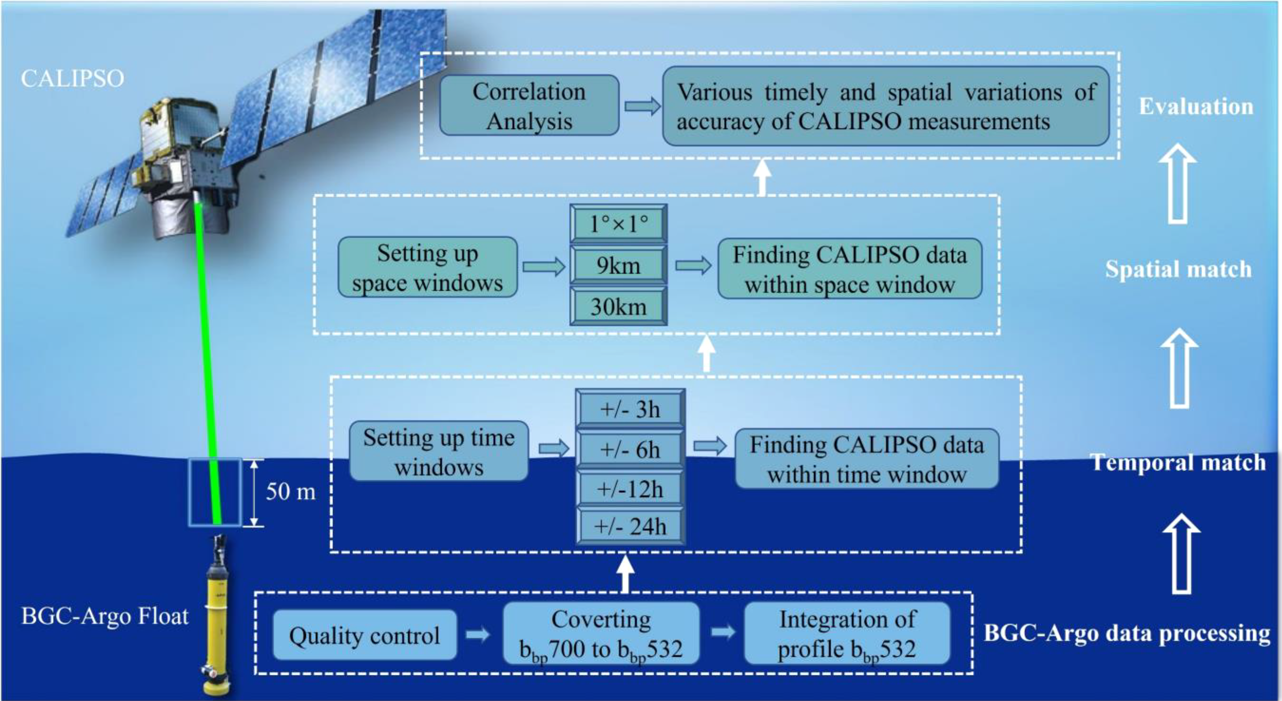
Presents the flow chart of this study.
where the power-law slope (γ) was set equal to 0.78 (Boss et al., 2013). Finally, for comparison with CALIOP and MODIS estimates, bbp(532) was depth-averaged with the following vertical weighting function (Haëntjens et al., 2017):
where Kd(532) is the diffuse attenuation coefficient of the downwelling irradiance at 532 nm (m−1). Kd(λ) was first computed at 490 nm by fitting a fourth-degree polynomial function on the logarithm of the downwelling irradiance Ed(490) measured by the floats (OCR-504, Satlantic Inc.) and then calculating the mean slope over the first 50 meters. Based on the quality-control procedure described in Organelli et al., only profiles of types 1 and 2 (for “good” and “probably good”, respectively) were used. In addition, each data point acquired along the profile flagged as “bad” or “probably bad” was removed. For 30% of the dataset, the quality of the profiles was too poor (type 3) to calculate Kd(490). In these cases, we used the average Kd(490) of profiles within a radius of 100 km and a time period of 20 days (the decorrelation scale of bio-optical properties), where bFLOATbp had changed by less than 50%. Kd(490) was then scaled to 532 nm according to (Lu et al., 2016):
Afterward, we conducted spatial and temporal match between in situ and satellite data. The high density of the float network allowed us to test three matchup configurations: (1) Single float profiles were colocated with the nearest 9 by 9 km MODIS pixel and CALIOP shots. At this spatial resolution, we set four time windows, which are +/- 3 h, +/- 6 h, +/- 12 h and +/- 24 h. (2) Float and CALIOP data were binned over 1° by 1° grid boxes and +/- 3 h, +/- 6 h, +/- 12 h and +/- 24 h periods. (3) Distances were extended to 30 km and four types of time windows. The spatial distribution of matching points and the number of matching points for each spatiotemporal window are depicted in Figure 3.
Figure 3
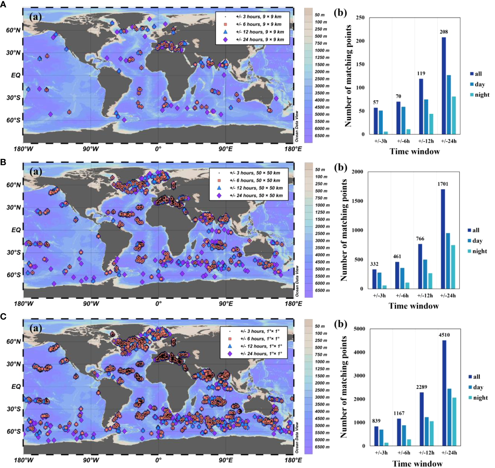
Shows the results for matching points using different spatial windows, including a 9 km window (A), a 50 km window (B), and a 1°×1° window (C). Additionally, the figure includes two subplots: (a) which displays the spatial distribution of matching points, and (b) which shows the number of matching points in each time window, including all, daytime, and nighttime. The black dots represent matching points with a time window of +/- 3 hours, orange squares represent matching points with a time window of +/- 6 hours, blue triangles represent matching points with a time window of +/- 12 hours, and purple diamonds represent matching points with a time window of +/- 24 hours.
2.4 Methodology for assessing CALIPSO bbp accuracy
We have selected the following five indicators to evaluate the quality of CALIPSO data. R-squared (R² or the coefficient of determination) is a statistical measure in a regression model that determines the proportion of variance in the dependent variable that can be explained by the independent variable (Nagelkerke, 1991). The formula is shown below:
where the numerator part represents the sum of the squared differences between the true and predicted values, and the denominator part represents the sum of the squared differences between the true and mean values.
The adjusted R-squared value is a modified version of R-squared that adjusts for predictors that are not significant in a regression model (Miles, 2005). The formula is shown below:
where n is the number of samples and p is the number of features.
The root mean square error (RMSE) is the square root of the ratio of the square of the deviation of the predicted value from the true value to the number of observations n (Chai and Draxler, 2014). It is used to measure the deviation of the observed value from the true value. The formula is shown below:
where Xi is the predicted value and Yi is the observed value.
The mean absolute percent error (MAPE) is the average of the distance between the model prediction and the sample true value (Coyle and Lin, 1988). The formula is shown below:
A MAPE of 0% indicates a perfect model, while a MAPE greater than 100% indicates a poor model.
The standard deviation (SD), mathematical symbol σ (sigma), is most often used in probability statistics as a measure of the degree of dispersion of a set of values (Beytas et al., 1983). The formula is shown below:
where μ is the average value.
3 Results
3.1 Various matchup configurations
We set three spatial windows (9 km (Figure 4), 30 km (Figure 5) and 1°×1° (Figure 6)) and four time windows (+/- 3 h, +/- 6 h, +/-12 h, +/-24 h) to obtain results for a total of 12 matching dimensions. Among these spatial and temporal windows, the best performance was obtained in the matching state with a spatial window of 9 km and a temporal window of +/- 3 h. The number of matching points obtained in this matching state was 58, the value of RMSE was 3.7×10⁻⁴ m-1, and the value of the relative coefficient was 0.80 (Figure 4A).
Figure 4
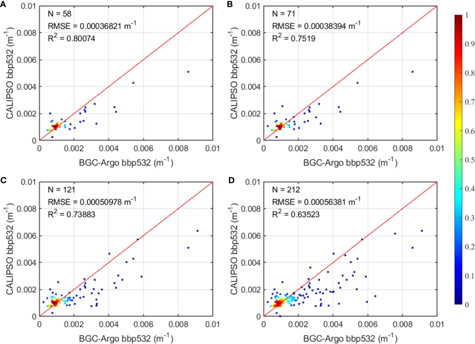
Displays the results of different temporal matching windows within a 9 km spatial window. The figure includes four subplots: (A) which shows the results for a +/- 3 hour time window, (B) which shows the results for a +/- 6 hour time window, (C) which displays the results for a +/- 12 hour time window, and (D) which shows the results for a +/- 24 hour time window.
Figure 5
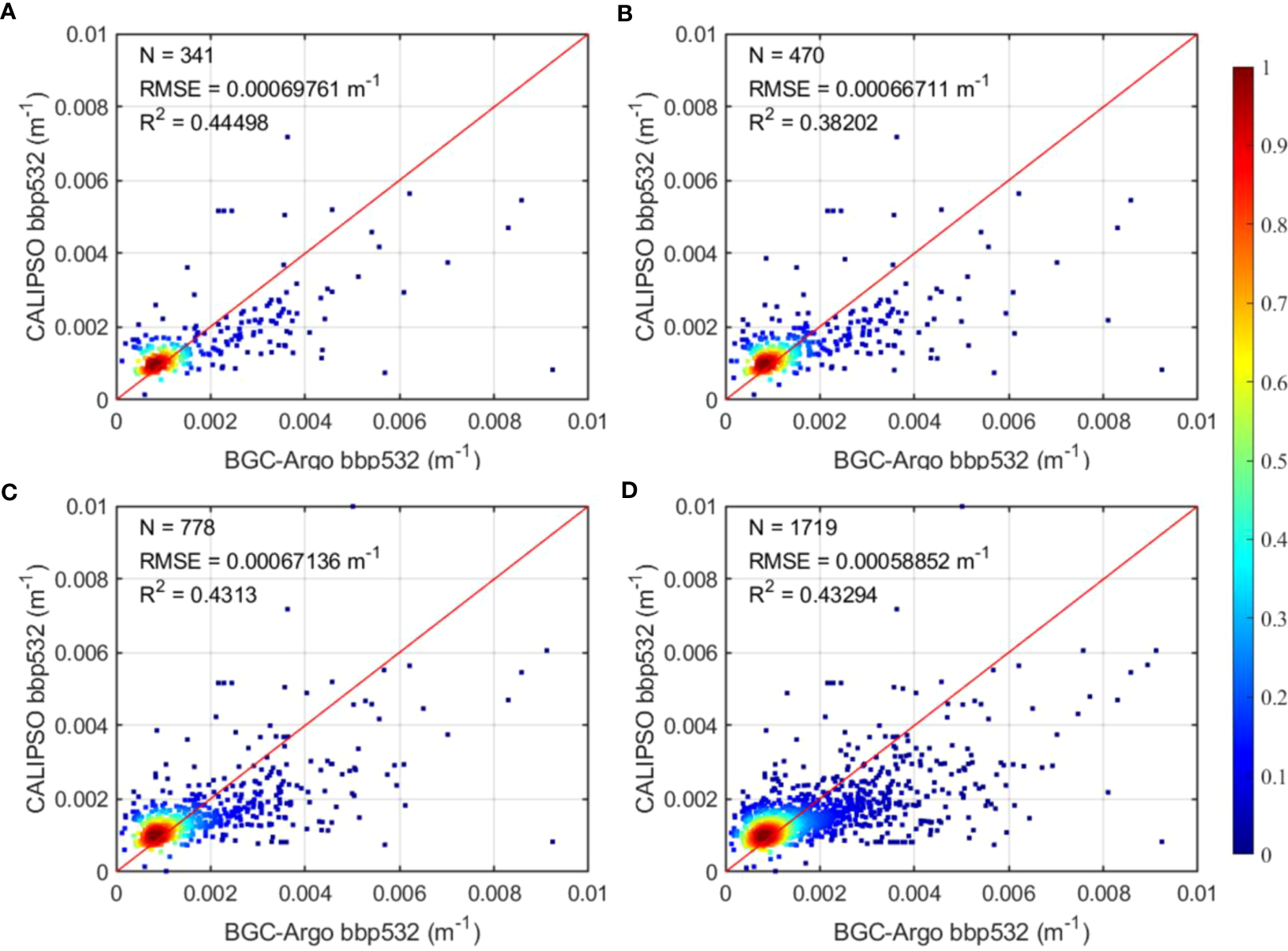
Shows the results of different temporal matching windows within a 50 km spatial window. The figure includes four subplots: (A) which displays the results for a +/- 3 hour time window, (B) which shows the results for a +/- 6 hour time window, (C) which displays the results for a +/- 12 hour time window, and (D) which shows the results for a +/- 24 hour time window.
Figure 6
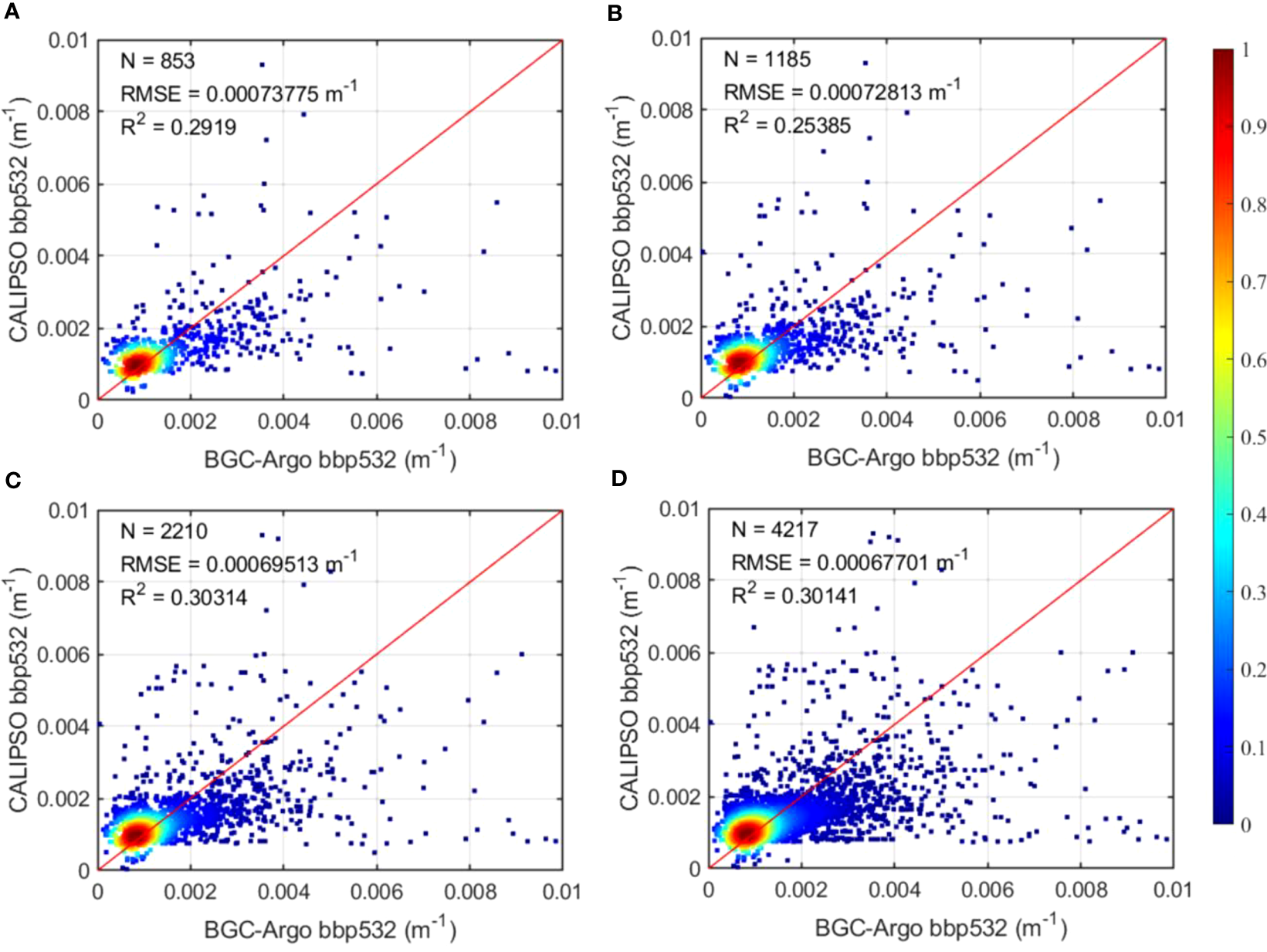
Displays the results of different temporal matching windows within a 1°×1° spatial window. The figure includes four subplots: (A) which shows the results for a +/- 3 hour time window, (B) which shows the results for a +/- 6 hour time window, (C) which displays the results for a +/- 12 hour time window, and (D) which shows the results for a +/- 24 hour time window.
For the matching points acquired under the +/- 3 h, +/- 6 h, +/- 12 h and +/- 24 h time windows, the data quality is best for 9 km in all three time windows. As the time span increases, a closer distance among the matching points indicates a more scientific and reliable assessment from the matching point of view. Within the same spatial window, the matching results for both the 9 km and 50 km spatial windows show a trend that the closer the time is, the more accurate the data are, but under the 1-degree spatial window, it reflects that the +/- 24 h time window is the best case for data accuracy (Figure 6D).
Therefore, to provide more accurate information for the evaluation and to ensure a sufficient number of matching points for discussing the data performance at spatial and temporal scales, we discussed and analyzed the matching results with a spatial window of 9 km and a temporal window of +/- 12 h in the following section (see Table 1 for a detailed evaluation of the data performance).
Table 1
| N | R-Squared | Adjusted R-square | RMSE/ m-1 | MAPE/% | SD | ||
|---|---|---|---|---|---|---|---|
| ALL (DAY+NIGHT) | |||||||
| Yearly | 2011 | 3 | 0.14 | – | 0.0003 | 9.1130 | 0.0002 |
| 2012 | 13 | 0.32 | 0.26 | 0.0004 | 27.8611 | 0.0004 | |
| 2013 | 16 | 0.80 | 0.78 | 0.0005 | 42.4683 | 0.0009 | |
| 2014 | 24 | 0.70 | 0.69 | 0.0007 | 34.9588 | 0.0009 | |
| 2015 | 30 | 0.84 | 0.84 | 0.0005 | 31.2262 | 0.0011 | |
| 2016 | 24 | 0.71 | 0.70 | 0.0005 | 32.9935 | 0.0006 | |
| 2017 | 11 | 0.72 | 0.69 | 0.0003 | 59.8987 | 0.0007 | |
| Seasonal | spring | 38 | 0.47 | 0.45 | 0.0004 | 51.3626 | 0.0007 |
| summer | 42 | 0.86 | 0.86 | 0.0006 | 24.0755 | 0.0009 | |
| autumn | 28 | 0.54 | 0.52 | 0.0004 | 30.3330 | 0.0010 | |
| winter | 14 | 0.15 | 0.08 | 0.0003 | 36.2397 | 0.0008 | |
| Spatial | Mediterranean Sea | 19 | 0.64 | 0.62 | 0.0004 | 93.7747 | 0.0004 |
| North Atlantic | 21 | 0.48 | 0.45 | 0.0014 | – | 0.0014 | |
| South Atlantic | 14 | 0.53 | 0.49 | 0.0010 | – | 0.0010 | |
| Indian Ocean | 34 | 0.64 | 0.63 | 0.0004 | – | 0.0004 | |
| North Pacific | 5 | 0.05 | – | 0.0010 | – | 0.0015 | |
| South Pacific | 8 | 0.51 | 0.43 | 0.0006 | – | 0.0006 | |
| DAY | |||||||
| Yearly | 2011 | 3 | 0.14 | – | 0.0003 | 9.1130 | 0.0002 |
| 2012 | 6 | 0.69 | 0.62 | 0.0001 | 17.3279 | 0.0001 | |
| 2013 | 9 | 0.91 | 0.90 | 0.0003 | 51.4637 | 0.0006 | |
| 2014 | 20 | 0.75 | 0.73 | 0.0006 | 33.1875 | 0.0007 | |
| 2015 | 17 | 0.93 | 0.92 | 0.0003 | 26.9816 | 0.0010 | |
| 2016 | 15 | 0.73 | 0.71 | 0.0005 | 25.1637 | 0.0005 | |
| 2017 | 7 | 0.74 | 0.69 | 0.0003 | 31.4123 | 0.0005 | |
| Seasonal | spring | 25 | 0.13 | 0.09 | 0.0004 | 43.0296 | 0.0006 |
| summer | 32 | 0.86 | 0.85 | 0.0005 | 19.6612 | 0.0007 | |
| autumn | 12 | 0.89 | 0.88 | 0.0002 | 24.8707 | 0.0006 | |
| winter | 8 | 0.10 | -0.05 | 0.0003 | 38.8639 | 0.0003 | |
| Spatial | Mediterranean Sea | 13 | 0.34 | 0.28 | 0.0004 | – | 0.0003 |
| North Atlantic | 14 | 0.68 | 0.65 | 0.0011 | – | 0.0011 | |
| South Atlantic | 9 | 0.87 | 0.85 | 0.0004 | – | 0.0003 | |
| Indian Ocean | 22 | 0.68 | 0.66 | 0.0005 | – | 0.0005 | |
| North Pacific | – | – | – | – | – | – | |
| South Pacific | 6 | 0.41 | 0.26 | 0.0007 | 83.8254 | 0.0007 | |
| NIGHT | |||||||
| Yearly | 2011 | – | – | – | – | – | – |
| 2012 | 7 | 0.34 | 0.21 | 0.0005 | 36.8896 | 0.0005 | |
| 2013 | 8 | 0.75 | 0.71 | 0.0005 | 31.3615 | 0.0011 | |
| 2014 | 4 | 0.70 | 0.54 | 0.0011 | 43.8155 | 0.0011 | |
| 2015 | 13 | 0.80 | 0.78 | 0.0007 | 36.7768 | 0.0013 | |
| 2016 | 9 | 0.81 | 0.78 | 0.0003 | 46.0432 | 0.0007 | |
| 2017 | 4 | 0.93 | 0.90 | 0.0002 | – | 0.0011 | |
| Seasonal | spring | 13 | 0.68 | 0.65 | 0.0005 | 67.3876 | 0.0008 |
| summer | 10 | 0.91 | 0.90 | 0.0006 | 39.2508 | 0.0012 | |
| autumn | 16 | 0.44 | 0.40 | 0.0006 | 34.4298 | 0.0012 | |
| winter | 6 | 0.31 | 0.14 | 0.0004 | 32.7408 | 0.0010 | |
| Spatial | Mediterranean Sea | 7 | 0.85 | 0.82 | 0.0004 | 66.4020 | 0.0003 |
| North Atlantic | 7 | 0.37 | 0.25 | 0.0017 | – | 0.0017 | |
| South Atlantic | 5 | 0.14 | – | 0.0017 | – | 0.0018 | |
| Indian Ocean | 12 | 0.35 | 0.28 | 0.0002 | – | 0.0003 | |
| North Pacific | 4 | 0.00 | – | 0.0007 | – | 0.0013 | |
| South Pacific | – | – | – | – | – | – | |
Performance metrics of daytime and nighttime bbp in detail from interannual, seasonal and temperature zones in a spatial window of 9 km and a time window of +/- 12 h.
3.2 Annual variation in the accuracy of CALIPSO measurements
We obtained a total of 121 matching points with a time window of +/- 12 h and a spatial window of 9 km, among which the number of matching points in 2015 was the largest, and the number of matching points in daytime and nighttime was close to each other, with slightly more matching points in daytime (Figure 7A).
Figure 7
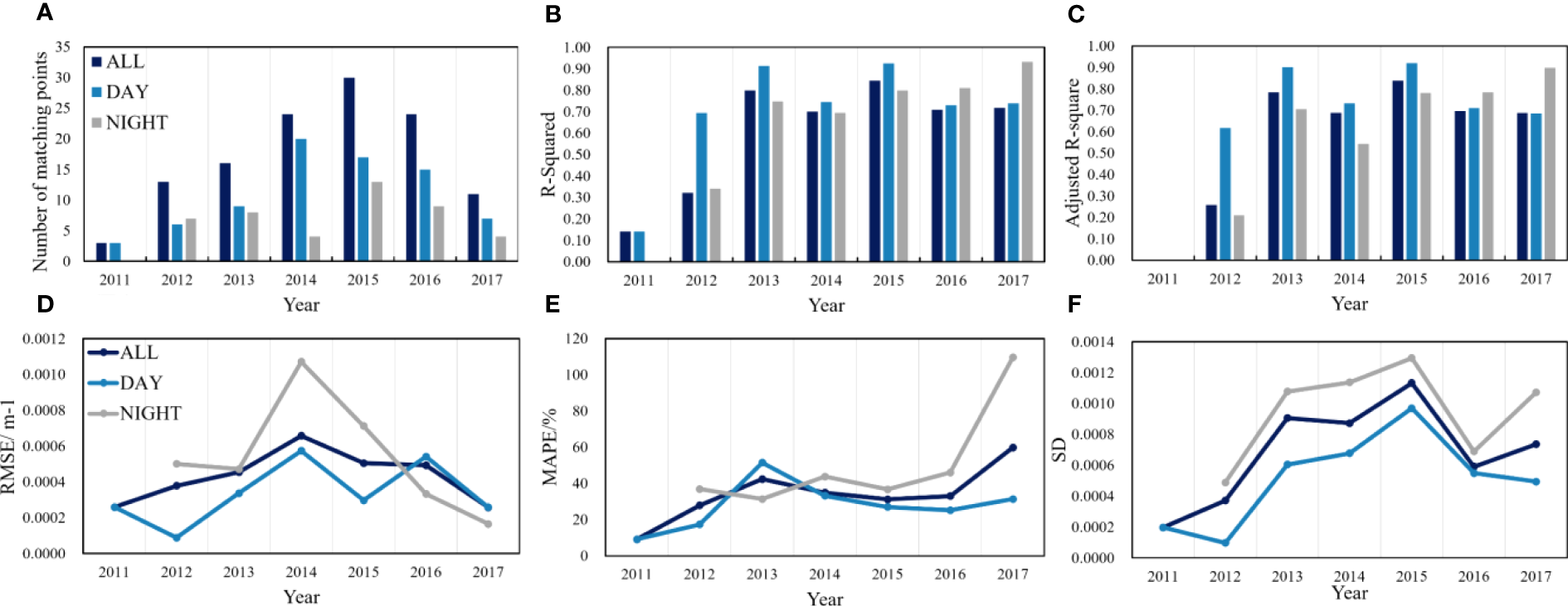
Shows the changes in annual accuracy of CALIPSO observations, based on the results of the matching point data fit evaluation within a 9 km spatial window and a +/- 12 hour time window. (A) represents the interannual variability of the number of matching points. (B) denotes the interannual variability of R-squared between CALIPSO products and BGC-Argo. (C) signifies the interannual variability of adjusted R-squared between CALIPSO products and BGC-Argo. (D) represents the interannual variability of RMSE of CALIPSO products. (E) indicates MAPE of CALIPSO products. (F) represents the interannual variability of SD of CALIPSO products.
In terms of interannual variation, the correlation of determination between bbp measured by CALIPSO and bbp observed by BGC-Argo were higher than 0.7 from 2013 to 2017, with a high of 0.84 in 2015 (Figure 7B). Using BGC-Argo detected bbp data to verify the accuracy of bbp data acquired by CALIPSO during daytime and nighttime, we found that the highest R2was during daytime in 2015 and during nighttime in 2017 (Table 1). From 2012 to 2017, the correlation coefficients were higher during the day than during the whole day and were higher than 0.9 in 2013 and 2015. The nighttime data, however, show a significantly higher data accuracy for 2015-2017 than for 2011-2014. Comparing the difference between daytime and nighttime data accuracy by year, we found that the difference between daytime and nighttime correlation coefficients was within 0.1 in 2014 and 2016 and up to 0.3 or more in 2012. The adjusted correlation coefficient is consistent with the trend exhibited by the uncorrected one (Figure 7C).
The RMSE was within 0.0011 m-1 for each year from 2011-2017 (Table 1), with the maximum value occurring in 2014 for both daytime and nighttime, but the year in which the minimum value was located differed, with the minimum value of the RMSE in 2012 for daytime and in 2017 for nighttime (Figure 7D). The average absolute percentage error for each year from 2011-2017 was within 59.9%, with the largest in 2017 and the smallest in 2011 (Figure 7E). The standard deviation of the CALIPSO bbp values was within 0.0011 for each year from 2011-2017, with the largest standard deviation of the CALIPSO bbp values occurring in 2015 and the smallest standard deviation in 2011 (Figure 7F).
3.3 Seasonal variation in the accuracy of CALIPSO measurements
Since the CALIPSO data to be evaluated cover the whole world, when we performed the seasonal analysis, we divided the seasons for each of the Northern and Southern Hemispheres, so the seasonal distribution of the obtained evaluation results was applied to the local seasons. At the level of the number of matching points acquired, the highest number was obtained in spring and the lowest was obtained in winter, with the difference between the two numbers nearly doubling.
We found the most accurate data for summer with a correlation coefficient of 0.86, but the summer product also had the highest RMSE (Figure 8). The elevated RMSE of the product during the summer season can likely be attributed to the transport of land-sourced dust over the ocean. This phenomenon aligns with the findings of Xiaomin et al. (2023), who reported an annual cycle of aerosol optical depth at 550 nm (AOD550) with a peak in July, primarily driven by dust transport(Xiaomin et al., 2023). In terms of the correlation coefficient, except for autumn, all seasons show a trend of more accurate nighttime data than daytime data. The reason for the superior quality of daytime data compared to nighttime data in autumn could be linked to the South Atlantic Anomaly (SAA). The SAA has a notable impact on the backscatter coefficient observations made by CALIPSO during nighttime, causing an elevation in random fluctuations within the recorded signal. This effect is further compounded by increased particle flux, resulting in a significantly higher dark noise level in the 532 nm channel during SAA, which is reported to be 30 times greater. Consequently, the signal-to-noise ratio (SNR) experiences a fivefold decrease at night (Hunt et al., 2009). The largest difference was found in spring, with a correlation coefficient between bbp measured by CALIPSO and bbp observed by BGC-Argo of 0.13 for spring bbp during the day but a correlation coefficient of 0.68 at night (Table 1). The daytime correlation coefficients are high in summer and autumn and low in spring and winter, but the nighttime correlation coefficients are high in spring and summer and low in autumn and winter. The nighttime correlation coefficient in summer was as high as 0.91 (Table 1), making it the season with the closest data to the BGC-Argo float observed data of all seasons. MAPE is the smallest for summer products and the largest for spring (Figure 8). The standard deviation of the products varied little from season to season, with the maximum occurring in autumn.
Figure 8
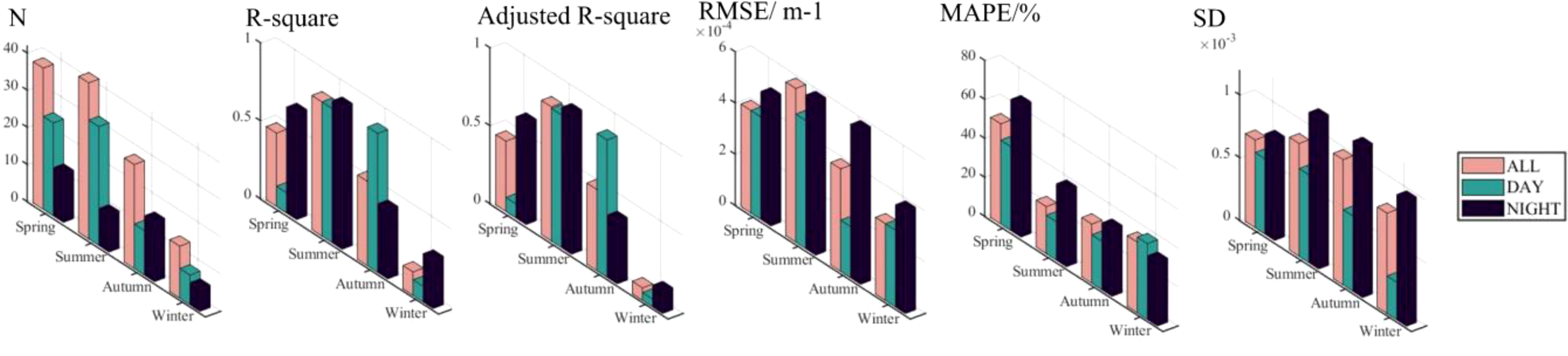
Displays the changes in annual season of CALIPSO measurements, based on the results of the matching point data fit evaluation within a 9 km spatial window and a +/- 12 hour time window.
3.4 Spatial variation in the accuracy of CALIPSO measurements
Since the number of matched sites located in the Arctic and Southern Oceans is too small, we selected six sea areas in other global seas (Region 1 for the Mediterranean Sea, Region 2 for the North Atlantic, Region 3 for the South Atlantic, Region 4 for the Indian Ocean, Region 5 for the North Pacific, and Region 6 for the South Pacific) as typical regions for spatial comparison of data quality. As seen from the bar chart in Figure 9, the Mediterranean Sea region has the best data quality performance among the six sea areas, with the highest R-squared and the lowest RMSE, MAPE and SD (Table 1, R-Squaredregion 1 = 0.64, RMSEregion 1 = 3.9×10⁻⁴ m-1, MAPE region 1 = 93.77%, SDregion 1 = 3.8×10⁻⁴). The Indian Ocean data quality is second only to the Mediterranean and better than the Atlantic and Pacific (Table 1, R-Squaredregion 4 = 0.64, RMSEregion 4 = 4.2×10⁻⁴ m-1, MAPEregion 4 = 140.72%, SD region 4 = 4.2×10⁻⁴). We postulate the observed decrease in product performance specifically in the Indian Ocean region, which is associated with Aerosol Optical Depth (AOD). Previous research has indicated that marine aerosols in this region are predominantly influenced by land-based sources, such as dust and biomass burning (Li et al., 2014; Ma et al., 2021; Xiaomin et al., 2023). These aerosols are transported from the West African coast to the North Arabian Sea through distinct dust patterns. The higher concentration of Aerosol Optical Depth in the Indian Ocean region introduces significant noise into the CALIPSO data, leading to a noticeable decline in product performance. Using the equator as the dividing line and comparing the data quality situation in the North and South Atlantic, the data quality in the South Atlantic is somewhat better (Table 1, R-Squaredregion 2 = 0.48, R-Squaredregion 3 = 0.53, RMSEregion 2 = 1.4×10⁻³ m-1, RMSEregion 3 = 1.0×10⁻³ m-1). Similarly, using the equator as the dividing line, a comparison of the North and South Pacific reveals that the Pacific Ocean exhibits better data quality south of the equator (Table 1, R-Squaredregion 5 = 0.05, R-Squaredregion 6 = 0.51, RMSEregion 5 = 1.0×10⁻³ m-1, RMSEregion 6 = 6.0×10⁻⁴ m-1), as does the Atlantic Ocean. According to recent studies by Xiaomin et al. (2023), the annual mean Aerosol Optical Depth at a wavelength of 550 nanometers (AOD550) in the northern hemisphere (0.187–0.207) is significantly greater compared to the southern hemisphere (0.110–0.135) (Xiaomin et al., 2023). Based on this observation, we speculate that the elevated AOD levels in the northern hemisphere, including the Pacific and Atlantic regions, have an impact on LIDAR detection, resulting in higher noise levels in the CALIPSO product as compared to the southern hemisphere. We used 0.3 as the threshold to distinguish high Aerosol Optical Depth (AOD) cases (spatial distribution can be seen in Figure 10A). We removed the matching points between CALIPSO and BGC-Argo under the high AOD conditions within a 9 km, +/- 12 h spatiotemporal window. We found that the high AOD values were predominantly located in the Northern Hemisphere. After removing these high AOD values, the number of matching points decreased to 116 (Figure 10B). Furthermore, the R2 between CALIPSO bbp and BGC-Argo bbp improved after the removal of high AOD values compared to the situation where no removal was performed (R2before = 0.739, R2after = 0.742, Figure 10C). Additionally, the Mean Absolute Percentage Error (MAPE) decreased after the removal of high AOD values compared to the situation where no removal was performed (MAPEbefore = 35.50%, MAPEafter = 32.84%, Figure 10D).
Figure 9
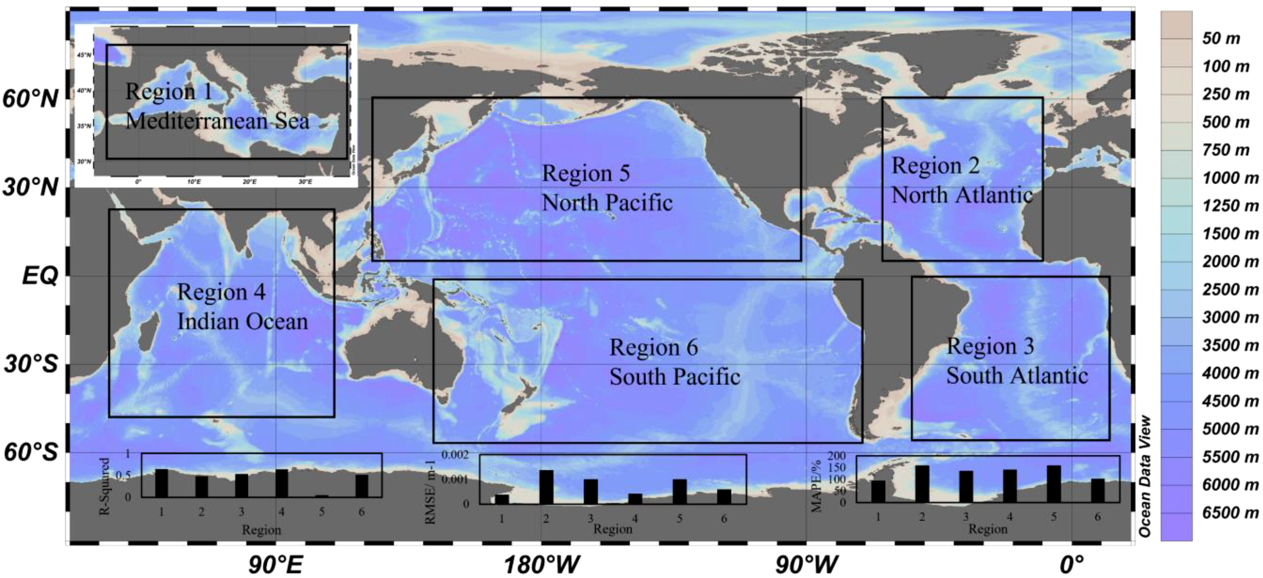
Shows the classification of study sea areas and the results of data evaluation for each sea area, based on the matching point data fit evaluation within a 9 km spatial window and a +/- 12 hour time window.
Figure 10
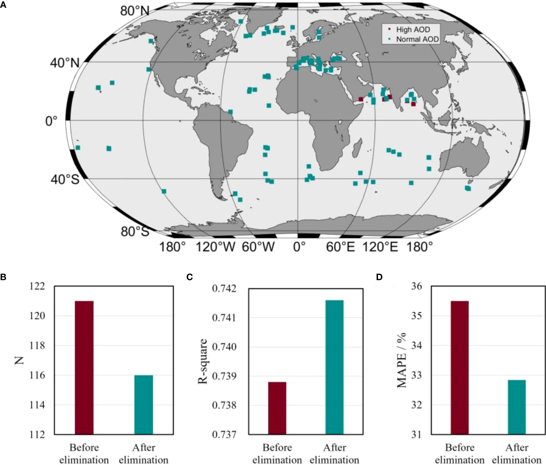
Illustrates the comparison of matching points between CALIPSO and BGC-Argo before and after removing high Aerosol Optical Depth (AOD) values within a 9 km, +/- 12 h window. (A) shows the spatial distribution comparison of matching points between CALIPSO and BGC-Argo corresponding to high AOD values and normal AOD values within the 9 km, +/- 12 h window. (B) presents the comparison of the number of matching points between CALIPSO and BGC-Argo before and after removing high AOD values. (C) displays the correlation coefficient between CALIPSO bbp and BGC-Argo bbp before and after removing high AOD values. (D) represents the Mean Absolute Percentage Error (MAPE) between CALIPSO bbp and BGC-Argo bbp before and after removing high AOD values.
Furthermore, CALIOP lidar measurements can be affected by the presence of severe wind conditions. Elevated wind speeds can lead to signal contamination due to the presence of bubbles, foam, and whitecaps on the ocean’s surface. Conversely, during periods of low-wind conditions, intense specular reflection originating from the sea surface may cause saturation errors within the co-polarized channels. These observations have been documented in previous studies (Behrenfeld et al., 2013; Lu et al., 2014b) and contribute to regional disparities in the precision of CALIPSO measurements. We used 6 m/s as the threshold to distinguish high wind speed conditions (spatial distribution can be seen in Figure 11A). We removed the matching points between CALIPSO and BGC-Argo within a 9 km, +/- 12 h spatiotemporal window when the wind speed exceeded 6 m/s. After removing these high wind speed values, the number of matching points decreased to 101 (Figure 11B). Furthermore, the R2 between CALIPSO bbp and BGC-Argo bbp improved after the removal of high wind speed values compared to the situation where no removal was performed (R2before = 0.739, R2after = 0.742, Figure 11C). Additionally, the Mean Absolute Percentage Error (MAPE) decreased after the removal of high wind speed values compared to the situation where no removal was performed (MAPEbefore = 35.50%, MAPEafter = 34.00%, Figure 11D).
Figure 11

Illustrates the comparison of matching points between CALIPSO and BGC-Argo before and after removing high wind speed values within a 9 km, +/- 12 h window. (A) shows the spatial distribution comparison of matching points between CALIPSO and BGC-Argo corresponding to high wind speed values and normal wind speed values within the 9 km, +/- 12-hour window. (B) presents the comparison of the number of matching points between CALIPSO and BGC-Argo before and after removing high wind speed values. (C) displays the correlation coefficient between CALIPSO bbp and BGC-Argo bbp before and after removing high wind speed values. (D) represents the Mean Absolute Percentage Error (MAPE) between CALIPSO bbp and BGC-Argo bbp before and after removing high wind speed values.
In addition to wind conditions, the inherent optical properties of seawater are influenced by temperature and salinity ancillary values (Sullivan et al., 2006; Zhang et al., 2009). The backscattering by pure seawater (bbw) can exhibit variations of up to 25% along salinity (primarily) and temperature gradients (Sullivan et al., 2006; Zhang et al., 2009; Werdell et al., 2013). The current CALIPSO bbp inversion model lacks explicit consideration of the effects of temperature and salinity, which may impact the accuracy of CALIPSO bbp products. These regional differences in temperature and salinity, which affect the scattering of seawater, can interfere with the inversion of the bbp product, consequently leading to regional variations in the performance of the product. In order to enhance the performance of these products, we suggest incorporating the effects of temperature and salinity in future CALIPSO bbp inversions. By doing so, we anticipate significant improvements in the accuracy and reliability of the CALIPSO bbp products.
Moreover, apart from the oceanic factors, it is important to consider the impact of algorithms on product accuracy. The χ factor associated with particles (χp) is significantly influenced by the shape and internal structure of particles (Meyer, 1979; Bohren and Singham, 1991; Ulloa et al., 1994; Zhang et al., 2021). Additionally, it varies among different phytoplankton species and shows substantial variations across diverse seas (Boss and Pegau, 2001a; Chami et al., 2006; Berthon et al., 2007; Zhang et al., 2014; Harmel et al., 2016). Consequently, applying a constant χp value to interpret lidar signals obtained from various water bodies introduces significant errors, as supported by the observed differences in product performance over the sea.The study by V. Noel et al. found that above the South Atlantic Anomaly (SAA), CALIOP dark noise levels fluctuated by ±6% between 2006 and 2013 and followed a known inverse correlation (with a 1-year lag) between local particle fluxes and the 11-year cycle of solar activity. With the start of the 24th cycle of solar activity, the noise in the SAA region decreases accordingly, and V. Noel et al. expect that the noise may reach a minimum in 2014 (Noel et al., 2014). Therefore, we explore the quality of CALIPSO nighttime bbp products for the SAA region. Due to the limited number of matches, we chose the largest spatiotemporal window (1° × 1°, 24 h) to ensure that CALIPSO and BGC-Argo have enough matching points in each year for discussion. It was found that in 2014 CALIPSO’s bbp product reached the lowest MAPE between 2012-2017, at 16.88% (Figure 12). This is in agreement with the predicted results of the study by V. Noel et al.
Figure 12
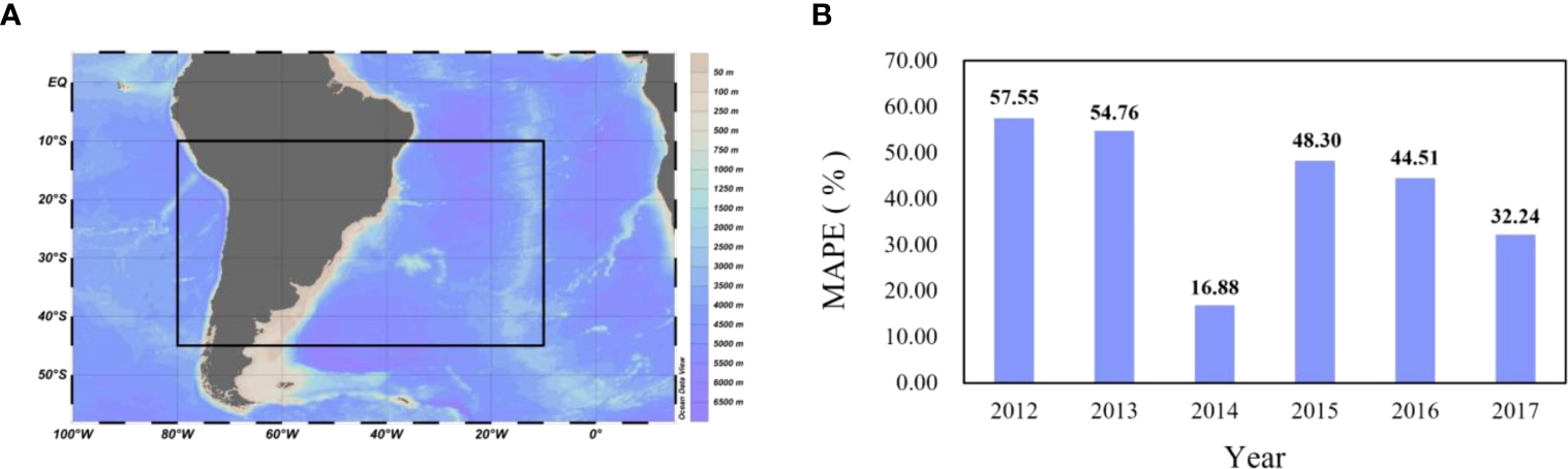
Illustrates the interannual variation of MAPE for the nighttime bbp product of CALIPSO in the South Atlantic Anomaly (SAA) (the region ranges from 80°W-10°W and 10°S-45°S). (A) represents the spatial extent of the SAA region, while (B) indicates the interannual variability of the Mean Absolute Percentage Error (MAPE) of the CALIPSO nighttime bbp product in this region based on BGC-Argo.
4 Discussion
4.1 Comparisons of bbp estimates between CALIPSO and MODIS
A regional evaluation analysis was performed by Lacour et al. in 2020 using different spatial windows (9 km, 1 and 2 degree grids) and a 16-day time window (Lacour et al., 2020), which found a relative error of 13% for CALIOP observations compared to Argo buoy data, and this value is greater than that of MODIS-Aqua bbp data. However, the performance analysis of Lacour et al. used Argo Kd data to calculate CALIOP bbp without correcting for detector interference, and there were sampling biases between CALIOP and MODIS-Aqua, so the regional average of CALIOP was not necessarily the same as the average of MODIS-Aqua. In the study by Lu et al. (Lu et al., 2021), CALIOP and Argo buoy data were compared globally on coarse spatial and temporal scales (1 degree per month spatial-temporal window with 1-300 observations per window). They found that the agreement between CALIOP and Argo bbp improved after correcting for crosstalk, with the relative difference decreasing from 36% to 5%, but their root mean square difference did not change (~10-3 m-1). Bisson et al. in 2021 (Bisson et al., 2021) compared the BGC-Argo data with Behrenfeld et al. in their 2019 study (Behrenfeld et al., 2019) using a global comparison of CALIOP data, starting with a decorrelation scale analysis to identify appropriate temporal and spatial windows for overlap, and they quantified the spatial and temporal scales at which Spearman’s correlation slope decreases significantly, using spatial scales of up to 50 km and temporal matches of +/-3 h and +/-24 h. The comparison shows that the CALIOP retrieval outperforms MODIS-Aqua, with a relative error of less than 20% for CALIOP compared to 25% for MODIS-Aqua.
Evaluating the equivalent matching data between Argo observations of bbp and CALIOP retrievals and MODIS retrievals using matching results for a 9 km spatial window and 12 h time window, we found that CALIOP has superior performance (Figures 13B, D) with higher R2 (R2CALIPSO=0.7388, R2MODIS=0.5072) and lower RMSE (RMSECALIPSO=5.0×10⁻⁴ m-1, RMSEMODIS=7.0×10⁻⁴ m-1). At the same location of CALIPSO and MODIS, CALIPSO still shows better performance (Figures 13B, F) with higher R2 (R2CALIPSO=0.7388, R2MODIS=0.4385) and lower RMSE (RMSECALIPSO=5.0×10⁻⁴ m-1, RMSEMODIS=8.0×10⁻⁴ m-1). Moreover, the bbp obtained by CALIPSO observation is closer to that observed by BGC-Argo in terms of the slope of the fitted line, and the bbp obtained by MODIS observation is slightly larger than that obtained by BGC-Argo observation (Figures 13A, C, E). However, after limiting MODIS and CALISPO at the same position, the bbp obtained from the MODIS observation has no significant slope deviation from the bbp observed by BGC-Argo. Upon comparing Figures 13D, F, it becomes evident that the MODIS-detected bbp values are consistently higher than the BGC-Argo measured values, primarily in the region characterized by lower values around 10-3. The percent error interval of bbp detected by CALIPSO was smaller and showed superior performance (Figures 14A, B), especially for larger values of bbp. CALIPSO showed better consistency compared to MODIS. Within the consistency range, the absolute value of the difference between bbp measured by BGC-Argo and bbp measured by CALIPSO is up to 0.0019 m-1, and the average value of the difference is 0.0002 m-1. The absolute value of the difference between bbp measured by BGC-Argo and bbp measured by MODIS is up to 0.0020 m-1, and the average value of the difference is also 0.0002 m-1.
Figure 13
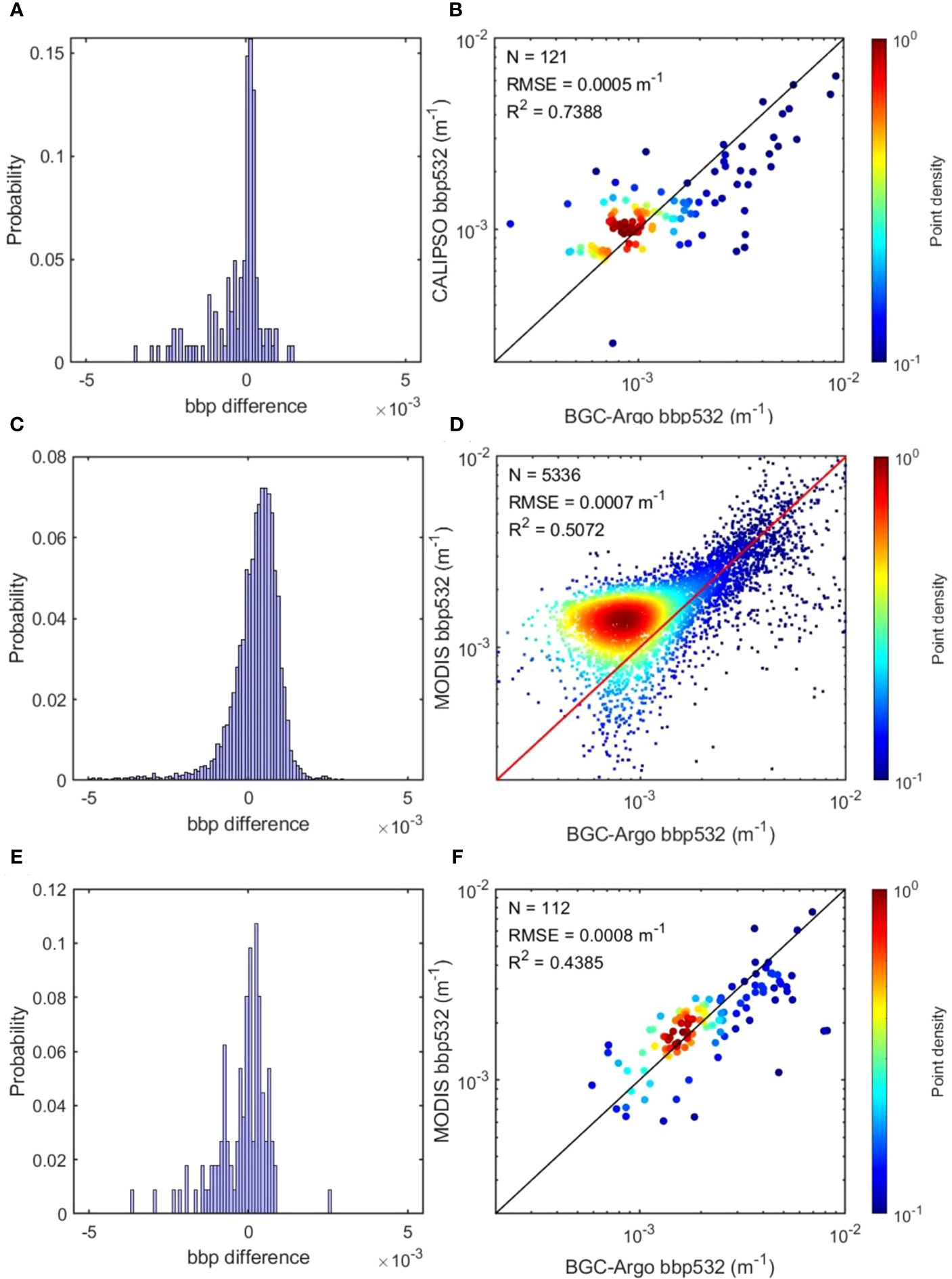
Displays the comparison between CALIPSO and BGC-Argo bbp (532 nm) matchups for a 9 km spatial window and a +/- 12 hour time window, as well as the comparison between MODIS and BGC-Argo bbp (532 nm) matchups for the same spatial and temporal window. (A, B) denote the fitting results of CALIPSO and BGC-Argo matching, (C, D) denote the fitting results of MODIS and BGC-Argo matching (all matching points), and (E, F) denote the fitting results of MODIS and BGC-Argo matching (matching points of MODIS and CALIPSO at the same position).
Figure 14
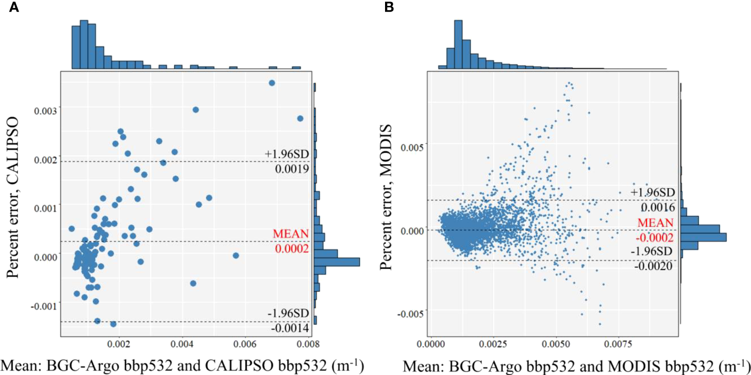
Includes two subplots: (A) displays a Bland-Altman plot between CALIPSO and BGC-Argo, with the x-axis representing the mean of paired (CALIPSO, Argo) observations and the y-axis representing the percent error of CALIPSO, and (B) shows a Bland-Altman plot between MODIS and BGC-Argo, with the x-axis representing the mean of paired (MODIS, BGC-Argo) observations and the y-axis representing the percent error of MODIS. The probability distributions for MODIS, CALIOP, and BGC-Argo bbp (532 nm) are included on the top of each plot.
4.2 Comparisons of bbp estimates between daytime and nighttime
Due to the effect of solar background radiation, the performance of lidar is much worse during daytime operation than during nighttime operation, and the signal-to-noise ratio is lower during daytime than during nighttime (Behrenfeld et al., 2013). However, the evaluation results of all seasons under the 9 km spatial window and +/- 12 h time window in the previous paper show that the RMSE of the daytime product is smaller (Figure 8). To evaluate the product performance more accurately, we narrowed the time window and selected a 9 km, +/- 3 h spatiotemporal window, so the definition of the daytime and nighttime periods is more strictly controlled (Figure 15A). Due to the small number of matching points under the hourly spatial window, the results show that the performance of CALIPSO nighttime products is slightly better than that of daytime products in spring (Figure 15C, RMSECALIPSO=3.0×10⁻⁴ m-1, RMSENIGHT=2.0×10⁻⁴ m-1). However, all other evaluated parameters show a slightly better quality of the daytime product than the nighttime product (Figures 15B, D, E). There is a polarization gain ratio error in CALIPSO’s nighttime results; the nighttime backscattering depolarization ratios of land surfaces are very different from the daytime measurements, and the nighttime depolarization ratios are approximately 7% lower than the daytime measurements (Hu et al., 2021). We speculate that this is related to the sea surface wind speed; when the sea surface wind speed is higher at night, the intensity generated by the sea surface has a very strong impact on lidar observation. On the other hand, telluride radiation in SAA induces free current spikes and a large amount of dark noise in CALIOP nighttime measurements, which also has an impact on nighttime measurements (Hunt et al., 2009; Noel et al., 2014).
Figure 15

Compares the performance of daytime and nighttime CALIPSO products. The figure includes five subplots: (A) compares the correlation coefficients between daytime and nighttime products under two temporal windows (9 km, +/- 3 h and +/- 12 h), (B) shows the corrected correlation coefficients between daytime and nighttime products under the same temporal windows, (C) compares the root mean square error between daytime and nighttime products under the same temporal windows, (D) compares the mean absolute percent error between daytime and nighttime products under the same temporal windows, and (E) compares the standard deviation between daytime and nighttime products under the same temporal windows.
4.3 Correction of the β(π)/bbp conversion factor based on BGC-Argo
In previous studies, varying the β(π)/bbp conversion factor greatly affected the data quality, and Bission et al. doubled β(π)/bbp to produce different evaluation results from Lacour (Lacour et al., 2020; Bisson et al., 2021). In a study by Zhang et al., it was discovered that the conversion factor χp for particles, which is crucial for converting volume scattering functions (VSFs) to bbp at different scattering angles, exhibits a varying rate of change as the angle deviates from 120° (Zhang et al., 2021). However, the current CALIOP data processing assumes a fixed value of α (anisotropy factor), the ratio of the 180° backscatter to the average volume scattering function value between 90-180°, as 1 (Behrenfeld et al., 2022), overlooking the variability in the VSF-to-bbp conversion for different angles. To address this discrepancy, we propose investigating the conversion factor of β(π)/bbp at various spatial and temporal scales, providing a means to account for the associated error. Therefore, it is important to discuss the impact of the β(π)/bbp conversion factor on the CALIPSO performance at different times and locations and to quantify the optimal β(π)/bbp values for different locations and time scales.
Firstly, we obtained β(π) of CALIPSO corresponding to CALIPSO by substituting 0.32 of β(π)/bbp into the formula, and then replaced bbpCALIPSO(532) using bbpBGC-Argo(532) as the standard value to obtain the corrected conversion factor β(π)/bbp for each matching point. Then We calibrated the β(π)/bbp conversion factors for different years, seasons, and seas based on BGC-Argo buoy data. The conversion factors for 2011-2017 were above 0.2 (Figure 16A), the conversion factor for 2017 was the largest (β(π)/bbp =0.4117), and the conversion factor for 2011 was the smallest (β(π)/bbp = 0.2922). The conversion factors were above 0.3 for different seasons (Figure 16B), and the conversion factor was the largest in spring (β(π)/bbp =0.4099) and the smallest in summer (β(π)/bbp =0.3002). The conversion factors of different seas also differ (Figure 16C), with the conversion factor of 0.3100 in the Mediterranean Sea and 0.3820 in the Indian Ocean. The conversion factors of both the Atlantic and Pacific Oceans are larger in the north than in the south, with conversion factors of 0.3959 in the North Atlantic, 0.3617 in the South Atlantic, 0.3835 in the North Pacific, and 0.3835 in the South Pacific. The conversion factor was 0.3835 for the North Atlantic, 0.3617 for the South Atlantic, 0.2922 for the North Pacific, and 0.2922 for the South Pacific (Table 2). The seasonal differences in theβ(π)/bbp values may be caused by seasonal differences in phytoplankton morphology. Silvia Pulina et al. found that phytoplankton cells had a higher mean volume and lower mean surface area ratio in winter (in the deepest mixed layer) and various geometries in spring (at the lowest nutrient concentrations), with simple and compact geometries (spheres and cubes) having a lower mean volume and higher mean surface area ratio with simple and elongated geometries (cylinders) in summer (under thermally stratified conditions) and a variety of geometries in autumn (under moderate environmental conditions) (Pulina et al., 2022).
Figure 16
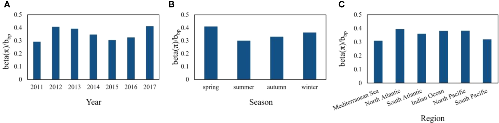
Shows the best values of β(π)/bbp from 2011-2017 (A), for each season (B), and for different regions (C).
Table 2
| Year | 2011 | 2012 | 2013 | 2014 | 2015 | 2016 | 2017 |
|---|---|---|---|---|---|---|---|
| β(π)/bbp | 0.2922 | 0.4075 | 0.3922 | 0.3469 | 0.3045 | 0.3247 | 0.4117 |
| Confidence Interval | [0.25,0.32] | [0.37,0.51] | [0.32,0.46] | [0.29,0.47] | [0.25,0.34] | [0.27,0.42] | [0.29,0.82] |
| Season | spring | summer | autumn | winter | |||
| β(π)/bbp | 0.4099 | 0.3002 | 0.3305 | 0.3636 | |||
| Confidence Interval | e | [0.27,0.33] | [0.29,0.38] | [0.29,0.45] | |||
| Region | Mediterranean Sea | North Atlantic | South Atlantic | Indian Ocean | North Pacific | South Pacific | |
| β(π)/bbp | 0.3100 | 0.3959 | 0.3617 | 0.3821 | 0.3835 | 0.2922 | |
| Confidence Interval | [0.28,0.34] | [0.31,0.52] | [0.29,0.46] | [0.34,0.51] | [0.21,0.60] | [0.25,0.38] | |
Best β(π)/bbp values in detail from interannual, seasonal and spatial scales in a spatial window of 9 km and a time window of +/- 12 h.
4.4 Quality control of BGC-Argo floats
Since the BGC-Argo buoy uses a disposable delivery method, it is difficult to perform frequent calibration of the sensors it carries, and it is also difficult to determine the cause of sensor errors after drifting in the ocean (Wong et al., 2020; Takatsuki et al., 2002). Therefore, quality control of the BGC-Argo buoy is necessary to ensure the quality of its actual measurement data.
There are two modes of quality control for BGC-Argo profiling buoy data: real-time quality control mode and time-delayed quality control mode. Real-time quality control means quality control within 24-72 hours after data generation, which is characterized by fast and short processing times and average data accuracy, but there are no obvious errors. Time-delayed quality control indicates quality control within 90 days after data generation, and the data quality can be reliably guaranteed by the information processed in this mode, which is suitable for scientific research (Schmechtig and Thierry, 2015).
Version 1.0 of the Argo Biogeochemical Data Quality Control Manual lists two quality control tests for bbp, including spike testing and global range testing, but the current BGC-Argo program has not formally released any documentation of quality control procedures for bbp parameters. Recently, Giorgio Dall’Olmo et al. proposed a new and more comprehensive real-time quality control model for bbp, which includes a missing data test, high depth value test, negative value test, noise profile test, and parking hook test (Dall'Olmo et al., 2022). Therefore, when the BGC-Argo quality control model matures, its reliability as real-world information for assessment will be further improved. The BGC-Argo quality control for CALIPSO bbp assessment will be further investigated.
5 Conclusions
The continued use of a large number of BGC-Argo buoys has given us the opportunity to evaluate the performance of CALIPSO bbp products at a finer spatial-temporal scale. We evaluated the performance of CALIPSO-retrieved bbp products using the bbp data detected by BGC-Argo buoys at 12 spatial and temporal windows and found that the CALIPSO products exhibited higher quality at more precise matching scales. We discuss the performance differences in the products at different interannual, seasonal, and spatial times using the matching results with a spatial window of 9 km and a temporal window of +/- 12 h. For the matching points acquired under the +/- 3 h, +/- 6 h, +/- 12 h and +/- 24 h time windows, the data quality is best for 9 km in all three time windows. As the time span increases, the closer the distance of the matching points indicates a more scientific and reliable assessment from the matching point of view. In addition, we find that CALIPSO performs better than MODIS products, and CALIPSO data have better data quality during daytime than nighttime. We also analyzed the key conversion factor β(π)/bbp on different spatial and temporal scales and found that there are some seasonal differences in the optimal conversion factor. When the BGC-Argo buoys are more widely deployed and accumulated for a longer period of time, there will be more sufficient matching points and finer matching scales to obtain the optimal β(π)/bbp conversion factors for different sea areas with global coverage. The BGC-Argo quality control for CALIPSO bbp assessment will be further investigated.
Statements
Data availability statement
The original contributions presented in the study are included in the article/supplementary material. Further inquiries can be directed to the corresponding author.
Author contributions
MS and ZHZ completed data matching and evaluation at different spatial and temporal scales. MS conceived and designed the method. PC and DLP supervised, wrote-reviewed, and edited the manuscript. All authors contributed to the article and approved the submitted version.
Funding
This research was funded by the National Key Research and Development Program of China (2022YFB3902603; 2022YFB3901703), the Key Special Project for Introduced Talents Team of Southern Marine Science and Engineering Guangdong Laboratory (GML2021GD0809), the National Natural Science Foundation (42276180; 61991453), the Key Research and Development Program of Zhejiang Province (2020C03100), and the Donghai Laboratory Preresearch project (DH2022ZY0003).
Acknowledgments
The authors express their gratitude to NASA Langley Research Center for providing CALIOP data through the Atmospheric Sciences Data Center (https://asdc.larc.nasa.gov/data/CALIPSO/). Additionally, we extend our thanks to the NASA Marine Biology Processing Group and Glob Colour for their provision of MODIS products (https://oceandata.sci.gsfc.nasa.gov/). Our appreciation also goes to the International Argo Program and the CORIOLIS project (https://biogeochemical-argo.org/data-access.php) for their distribution of BGC-Argo data. We would like to acknowledge the valuable contributions of the reviewers whose suggestions significantly enhanced the presentation of this paper.
Conflict of interest
The authors declare that the research was conducted in the absence of any commercial or financial relationships that could be construed as a potential conflict of interest.
Publisher’s note
All claims expressed in this article are solely those of the authors and do not necessarily represent those of their affiliated organizations, or those of the publisher, the editors and the reviewers. Any product that may be evaluated in this article, or claim that may be made by its manufacturer, is not guaranteed or endorsed by the publisher.
References
1
Behrenfeld M. Gaube P. Penna A. O'Malley R. Burt W. Hu Y. et al . (2019). Global satellite-observed daily vertical migrations of ocean animals. Nature576, 257–261. doi: 10.1038/s41586-019-1796-9
2
Behrenfeld M. Hu Y. Bisson K. Lu X. Westberry T. (2022). Retrieval of ocean optical and plankton properties with the satellite Cloud-Aerosol Lidar with Orthogonal Polarization (CALIOP) sensor: Background, data processing, and validation status. Remote Sens. Environ.281, 113235. doi: 10.1016/j.rse.2022.113235
3
Behrenfeld M. Hu Y. Hostetler C. Dall'Olmo G. Rodier S. Hair J. et al . (2013). Space-based lidar measurements of global ocean carbon stocks. Geophys. Res. Lett.40, 4355–4360. doi: 10.1002/grl.50816
4
Behrenfeld M. J. Hu Y. O’Malley R. T. Boss E. S. Hostetler C. A. Siegel D. A. et al . (2017). Annual boom–bust cycles of polar phytoplankton biomass revealed by space-based lidar. Nat. Geosci.10 (2), 118–122. doi: 10.1038/ngeo2861
5
Berthon J.-F. Shybanov E. Lee M. E. G. Zibordi G. (2007). Measurements and modeling of the volume scattering function in the coastal northern Adriatic Sea. Appl. Optics46 (22), 5189–5203. doi: 10.1364/AO.46.005189
6
Beytas E. M. Kenney P. J. Berlow M. E. (1983). "Standard deviation. Invest. Radiol.18 (4), S2. doi: 10.1097/00004424-198307000-00029
7
Bisson K. Boss E. Werdell P. Ibrahim A. Behrenfeld M. (2021). Particulate backscattering in the global ocean: A comparison of independent assessments. Geophys. Res. Lett.48. doi: 10.1029/2020GL090909
8
Bohren C. F. Singham S. B. (1991). Backscattering by nonspherical particles: A review of methods and suggested new approaches. J. Geophys. Res.: Atmospheres96 (D3), 5269–5277. doi: 10.1029/90JD01138
9
Boss E. Pegau W. (2001). Relationship of light scattering at an angle in the backward direction to the backscattering coefficient. Appl. Optics40, 5503–5507. doi: 10.1364/AO.40.005503
10
Boss E. Picheral M. Leeuw T. Chase A. Karsenti E. Gorsky G. et al . (2013). The characteristics of particulate absorption, scattering and attenuation coefficients in the surface ocean; Contribution of the Tara Oceans expedition. Methods Oceanography7, 52–62. doi: 10.1016/j.mio.201311.002
11
Briggs N. Perry M. J. Cetinić I. Lee C. D'Asaro E. Gray A. M. et al . (2011). High-resolution observations of aggregate flux during a sub-polar North Atlantic spring bloom. Deep Sea Res. Part I.: Oceanographic Res. Papers58 (10), 1031–1039. doi: 10.1016/j.dsr.2011.07.007
12
Chai T. Draxler R. R. (2014). Root mean square error (RMSE) or mean absolute error (MAE)? – Arguments against avoiding RMSE in the literature. Geosci. Model Dev.7 (3), 1247–1250. doi: 10.5194/gmd-7-1247-2014
13
Chami M. Marken E. Stamnes J. J. Khomenko G. Korotaev G. (2006). Variability of the relationship between the particulate backscattering coefficient and the volume scattering function measured at fixed angles. J. Geophys. Res.111 (C5), C05013. doi: 10.1029/2005JC003230
14
Churnside J. Hair J. Hostetler C. Scarino A. (2018). Ocean backscatter profiling using high-spectral-resolution lidar and a perturbation retrieval. Remote Sens.10, 2003. doi: 10.3390/rs10122003
15
Churnside J. McCarty B. Lu X. (2013). Subsurface ocean signals from an orbiting polarization lidar. Remote Sens.5 (7), 3457–3475. doi: 10.3390/rs5073457
16
Churnside J. Tatarskii V. Wilson J. (1998). Oceanographic lidar attenuation coefficients and signal fluctuations measured from a ship in the southern california bight. Appl. Optics37, 3105–3112. doi: 10.1364/AO.37.003105
17
Claustre H. Johnson K. S. Takeshita Y. (2020). Observing the global ocean with biogeochemical-argo. Annu. Rev. Mar. Sci.12 (1), 23–48. doi: 10.1146/annurev-marine-010419-010956
18
Coyle E. J. Lin J. H. (1988). Stack filters and the mean absolute error criterion. IEEE Trans. Acoustics Speech Signal Process.36 (8), 1244–1254. doi: 10.1109/29.1653
19
Dall'Olmo G. Udaya Bhaskar T. Bittig H. Boss E. Brewster J. Claustre H. et al . (2022). Real-time quality control of optical backscattering data from Biogeochemical-Argo floats. Open Res. Europe2, 118. doi: 10.12688/openreseurope.15047.1
20
Haëntjens N. Boss E. S. Talley L. D. (2017). Revisiting Ocean Color algorithms for chlorophyll a and particulate organic carbon in the Southern Ocean using biogeochemical floats. J. Geophys. Res.122, 6583–6593. doi: 10.1002/2017JC012844
21
Harmel T. Hieronymi M. Slade W. Röttgers R. Roullier F. Chami M. (2016). Laboratory experiments for inter-comparison of three volume scattering meters to measure angular scattering properties of hydrosols. Optics Express24, A234–A256. doi: 10.1364/OE.24.00A234
22
Hostetler C. Behrenfeld M. Hu Y. Hair J. Schulien J. (2018). Spaceborne lidar in the study of marine systems. Annu. Rev. Mar. Sci.10, 121–147. doi: 10.1146/annurev-marine-121916-063335
23
Hu Y. Lu X. Zhai P.-W. Hostetler C. A. Hair J. W. Cairns B. et al . (2021). Liquid phase cloud microphysical property estimates from CALIPSO measurements. Front. Remote Sens.2. doi: 10.3389/frsen.2021.724615
24
Hu Y. Tratt D. Lin B. Sun W. (2009). Ocean Surface Roughness Measurements from CALIPSO and Its Application in Air-Sea Gas Exchange (Washington, D.C., United States: AGU Spring Meeting Abstracts).
25
Hunt W. H. Winker D. M. Vaughan M. A. Powell K. A. Lucker P. L. Weimer C. (2009). CALIPSO lidar description and performance assessment. J. Atmospheric Oceanic Technol. (Washington, D.C., United States: AGU Spring Meeting Abstracts), 26 (7), 1214–1228. doi: 10.1175/2009JTECHA1223.1
26
Lacour L. Larouche R. Babin M. (2020). In situ evaluation of spaceborne CALIOP lidar measurements of the upper-ocean particle backscattering coefficient. Optics Express28, 26989–26999. doi: 10.1364/OE.397126
27
Li J. Carlson B. E. Lacis A. A. (2014). Application of spectral analysis techniques in the intercomparison of aerosol data. Part II: Using maximum covariance analysis to effectively compare spatiotemporal variability of satellite and AERONET measured aerosol optical depth. J. Geophys. Res.: Atmospheres119 (1), 153–166. doi: 10.1002/2013JD020537
28
Lu X. Hu Y. Pelon J. Trepte C. Liu K. Rodier S. et al . (2016). Retrieval of ocean subsurface particulate backscattering coefficient from space-borne CALIOP lidar measurements. Opt Express24 (25), 29001–29008. doi: 10.1364/oe.24.029001
29
Lu X. Hu Y. Trepte C. Zeng S. Churnside J. (2014). Ocean subsurface studies with the CALIPSO spaceborne lidar. J. Geophys. Res.: Oceans119, 4305–4317. doi: 10.1002/2014JC009970
30
Lu X. Hu Y. Yang Y. Neumann T. Omar A. Baize R. et al . (2021). New ocean subsurface optical properties from space lidars: CALIOP/CALIPSO and ATLAS/ICESat-2. Earth Space Sci.8, e2021EA001839. doi: 10.1029/2021EA001839
31
Ma Q. Zhang Q. Wang Q. Yuan X. Yuan R. Luo C. (2021). A comparative study of EOF and NMF analysis on downward trend of AOD over China from 2011 to 2019. Environ. Pollut.288, 117713. doi: 10.1016/j.envpol.2021.117713
32
Meyer R. A. (1979). Light scattering from biological cells: dependence of backscatter radiation on membrane thickness and refractive index. Appl. Optics18 5, 585–588. doi: 10.1364/AO.18.000585
33
Miles J. (2005). R-Squared, Adjusted R-Squared (Sequoia Hall 390 Jane Stanford Way Stanford, CA 94305-4020, USA: Encyclopedia of Statistics in Behavioral Science).
34
Nagelkerke N. J. D. (1991). A note on a general definition of the coefficient of determination. Biometrika78, 691–692. doi: 10.1093/biomet/78.3.691
35
Noel V. Chepfer H. Hoareau C. Reverdy M. Cesana G. (2014). Effects of solar activity on noise in CALIOP profiles above the South Atlantic Anomaly. Atmos. Meas. Tech.7 (6), 1597–1603. doi: 10.5194/amt-7-1597-2014
36
Organelli E. Claustre H. Bricaud A. Schmechtig C. Poteau A. Xing X. et al . (2016). A novel near-real-time quality-control procedure for radiometric profiles measured by bio-argo floats: protocols and performances. J. Atmospheric Oceanic Technol.33, 160303130530002. doi: 10.1175/JTECH-D-15-0193.1
37
Pulina S. Stanca E. Luglié A. Satta C. T. Padedda B. M. (2022). Phytoplankton cell geometric shapes along Mediterranean seasonal environmental variability in natural and artificial lakes. J. Plankton Res.44 (2), 208–223. doi: 10.1093/plankt/fbac005
38
Ricour F. Capet A. D’Ortenzio F. Delille B. Grégoire M. (2021). Dynamics of the deep chlorophyll maximum in the Black Sea as depicted by BGC-Argo floats. Biogeosciences18, 755–774. doi: 10.5194/bg-18-755-2021
39
Sauzède R. Claustre H. Uitz J. Jamet C. Dall'Olmo G. D’Ortenzio F. et al . (2016). A neural network-based method for merging ocean color and Argo data to extend surface bio-optical properties to depth: Retrieval of the particulate backscattering coefficient. J. Geophys. Res.: Oceans121, n/a–n/a. doi: 10.1002/2015JC011408
40
Schmechtig C. Thierry V. the Bio Argo Team . (2015). Argo quality control manual for biogeochemical data. doi: 10.13155/40879
41
Sullivan J. Twardowski M. Zaneveld J. R. V. Moore C. (2013). Measuring optical backscattering in water. Light Scattering Rev.189–224. doi: 10.1007/978-3-642-21907-8_6
42
Sullivan J. Twardowski M. Zaneveld J. Moore C. Barnard A. Donaghay P. et al . (2006). Hyperspectral temperature and salt dependencies of absorption by water and heavy water in the 400-750 nm spectral range. Appl. Optics45, 5294–5309. doi: 10.1364/AO.45.005294
43
Taillandier V. Wagener T. D’Ortenzio F. Mayot N. Legoff H. Ras J. et al . (2018). Hydrography and biogeochemistry dedicated to the Mediterranean BGC-Argo network during a cruise with RV Tethys 2 in May 2015. Earth Syst. Sci. Data10, 627–641. doi: 10.5194/essd-10-627-2018
44
Takatsuki Y. Ichikawa Y. Kobayashi T. Mizuno K. Takeuchi K. (2002). Construction of the Automated Data Processing and Delayed-Mode Quality Control System for Profiling Floats (Japan: JAMSTEC Techinical Report).
45
Ulloa O. Sathyendranath S. Platt T. (1994). Effect of particle-size distribution on the backscattering ratio in seawater. Appl. Optics33, 7070–7077. doi: 10.1364/AO.33.007070
46
Werdell J. Franz B. Bailey S. Feldman G. Boss E. Brando V. et al . (2013). Generalized ocean color inversion model for retrieving marine inherent optical properties. Appl. Optics52, 2019–2037. doi: 10.1364/AO.52.002019
47
WET Labs ECO Fluorometer and Scattering Sensor User Manual . (2016). Available at: https://www.seabird.com/fluorometers/eco-fluorometers/family-downloads?productCategoryId=54627869905.
48
Winker D. Vaughan M. Omar A. Hu Y. Powell K. Liu Z. et al . (2009). Overview of the CALIPSO mission and CALIOP data processing algorithms. J. Atmospheric Oceanic Technol.26, 2310–2323. doi: 10.1175/2009JTECHA1281.1
49
Wong A. Keeley R. Carval T. the Argo Data Management Team . (2020). Argo quality control manual for CTD and trajectory data. doi: 10.13155/33951
50
Xiaomin T. Tang C. Wu X. Yang J. Zhao F. Liu D. (2023). The global spatial-temporal distribution and EOF analysis of AOD based on MODIS data during 2003–2021. Atmospheric Environ.302, 119722. doi: 10.1016/j.atmosenv.2023.119722
51
Xing X. Wells M. Chen S. Lin S. Chai F. (2020). Enhanced winter carbon export observed by BGC-argo in the northwest pacific ocean. Geophys. Res. Lett.47, e2020GL089847. doi: 10.1029/2020GL089847
52
Xue Y. Wen Y.-M. Duan Z.-M. Zhang W. Liu F.-L. (2021). Retrieval of chlorophyll a concentration in water considering high-concentration samples and spectral absorption characteristics. Sustainability13 (21), 12144. doi: 10.3390/su132112144
53
Zhang X. Boss E. Gray D. (2014). Significance of scattering by oceanic particles at angles around 120 degree. Optics Express22, 31329–31336. doi: 10.1364/OE.22.031329
54
Zhang X. Hu L. Gray D. Xiong Y. (2021). The shape of particle backscattering in theNorth Pacific Ocean: the χ factor. Appl. Optics60, 1260–1266. doi: 10.1364/AO.414695
55
Zhang X. Hu L. He M.-X. (2009). Scattering by pure seawater: Effect of salinity. Optics Express17 (7), 5698–5710. doi: 10.1364/OE.17.005698
Summary
Keywords
evaluation, lidar, CALIPSO, BGC-Argo, MODIS, particulate backscattering coefficient, global ocean, spatiotemporal correlation scales
Citation
Sun M, Chen P, Zhang Z, Zhong C, Xie C and Pan D (2023) Evaluation of the CALIPSO Lidar-observed particulate backscattering coefficient on different spatiotemporal matchup scales. Front. Mar. Sci. 10:1181268. doi: 10.3389/fmars.2023.1181268
Received
07 March 2023
Accepted
06 July 2023
Published
26 July 2023
Volume
10 - 2023
Edited by
Takafumi Hirata, Hokkaido University, Japan
Reviewed by
Xiaodong Zhang, University of Southern Mississippi, United States; Eduardo Landulfo, Instituto de Pesquisas Energéticas e Nucleares (IPEN), Brazil
Updates
Copyright
© 2023 Sun, Chen, Zhang, Zhong, Xie and Pan.
This is an open-access article distributed under the terms of the Creative Commons Attribution License (CC BY). The use, distribution or reproduction in other forums is permitted, provided the original author(s) and the copyright owner(s) are credited and that the original publication in this journal is cited, in accordance with accepted academic practice. No use, distribution or reproduction is permitted which does not comply with these terms.
*Correspondence: Peng Chen, chenp@sio.org.cn
Disclaimer
All claims expressed in this article are solely those of the authors and do not necessarily represent those of their affiliated organizations, or those of the publisher, the editors and the reviewers. Any product that may be evaluated in this article or claim that may be made by its manufacturer is not guaranteed or endorsed by the publisher.