 Cian Kelly
 Finn Are Michelsen
 Morten Omholt Alver
- 1Department of Engineering Cybernetics, Norwegian University of Science and Technology (NTNU), Trondheim, Norway
- 2Fisheries and New Biomarine Industry, SINTEF Ocean, Trondheim, Norway
A large fraction of costs in wild fisheries are fuel related, and while much of the costs are related to gear used and stock targeted, search for fishing grounds also contributes to fuel costs. Lack of knowledge on the spatial abundance of stocks during the fishing season is a limiting factor for fishing vessels when searching for suitable fishing grounds, and with better planning and routing, costs can be reduced. Strategic and tactical decision-making can be improved through operational decision support tools informed by real-time data and knowledge generated from research. In this article, we present a model-based estimation approach for predicting catch potential of ocean areas. An individual-based model of herring migrations is combined with an estimation approach known as Data Assimilation, which corrects model states using incoming data sources. The data used to correct the model are synthetic measurements generated from neural network output. Input to the neural network was vessel activity data of over 100 fishing vessels from 2015-2018, targeting mainly herring. The output is the predicted normalized density of herring in discrete grid cells. Model predictions are improved through assimilation of synthetic measurements with model states. Characterizing patterns from model output provides novel information on catch potential which can inform fishing activity.
1 Introduction
Fish provides a source of protein for billions of people, while also being a crucial source of fatty acids and micronutrients that are important to brain development, making it a key component in food security (Beveridge et al., 2013; Béné et al., 2015). To sustainably harvest marine resources requires a shift in energy consumption. Globally, it is estimated that between up to 50% of fisheries costs are fuel related, and emissions grew by one fifth between 1990 and 2011 (Parker and Tyedmers, 2015; Parker et al., 2018). In addition, declining supplies of fossil fuels, geopolitical conflicts and energy intensive modern lifestyles cause fuel price volatility (Pelletier et al., 2014). A study by of energy consumption in Norwegian fisheries Schau et al. (2009) showed that energy use for fish trawler and factory trawlers is most intensive, while purse seining of shoaling fish, such as herring, is most fuel efficient.
With better planning and routing, costs in the fishing industry can be reduced (Reite et al., 2021a). One way to improve planning of fishing activity is to provide support for decision-making. Decisions can be categorized based on the time scales: strategic (weeks to months to years), tactical (hours to days) and operational decisions (near real-time). The type of support provided will depend on the category of decisions being made (Reite et al., 2021b). Routing and scheduling in shipping industry has been used to reduce fuel consumption through optimization of speed and heading (Bal Bes¸ikçi et al., 2016; Granado et al., 2021). In fisheries, remote sensing to identify fishing grounds, seasonal forecasting of environmental conditions using dynamic ocean modelling and analysis of vessel activity can improve decisions and potentially reduce fuel consumption (Iglesias et al., 2007; Bez et al., 2011; de Souza et al., 2016; Hobday et al., 2016). A survey of fishers involved in the Fishguider project found that communication with other vessels and distance from fish factories are important information for deciding when and where to fish now, and that there is interest in model-based predictions of plankton, fish and whale spatial distributions if available (Kelly et al., 2022b).
Model-based predictions can make use of patterns in nature, which are representative of hidden information useful in informing modelling efforts at different levels, from determining parameter values, comparing model output to real patterns (Wiegand et al., 2003). These patterns are useful at various stages of model development from designing model structure, model selection and calibration, with patterns such as densities and spatial patterns and often used (Grimm and Railsback, 2012). Fisheries-dependent data provide wide spatial coverage, long time series and variety in target species (Pennino et al., 2016). However, data is sparse considering the spatial extent of fish distributions.
Ideally we would like to utilize all information that fishing vessels base their decisions on e.g. echosounder and sonar data. Since we lack this information, we reason that it is possible to extract hidden information about what they are seeing from the vessel motions, including speed, distance travelled, and turning angle. Since catch events are at the extreme end of the spectrum of fish presence, we train a shallow Artificial Neural Network (ANN) to estimate normalized fish densities which are categorized into synthetic absence and presence data, providing a more complete, although uncertain, source of observations (Figure 1).
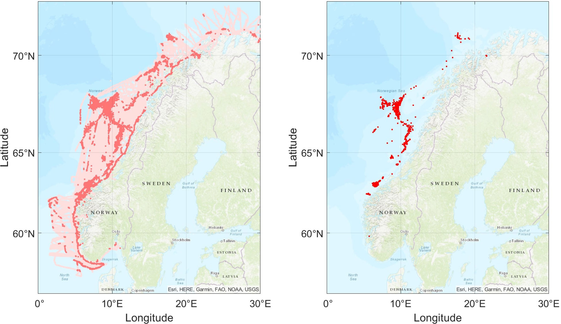
Figure 1 Illustration of the coverage of fishing vessels relative to the catch positions recorded in electronic logs. The left panel displays synthetic measurements predicted by the neural network d, with light red points indicating absence and dark red presence. The predictions uses the independent AIS dataset from early January to late February 2020. The panel on the right shows electronically logged catch points for the same period.
In this article we focus on predictions that inform decision-making, mainly strategic and tactical decisions, using model-based estimation. The estimation procedure uses a large array of synthetic measurements (approximately 2000 per day) derived from ANN output to sequentially estimate fish spatial distributions. The migration model simulates the fine-scale movements of Norwegian Spring Spawning Herring (NSSH) using an individual-based model described in Kelly et al. (2022a). The synthetic measurements predicted by the neural network are assimilated with Monte Carlo simulations of the IBM, using an Ensemble Kalman Filter (EnKF) approach developed in Kelly et al. (2023). Data Assimilation involves applying a correction term to model states based on incoming measurements. Assimilating synthetic measurements with IBM output can improve model forecast estimates and thus inform the catch potential of unexplored ocean areas during the fishing season. Results are presented for simulation scenarios of the independent dataset 2020, from an ANN trained on vessel activity data from 2015:2018.
Absent of model corrections, errors in IBM predictions increase during model simulations due to uncertainties in parameterizations, gaps in knowledge and computational limitations. Through assimilation of derived patterns from fisheries data, we intended to improve IBM predictions when data is available. Since the real distribution of fish clearly influences fishing vessels, it is plausible that the movements of the vessels can contain information about the fish distribution. Our hypothesis was that the IBM predictions can be made more accurate by using model corrections based on vessel movements. This represents a novel approach for improving IBM estimates with real-time data sources. Through developments in computational power and data availability, such modelling approaches will improve our ability to estimate key biological processes.
2 Methods
2.1 Description of data, pre-processing and feature selection
Automatic Identification System (AIS) data for 186 vessels was accessed from the Norwegian coast guard for a total of six years from January 2015 to December 2020, covering the Norwegian Exclusive Economic Zone. The sample consisted of vessels primarily targeting NSSH with purse seiners and pelagic trawls, of both coastal and oceanic fleets.
The received records consisted of variable sampling times (average of 10 seconds), and so to standardize records, they were downsampled to regular 10 minute intervals using statistics over that interval. The data included speed over ground, heading, latitude and longitude coordinates and sample time. Noise in data was low pass filtered using a hampel filter, which replaces the central value in the data window with the median if deemed too distant from the median value, in this case three standard deviations for six point (one hour) windows.
The AIS time series were transformed from the original set of features to motion-related features, similar to Arasteh et al. (2020), where the haversine formula was used to calculate the geographical distance between two consecutive points. The speed, acceleration and jerk were calculated from this geographical estimate. The heading and change in heading were taken from the interpolated dataset. Two additional features were calculated over one hour sliding windows, the first being the number of 45 degree segments of a full circle area visited, and the second being the total distance traversed.
The vessel points were grouped in days of the year and assigned to individual model grid cells with 4 km2 resolution, based on geographical coordinates of AIS points. The median of these motion related features in each 4 km2 grid cell were used as the input for the neural network. In addition, the day, month and year were used as temporal features. The latitude and longitude coordinates of each grid cell were used as spatial features. These 13 features were chosen as it was assumed that the time of year, location and motion of vessels is related to the spatial distribution and abundance of NSSH.
Similarly, the electronic catch logs of the selected vessels were accessed through the fishery directorate and daily catch values of NSSH in kg were assigned to model grid cells. In this study, for simplicity, we assign grid cells with no catch record but AIS points zero values. Logbooks lack coverage and resolution to conclude complex spatial patterns of abundance, and there are several modelling methods that combine AIS and logbook data to address this issue (See for example: [Russo et al., 2018; Adibi et al., 2020)]. For this reason, data is assimilated with high observation noise, reflecting the high uncertainty in logbook data. The target output ti was an p × 1 vector storing the min-max normalized catch values of sampled cells, where p is the full list of sampled cells. The cells with AIS point contained the motion, spatial and temporal-based input vi for the ANN, which was a p × q matrix, where q are the 13 features in each cell. Thus, the ANN was built to predict normalized density outputs ai based on viand normalized ti values (Figure 2).
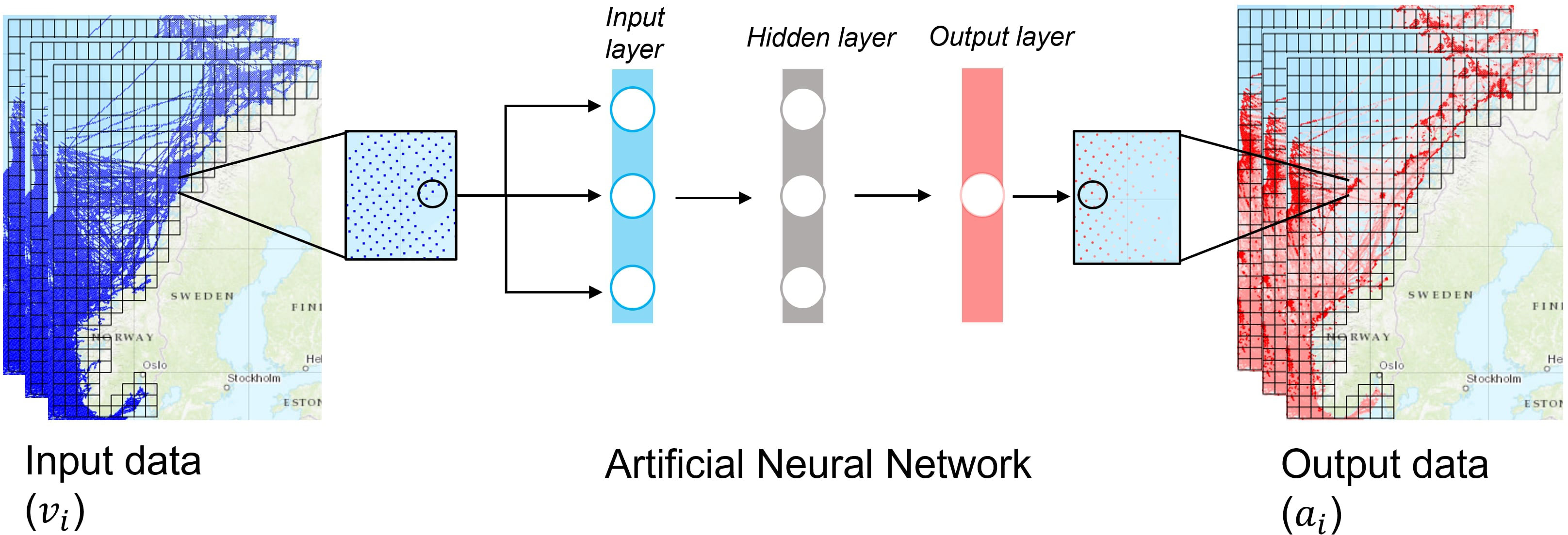
Figure 2 Simplified conceptual illustration of the input of vessel data (vi) passed to the input layer of the shallow ANN which predicted a single output value for the area (ai).
2.2 Synthesizing observations from ANN output data
To generate the synthetic measurements, a shallow feed-forward network was implemented in matlab using nftool. It was chosen given fast computation time and simplicity. Feedfor-ward networks consist of a series of layers, where the first layer has a connection from the network input and each subsequent layer has a connection from the previous layer, before the final layer produces the network’s output. In this case, one hidden layer was used. The process of training a neural network involves tuning the values of the weights and biases of the network to optimize network performance. The input matrix vi for training consisted of over two million data points from 2015:2018. The ANN optimizes weights on parameters to minimize mean-squared normalized errors between the target outputs ti and network outputs ai:
where d is the p × 1 vector of synthetic measurements that were a function of the ANN output data ai and normalized target output ti. Following minimization of the objective F, the function f uses a threshold to determine ai values classified as presence of fish. We calibrated the top 10% of percentiles as the threshold, where above this value a Gaussian random number is selected for d with mean and standard deviation based on ti (Figure 3). Below the percentile threshold, d was treated as absence of fish with a value of zero. The transformation from a to d was based on the assumption that the filter can’t really distinguish between high and low presence values, and furthermore, we needed a way to map filter outputs to reasonable values for model corrections. This is why we used a standard value perturbed with random Gaussian measurement noise. The d vector was calculated for the model simulation period of 15.01.2020 - 28.02.2020 and was assimilated with model forecast estimates in the same period and locations.

Figure 3 Histogram of synthetic non-zero measurement values distribution (d > 0).
2.3 Assimilation with model data
The forecast model used to predict fish densities was an individual-based model of the NSSH spawning migration, described in Kelly et al. (2022a). It was used to model the interaction between conglomerates of individuals (super-individuals) and their surrounding environment. The migration is initialized in northern Norway and progresses south along the Norwegian coast. We present a simplified version of the model for completeness:
where θ is the orientation of the superindividual, calculated based on ∇T and ∇D, the temperature and bathymetry gradients. The intended swimming speed is r, which drives the intended velocity vector vb is balanced with a counter-current response vc. The position state variable p of each individual is updated based on the time step Δt and these two velocity components. The biomass b is updated based on a parameter ω, which reduces biomass by a fixed fraction each Δt.
For the purpose of assimilation with the EnKF, we require a Monte Carlo simulation of the forecast model states to represent the probability distribution. Simply, we initialized N instances of the IBM and added N disturbances α and β to p and b following each time step of the IBM above, described fully in Kelly et al. (2023):
where Xf is the forecast estimate for the assimilation procedure. The function maps from continuous IBM states P and B to the discrete grid representation Xf, which is an n × N density field where each grid cell index n represents the density of fish in a 4 km2 grid cell.
For the calculation of the Kalman Gain K, which is used to calculate the correction term, the covariance of the forecast matrix Xf must be calculated. However, as in many applications, the n × n size is too large to explicitly calculate in the standard EnKF and so an equivalent representation from Mandel (2006) is used instead:
where H is an m × n matrix that maps between model states and measured states, Im is an m × m identity matrix, R is the m × m observation error covariance matrix, where each element on the diagonal is the variance of observation noise (Ω). The parameter Ω is important as it determines the strength of the final correction value. L is an m × N localization matrix which adds a penalty to model covariances that are distant from the measurement points. For a small ensemble and high dimensional system, localization is necessary to limit the impact of spurious correlations in the ensemble (Houtekamer and Mitchell, 2005).
One issue with using observations of fish densities is the non-negative nature of measurement values in d. Observations are usually perturbed with Gaussian noise, but this causes instabilities in the IBM where there are low fish densities. For statistical consistency, this requires a reformulation of the EnKF, and we use the variant known as the deterministic EnKF (Sakov and Oke, 2008):
where d is the vector of synthetic measurements at the time of simulation and H maps m model states in corresponding 4 km2 grid cell. Corrections are applied to each model state and the analysis estimate Xa is the best prediction of posterior model states.
2.4 Analysis
To assess the sensitivity of the model to assimilation of synthetic measurement vector d, our analysis varied two key parameters. The first is r, the intended swimming speed of super-individuals in the IBM (Equations 3). This has a large effect on the rate of progression of the migration southwards along the Norwegian coast. The second parameter varied was Ω, which determines the strength of model corrections through R in Equations 5. Higher Ω value limits the impact of corrections measurements relative to lower Ω values. Control scenarios were simulated with no assimilation of synthetic measurements and thus no Ω values, but with separate realizations of r. By varying r in the control scenarios, overlap that is due to model fit can be separated from the effect of model corrections.
To assess the performance of the various scenarios above, spatial indices were used similar to in Kelly et al. (2023). These are coarse indices, but offer good insight on performance of model scenarios. We calculated the latitude and longitude for each analyzed state , denoted and . The weighted mean or center of gravity of the latitude and longitude are denoted and , while the inertia γ a is a measure of spatial variance of the model:
To measure the overlap κ between the model and observation, spatial indices of catch values were calculated. The weighted geographic mean of catch positions on each day labeled and and the inertia for catch γ t was calculated as above, although instead of , catch weight was used, and the n states were the list of logged catches for the day indexed. A measure of overlap κ between model and catch distribution was calculated:
where a value of zero indicates populations concentrated at two distinct points with no overlap, and a value of 1 indicates perfect overlap. The κ metric was calculated daily for duration of the model simulations and the average value was used to compare different model scenarios (Figure 4).
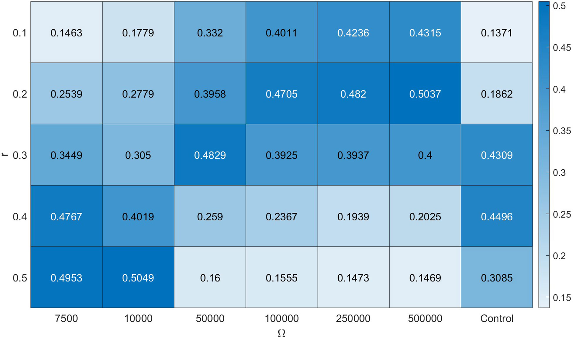
Figure 4 Average κ values, a measure of overlap, for simulation scenarios, with rows representing different r values (swimming speed parameter) and columns representing different Ω values (observation noise). The control scenario was run without assimilation.
For assessing catch potential, we used an index that measured occurrence of catches in areas with model predictions of presence. For this assessment we mapped both the model estimates and the catch locations to a coarser grid of approximately 55km2 ICES statistical rectangles covering the major fishing areas for NSSH in the spring season. A total of 280 grid cells were used, with model presence calculated based on the top 10% of grid cells, and observation presence assigned in cells with at least one catch point. Each day this equaled 28 cells that were assigned model presence, with varying numbers of observation cells assigned presence (Figures 5, 6). The performance of models were calculated as the percentage of observation cells correctly predicted with presence by the model over the simulation period. We compared model predictions to an ensemble of 1000 random strategies, where 28 cells were picked at random each day.

Figure 5 Illustration of catch potential calculated from for different Ω values and a control scenario, where r = 0.2 from 30th of January 2020 to 3rd of February 2020. The black points are the NSSH catch locations during this period. The red squares show the top 10% of model cell values. Note that catch potential estimates in Figure 9 were calculated daily.

Figure 6 Illustration of catch potential calculated from for different Ω values and a control scenario, where r = 0.4 for 19th of February 2020 to 23rd of February 2020. The black points are the NSSH catch locations during this period. The red squares show the top 10% of model cell values. Note that catch potential estimates in Figure 9 were calculated daily.
3 Results
3.1 Sensitivity analysis
Corrections had an effect on the spatial distribution of the 35 scenarios (Figure 4). Lower Ω values pulled several scenarios towards the catch distribution, dependent on the r values. In general, scenarios with r values from 0.1 to 0.3 and higher uncertainty led to higher κ values. For the control scenarios, the highest κ values are achieved for r = 0.3 and r = 0.4, which were within range of the parameter value optimized in Kelly et al. (2022a). Corrections with higher r perform better for lower Ω values. The variability in κ values reflects the fact that different model scenarios experience different sets of measurements throughout the simulation.
Visually, the effect of corrections on the model and for each time step (4 hour increments), we see that with low Ω all corrected models are pulled towards a similar centre point throughout the simulation (Figure 7). Contrasting, with an Ω an order of magnitude higher, the divergence between model states is maintained even with corrections, but there is still a visible effect of corrections (Figure 8). This indicates that different model scenarios converge on similar geographical distributions when there is less uncertainty in measurement values and vice versa.
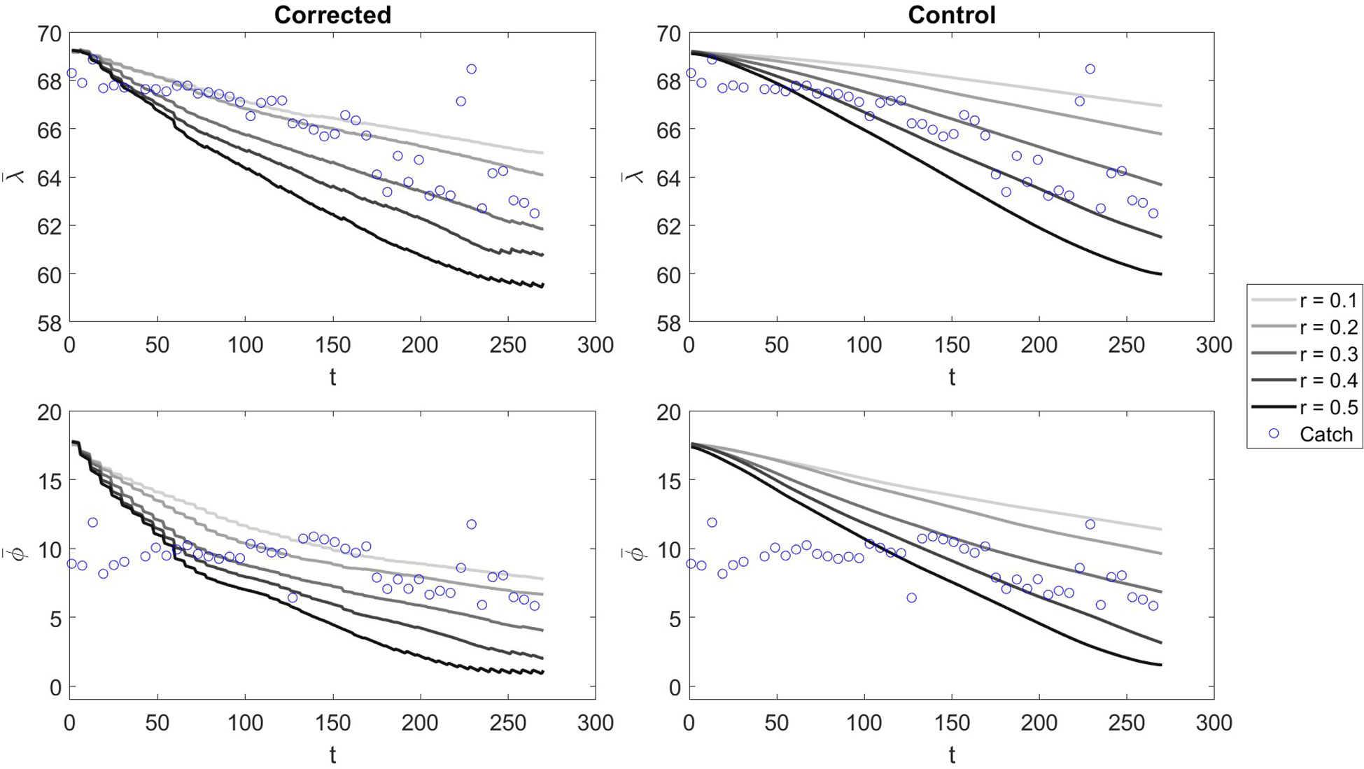
Figure 7 The and values at each time step t of the model run for Ω = 10000 in corrected and control scenarios with varying values of r. The blue bubbles represent the centre of gravity catch values calculated at daily increments.
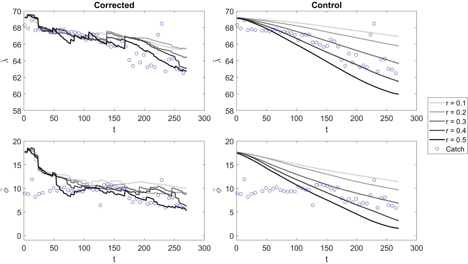
Figure 8 The and values at each time step t of the model run for Ω = 100000 in corrected and control scenarios with varying values of r. The blue bubbles represent the centre of gravity catch values calculated at daily increments.
3.2 Catch potential
The 35 scenarios were compared on the catch potential metric (Figure 9). A random strategy of picking 10% of the cells in the observation area for each day was simulated 1000 times and shown to have an average catch potential of 10%, with a standard deviation of 2%. All model simulations performed better than the random strategy, with lower r values showing the best results on average. At lower levels of Ω, the predicted catch potential was higher than the control performance in every case of r. This indicates that the raw values are imbalanced when comparing κ values as in Figure 4, but filtering values for catch potential improves the capacity to use model-based estimation for decision support.

Figure 9 Catch potential (%) calculated for all model scenarios, with rows representing different r values and columns representing different Ω values and the control scenario without assimilation. For the 1000 random simulations µ = 10% and σ = 2%.
The visualizations of the catch potential in ICES grid cells display how corrected models converge on similar spatial distributions compared to controls (Figures 5, 6). The visualizations are averaged over 5 day periods to increase the number of catch points visualized. In general, the distribution of presence cells becomes more concentrated in corrected output.
When the migration speed is slower, corrections can pull the model forward (Figure 5), while when the model migration is progressing faster, the model can be pulled back with corrections (Figure 6).
4 Discussion
The assimilation approach presented in this article utilized vessel movement data to generate synthetic measurements using a neural network, providing a large array of measurements, predicting both absence and presence of fish, with which to correct model states. Given assimilated scenarios only have access to synthetic measurements in d trained on independent datasets, with no direct information on catches, this illustrates the power of using assimilation of indirect synthetic data to improve model predictions. The final filtering of model output has immediate utility in informing fishing activity.
However, scaling synthetic measurements according to neural network output a loses connection to absolute densities of fish. Further work is required to build a more accurate filter that can predict absolute values. For example, labeling activity along trajectories provides more refined information on vessel behavior such as searching, steaming, pumping and fishing, and these features can improve predictions of densities (Adibi et al., 2020). Additionally, we exclusively used catch logs of NSSH in the ANN, but adding multispecies information on distribution of competitors, predators and prey may also improve predictions. The shallow ANN developed is a proof-of-concept for a more complex system of pattern recognition for complimenting modelling efforts.
We have shown that the model estimates can be strengthened with assimilation, but given we have incomplete knowledge of fish dynamics, scaling errors and other sources of uncertainty, it is challenging to relate predictions to real processes. For the pragmatic purpose of predicting catch potential, this is not a major issue, but when using such a model to test theoretical considerations in ecology, including additional individual states and parameters may be required. Regardless, the Data Assimilation procedure gives insight into the state and parameter values that better fit observations, so if models accurately represent real biological states and parameters, assimilation can sequentially estimate true dynamics in nature.
As Data Assimilation is sequentially estimating model states, it’s challenging to extract the effects of individual corrections. Further work may look more closely at the local effects of assimilation on posterior states. Understanding these effects may reveal how to mitigate some of the instabilities that cause variability in spatial patterns demonstrated in Figure 4. Instabilities in the κ values compared to catch potential metric in Figure 9 shows that when we filter patterns from the model, the predictions become more useful.
The occurrence-based metric for catch potential shows that assimilated models perform well in comparison to control scenarios. Additionally, many weak models perform well under this metric compared to randomly selecting fishing areas. This illustrates the power of extracting simple patterns from model outputs for decision support. Further analysis of spatial patterns may uncover ways in which model output can be filtered for useful input to decision support.
More work is needed to understand what fishers require to reduce search for fishing grounds. There are many factors beyond fish spatial distributions that influence decisions on when and where to fish (Kelly et al., 2022b). Understanding what fishers need from research as well as testing model output in real fishing operations can give insight into how we may inform catch potential. For example, control experiments may be developed where sets of decisions are made with and without model suggestions and analyzed.
Productivity gains from technological innovations in the fishing industry are often countered by a concordant reduction in fish resources (Hannesson et al., 2010). For example, the collapse of the Norwegian herring fishery in the 1970s is attributed to the cumulative impact of new technologies, especially advances in mechanical hauling (Fiksen and Slotte, 2002; Gordon and Hannesson, 2015). Therefore, fisheries management plays a crucial role in avoiding overexploitation of fish stocks. The Norwegian regulatory cycle involves international negotiations, regulatory meetings at the Norwegian fisheries directorate and advice from scientific organizations such as the ICES (Gullestad et al., 2017). Model estimates are a supplementary information source and should thus be utilized in accordance with Norwegian fisheries policy.
5 Conclusion
The model-based estimation system presented in this article is useful in predicting catch potential of novel fishing areas. It relies on a IBM of the herring migration as the forecast estimate and an EnKF procedure is used to correct the estimate based on incoming measurements. We have suggested a simple method for translating vessel activity into synthetic measurements that can be used for assimilation. This is a proof-of-concept for a system to derive patterns for assimilation with model data when direct measurements are unavailable. Data Assimilation produces a posterior field that can be used to predict the spatial distribution of herring. The corrected model forecasts outperform uncorrected forecast estimates when model output is converted to a catch potential metric, especially when the uncorrected forecast estimate are inaccurate. All model estimates perform better than picking fishing grounds at random. Further work can refine the ANN predictions, assess false positive rates in estimates and analyze the utility of the model-based estimation system in decision support.
Data availability statement
The data analyzed in this study is subject to the following licenses/restrictions: AIS data was granted on request from the Norwegian Coastal Authority for the vessel data used in the study. Requests to access these datasets should be directed to https://www.kystverket.no/.
Author contributions
CK: wrote the manuscript and ran simulations. FM: gave feedback on the manuscript. MA: helped setup simulations and gave feedback on the manuscript. All authors contributed to the article and approved the submitted version.
Funding
The work is part of the FishGuider project, which is funded by the project participants and the Norwegian Research Council (project number 296321).
Acknowledgments
We thank the Norwegian Coastal Authority who provided access to the data needed for this study. We greatly acknowledge the support, input and feedback from the project participants: NTNU, SINTEF, NAIS and UiB.
Conflict of interest
The authors declare that the research was conducted in the absence of any commercial or financial relationships that could be construed as a potential conflict of interest.
Publisher’s note
All claims expressed in this article are solely those of the authors and do not necessarily represent those of their affiliated organizations, or those of the publisher, the editors and the reviewers. Any product that may be evaluated in this article, or claim that may be made by its manufacturer, is not guaranteed or endorsed by the publisher.
References
Adibi P., Pranovi F., Raffaetà A., Russo E., Silvestri C., Simeoni M., et al. (2020). “Predicting fishing effort and catch using semantic trajectories and machine learning,” in Multiple-aspect analysis of semantic trajectories. Eds. Tserpes K., Renso C., Matwin S. (Cham: Springer International Publishing), 83–99.
Arasteh S., Tayebi M. A., Zohrevand Z., Glässer U., Shahir A. Y., Saeedi P., et al. (2020). Fishing vessels activity detection from longitudinal AIS data. In proceedings of the 28th international conference on advances in geographic information systems (Seattle WA USA: ACM), 347–356. doi: 10.1145/3397536.3422267
Bal Bes¸ikçi E., Arslan O., Turan O., Ölçer A. (2016). An artificial neural network based decision support system for energy efficient ship operations. Comput. Operations Res. 66, 393–401. doi: 10.1016/j.cor.2015.04.004
Béné C., Barange M., Subasinghe R., Pinstrup-Andersen P., Merino G., Hemre G.-I., et al. (2015). Feeding 9 billion by 2050 – Putting fish back on the menu. Food Secur. 7, 261–274. doi: 10.1007/s12571-015-0427-z
Beveridge M. C. M., Thilsted S. H., Phillips M. J., Metian M., Troell M., Hall S. J. (2013). Meeting the food and nutrition needs of the poor: the role of fish and the opportunities and challenges emerging from the rise of aquaculture a. J. Fish Biol. 83, 1067–1084. doi: 10.1111/jfb.12187
Bez N., Walker E., Gaertner D., Rivoirard J., Gaspar P. (2011). Fishing activity of tuna purse seiners estimated from vessel monitoring system (VMS) data. Can. J. Fish. Aquat. Sci. 68, 1998–2010. doi: 10.1139/f2011-114
de Souza E. N., Boerder K., Matwin S., Worm B. (2016). Improving fishing pattern detection from satellite AIS using data mining and machine learning. PloS One 11, e0158248. doi: 10.1371/journal.pone.0158248
Fiksen Ø., Slotte A. (2002). Stock-environment recruitment models for norwegian spring spawning herring (Clupea harengus). Can. J. Fisheries Aquat. Sci. 59, 211–217. doi: 10.1139/f02-002
Gordon D. V., Hannesson R. (2015). The norwegian winter herring fishery: A story of technological progress and stock collapse. Land Economics 91, 362–385. doi: 10.3368/le.91.2.362
Granado I., Hernando L., Galparsoro I., Gabiña G., Groba C., Prellezo R., et al. (2021). Towards a framework for fishing route optimization decision support systems: Review of the state-of-the-art and challenges. J. Cleaner Production 320, 128661. doi: 10.1016/j.jclepro.2021.128661
Grimm V., Railsback S. F. (2012). Pattern-oriented modelling: a ‘multi-scope’ for predictive systems ecology. Philos. Trans. R. Soc. B: Biol. Sci. 367, 298–310. doi: 10.1098/rstb.2011.0180
Gullestad P., Abotnes A. M., Bakke G., Skern-Mauritzen M., Nedreaas K., Søvik G. (2017). Towards ecosystem-based fisheries management in Norway – Practical tools for keeping track of relevant issues and prioritising management efforts. Mar. Policy 77, 104–110. doi: 10.1016/j.marpol.2016.11.032
Hannesson R., Salvanes K. G., Squires D. (2010). Technological change and the tragedy of the commons: the lofoten fishery over 130 years. Land Economics 86, 746–765. doi: 10.3368/le.86.4.746
Hobday A. J., Spillman C. M., Paige Eveson J., Hartog J. R. (2016). Seasonal forecasting for decision support in marine fisheries and aquaculture. Fisheries Oceanography 25, 45–56. doi: 10.1111/fog.12083
Houtekamer P., Mitchell H. L. (2005). Ensemble kalman filtering. Q. J. R. Meteorol. Soc 131, 3269–3289. doi: 10.1256/qj.05.135
Iglesias A., Dafonte C., Arcay B., Cotos J. (2007). Integration of remote sensing techniques and connectionist models for decision support in fishing catches. Environ. Model. Software 22, 862–870. doi: 10.1016/j.envsoft.2006.05.017
Kelly C., Michelsen F. A., Alver M. O. (2023). An ensemble modelling approach for spatiotemporally explicit estimation of fish distributions using data assimilation. Fisheries Res. 261, 106624. doi: 10.1016/j.fishres.2023.106624
Kelly C., Michelsen F. A., Kolding J., Alver M. O. (2022a). Tuning and development of an individual-based model of the herring spawning migration. Front. Mar. Sci. 8. doi: 10.3389/fmars.2021.754476
Kelly C., Michelsen F. A., Reite K. J., Kolding J., Varpe Ø., Berset A. P., et al. (2022b). Capturing big fisheries data: Integrating fishers’ knowledge in a web-based decision support tool. Front. Mar. Sci. 9. doi: 10.3389/fmars.2022.1051879
Mandel J. (2006). Efficient implementation of the ensemble Kalman filter. Technical Report. University of Colorado at Denver and Health Sciences Center.
Parker R. W. R., Blanchard J. L., Gardner C., Green B. S., Hartmann K., Tyedmers P. H., et al. (2018). Fuel use and greenhouse gas emissions of world fisheries. Nat. Climate Change 8, 333–337. doi: 10.1038/s41558-018-0117-x
Parker R. W. R., Tyedmers P. H. (2015). Fuel consumption of global fishing fleets: current understanding and knowledge gaps. Fish Fisheries 16, 684–696. doi: 10.1111/faf.12087
Pelletier N., André J., Charef A., Damalas D., Green B., Parker R., et al. (2014). Energy prices and seafood security. Global Environ. Change 24, 30–41. doi: 10.1016/j.gloenvcha.2013.11.014
Pennino M. G., Conesa D., López-Quílez A., Muñoz F., Fernández A., Bellido J. M. (2016). Fishery-dependent and -independent data lead to consistent estimations of essential habitats. ICES J. Mar. Sci. 73, 2302–2310. doi: 10.1093/icesjms/fsw062
Reite K.-J., Fernandes J. A., Uriondo Z., Quincoces I. (2021a). “The potential of big data for improving pelagic fisheries sustainability,” in Big data in bioeconomy. Eds. Södergård C., Mildorf T., Habyarimana E., Berre A. J., Fernandes J. A., Zinke-Wehlmann C. (Cham: Springer International Publishing), 371–376. doi: 10.1007/978-3-030-71069-9_28
Reite K.-J., Haugen J., Michelsen F., Aarsæther K. (2021b). Sustainable and added value small pelagics fisheries pilots. Big Data Bioeconomy: Results Eur. DataBio Project 389, 389–409. doi: 10.1007/978-3-030-71069-9_30
Russo T., Morello E., Parisi A., Scarcella G., Angelini S., Labanchi L., et al. (2018). A model combining landings and vms data to estimate landings by fishing ground and harbor. Fisheries Res. 199, 218–230. doi: 10.1016/j.fishres.2017.11.002
Sakov P., Oke P. R. (2008). A deterministic formulation of the ensemble Kalman filter: an alternative to ensemble square root filters. Tellus A: Dynamic Meteorology Oceanography 60, 361. doi: 10.1111/j.1600-0870.2007.00299.x
Schau E. M., Ellingsen H., Endal A., Aanondsen S. A. (2009). Energy consumption in the Norwegian fisheries. J. Cleaner Production 17, 325–334. doi: 10.1016/j.jclepro.2008.08.015
Keywords: neural network, synthetic measurements, individual-based model, ensemble Kalman filter, data assimilation, catch potential
Citation: Kelly C, Michelsen FA and Alver MO (2023) Estimation of fish catch potential using assimilation of synthetic measurements with an individual-based model. Front. Mar. Sci. 10:1171641. doi: 10.3389/fmars.2023.1171641
Received: 22 February 2023; Accepted: 09 October 2023;
Published: 02 November 2023.
Edited by:
Kim J. N. Scherrer, University of Bergen, NorwayReviewed by:
Jin Gao, Memorial University of Newfoundland, CanadaTommaso Russo, University of Rome Tor Vergata, Italy
Copyright © 2023 Kelly, Michelsen and Alver. This is an open-access article distributed under the terms of the Creative Commons Attribution License (CC BY). The use, distribution or reproduction in other forums is permitted, provided the original author(s) and the copyright owner(s) are credited and that the original publication in this journal is cited, in accordance with accepted academic practice. No use, distribution or reproduction is permitted which does not comply with these terms.
*Correspondence: Cian Kelly, Y2lhbi5rZWxseUBudG51Lm5v