Spatiotemporal variations of the oxycline and its response to subduction events in the Arabian Sea

The Arabian Sea is a significant hypoxic region in world’s oceans, characterized by the most extensive oxygen minimum zones (OMZs). Both physical and biological processes can alter the vertical and horizontal distribution of dissolved oxygen within the upper ocean and affect the spatial and temporal distribution of hypoxia within the OMZ. To identify the key physical and biological factors influencing the boundaries of oxycline, we analyzed an extensive dataset collected from the biogeochemical-Argo (BGC-Argo) floats during the period of 2010–2022. In particular, we investigated the impact of physical subduction events on the oxycline. Our results shows that the upper boundary of the oxycline deepened in summer and winter, and seemed to be controlled by the mixed layer depth. In contrast, it was shallower during spring and autumn, mainly regulated by the deep chlorophyll maximum. The lower boundary of the oxycline in the western Arabian Sea was predominantly controlled by regional upwelling and downwelling, as well as Rossby waves in the eastern Arabian Sea. Subduction patches originated from the Arabian Sea High Salinity Water (ASHSW) were observed from the BGC-Argo data, which were found to deepen the lower boundary of the oxycline, and increase the oxygen inventory within the oxycline by 8.3%, leading to a partial decrease in hypoxia levels.

1 Introduction

Dissolved oxygen (DO) is crucial for the survival of marine organisms and it serves as a significant tracer in the ocean (Boyer et al., 1999). Its distribution is influenced by both physical and biogeochemical processes (Garcia, 2005). Prolonged imbalances between oxygen consumption and production can lead to hypoxia, a condition in which the levels of DO are insufficient to support marine life (Schmidtko et al., 2017). The hypoxia zones in the world’s oceans is increasing, which has drawn worldwide attention and prompted significant scientific research efforts (Ulloa et al., 2012; Cavan et al., 2017; Laffoley and Baxter, 2019; Rixen et al., 2020).

The oxygen minimum zone (OMZ) is a layer of low oxygen in intermediate waters that has expanded remarkably in recent years (Stramma et al., 2008; Keeling et al., 2010). Hypoxia is generally defined if the oxygen concentration goes below 60 µmol/kg (Gilly et al., 2013). More than 700 hypoxic zones have been identified in the world’s oceans, primarily in coastal waters and upwelling regions of the Pacific, Atlantic and Indian oceans (Laffoley and Baxter, 2019). The three main permanent OMZs of the world are the Eastern Tropical North Pacific (ETNP), the Eastern Subtropical South Pacific (ETSP), and the North Indian Ocean (NIO) comprising the Arabian Sea (AS) and the Bay of Bengal (BoB). Although hypoxic systems also appear off the Canary and the Benguela, the hypoxic conditions are not as intense as the above. In the NIO, the Arabian Sea hosts a perennial OMZ with a nitrite-bearing zone (Banse et al., 2014), while the Bay of Bengal does not undergo denitrification. The NIO accounts for approximately one-third of the global marine nitrogen loss, with a significant portion originating from the Arabian Sea.

The Arabian Sea is partially enclosed by the Arabian Peninsula, the Indian Peninsula and the Somali Peninsula (Piontkovski and Al-Oufi, 2015; Piontkovski and Queste, 2016). The southwest monsoon prevails in summer, and the northeast monsoon prevails in winter (Sreenivas et al., 2008; Schmidt et al., 2021). The monsoon climate plays a critical role in the dynamics of oceans, atmosphere and land, setting the Arabian Sea apart from other hypoxic areas. The depth of the OMZ in the Arabian Sea is typically between 100 and 1000 m (Rixen and Ittekkot, 2005) and its extent has been expanding consistently (Rixen et al., 2020), leading to a prominent increasing trend in hypoxia (Piontkovski and Queste, 2016). Many studies have focused on the eastward shift of the OMZ and its driving mechanisms (Naqvi, 1987; Resplandy et al., 2012; Rixen et al., 2020; Sarma et al., 2020), as well as the spatiotemporal variations of the oxycline (Prakash et al., 2012; Prakash et al., 2013; Cavan et al., 2017).

The spatiotemporal variation of the oxycline indicates the extent of dissolved oxygen replenishment in the upper ocean, and is an important indicator of the degree of hypoxia in the OMZ. Over the past five decades, the oxycline in the western Arabian Sea has shoaled significantly, from 165 meters in 1960 to 80 meters in 2010, suggesting that hypoxia is becoming more severe in the region. (Prakash et al., 2013). Prakash et al. (2012) found that in the southeastern Arabian Sea, the depth of the oxycline was ~60–120 m with clear seasonal variability. They also observed that abnormal storm events affected the oxycline. The vertical variation in the oxycline was strongly influenced by physical processes such as changes in the thermocline. However, these studies only used very limited number of BGC-Argo floats and defined the oxycline as a certain oxygen isoline, without clearly describing the variation in the upper and lower boundaries of the oxycline.

Additionally, subduction is a physical process that transports water from surface layer into or below thermocline, carrying carbon and dissolved oxygen to the ocean interior (Chen et al., 2021). Most studies focused on the subduction of mode water caused by large-scale circulation (Bange et al., 2001; Schott and McCreary, 2001; Matear and Hirst, 2003; Paterson et al., 2008; Schmidtko et al., 2017; Lachkar et al., 2018). Recent studies have focused on episodic subduction caused by mesoscale eddies and sub-mesoscale processes (Ito et al., 2017; Laxenaire et al., 2018; Trott et al., 2019). The subduction associated with mesoscale eddies transported nutrients from the surface layer downward, resulting in high productivity in the subsurface layer (Trott et al., 2019). Nevertheless, in the eastern boundary upwelling systems of the Arabian Sea, the subduction of incompletely consumed nutrients below the euphotic zone inhibited the productivity of the surface layer (Gruber et al., 2011). However, these studies did not analyze oxygen transport quantitatively and its effect on the oxycline.

In this study, we collected data from all BGC-Argo floats in the Arabian Sea, and analyzed the spatiotemporal variations of both the upper and lower boundaries of the oxycline as well as the factors that influenced it. We also identified and analyzed the effects of subduction events on the oxycline.

2 Materials and methods

2.1 Data source

Early studies of dissolved oxygen in the Arabian Sea used mainly ship-borne data (Scheffzek et al., 1996; Morrison et al., 1998) consisting of very few observations and sparse sampling. Since 2013, when BGC-Argo floats were first deployed, a large quantity of observed data has been amassed (Figure 1), and studies using BGC-Argo oxygen data have greatly improved our understanding of spatiotemporal changes in dissolved oxygen (Prakash et al., 2012; Prakash et al., 2013; Sarma et al., 2020; Mathew et al., 2021). All BGC-Argo float data used in this study were provided by the Global Data Assembly Center of the Argo program (ftp://ftp.ifremer.fr/ifremer/argo).

FIGURE 1

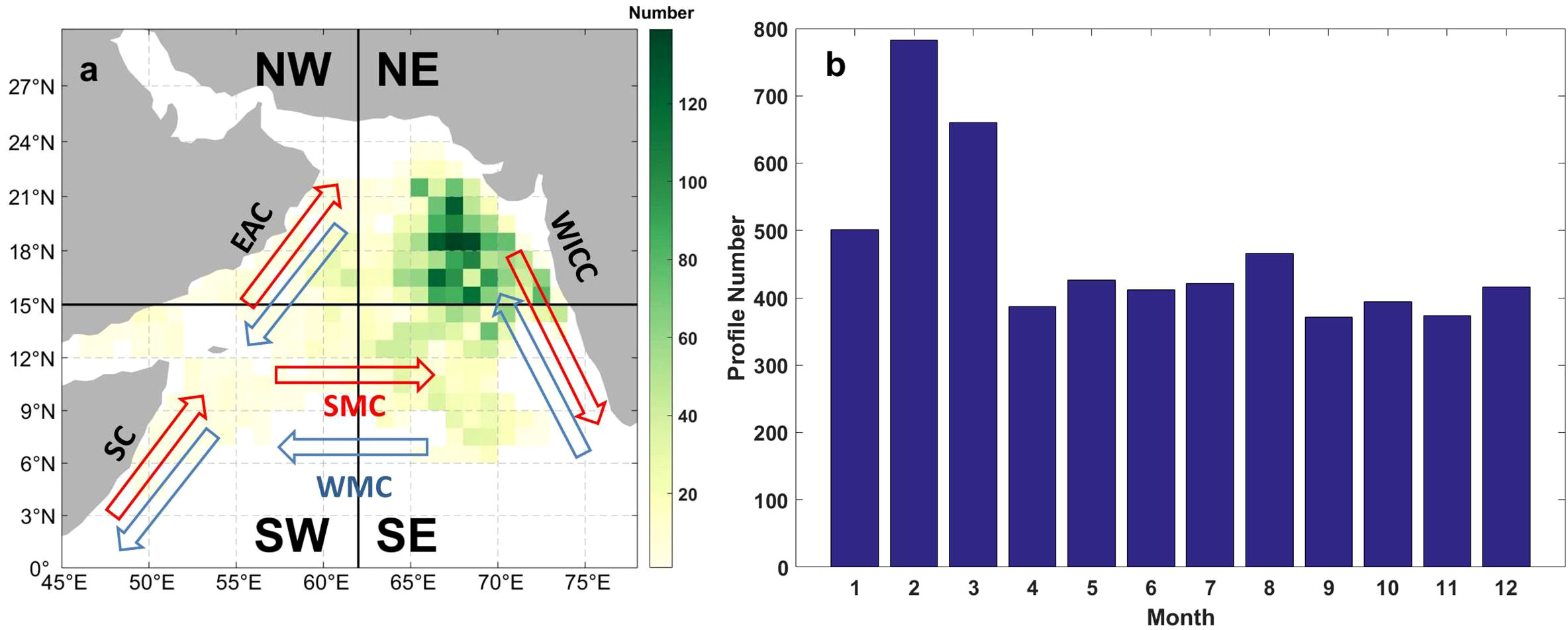
Figure 1 (A) BGC–Argo-observed profile numbers in the 1°×1° grids with the Arabian Sea split into four regions (NE, NW, SE, SW) are shown by the red lines. Red and blue arrows represent the main surface currents in the summer and winter monsoon, respectively. These include the East Arabian Current (EAC), the Somali Current (SC), the Summer Monsoon Current (SMC), the Winter Monsoon Current (WMC), and the Western Indian Coastal Current (WICC); (B) numbers of profiles observed by month.

As of March 2022, 30 floats had been deployed in the Arabian Sea, producing 5561 valid oxygen profiles with approximately 2-m vertical resolution. All oxygen sensor models were Aanderaa 4330/3830 with the accuracy of 8 μmol/kg. Following Sarma et al. (2020), we divided the Arabian Sea into four areas (Figure 1A): Northwest (NW: 15–30°N, 45–62°E), Northeast (NE: 15–30°N, 62–78°E), Southwest (SW: 5–15°N, 45–62°E) and Southeast (SE: 5–15°N, 62–78°E). Such a regionalization is due to the distribution and extent of hypoxia, as well as the influence of surface currents: (1) The most intense hypoxia zone with denitrification appears to the east of 62°E in the AS, as identified in Naqvi (1991); (2) There is larger meridional variability in the lower boundary of the OMZ and deeper OMZ depths in the northern region of >15°N (>1000 m) compared to the southern region (550–1000 m), as shown in Sarma et al. (2020); (3) In the western part of the AS, the East Arabian Current (EAC) primarily influences the north region (>15°N), while the Somali Current (SC) has a stronger impact on the south region (<15°N) (Figure 1A); (4) In the southern part of the AS, the main surface currents, namely the Winter Monsoon Current (WMC) and the Summer Monsoon Current (SMC), predominantly affect the area below 15°N (Figure 1A). Most profiles were distributed in the NE region, where the profile numbers in most grids (1°×1°) were >60. In terms of seasons, about 30.6% of profiles were captured in winter (December–February; 1700), followed by spring (March–May; 1474), summer (June–August; 1299) and autumn (September–November; 1138). The float-observed variables included temperature, salinity, dissolved oxygen and chlorophyll.

2.2 Data processing

Potential density was derived from pressure, temperature and salinity, and mixed layer depth (MLD) was calculated as the depth at which sea water density increased by 0.03 kg/m³ compared to the density at 10 m (de Boyer Montégut et al., 2004). The deep chlorophyll maximum (DCM) depth for each profile, z_DCM, was defined as the depth at which chlorophyll reached the maximum value. If z_DCM was shallower than MLD (i.e., maximum chlorophyll appeared in the mixed layer), the water column was well mixed (i.e., the deep mixing eroded DCM). Dissolved oxygen concentrations were first quality-controlled following Thierry et al. (2021), As shown in Eq. 1, the delayed-mode correction of oxygen data used the climatology-based method of Johnson et al. (2015) and considered the time-dependent drift.

$\begin{array}{ll}{[O_2]}_{cor} = \left\{G_1+(t-t_1)·d\right\}{[O_2]}_{raw}& (1)\end{array}$

Here, [O₂]_raw and [O₂]_cor represent the uncorrected and corrected oxygen data, respectively. G₁ represents the initial gain factor for the first profile, and d represents the time-dependent in-situ drift, t and t₁ are the observing times for a certain profile and the first profile, respectively

The oxycline, which is located below MLD, is defined by the upper depth of the oxycline (UOXL) and the bottom depth of the oxycline (BOXL). These depths are determined based on the vertical gradients (the slope of 5-point linear regression) of the oxygen profile. The UOXL was defined as the depth at which the gradient first became< −1 μmol/kg/m, and the BOXL was defined as the lowest depth at which the gradient was< −1 μmol/kg/m. The gradient criterion (-1 μmol/kg/m) was chosen based on the accuracy of 8 μmol/kg of oxygen sensor, the vertical resolution of 2 m, and the 5-point slope calculation (i.e., the slope was determined in an 8-m layer, where the change in the oxygen concentration that exceeded the sensor accuracy was considered reliable). Monthly averaged sea–surface wind stress and Ekman pumping velocity (EPV) data were observed by the ASCAT sensor on the Metop-A satellite (Hu et al., 2022) and provided by NOAA (https://coastwatch.pfeg.noaa.gov/). The satellite data were for the period October 2009–January 2022 and had a horizontal resolution 0.25°×0.25°.

2.3 Detection method of subduction events

When subduction occurs, surface waters would be transported to subsurface along isopycnals, and a distinct water patch with anomalous physical and biogeochemical properties would appear at depth. These anomalous features can be captured when a BGC-Argo float coincidently passes by. The anomalies of dissolved oxygen and spicity (π; defined as a nearly orthogonal property to density in θ-S diagram) observed from the BGC-Argo profiling were typically used to identify subduction patch(e.g., Llort et al., 2018; Chen et al., 2021). Spicity allows differentiating water masses with distinct thermohaline properties but similar density (a typical subduction signature), and DO is typically used to indicate the biogeochemical properties of a water mass. Following previous studies, thresholds of the anomalies in DO and π are defined to identify a subduction patch. The general detecting steps of subduction patches are as follows (Figure 2).

(1) Calculate the gradients of π and oxygen at each measurement depth.

(2) Find the profile peak based on the calculated gradient profile; when the gradient changes from positive to negative, the point is a negative peak value, and vice versa.

(3) Find the depth at which both π and oxygen showed a peak, and save this depth as a peak_depth.

(4) Select the baseline and calculate Δπ; 200 m was chosen as the reference thickness on the assumption that no subduction event affected >200 m in a profile. If the peak is negative (positive), find the maximum (minimum) value within the depth range from (peak_depth − 100 m) to (peak_depth + 100 m) (green triangles in Figure 2) and set these as the two endpoints of the baseline. Δπ is calculated from the difference between spicity and the baseline.

(5) Calculate ΔDO using the same method, independent of Δπ.

(6) A subduction signal was identified when ΔDO >10 μmol/kg and |Δπ| > 0.05 kg/m³.

FIGURE 2

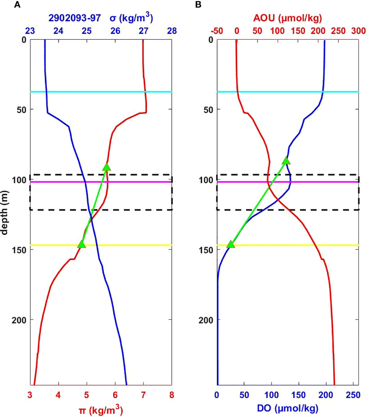
Figure 2 An example of a profile with the subduction signal (profile no. 97 observed by Float 2902093): (A) Potential density (σ, blue solid line) and spicity (π, red solid line); (B) dissolved oxygen (DO, blue solid line) and apparent oxygen utilization (AOU, red solid line). The magenta line represents the depth of the regional maximum values of spicity and oxygen (peak_depth); the green triangles represent maximum value of spicity and oxygen within the depth range from (peak_depth − 200 m) to (peak_depth + 200 m) and the green line represents the baseline connecting the two endpoints. the area within the black dashed lines represents the detected subduction range. The cyan and yellow lines represent the upper depth of the oxycline (UOXL) and the bottom depth of the oxycline (BOXL), respectively.

In order to evaluate the impact of subduction events on the oxycline and OMZ, we calculated the dissolved oxygen inventory using the depth-integrated ΔDO within the subduction signal range as follows.

$\begin{array}{ll}\text{oxygen inventory}={\sum }_{z=p_{lower}}^{z=p_{upper}}\Delta D{O}_z& (2)\end{array}$

Where ΔDO_z is the DO anomaly at depth z, and p_upper and p_lower are the upper and lower boundary depths of the detected subduction signal.

3 Results and discussion

3.1 Physical setting

3.1.1 Seasonal cycles of the mixed layer depth

The mixed layer plays a crucial role in the exchange of both heat and oxygen between the atmosphere and the ocean. (Kumar and Narvekar, 2005; Singh et al., 2019). In the Arabian Sea, the MLD is mainly governed by the monsoon system with seasonal variations. In the NW region (Figure 3A), wind stress was about 0.05 N/m² in spring, and MLD was relatively shallow (20–30 m). Wind stress increased significantly in summer to 0.28 N/m². MLD also deepened accordingly, with a maximum depth of 50 m and an average depth of 40 m. Wind stress and MLD in autumn were similar to the spring levels. Wind stress in winter was in the range 0.05–0.1 N/m². However, MLD reached the greatest depth of 55 m in winter, which was inconsistent with the changes in wind stress. This occurred because the northeast monsoon in winter is a dry and cold continental wind that increases ocean evaporation, associated with heat loss and thus a reduction in sea surface temperature. Vertical mixing intensifies due to the convection effect (Madhupratap et al., 1996; Kumar et al., 2001; Sreenivas et al., 2008; Lachkar et al., 2018). Even so, the correlation between wind stress and MLD was strong (R = 0.76; Figure S1A). In the NE region, average wind stress showed seasonality similar to the NW region but with a lower value in summer. MLD was 35–45 m in summer and 25–40 m in winter (Figure 3B), and the correlation between wind stress and MLD was 0.86 (Figure S1B). Prasanth et al. (2021) found that the MLD was 64 ± 15 m in summer and 56 ± 19 m in winter in the same region. The differences were most likely due to the different methods applied in the calculation of MLD (they calculated MLD as the depth where density equals to the sea surface density plus an increase in density equivalent to a reduction in the temperature of 0.25°C, which was about ~ 5 m deeper than). MLD was deep in both summer and winter in the SW and SE regions (Figures 3C, D), which was consistent with the north region. The correlation coefficients in the two regions were 0.81 and 0.92, respectively (Figures S1C, D). Observed MLD values in these two regions were close to the observations of Sreenivas et al. (2008). Overall, wind stress and MLD changes were very closely synchronized, showing high correlations in all regions. These results suggest that MLD was driven mainly by wind all the year round, although in winter, the convection effect was an important factor in increasing MLD.

FIGURE 3

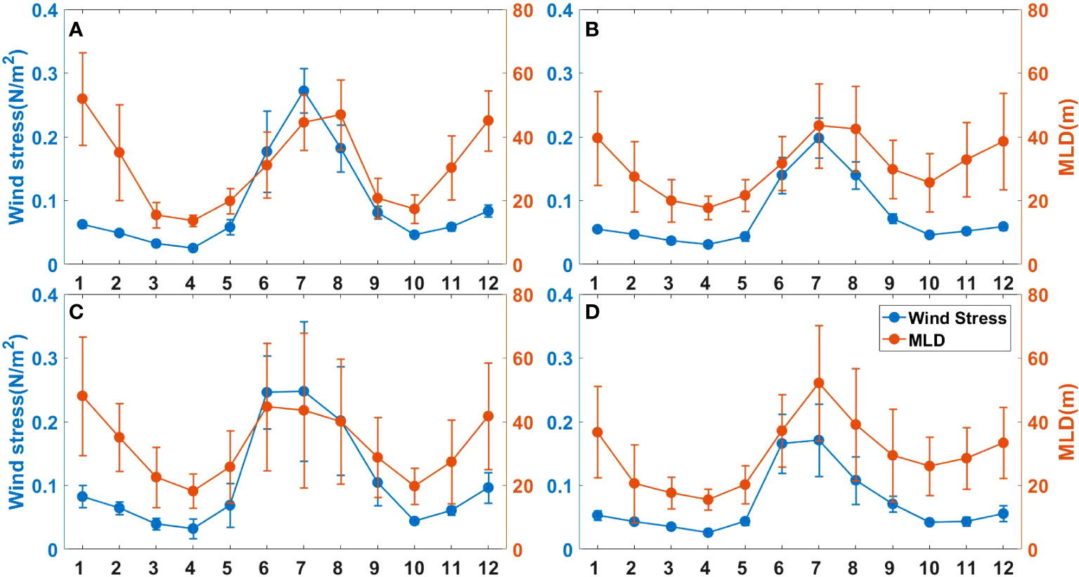
Figure 3 Spatiotemporal variation in wind stress (N/m², blue line) and MLD (m, orange line) by region: (A) NW, (B) NE, (C) SW, (D) SE.

3.1.2 Seasonal cycles of the thermocline

Wind-driven Ekman pumping causes vertical transport of the water mass. Positive EPV corresponds to the upward transportation of seawater (upwelling), and thus the uplift of thermocline and pycnocline and oxycline; conversely, negative EPV corresponds to downward transportation of seawater (downwelling), and the depression of thermocline, pycnocline and oxycline (Williams and Follows, 2003; McCreary et al., 2009; Hu et al., 2022). We selected an isotherm of 21.4°C as the thermocline indicator as this was the temperature closest to the bottom depth of the oxycline in the Arabian Sea.

In the NW region, EPV was approximately −1.5×10⁻⁶ m/s in spring, and the isotherm was located at 120–130 m. In summer, EPV became positive and gradually increased to a maximum in July. The isotherm became correspondingly shallower. In autumn, EPV was positive in September and October but became negative in November; isotherm depth also changed from 90 m to 110 m. In winter, EPV was negative, and isotherm depth increased to a maximum of 130 m in February (Figure 4A). EPV and isotherm were weakly negatively correlated (correlation coefficient as −0.55; Figure S2A); In the NE region, EPV was also negative in spring, and isotherm depth gradually increased from 120 m to 140 m. In summer, EPV abruptly became positive, and the isotherm became shallower. However, during autumn and winter, when EPV again became negative, isotherm depth did not increase (Figure 4B). The correlation coefficient between EPV and isotherm was only −0.12 (Figure S2B); In the SW region, EPV was positive in summer, and the isotherm became shallower (Figure 4C). In other seasons, EPV was closer to 0, and the average isotherm depth was approximately 110 m (Figure 4C). The correlation coefficient between EPV and isotherm was −0.57, and the linear relationship was close to that in the NW region (Figure S2C); In the SE region, EPV was negative in summer, thus differing from other regions, and isotherm depth increased slightly (Figure 4D). EPV was close to 0 in other seasons, and the isotherm was shallower in winter (Figure 4D). The correlation coefficient between EPV and the depth of isotherm 21.4 °C was 0.82 (Figure S2D). Our results were consistent with those of Prakash et al. (2012), who found that in the SE region, the thermocline was highly influenced by Rossby waves, and that westward propagating Rossby waves led to the thermocline shoaling in the early winter. Except in the NE region, EPV and isotherm were negatively correlated. In the western Arabian Sea, upwelling prevailed in summer and downwelling prevailed in winter, leading to considerable changes in the thermocline (Rixen et al., 2020). In the SE region, Rossby waves made the thermocline shallow in October–January and deep in March–September (Ravichandran et al., 2012; Amol, 2018).

FIGURE 4

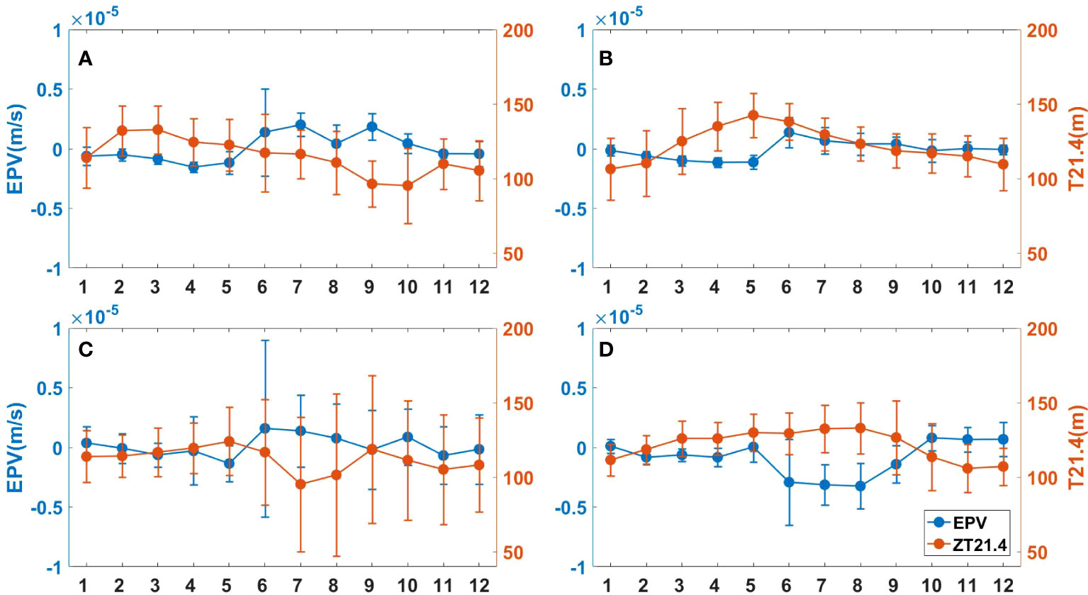
Figure 4 Spatiotemporal variation in EPV (m/s, blue) and isotherm (m, orange) by region: (A) NW, (B) NE, (C) SW, (D) SE.

In general, the Ekman pumping effect was a significant driver of the variations in the isotherm depth, except during the summer monsoon season from June to September, when there was a noticeable mismatch between EPV and isotherm depth in the NW, NE and SE regions. Positive EPV values were observed in both NW and NE regions (Figures S2A, B), and negative EPV in the SE region (Figure S2D); however, the isotherm depth did not respond to these EPV variations in this period. This lack of response in the NW region was likely caused by the insufficient data observations, which limited our understanding of the relationship between EPV and isotherm depth; while in the NE and SE regions, it may be attributed to Rossby waves, which led to a deeper thermocline during summer monsoon and a shallower thermocline during winter monsoon, modulating the relationship between Ekman pumping and the observed thermocline.

3.2 Seasonal cycles of the oxycline and driving factors

3.2.1 Seasonal cycles of the oxycline

In the NW region (Figure 5A), the upper boundary of the oxycline (UOXL) was at 40–50 m depth in spring, close to the DCM depth, and the lower boundary of the oxyline (BOXL) was at 100–150 m depth. In summer, MLD deepened significantly, DCM shoaled and became shallower than MLD in July and August, when the upper layer chlorophyll profile became well mixed and the calculated DCM was influenced by the non-photochemical quenching (NPQ; Xing et al., 2012). UOXL deepened along with MLD, while BOXL shoaled following the isotherm. In autumn, UOXL shoaled along with MLD, BOXL abruptly deepened from October, exceeding 150 m; In winter, UOXL deepened again following MLD, and BOXL shoaled following the isotherm; In the NE region (Figure 5B), UOXL was close to the DCM depth in spring and deepened as MLD deepened in summer, similar to the NW region. In autumn, MLD shoaled but DCM deepened, and UOXL remained below DCM. In winter, UOXL deepened as MLD deepened. BOXL was tightly coupled with the isotherm throughout the year. The observed values of DO and DCM were close to those of Mathew et al. (2021); In the SW region (Figure 5C) in spring, UOXL was very close to DCM, which was deeper than MLD. In summer, MLD deepened rapidly to below DCM; UOXL changed little but remained deeper than MLD. In autumn and winter, UOXL shoaled in October–November and deepened in December–January, corresponding to the changes in MLD. BOXL showed relatively weak seasonal change compared to UOXL, except for shoaling in summer, matching the seasonal behavior of the isotherm; In the SE region (Figure 5D), DCM was generally deeper than MLD, except for July–August, when MLD deepened below DCM. UOXL was deeper than both MLD and DCM, and showed relatively weak seasonal change except for a pronounced deepening in July–August. The observed results for DO and DCM were close to those of Ravichandran et al. (2012).

FIGURE 5

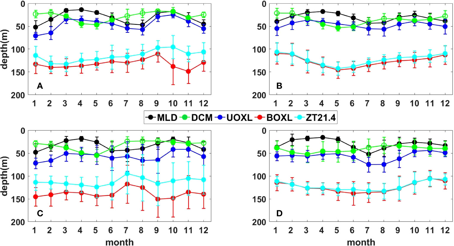
Figure 5 Spatiotemporal variation in UOXL (blue), BOXL (red), MLD (black), DCM (green), and isotherm (cyan) by region: (A) NW, (B) NE, (C) SW, (D) SE.

3.2.2 Driving factors of the oxycline at seasonal scale

Correlation analysis showed that when MLD was deeper than DCM (i.e., in well-mixed water), UOXL was mainly governed by MLD; the correlation coefficient was 0.75 (Figure 6A). When MLD was shallower than DCM (i.e., the water was stratified), UOXL was driven by DCM; the correlation coefficient was 0.63 (Figure 6B). Seasonal dynamics of BOXL were affected by the thermocline (pycnocline); the correlation coefficient between the 21.4°C isotherm and BOXL was 0.82 (Figure 6C).

FIGURE 6

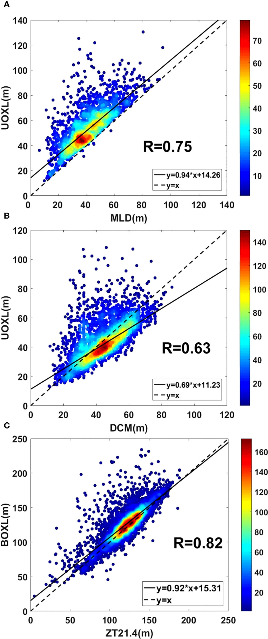
Figure 6 (A) Correlation between MLD and UOXL when MLD was deeper than DCM; (B) correlation between DCM and UOXL when DCM was deeper than MLD; (C) correlation between BOXL and isotherm.

During the spring intermonsoon period, wind speed was low, and solar shortwave radiation was high and reached a maximum in April–May. Surface water was heated and stratification therefore increased (Kumar and Narvekar, 2005), resulting in weak mixing and shallow MLDs. In addition, in the SE region, from February onward, low-salinity water from the Bay of Bengal flowed into the region together with water from the West India Coastal Current (WICC) and the Winter Monsoon Current (WMC) (see Figure 1A; Ravichandran et al., 2012). Phytoplankton productivity was influenced by the decreased mixing and the relatively deep euphotic depth in spring (Ravichandran et al., 2012). The maximum chlorophyll appeared below the mixed layer, which increased oxygen production, thickened the oxic layer and thus deepened UOXL.

In summer, wind speed increased, reaching a maximum of 13 m/s in July (Kumar and Narvekar, 2005), short wave radiation decreased, and thus MLD deepened. At 5°N, a northeast Findlater Jet formed (Prasad et al., 2001) and forced negative (positive) wind stress curl in the SE (NW) area, which intensified mixing (Rixen et al., 2020). In the western region, upwelling occurred along the coasts of Oman and Somalia (Prasad et al., 2001; Rixen et al., 2020) that transported nutrients from the subsurface layer to the surface (Queste et al., 2018) and so promoted chlorophyll production (Brock et al., 1991; Brock and McClain, 1992). Maximum chlorophyll formed in the surface layer (Gundersen et al., 1998). The thickness of oxic layer was highly modulated by the mixed layer, and UOXL thus followed MLD. BOXL rose as upwelling lifted the thermocline. Advection transported nutrients from the NW region to the NE region (Girishkumar et al., 2012; Amol, 2018). Under the combined effects of mixing and thermocline uplift, surface nutrients were replenished and productivity increased (Banse, 1987; Lotliker et al., 2020). In the SE region, BOXL deepened as Rossby wave propagation deepened, and the pattern of MLD and DCM in autumn was similar to that in spring.

During the winter monsoon, vertical mixing intensified due to both wind and convection. Evaporation was greater than precipitation because net heat loss of the ocean to the atmosphere and shortwave radiation had decreased, and so the convective mixing increased (Madhupratap et al., 1996), bringing nutrients to the surface, and thus enhancing surface productivity (Banse, 1987; Kumar et al., 2001; Lotliker et al., 2020). However, in the NE region, the effects of mixing and nutrient transport were limited by the northward and westward inflow of low salinity water (Ravichandran et al., 2012), and the chlorophyll maximum formed below the mixed layer. This phenomenon was different than in other areas, and UOXL was thus close to DCM in the NE region. In the western region, currents were from north to south, and the Ekman transport formed a downwelling, which deepened BOXL.

3.3 Effects of subduction events on the oxycline

3.3.1 Spatiotemporal distributions of subduction events

A total of 159 profiles (2.9% of all observed profiles) were determined to have been influenced by subduction events, based on the detection method described in Section 2.3. The subduction profiles were observed mainly in the NE region. The greatest profile density was 11 per grid (Figure 7A). However, the probability density of subduction profiles in the NE region (the number of identified subduction profiles in a grid square divided by the number of all observed profiles in the entire grid) was not noticeably greater than in the other regions, being<30% (Figure 7B). In terms of monthly distributions (Figure S3), the probability density of subduction profiles was greatest in April (5.7%) and least in December (1.4%); seasonally, most subduction profiles were observed in spring (13.5%).

FIGURE 7

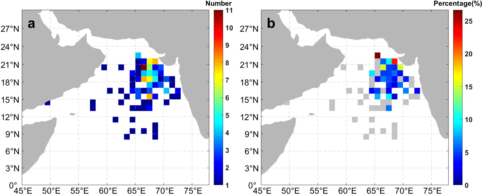
Figure 7 Spatial distribution of (A) subduction profiles and (B) probability density of detected subduction profiles. The grey points in Panel (B) represent the pixels with only one subduction profile.

The depth range of the oxycline in the Arabian Sea was generally from 50 m to 200 m. Most subduction events occurred within the oxycline (57.2%), and a few (10.6%) below the oxycline (i.e., in the OMZ). Subduction events that were identified below the oxycline were distributed in all four regions, but subduction events that occurred within the oxycline were concentrated in the NE region (Figure 8A). Subduction events ventilated oxygen into the subsurface or even intermediate depths. Profiles with abnormal oxygen signals (ΔDO) of 10–30 μmol/kg accounted for 42.8% of all subduction events, and their distribution was very scattered (Figure 8B), which indicated that many weak subduction signals were captured over a considerable distance. Oxygen was exchanged between the subducted water masses and mixed with the surrounding waters. Strong subduction events, with ΔDO of 30–50 μmol/kg and >50 μmol/kg accounted for 36.5% and 20.7% of all subduction events. They were mainly recorded in the NE region (Figure 8B), which suggests that most subduction events originated in this region and also ventilated oxygen into the oxycline in this region.

FIGURE 8

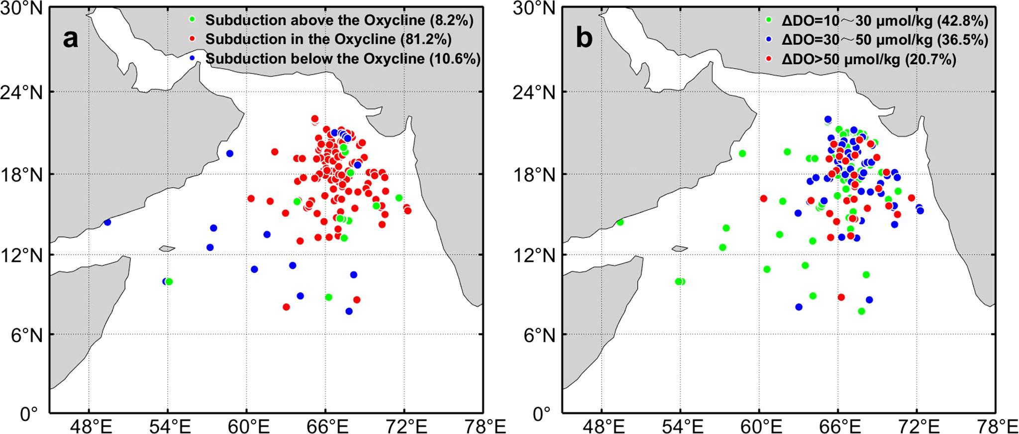
Figure 8 Horizontal distribution of BGC-Argo profiles identifying subduction events: (A) relationship between subduction events and the oxycline: subduction occurred above the oxycline (green dot, 8.2%), within the oxycline (red dot, 81.2%), and below the oxycline (blue dot, 10.6%); (B) the intensity of subduction, as measured by ΔDO: 10–30 μmol/kg (green dot, 42.8%), 30–50 μmol/kg (blue dot, 36.5%), and > 50 μmol/kg (red dot, 20.7%).

Seasonally, most subduction events occurred in spring (41.5%), followed by winter (21.4%), summer (18.9%), and autumn (18.2%). In terms of monthly distribution, most subduction events occurred in March (17.0%), followed by April (13.8%). Subduction events occurred within the oxycline irrespective of month, but above the oxycline only in spring and summer, and below the oxycline (i.e., within OMZ) in every month except June (Figure 9A). Weak subduction events (ΔDO in the range 10–30 μmol/kg) and strong subduction events (ΔDO in the range 30–50 μmol/kg) occurred every month, with the greatest proportion occurring in spring. The proportion of subduction events with ΔDO >50 μmol/kg was also high in spring (Figure 9B), which suggests that oxygen ventilation was greatest in spring. Most subduction events showed high spicity (Δπ ≥0.3 kg/m3; Figure 9C), which indicates that subduction in the Arabian Sea was mainly related to waters with high salinity.

FIGURE 9

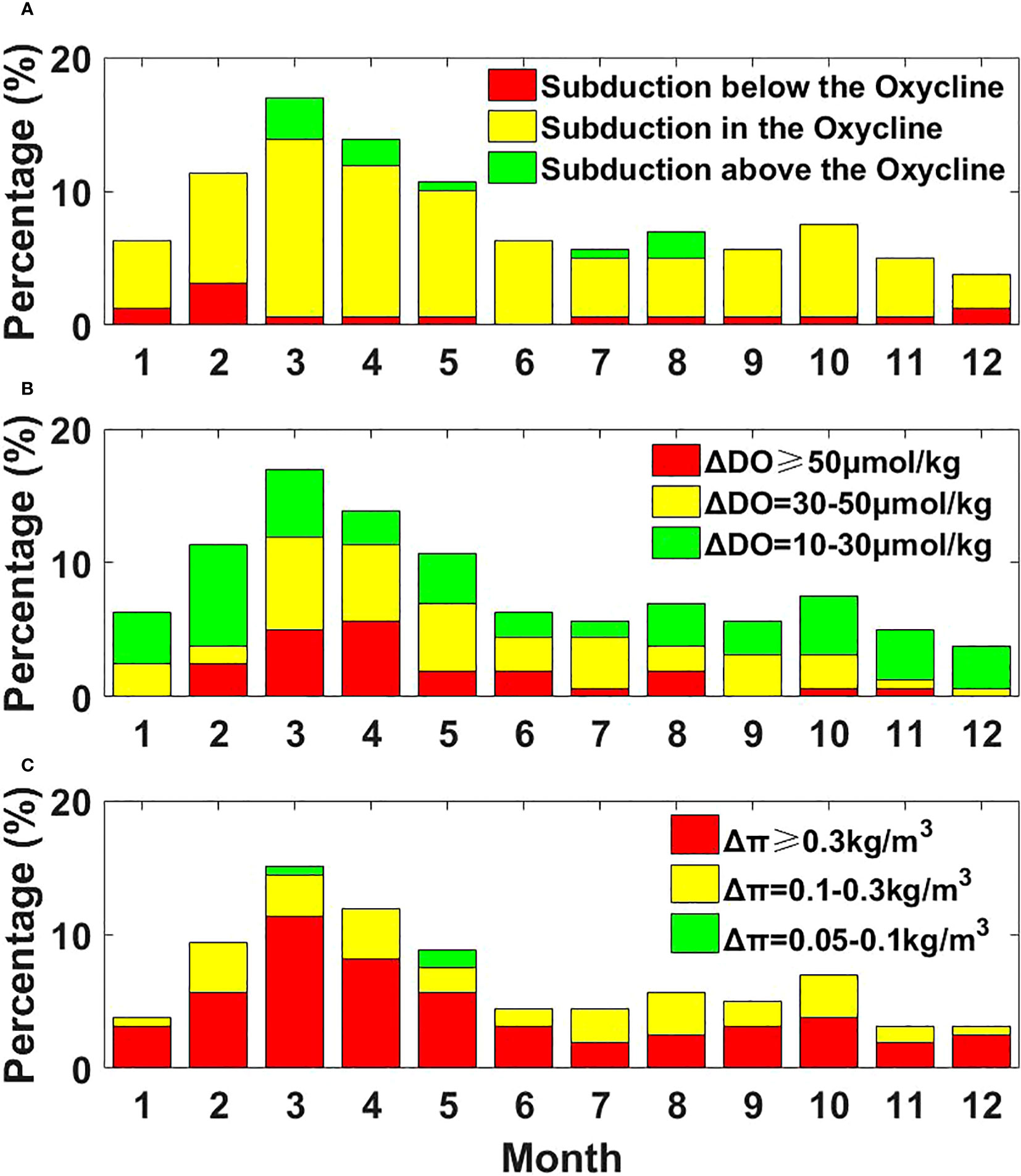
Figure 9 Distributions of subduction events in January–December (A) by depth and (B, C) by intensity (B, C): (A) the proportion of subduction events relative to the oxycline; (A) the proportional distribution of ΔDO at the maximum dissolved oxygen anomaly; (C) the proportional distribution of Δπ at the maximum spicity anomaly.

3.3.2 Origin of subduction events

Water masses with high temperature and high salinity in the Arabian Sea include Persian Gulf Water (PGW), Red Sea Water (RSW), Indian Ocean Central Water (ICW) and Arabian Sea High Salinity Water (ASHSW) (Shetye et al., 1994; Prasad et al., 2001; Ahmed, 2021). PGW formed in the Persian Gulf and flows into the Arabian Sea from the Gulf of Oman at a depth of 200–300 m (Morrison et al., 1999; McCreary et al., 2013). PGW spreads along two paths: southward along the coast of Oman and southeasterly along the coast of India (Acharya and Panigrahi, 2016; Shenoy et al., 2020); there is no evidence that the spreading of PGW is seasonal (Jain et al., 2016). RSW forms in the Red Sea and flows into the Arabian Sea through the Gulf of Aden at a depth of 600–800 m (Beal et al., 2000; Shenoy et al., 2020). RSW spreads south mainly along the coast of Somalia and north along the coast of Oman into the central Arabian Sea (Schmidt et al., 2020). RSW flow is observed primarily in summer (Schmidt et al., 2020). ICW is a mixed water mass derived from Antarctic Intermediate Water, Subantarctic Mode Water, and Indonesian Intermediate Water (Lachkar et al., 2019). ICW flows from south to north and mixes with the Somali current to flow into the Arabian Sea, propagating within a depth of 200–500 m (Schmidt et al., 2020) and extending to 16°N (Shenoy et al., 2020). ASHSW forms in the northern Arabian Sea at a depth of 0–150 m and spreads southward (Kumar et al., 2019).

The temperature and salinity of the maximum spicity anomaly for each subduction-affected profile was plotted in the temperature–salinity (T–S) diagram (Figure 10), shows that the subduction signals were far from PGW, RSW or ICW but close to ASHSW. This characteristic was particularly true for the shallow subduction events (<100 m). ASHSW forms during the winter monsoon period (Banse and Postel, 2009). Evaporation of seawater in the northern Arabian Sea is greater than local precipitation, resulting in an increase in surface salinity. The northeast monsoon is a dry season with cold continental wind, wherein surface seawater loses heat in winter and the intensified convective mixing led to formation of the ASHSW (Kumar and Prasad, 1999; Chowdary et al., 2005). ASHSW is subducted in winter and spring and gradually spread southward (Thadathil et al., 2008). The core ASHSW spreads to 10°N in May, reaches 15°N in the central basin in summer, and returns to 20°N in autumn (Prasad, 2002; Chowdary et al., 2005). The seasonal spreading of ASHSW was consistent with our results, showing that the detected subduction profiles were concentrated in the NE region and had the greatest probability density in spring.

FIGURE 10

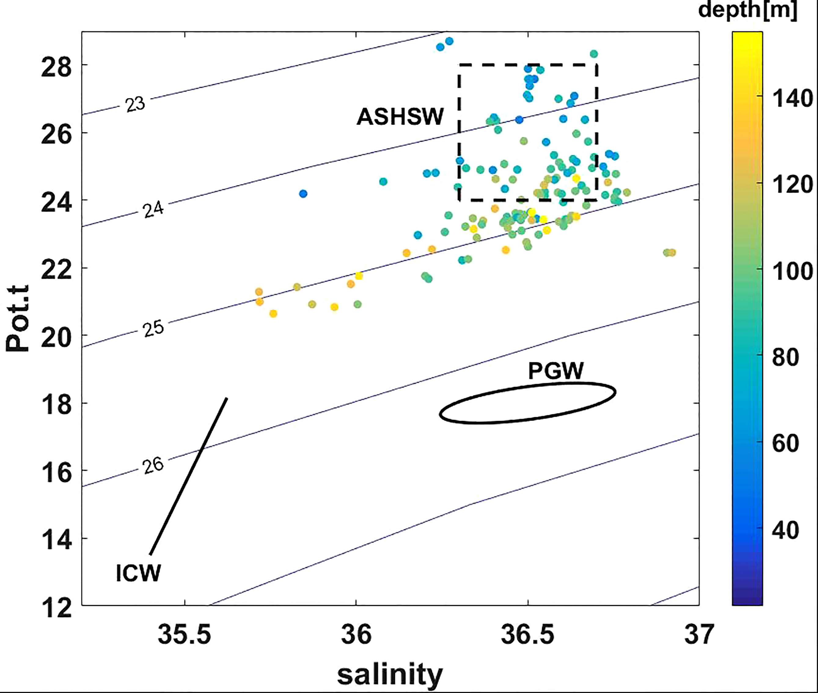
Figure 10 T–S diagram at the maximum spicity anomalies of subduction profiles; the black dashed box indicates the ASHSW range, the black oval indicates the PGW range and the black solid line indicates the ICW range.

3.3.3 Effects of subduction on oxycline

Comparison of the subduction-affected profiles with nearby profiles shows that the subduction events deepened BOXL by 4.6 m but had no obvious effects on MLD or UOXL (Figure 11). The thickness of the subduction occurring in the oxycline was 23.2 ± 16.6 m and it increased the oxygen inventory of the entire oxycline by 8.3 ± 4.5%. The subduction events therefore increased the oxycline thickness and also supplemented oxygen into the oxycline. The subduction thickness in OMZ reached 33.5 ± 25.2 m and increased oxygen in the entire OMZ by 6.4 ± 3.3%. Oxygen ventilation of OMZ was obvious, which suggests that subduction of ASHSW was important in reducing hypoxia in the northeast Arabian Sea. Particularly, the subduction events could break the nitrite bearing zone of the ASOMZ in winter (northeast monsoon) as shown in Shenoy et al. (2020). Thus, oxygen intrusion into the OMZ via subduction kept denitrification in check.

FIGURE 11

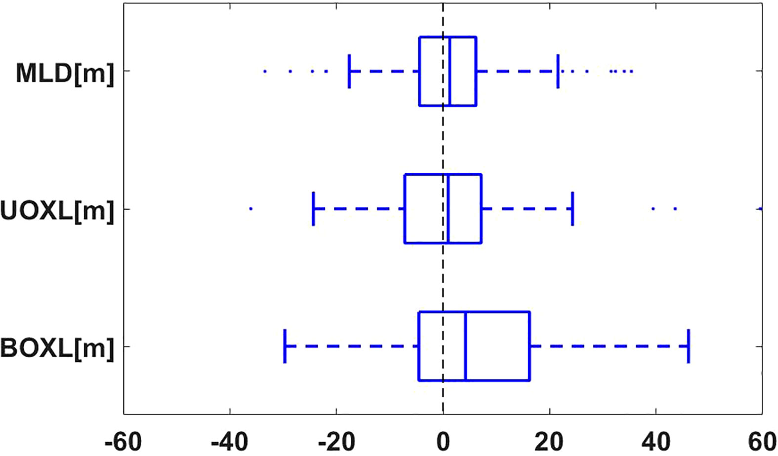
Figure 11 Boxplots of MLD, UOXL and BOXL; blue scatter points represent outliers in the data, the solid blue boxes represent the range of the upper and lower quartiles, and the solid lines inside the boxes are the medians.

4 Summary

In the Arabian Sea, most previous studies on the vertical distribution of dissolved oxygen and the oxycline relied on shipboard observations or few Argo floats. In the last decade, the international BGC-Argo program has collected extensive data profiles of dissolved oxygen with high vertical and temporal resolutions. We used the BGC-Argo data in 2010–2022 to identify the seasonal changes of the oxycline in different regions of the Arabian Sea and determine the principal physical and biological factors that influenced the upper and lower boundaries of the oxycline. In summer and winter, more turbulent mixing supplied more nutrients to the surface layer, resulting in high productivity, and the upper boundary of oxycline was dynamically regulated by MLD. In spring and autumn, the MLD shoaled and the formation of DCM influenced the upper boundary of oxycline; the bottom boundary of oxycline was primarily influenced by the thermocline (pycnocline). Upwelling–downwelling (in the west) and Rossby waves (in the east) regulated the isotherm depth, thus indirectly influencing the bottom boundary of oxycline. These findings highlight the complex interplay between physical and biological factors in shaping the vertical distribution of dissolved oxygen and oxycline dynamics in the Arabian Sea.

Although it was known that the ASHSW subducts and supplies oxygen into the ASOMZ, in this study, we conducted a quantitative analysis of the oxygen introduced into the oxycline and the OMZ via the subduction events. Based on the BGC-Argo data, we found that most of the subduction events primarily occurred in the NE region during the springtime. These events significantly influenced the oxycline and OMZ, by deepening the bottom boundary of oxycline and supplementing oxygen-enriched waters into the oxycline and OMZ. Although subduction has been largely ignored in previous studies, here we found it is an important physical process in reducing hypoxia and keeping denitrification in check in the ASOMZ.

However, it is worth noting that the present distribution of BGC-Argo data is uneven, with a majority of the data concentrated in the NE region. To better quantify the impact of subduction on reducing hypoxia and understand its extent of influence, more BGC-Argo floats need to be deployed in other regions of the Arabian Sea in the future. The regionalization could be also improved with more data, based on the hydrologic characteristics derived from temperature and salinity profiles and the hypoxia extent derived from the oxygen profile. Besides, by accumulating the long-term observation time series, it would be feasible to conduct an in-depth analysis of the interannual variances of the oxycline, particularly focusing on the depth, thickness, and oxygen inventory of the bottom boundary. These indicators would serve as valuable measures for assessing the strength and interannual variabilities of hypoxia in the ASOMZ.

Data availability statement

Publicly available datasets were analyzed in this study. This data can be found here: BGC-Argo original data https://doi.org/10.17882/42182; Monthly sea–surface wind stress and Ekman pumping velocity (EPV) data: https://coastwatch.pfeg.noaa.gov/erddap/files/erdQAstressmday_LonPM180/. Further inquiries can be directed to the corresponding author.

Author contributions

XX and SC designed the concept. YZ was responsible for data processing, analysis and drafting the manuscript. All authors revised the manuscript. All authors contributed to the article and approved the submitted version.

Funding

This work is supported by the National Natural Science Foundation of China (42188102), the Scientific Research Fund of the Second Institute of Oceanography, MNR (QNYC2302), and Southern Marine Science and Engineering Guangdong Laboratory (Zhuhai) (SML2021SP102).

Acknowledgments

The authors are grateful to all the BGC-Argo data providers and the principal investigators of related BGC-Argo float missions and projects (https://doi.org/10.17882/42182). The BGC-Argo data processing and quality control in this study was conducted in the China Argo Real-time Data Center (http://www.argo.org.cn).

Conflict of interest

The authors declare that the research was conducted in the absence of any commercial or financial relationships that could be construed as a potential conflict of interest.

Publisher’s note

All claims expressed in this article are solely those of the authors and do not necessarily represent those of their affiliated organizations, or those of the publisher, the editors and the reviewers. Any product that may be evaluated in this article, or claim that may be made by its manufacturer, is not guaranteed or endorsed by the publisher.

Supplementary material

The Supplementary Material for this article can be found online at: https://www.frontiersin.org/articles/10.3389/fmars.2023.1171614/full#supplementary-material

References

Acharya S. S., Panigrahi M. K. (2016). Eastward Shift and maintenance of Arabian Sea oxygen minimum zone: understanding the paradox. Deep Sea Res. Part I 115, 240–252. doi: 10.1016/j.dsr.2016.07.004

CrossRef Full Text | Google Scholar

Ahmed N. (2021). A study of dynamics of upper high salinity water mass in the Arabian Sea (United Kingdom: Services for Science and Education), 298. doi: 10.14738/eb.40.2020

CrossRef Full Text | Google Scholar

Amol P. (2018). Impact of rossby waves on chlorophyll variability in the southeastern Arabian Sea. Remote Sens. Lett. 9, 1214–1223. doi: 10.1080/2150704x.2018.1504335

CrossRef Full Text | Google Scholar

Bange H. W., Rapsomanikis S., Andreae M. O. (2001). Nitrous oxide cycling in the Arabian Sea. J. Geophys. Res. 106, 1053–1065. doi: 10.1029/1999JC000284

CrossRef Full Text | Google Scholar

Banse K. (1987). Seasonality of phytoplankton chlorophyll in the central and northern Arabian Sea. Deep Sea Res. Part A 34, 713–723. doi: 10.1016/0198-0149(87)90032-X

CrossRef Full Text | Google Scholar

Banse K., Naqvi S. W. A., Narvekar P. V., Postel J. R., Jayakumar D. A. (2014). Oxygen minimum zone of the open Arabian Sea: variability of oxygen and nitrite from daily to decadal timescales. Biogeosciences 11, 2237–2261. doi: 10.5194/bg-11-2237-2014

CrossRef Full Text | Google Scholar

Banse K., Postel J. R. (2009). “Wintertime convection and ventilation of the upper pycnocline in the northernmost Arabian Sea,” in Indian Ocean biogeochemical processes and ecological variability, vol. 185. (Washington DC: American Geophysical Union Geophysical Monograph Series), 87–117. doi: 10.1029/2008GM000704

CrossRef Full Text | Google Scholar

Beal L. M., Ffield A., Gordon A. L. (2000). Spreading of red Sea overflow waters in the Indian ocean. J. Geophys. Res.: Oceans 105, 8549–8564. doi: 10.1029/1999jc900306

CrossRef Full Text | Google Scholar

Boyer T., Conkright M. E., Levitus S. (1999). Seasonal variability of dissolved oxygen, percent oxygen saturation, and apparent oxygen utilization in the Atlantic and pacific oceans. Deep Sea Res. Part I 46, 1593–1613. doi: 10.1016/s0967-0637(99)00021-7

CrossRef Full Text | Google Scholar

Brock J. C., McClain C. R. (1992). Interannual variability in phytoplankton blooms observed in the northwestern Arabian Sea during the southwest monsoon. J. Geophys. Res. 97, 733–750. doi: 10.1029/91jc02225

CrossRef Full Text | Google Scholar

Brock J. C., McClain C. R., Luther M. E., Hay W. W. (1991). The phytoplankton bloom in the northwestern Arabian Sea during the southwest monsoon of 1979. J. Geophys. Res. 96, 20623–20642. doi: 10.1029/91jc01711

CrossRef Full Text | Google Scholar

Cavan E., Trimmer L., Shelley M. F., Sanders R. (2017). Remineralization of particulate organic carbon in an ocean oxygen minimum zone. Nat. Commun. 8, 14847. doi: 10.1038/ncomms14847

PubMed Abstract | CrossRef Full Text | Google Scholar

Chen S., Wells M. L., Huang R., Xue H., Xi J., Chai F. (2021). Episodic subduction patches in the western north pacific identified from BGC-argo float data. Biogeosciences 18, 5539–5554. doi: 10.5194/bg-18-5539-2021

CrossRef Full Text | Google Scholar

Chowdary J. S., Gnanaseelan C., Thompson B., Salvekar P. S. (2005). Water mass properties and transports in the Arabian Sea from argo observations. J. Atmos. Ocean Sci. 10, 235–260. doi: 10.1080/17417530600752825

CrossRef Full Text | Google Scholar

de Boyer Montégut C., Madec G., Fischer A. S., Lazar A., Iudicone D. (2004). Mixed layer depth over the global ocean: an examination of profile data and a profile-based climatology. J. Geophys. Res. 109, C12003. doi: 10.1029/2004jc002378

CrossRef Full Text | Google Scholar

Garcia H. E. (2005). On the variability of dissolved oxygen and apparent oxygen utilization content for the upper world ocean: 1955 to 1998. Geophys. Res. Lett. 32, L09604. doi: 10.1029/2004gl022286

CrossRef Full Text | Google Scholar

Gilly W. F., Beman J. M., Litvin S. Y., Robison B. H. (2013). Oceanographic and biological effects of shoaling of the oxygen minimum zone. Ann. Rev. Mar. Sci. 5, 393–420. doi: 10.1146/annurev-marine-120710-100849

PubMed Abstract | CrossRef Full Text | Google Scholar

Girishkumar M., Ravichandran M., Pant V. (2012). Observed chlorophyll-a bloom in the southern bay of Bengal during winter 2006–2007. Remote Sens. 33, 1264–1275. doi: 10.1080/01431161.2011.563251

CrossRef Full Text | Google Scholar

Gruber N., Lachkar Z., Frenzel H., Marchesiello P., Munnich M., McWilliams J. C., et al. (2011). Eddy-induced reduction of biological production in eastern boundary upwelling systems. Nat. Geosci. 4, 787–792. doi: 10.5194/bg-9-293-2012

CrossRef Full Text | Google Scholar

Gundersen J. S., Gardner W. D., Richardson M. J., Walsh I. D. (1998). Effects of monsoons on the seasonal and spatial distributions of POC and chlorophyll in the Arabian Sea. Deep Sea Res. Part II 45, 2103–2132. doi: 10.1016/s0967-0645(98)00065-4

CrossRef Full Text | Google Scholar

Hu Q., Chen X., Hu X., Bai Y., Zhong Q., Gong F., et al. (2022). Seasonal variability of phytoplankton biomass revealed by satellite and BGC-argo data in the central tropical Indian ocean. J. Geophys. Res. Ocean 127, e2021JC018227. doi: 10.1029/2021jc018227

CrossRef Full Text | Google Scholar

Ito T., Minobe S., Long M. C., Deutsch C. (2017). Upper ocean otrends: 1958–2015. Geophys. Res. Lett. 44, 4214–4223. doi: 10.1002/2017GL073613

CrossRef Full Text | Google Scholar

Jain V., Shankar D., Vinayachandran P. N., Kankonkar A., Chatterjee A., Amol P., et al. (2016). Evidence for the existence of Persian gulf water and red Sea water in the bay of Bengal. Clim. Dynam. 48, 3207–3226. doi: 10.1007/s00382-016-3259-4

CrossRef Full Text | Google Scholar

Johnson K. S., Plant J. N., Riser S. C., Gilbert D. (2015). Air oxygen calibration of oxygen optodes on a profiling float array. J. Atmos. Oceanic Technol. 32, 2160–2172. doi: 10.1175/JTECH-D-15-0101.1

CrossRef Full Text | Google Scholar

Keeling R. E., Kortzinger A., Gruber N. (2010). Ocean deoxygenation in a warming world. Ann. Rev. Mar. Sci. 2, 199–229. doi: 10.1146/annurev.marine.010908.163855

PubMed Abstract | CrossRef Full Text | Google Scholar

Kumar T. P., Kumar S. S., Maheswaran P. A. (2019). Intra annual variability of the Arabian Sea high salinity water mass in the south Eastern Arabian Sea during 2016-17. Def. Sci. J. 69, 149–155. doi: 10.14429/dsj.69.14217

CrossRef Full Text | Google Scholar

Kumar S. P., Prasad T. G. (1999). Formation and spreading of Arabian Sea high-salinity water mass. J. Geophys. Res. Ocean 104, 1455–1464. doi: 10.1029/1998jc900022

CrossRef Full Text | Google Scholar

Kumar S. P., Ramaiah N., Gauns M., Sarma V. V. S. S., Muraleedharan P. M., Raghukumar S., et al. (2001). Physical forcing of biological productivity in the northern Arabian Sea during the northeast monsoon. Deep Sea Res. Part II 48, 1115–1126. doi: 10.1016/j.dsr2.2005.06.002

CrossRef Full Text | Google Scholar

Kumar S. P., Narvekar J. (2005). Variability of the mixed layer in the central Arabian Sea and its implication on nutrients and primary productivity. Deep Sea Res. Part II 14-15, 1848–1861. doi: 10.1016/j.dsr2.2005.06.002

CrossRef Full Text | Google Scholar

Lachkar Z., Lévy M., Smith S. (2018). Intensification and deepening of the Arabian Sea oxygen minimum zone in response to increase in Indian monsoon wind intensity. Biogeosciences 15, 159–186. doi: 10.5194/bg-15-159-2018

CrossRef Full Text | Google Scholar

Lachkar Z., Lévy M., Smith K. S. (2019). Strong intensification of the Arabian Sea oxygen minimum zone in response to Arabian gulf warming. Geophys. Res. Lett. 46, 5420–5429. doi: 10.1029/2018gl081631

CrossRef Full Text | Google Scholar

Laffoley D., Baxter J. M. (2019). Ocean deoxygenation: everyone’s problem-causes, impacts, consequences and solutions (Switzerland: IUCN Gland), 580. doi: 10.2305/IUCN.CH.2019.13

CrossRef Full Text | Google Scholar

Laxenaire R., Speich S., Blanke B., Chaigneau A., Pegliasco C., Stegner A. (2018). Anticyclonic eddies connecting the Western boundaries of Indian and Atlantic oceans. J. Geophys. Res. Oceans 123, 7651–7677. doi: 10.1029/2018JC01427

CrossRef Full Text | Google Scholar

Llort J., Langlais C., Matear R., Moreau S., Lenton A., Strutton P. G. (2018). Evaluating southern ocean carbon eddy-pump from biogeochemical-argo floats. J. Geophys. Res. Oceans 123, 971–984. doi: 10.1002/2017JC012861

CrossRef Full Text | Google Scholar

Lotliker A. A., Baliarsingh S. K., Samanta A., Varaprasad V. (2020). Growth and decay of high-biomass algal bloom in the northern Arabian Sea. J. Indian Soc Remote Sens. 48, 465–471. doi: 10.1007/s12524-019-01094-3

CrossRef Full Text | Google Scholar

Madhupratap M., Kumar S. P., Bhattathiri P., Kumar M. D., Raghukumar S., Nair K., et al. (1996). Mechanism of the biological response to winter cooling in the northeastern Arabian Sea. Nat 384, 549–552. doi: 10.1038/384549a0

CrossRef Full Text | Google Scholar

Matear R. J., Hirst A. C. (2003). Long-term changes in dissolved oxygen concentrations in the ocean caused by protracted global warming. global biogeochem. Cycles 17, 1125. doi: 10.1029/2002gb001997

CrossRef Full Text | Google Scholar

Mathew T., Prakash S., Shenoy L., Chatterjee A., Udaya Bhaskar T. V. S., Wojtasiewicz B. (2021). Observed variability of monsoon blooms in the north-central Arabian Sea and its implication on oxygen concentration: a bio-argo study. Deep Sea Res. Part II 184-185, 104935. doi: 10.1016/j.dsr2.2021.104935

CrossRef Full Text | Google Scholar

McCreary J., Murtugudde R., Vialard J., Vinayachandran P. N., Wiggert J. D., Hood R. R., et al. (2009). Biophysical processes in the Indian ocean. Indian Ocean Biogeochemical Processes Ecol. Variability 185, 9–32. doi: 10.1029/2008GM000768

CrossRef Full Text | Google Scholar

McCreary J. P., Zuojun Y., Hood R. R., Vinaychandran P. N., Furue R., Ishida A., et al. (2013). Dynamics of the Indian-ocean oxygen minimum zones. Progr. Oceanogr. 112-113, 15–37. doi: 10.1016/j.pocean.2013.03.002

CrossRef Full Text | Google Scholar

Morrison J. M., Codispoti L. A., Gaurin S., Jones B., Manghnani V., Zheng Z. (1998). Seasonal variation of hydrographic and nutrient fields during the US JGOFS Arabian Sea process study. Deep Sea Res. Part II 45, 2053–2101. doi: 10.1016/s0967-0645(98)00063-0

CrossRef Full Text | Google Scholar

Morrison J. M., Codispoti L. A., Smith S. L., Wishner K., Flagg C., Gardner W. D., et al. (1999). The oxygen minimum zone in the Arabian Sea during 1995. Deep Sea Res. Part II 46, 1903–1931. doi: 10.1016/s0967-0645(99)00048-x

CrossRef Full Text | Google Scholar

Naqvi S. W. A. (1987). Some aspects of the oxygen-deficient conditions and denitrification in the Arabian Sea. J. Mar. Res. 45, 1049–1072. doi: 10.1357/002224087788327118

CrossRef Full Text | Google Scholar

Naqvi S. W. A. (1991). Geographical extent of denitrification in the Arabian Sea in relation to some physical processes. Oceanol. Acta 14, 281–290.

Google Scholar

Paterson H. L., Feng M., Waite A. M., Gomis D., Beckley L. E., Holliday D., et al. (2008). Physical and chemical signatures of a developing anticyclonic eddy in the leeuwin current, eastern Indian ocean. J. Geophys. Res. Lett. 113, C07049. doi: 10.1029/2007JC004707

CrossRef Full Text | Google Scholar

Piontkovski S. A., Al-Oufi H. S. (2015). The omani shelf hypoxia and the warming Arabian Sea. Int. J. Environ. Stud. 72, 256–264. doi: 10.1080/00207233.2015.1012361

CrossRef Full Text | Google Scholar

Piontkovski S. A., Queste B. Y. (2016). Decadal changes of the Western Arabian Sea ecosystem. Int. Aquat. Res. 8, 49–64. doi: 10.1007/s40071-016-0124-3

CrossRef Full Text | Google Scholar

Prakash S., Nair T. M. B., Bhaskar T. V. S. U., Prakash P., Gilbert D. (2012). Oxycline variability in the central Arabian Sea: an argo-oxygen study. J. Sea Res. 71, 1–8. doi: 10.1016/j.seares.2012.03.003

CrossRef Full Text | Google Scholar

Prakash S., Prakash P., Ravichandran M. (2013). Can oxycline depth be estimated using sea level anomaly (SLA) in the northern Indian ocean? Remote Sens. Lett. 4, 1097–1106. doi: 10.1080/2150704x.2013.842284

CrossRef Full Text | Google Scholar

Prasad T. G. (2002). A numerical study of the seasonal variability of Arabian Sea high-salinity water. J. Geophys. Res. 107, 3197. doi: 10.1029/2001jc001139

CrossRef Full Text | Google Scholar

Prasad T. G., Ikeda M., Kumar S. P. (2001). Seasonal spreading of the Persian gulf water mass in the Arabian Sea. J. Geophys. Res. Ocean 106, 17059–17071. doi: 10.1029/2000jc000480

CrossRef Full Text | Google Scholar

Prasanth R., Vijith V., Thushara V., George J. V., Vinayachandran P. N. (2021). Processes governing the seasonality of vertical chlorophyll-a distribution in the central Arabian Sea: bio-argo observations and ecosystem model simulation. Deep Sea Res. Part II 183, 104926. doi: 10.1016/j.dsr2.2021.104926

CrossRef Full Text | Google Scholar

Queste B. Y., Vic C., Heywood K. J., Piontkovski. S. A. (2018). Physical controls on oxygen distribution and denitrification potential in the north West Arabian Sea. Geophys. Res. Lett. 45, 4143–4152. doi: 10.1029/2017gl076666

CrossRef Full Text | Google Scholar

Ravichandran M., Girishkumar M. S., Riser S. (2012). Observed variability of chlorophyll-a using argo profiling floats in the southeastern Arabian Sea. Deep Sea Res. Part I 65, 15–25. doi: 10.1016/j.dsr.2012.03.003

CrossRef Full Text | Google Scholar

Resplandy L., Lévy M., Bopp L., Echevin V., Pous S., Sarma V. V. S. S., et al. (2012). Controlling factors of the oxygen balance in the Arabian sea’s OMZ. Biogeosciences 9, 5095–5109. doi: 10.5194/bg-9-5095-2012

CrossRef Full Text | Google Scholar

Rixen T., Cowie G., Gaye B., Goes J., Do Rosário Gomes H., Hood R. R., et al. (2020). Reviews and syntheses: present, past, and future of the oxygen minimum zone in the northern Indian ocean. Biogeosciences 17, 6051–6080. doi: 10.5194/bg-17-6051-2020

CrossRef Full Text | Google Scholar

Rixen T., Ittekkot V. (2005). Nitrogen deficits in the Arabian Sea, implications from a three component mixing analysis. Deep Sea Res. Part II 52, 1879–1891. doi: 10.1016/j.dsr2.2005.06.007

CrossRef Full Text | Google Scholar

Sarma V. V. S. S., Bhaskar T. V. S. U., Kumar J. P., Chakraborty K. (2020). Potential mechanisms responsible for occurrence of core oxygen minimum zone in the north-eastern Arabian Sea. Deep Sea Res. Part I 165, 103393. doi: 10.1016/j.dsr.2020.103393

CrossRef Full Text | Google Scholar

Scheffzek K., Lautwein A., Kabsch W., Ahmadian M. R., Wittinghofer A. (1996). Crystal structure of the GTPase-activating domain of human p120 GAP and implications for the interaction with ras. Nat 384, 591–596. doi: 10.1038/384591a0

CrossRef Full Text | Google Scholar

Schmidt H., Czeschel R., Visbeck M. (2020). Seasonal variability of the Arabian Sea intermediate circulation and its impact on seasonal changes of the upper oxygen minimum zone. Ocean Sci. 16, 1459–1474. doi: 10.5194/os-16-1459-2020

CrossRef Full Text | Google Scholar

Schmidt H., Getzlaff J., Löptien U., Oschlies A. (2021). Causes of uncertainties in the representation of the Arabian Sea oxygen minimum zone in CMIP5 models. Ocean Sci. 17, 1303–1320. doi: 10.5194/os-17-1303-2021

CrossRef Full Text | Google Scholar

Schmidtko S., Stramma L., Visbeck M. (2017). Decline in global oceanic oxygen content during the past five decades. Nat 542, 335–339. doi: 10.1038/nature21399

CrossRef Full Text | Google Scholar

Schott F. A., McCreary J. P. (2001). The monsoon circulation of the Indian ocean. Progr. Oceanogr. 51, 1–123. doi: 10.1016/S0079-6611(01)00083-0

CrossRef Full Text | Google Scholar

Shenoy D. M., Suresh I., Uskaikar H., Kurian S., Vidya P. J., Shirodkar G., et al. (2020). Variability of dissolved oxygen in the Arabian Sea oxygen minimum zone and its driving mechanisms. Mar. Syst. 204, 103310. doi: 10.1016/j.jmarsys.2020.103310

CrossRef Full Text | Google Scholar

Shetye S. R., Gouveia A. D., Shenoi S. S. C. (1994). Circulation and water masses of the Arabian Sea. J. Earth Syst. Sci. 103, 107–123. doi: 10.1007/bf02839532

CrossRef Full Text | Google Scholar

Singh S., Valsala V., Prajeesh A. G., Balasubramanian S. (2019). On the variability of Arabian Sea mixing and its energetics. J. Geophys. Res. Ocean 124, 7817–7836. doi: 10.1029/2019jc015334

CrossRef Full Text | Google Scholar

Sreenivas P., Patnaik K. V. K. R. K., Prasad K. V. S. R. (2008). Monthly variability of mixed layer over Arabian Sea using ARGO data. Mar. Geod. 31, 17–38. doi: 10.1080/01490410701812311

CrossRef Full Text | Google Scholar

Stramma L., Johnson G. C., Sprintall J., Mohrholz V. (2008). Expanding oxygen-minimum zones in the tropical oceans. Sci 320, 655–658. doi: 10.1126/science.1153847

CrossRef Full Text | Google Scholar

Thadathil P., Thoppil P., Rao R. R., Muraleedharan P. M., Somayajulu Y. K., Gopalakrishna V. V., et al. (2008). Seasonal variability of the observed barrier layer in the Arabian Sea. J. Phys. Oceanogr. 38, 624–638. doi: 10.1175/2007JPO3798.1

CrossRef Full Text | Google Scholar

Thierry V., Bittig H., the Argo-BGC team. (2021). Argo quality control manual for dissolved oxygen concentration v2.1. doi: 10.13155/46542

CrossRef Full Text | Google Scholar

Trott C. B., Subrahmanyam B., Chaigneau A., Stork. H. L. (2019). Eddy-induced temperature and salinity variability in the Arabian Sea. Geophys. Res. Lett. 46, 2734–2742. doi: 10.1029/2018GL081605

CrossRef Full Text | Google Scholar

Ulloa O., Canfield D. E., DeLong E. F., Letelier R. M., Stewart F. J. (2012). Microbial oceanography of anoxic oxygen minimum zones. Proc. Natl. Acad. Sci. U. S. A. 109, 15996–16003. doi: 10.1073/pnas.1205009109

CrossRef Full Text | Google Scholar

Williams R. G., Follows M. J. (2003). Physical transport of nutrients and the maintenance of biological production. Ocean Biogeochemistry. (Berlin Heidelberg: Springer) pp. 19–51. doi: 10.1007/978-3-642-55844-3_3

CrossRef Full Text | Google Scholar

Xing X., Claustre H., Blain S., D’Ortenzio F., Antoine D., Ras J., et al. (2012). Quenching correction for in vivo chlorophyll fluorescence acquired by autonomous platforms: a case study with instrumented elephant seals in the kerguelen region (Southern ocean). Limnol. Oceanogr. Meth. 10, 483–495. doi: 10.4319/lom.2012.10.48

CrossRef Full Text | Google Scholar