 P. Munk
 B. Buongiorno Nardelli
 P. Mariani
 J. Bendtsen
- 1National Institute of Aquatic Resources, Technical University of Denmark, Kongens Lyngby, Denmark
- 2Institute of Marine Sciences, National Research Council (ISMAR-CNR), Naples, Italy
- 3ClimateLab, Copenhagen, Denmark
The larvae of the European eel travel an extensive distance of approximately 5,000 km from the spawning area in the Sargasso Sea to the European coasts. We here study the larval drift with focus on the effects of mesoscale processes, analyzing data from a targeted survey and modeling possible drift trajectories. The survey covered the initial distribution of larvae in the Subtropical Convergence Zone (STCZ), which is characterized by complex patterns of oceanic fronts and mesoscale eddies. During March–April 2014, sampling was carried out along north–south transects. Hydrography was described using vertical CTD casts and UCTD profiles, and larval distributions assessed from hauls of a large ring net. Patterns in water mass distribution and particle dispersion dynamics were analyzed by reconstruction and diagnosis of mesoscale dynamics, combining satellite observations and Argo profiles. Lagrangian drift trajectories of eel larvae were subsequently simulated starting from a data-driven high-resolution 3D reconstruction of the modeled flow. We found the area of larval distribution delimited by frontal zones, defined by the combined effects of marked longitudinal salinity gradients and large-scale zonal temperature variations. Modeled patterns of eel larvae dispersion were predominantly influenced by the current shear and eddy strain, and while the direction was mainly westward, a significant dispersal was also observed in northeastward directions. Such almost isotropic transport of European eels is supported by historical data on larval size distribution, and results challenge common interpretations of eel larval drift, which propose an initial westward advection of the entire population to the Gulf Stream along the offshore edge of the Antilles current.
1 Introduction
Freshwater eels of the genus Anguilla migrate to offshore areas for their spawning. All species appear to spawn in subtropical marine areas, but distances of migration differ substantially among the species (Aoyama, 2009). Species from temperate foraging areas generally have longer migration routes than those from tropical areas (Kuroki et al., 2014), the route of the European eel being the absolute longest, of approximately 5,000 km (Schmidt, 1922). Irrespective of the differences in their distance from coast, the spawning areas of freshwater eels have a number of common characteristics. These areas are found where subtropical water meets colder water masses and they are dominated by prominent eddies and fronts. The fronts are characterized by strong gradients in either temperature or salinity (Kleckner and McCleave, 1988; Kimura et al., 1994). An additional characteristic of the spawning sites, potentially directing eel during migration, is the presence of subducted highly saline water masses (Schabetsberger et al., 2016). These water masses appear as cores of elevated salinities (~35.0 to 36.8) at depths of approximately 150 m and are observed at the major spawning areas of freshwater eels across the world (Schabetsberger et al., 2016). In these areas, weak westward currents (~0 to 0.1 m s−1) prevail, but eastward surface countercurrents can also be observed (Cushman-Roisin, 1984).
In the Atlantic, the spawning areas of European and American freshwater eels (Anguilla anguilla and A. rostrata, respectively) appear linked to the so-called Subtropical Convergence Zone (STCZ), a transition zone in the southern Sargasso Sea where Northern Atlantic water masses meet subtropical water masses (Kleckner and McCleave, 1988; Munk et al., 2010). The spawning areas of the species were identified from the distributions of early larval stages, while no spawning adults and no eggs have yet been observed. The first descriptions of newly hatched larvae of the two Atlantic eel species, and their areas of distribution, were based on extensive cruises in the years 1914–1922 (Schmidt, 1922). There is some distributional overlap between larvae of the two species, but their centers of distribution are significantly displaced, with the European eel larvae more easterly distributed. The early cruises in 1914–1922 were focused on an apparent key area of European eel larvae distribution within 23°N–26°N and 71°W–60°W, and this area has been in focus during the subsequent series of cruises investigating spawning sites of Atlantic eels. However, small European eel larvae can be found farther to the east, as far as 50°W (Schmidt, 1922; Schoth and Tesch, 1982; Miller et al., 2019), and sampling of older larvae east of 50°W suggests that at least some of the European eel larvae directly drift north- and eastwards from the spawning area (Kracht, 1982).
A number of oceanographic modeling studies propose an initial drift of European eel larvae from the spawning site towards the west, whereafter these larvae are entrained in the Antilles and Florida currents and subsequently advected towards Europe by the Gulf Stream and the North Atlantic drift (Kettle and Haines, 2006; Bonhommeau et al., 2009; Melià et al., 2013; Baltazar-Soares et al., 2014; Pacariz et al., 2014). The proposed dominance of an initial westward drift of the larvae contradicts, however, the abovementioned observations of the easterly distributions of European eel larvae and also the observations of increasing mean sizes in a north-eastward direction from the central site of spawning (Schmidt, 1922; Kracht, 1982; Miller et al., 2015). Thus, alternative northeastward routes of European eel larval dispersal and drift have been proposed (McCleave, 1993; Munk et al., 2010; Miller et al., 2015). A more recent modeling exercise indicated strong retention in the area of the Sargasso Sea while most modeled European eel larvae remained dispersed in the southern Sargasso Sea during their first months of life, and only a minor fraction left the area, entrained into the initial flow of the Gulf Stream (Westerberg et al., 2017). Thus, the interpretations of the drift patterns of European eel larvae remain inconclusive and there is a further need for process-oriented studies of larval drift.
The STCZ—where the early eel larvae are predominantly distributed—has a complex hydrography, which is influenced by the strong meanders and eddies modulating the North Atlantic subtropical gyre circulation, and simulations of larval dispersion and drift in this area would need to correctly resolve these mesoscale features. Many oceanographic models studying eel larval drift are based on general circulation models at different resolutions, including eddy resolving models (as referred to above). Here, we follow a different approach, where observation-based reconstructions of the ocean state are used to estimate the horizontal and vertical components of the ocean circulation, solving directly for mesoscale structures and dynamics (e.g., Mason et al., 2017; Barceló-Llull et al., 2018; Buongiorno Nardelli et al., 2018). Our methodology combines satellite and in situ observations and semi-geostrophic diagnostic equations. It uses multivariate statistical interpolation and 3D data extrapolation methods to achieve the spatial and temporal resolutions needed to describe the mesoscale dynamics (1/10° resolution). It specifically describes 3D vertical velocities driven by the internal dynamics, thus going beyond the purely 2D geostrophic characterization provided by standard processing (e.g., Mulet et al., 2012).
These data-driven reconstructions of ocean currents are combined with Lagrangian dispersion modeling to analyze the potential importance of mesoscale features, current patterns, and larvae vertical behavior, investigating the initial phase (first 6 months) of eel larval dispersal and drift in and from the Sargasso Sea. Modeling and analyses were based on in situ observations of eel larvae distributions and corresponding hydrography, as well as on satellite and drifting buoy information obtained during a dedicated oceanographic cruise in 2014. We specifically investigate whether larval transport could lead to entrainment of larvae into drift routes to the north and east of the spawning area, and interpret findings in relation to historical observations of larval size groups distributed across the North Atlantic. Our approach aims at challenging the prevailing interpretation of drift routes of European eel larvae, which suggests that the single most important transport mechanism of European eel larvae is advection towards west, and subsequent entrainment in the Florida Current and in the western part of the Gulf Stream (e.g., Bonhommeau et al., 2009; Blanke et al., 2012).
2 Data and methods
2.1 Survey information, CTD casts
In situ information were gained during a cruise by r/v Dana (National Institute of Aquatic Sciences, Technical University of Denmark) carried out 15 March to 23 April 2014. Stations of sampling and measurement during the cruise were positioned along longitudinal transects basically perpendicular to the hydrographic fronts in the area. Total area of sampling extended from 68°30′W to 37°40′W (Figure 1A), but stations in the area east of 50°00′W (where no larvae were caught) are not included in the present study. Included transects were aligned 3°C longitude from each other, and station distances along transects ranged from 10 to 20 nautical miles (Figure 1B). At each station, temperature and salinity were profiled vertically in 0.5-m intervals to 400 m using a Seabird 9/11 CTD equipped with a 12 Niskin bottle rosette sampler. Further CTD measurements were carried out along transect 3 using an underway-CTD (UCTD, OceanScience). The UCTD is designed to measure profiles from a moving ship and it was applied in free-falling mode (rate of descent: ~4 m s−1) down to 400 m with a ship speed of ~10 knots.
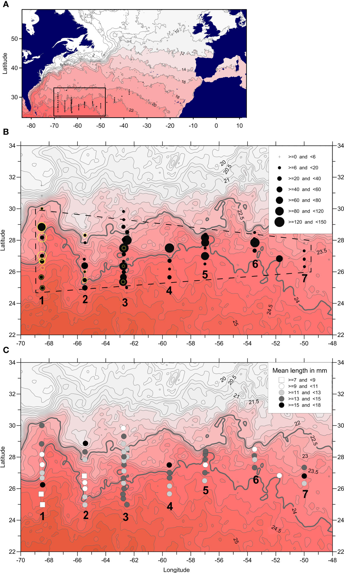
Figure 1 Sampling during the cruise. (A) Position of stations, rectangle encloses area shown in (B, C). Contouring illustrates the change in SST on the 2th April 2014 with isotherms at 2°C intervals. (B) Abundances of anguillid larvae at the westernmost seven transects of sampling, these labelled 1-7. Sizes of black circles illustrate relative abundances of A anguilla, sizes of light rings denote A rostrata. Background as for (A) with isotherms at 0.25°C intervals, and the 22.5°C and 24.0°C isotherms indicated by heavier lines. Hatched lines denote area of observed larval distribution. (C) Mean sizes of A anguilla illustrated by different symbols, intervals of size as in legend.
2.2 Survey information, sampling of European and American eel larvae
Eel larvae were sampled at each station by a ring net of diameter 3.5 m equipped with a 25-m-long net of 560-µm mesh. The gear was lowered to 250 m in an oblique haul, at a ship speed of 2.5 knots and a wire pay-out and retrieval of 25 and 15 m min−1, respectively. The distance towed was measured by the ships’ positioning system. Sampled larvae were stored in alcohol, and later eel larvae were identified by genetic analysis as described by Jacobsen et al. (2017). Using information on catch, area of gear opening, distance towed, and the depth of haul, the abundances of A. anguilla and A. rostrata were expressed by number per unit surface area. Lengths of the majority of larvae were estimated shortly after catch and when unpreserved. Some of the larvae caught were however sorted from the alcohol-preserved samples after the cruise, and their lengths were converted by the formula: unpreserved L (mm) = preserved L (mm) * 1.16 − 4.36; this was estimated from a group of larvae (range 7–19 mm) measured individually before and after preservation.
2.3 Historical information on European eel larvae distributions and lengths
Historical data on catches and size of European eel, sampled during the period 1914–2007, were downloaded from a database at the International Council for Exploration of the Seas: http://eggsandlarvae.ices.dk/Download.aspx. For all stations, irrespective of time of year, estimates of abundances per unit area and the average total length were estimated and all station observations were contoured using the “inverse distance” procedure of interpolation in the 3D mapping and analysis software SURFER ©.
2.4 Estimation of geostrophic velocities
Geostrophic velocities were estimated from CTD profiles along the survey transects and based on dynamic height anomalies calculated from TEOS10 (IOC et al., 2010) using a reference pressure of 400 dbar (i.e., the deepest measurements in the profiles). Comparisons were also made between the corresponding steric height anomalies along the transects and daily merged absolute dynamic topography obtained from AVISO (1/4° resolution; SSALT/Duacs L4 product, www.aviso.altimetry.fr) averaged over the period for each transect passage.
2.5 Semi-geostrophic diagnostics
In order to describe the evolution of the mesoscale field before, during, and after the survey, a 3D reconstruction of the semi-geostrophic dynamics was carried out. Similar to previous reconstructions of the Agulhas region (Buongiorno Nardelli, 2013) and Antarctic Circumpolar Current (Buongiorno Nardelli et al., 2018), this analysis was based on a multivariate combination of satellite measurements and in situ Argo/CTD profiles and the application of diagnostic tools at higher-order approximation with respect to standard geostrophic methods. The technique consists of three separate steps (which will be described further in subsections below): (1) the collection/development of high-resolution (1/10°) interpolated Sea Surface Temperature (SST), Absolute Dynamic Topography (ADT), and Sea Surface Salinity (SSS) data; (2) the vertical projection of the surface fields; and (3) the application of a diagnostic tool to retrieve the ageostrophic components of the flow from synthetic 3D temperature (T) and salinity (S) fields. The resulting 3D flow field data were successively used to perform numerical simulations of larval dispersion using a particle-tracking algorithm that accounts for the vertical behavior of the larvae. This dataset and part of the processing chains also served as demonstrators/prototypes for the design of the European Space Agency World Ocean Circulation (ESA-WOC) project (https://www.worldoceancirculation.org), where an extended time series has been produced to be used within specific tasks dedicated to sustainable fisheries (i.e., ESA-WOC Theme 2 activities).
2.6 High-resolution surface data
The SST used is the 1/10° resolution, daily Odyssea L4 developed by Ifremer in the framework of the MERSEA project and maintained as part of the European Copernicus Marine Service (https://doi.org/10.48670/mds-00321). Odyssea L4 is based on the combination and interpolation of microwave and infrared measurements (Piollè and Autret, 2023, https://catalogue.marine.copernicus.eu/documents/QUID/CMEMS-SST-QUID-010-043.pdf). The ADT data used here are the delayed-time optimally interpolated daily maps (Pujol et al., 2016) obtained from Jason-1, Jason-2, and Envisat altimeter data that are distributed through the framework of Copernicus Marine Service (https://doi.org/10.48670/moi-00148), through a 2D spline to 1/10° resolution. The SSS data have been obtained by applying the multidimensional optimal interpolation algorithm adopted within Copernicus Marine Service to retrieve the global SSS and Sea Surface Density (SSD) optimally interpolated 1993–2017 dataset (Droghei et al., 2018).
2.7 Projection of surface data to the subsurface
The technique used here to derive the 3D fields of temperature and salinity is the multivariate Empirical Orthogonal Function Reconstruction (mEOF-R) (Buongiorno Nardelli et al., 2012). This method first computes the EOFs describing the variability of the state vector built from (normalized) temperature, salinity, and steric height profiles, and then uses them to project the corresponding surface fields (SST, SSS, and ADT) to the subsurface. For each grid point, mEOF-R reconstructs the vertical profile combining up to three mEOFs (Buongiorno Nardelli et al., 2017).
The T/S vertical profiles used as input to the mEOF-r are the quality-controlled ARGO and CTD profiles pre-processed by the Coriolis In Situ Analysis System (ISAS) (Gaillard et al., 2009). These data are presently disseminated through Copernicus Marine Service as COriolis dataset for Re-Analysis (CORA, Cabanes et al., 2013). 3D T and S fields were thus obtained through mEOF-r on the Odyssea L4 horizontal grid with a vertical resolution of 10 m down to 1,000 m depth. The domain considered covers the longitudinal/latitudinal range 80°W–20°W and 20°N–45°N. A fully independent validation of the 3D T/S fields was obtained by comparing the synthetic profiles with co-located in situ profiles collected during the cruise. In the present case, the reconstruction based on two modes performed better than the three (and single)-mode configuration. Indeed, more than 99% of the variance was generally explained by the first two modes. The temperature and salinity RMSE are, respectively, approximately 0.5°C and 0.15 psu at the surface, and do not exceed 1.0°C and 0.2 psu along the water column. The 3D geostrophic velocities were then estimated from T and S fields, referenced to the sea surface.
2.8 Omega equation
From the synthetic 3D fields described above, it is possible to retrieve the vertical velocity field by applying the Semi-Geostrophic Omega equation with Dirichlet conditions imposed at the surface and at topographical boundaries (i.e., zero vertical flow), and Neumann conditions at the bottom and lateral boundaries (namely, zero horizontal gradients of the vertical velocities) (Buongiorno Nardelli et al., 2018). Here, the equation was solved numerically considering only the adiabatic forcings, i.e., neglecting the impact of upper layer mixing driven by air–sea interactions on the semi-geostrophic dynamics. Indeed, even if the mixing effect of wind-driven momentum exchange and heat fluxes at the surface has been included in recent lower-resolution (1/4°× 1/4°) reconstructions (Buongiorno Nardelli et al., 2018; Buongiorno Nardelli, 2020b), its impact within the layer where eel larvae live (50–150 m) was assessed to be much lower than the impact of not being able to properly resolve horizontal gradients and related adiabatic dynamics at 1/4° resolution (Buongiorno Nardelli et al., 2012). An extension of present dynamical reconstruction including diabatic forcing terms has been completed very recently in the framework of the ESA-WOC project but is not included here.
2.9 Particle tracking
The particle-tracking algorithm simulates the trajectory of eel larvae by integrating over time the synthetic velocity fields described above and a prescribed diel vertical migration of the larvae. Based on larval age distribution, average spawning time for the sampled larvae has been estimated to 28 February 2014 (Ayala and Munk, 2018). Consistent with observations, 15 February 2014 has been used as initial conditions in the modeling of larval distribution.
Turbulent diffusion is included using the Smagorinsky method (Smagorinsky, 1963) with the Smagorinsky’s constant C = 0.1 and a background diffusivity of 50 m2 day−1. This very small background diffusivity is used only to guarantee non-zero solutions when interpolating ocean currents in the turbulent closure model. Different values of these parameters (i.e., tested range 10 m2 day−1 to 100 m2 day−1 and C = 0.1–0.2) have no significant effects on the results (see below). The dynamic equation is solved with a fourth-order Runge-Kutta method and a time step of 4 h, in the period between March and November 2014. We tested whether the second-order integration schemes and the shorter integration time steps had no significant effects on the results (less than 1% change in the dispersion values from the spawning area, see below).
Particles were uniformly released in a vertical layer between 50 m and 150 m and over the area of European larvae distribution as observed during the cruise. The region of spawning is defined between 24°CN–30°CN and 50°CW–70°CW (Figure 1). The trajectories of 1 million particles were simulated with the model, and particles’ positions and concentrations were calculated at each time step. The number of particles is sufficient to cover all the numerical grid boxes in the spawning areas. Indeed, we tested the model using half the number of particles (still sufficient to have all boxes covered) obtaining similar results.
As suggested by observations during the present cruise (Munk et al., 2018), numerical larvae were assumed to actively migrate towards deeper layers (150 m) during daylight while migrating towards the surface (50 m) at night. These migrations were assumed to occur at a constant speed (relative to the background vertical flow) of 5 mm s−1, a value that reproduces observed migration patterns. Different diel vertical migration (DVM) models have been tested to assess the impacts on the results. Specifically, different depths during daylight have been used (i.e., 60 m, 75 m, and 100 m) as well as no DVM forcing particles to keep the same depth during simulations (i.e., 50 m and 150 m, respectively). Vertical movements were modeled using a solar radiation algorithm with a solar constant of 1,370 W m−2 and accounting for Earth’s orbit ellipticity and absorption through the atmosphere (SEA-MAT, 2022). This provides a solar radiance at the surface of the ocean and a threshold radiance value of 10-10 W m−2 was used to distinguish between night and day in the model, prompting a change in the direction of vertical migrations.
3 Results
3.1 General hydrographic conditions in March 2014
The STCZ, i.e., the area between the westerlies and the trade winds, is characterized by a dynamic mesoscale eddy field (Ullman et al., 2007), and their influence was also visible from the SST during the 2014 cruise (Figure 1). Relatively warm (>24°C) surface water masses characterized the southern part of the transects (except the three easternmost that were entirely located north of the 24°C isotherm) and colder water masses (~22°C) were located north of ~29°CN. The northern frontal zones were seen in the western transects as outcropping isotherms in the upper 100–150 m (Figures 2A–C). Subtropical Underwater (STUW) is present in subtropical gyres and could also be identified by its high salinity (S > 36.73; O’Connor et al., 2005) at all the transects. It was located below 100 m at transects 1 and 2 whereas shallower high surface salinity locations at transect 3 indicated that the northern part was near its formation area (Figures 2D–F). Temperature and salinity gradually decreased below ~200 m towards the Subtropical Mode Water located at ~400 m depth (STMW, also denoted Eighteen Degree Water; Talley and Raymer, 1982).
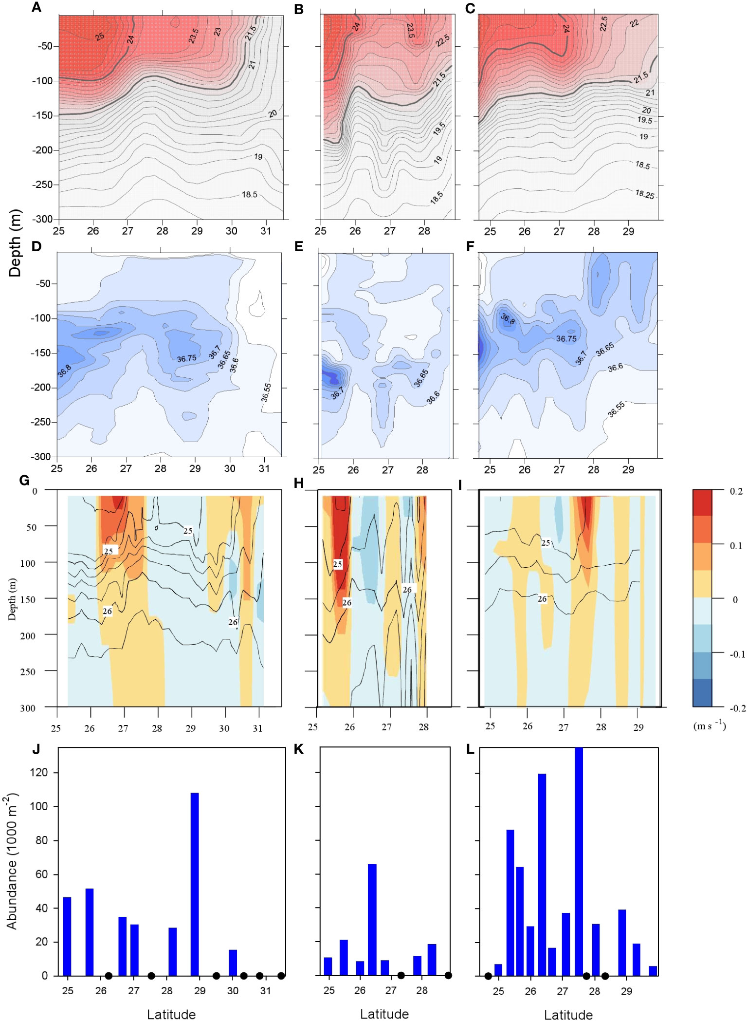
Figure 2 Vertical profiles of hydrographic characteristics and larval distribution along transects 1-3. (A–C) Transects 1-3, Profiling of temperature (°C), isotherms every 0.25°C, the 21.5°C and 24.0°C isotherms shown by heavier lines. (D–F) Transects 1-3. Profiling of salinity, halolines every 0.05 ppm. (G–I) Transects 1-3, water density (sigma-t) isopycnals every 0.5 kg m-3, shading illustrates geostrophic velocity, levels indicated by inserted bar. (J–L) Transects 1-3, bars illustrate A.anguilla abundance (1000 m-2).
An eastward current component of 0.1–0.2 m s−1 characterized the frontal zones associated with the large meandering and eddying mesoscale field and the maximum horizontal current shear was localized near the outcropping of the 24.75 kg m−3 isopycnal along transects 1 and 2, and the 25.0 kg m−3 along transect 3 (Figures 2G–I). The strongest eastward current along transect 1 was observed in a frontal zone centered at 26.9°CN where the current was above 0.15 m s−1 in the upper 30 m, remained above 0.1 m s−1 down to 60 m depth, and then gradually decreased to 0.02 m s−1 at 200 m depth. Similarly strong currents were observed along transect 2 in a frontal zone centered approximately 25.7°CN where the eastward current was above 0.3 m s−1 down to 60 m depth and remained above 0.15 m s−1 down to 150 m depth. A narrow frontal zone with currents above 0.2 m s−1 in the upper 30 m was located at 27.6°CN along transect 3. The eastward baroclinic currents in the frontal zones were mainly confined to the upper 100–200 m and located above the 26.0 kg m−3 isopycnal. A general agreement was seen between satellite-derived absolute dynamic topography and steric height calculated from CTD stations along the transect (not shown), and this supported the estimated geostrophic velocities.
During the period of the survey, the mesoscale field in the Sargasso Sea was dominated by the presence of a large meander, well visible at the surface in the western part of the domain (Figure 3). This meander was characterized by a general eastward flow (e.g., seen as an eastward current at transect 1 at 26.9°CN, Figure 2). The frontal meander was created by the combined effect of a large-scale zonal sea surface temperature variation (Figure 3A) and a marked, but relatively weak, longitudinal sea surface salinity gradient (Figure 3B). Consistently, observed velocities attain ~0.1 m s−1 at 100 m depth and, though several mesoscale features can be clearly identified as eddies, a simple analysis (not shown) of the Okubo-Weiss parameter (Okubo, 1970; Weiss, 1991) indicates that most of these features cannot be considered strongly coherent structures, but rather describe a slowly evolving mesoscale turbulent field. In fact, coherent eddies are defined by the presence of a vorticity-dominated inner region (characterized by large negative values of the Okubo-Weiss parameter, the eddy core), surrounded by a strain-dominated region (with large positive values of the circulation cell), and persist a long time relative to their own period of internal circulation. Neither conditions apply to the fields analyzed here. In practice, most of the observed features are very close to each other and display rather complex geometries (Figure 3C). All these mesoscale features drive relatively slow vertical exchanges at the base of the euphotic layer (here taken as 100 m), as estimated through the Omega equation (Figure 3D). In fact, our Lagrangian analysis (see below) shows that, even if the largest mesoscale features are slowly advected westward, tracers are not constrained in the interior of the observed structures, but rather dispersed almost isotropically in all directions.
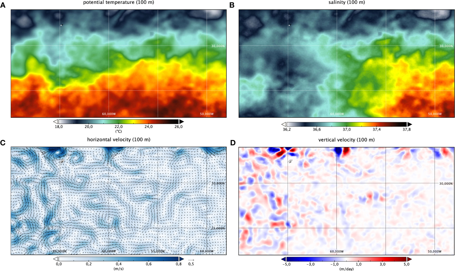
Figure 3 Potential temperature (A), salinity (B), horizontal (C) and vertical (D) velocities at 100 m depth on the 1st of April 2014. In (C) velocities are shown as vectors, and colour indicates intensity; in (D) upward (downward) velocities are indicated as positive (negative) values. Area of black dots illustrate relative density of A. anguilla, for all sampling stations used (as in Figure 1B).
3.2 Larval distribution as observed in 2014
European eel larvae were caught at almost all stations (Figure 1B). The abundances tended to be highest in central parts of the transects; in the vicinity of the northern frontal zone, however, the tendency is weak and abundances at neighboring stations could differ greatly (for transect 3, Figures 2J–L). Across all transects, the abundances remained at the same level, and a relatively high larval abundance of 0.061 m−2 was seen as far east as 53°W.
The average length of all larvae sampled was 13.5 mm, and the average age was estimated to 30 days since hatching; thus, average spawning time for the sampled larvae has been estimated to 28 February 2014 (Ayala and Munk, 2018). The smallest larvae, indicating the area of spawning, were mostly found at the southern part of transects (Figure 1C); however, some small larvae were also found in the northern areas of sampling.
3.3 Modeled larval dispersion
The modeled dispersion of larvae was mainly driven by the mesoscale activity in the Sargasso Sea. Processes tended to increase retention in the release area, but also led to a turbulent diffusive transport towards nearby regions (Figure 4). The resulting dispersal was generally isotropic. The net effect was of a relative high retention of particles in the spawning region, with approximately 40% of the particles still in the release area after 250 days (Figure 5). Westward advection was more evident in the region west of 65°W, which transported larvae from the spawning area towards the Gulf Stream after mid-May (Figure 4B). During the same period, larvae that originated in the central and eastern part of the spawning area followed different pathways including northern and eastern directions (Figure 4B). By the end of July (5 months after release time), the routes of those larvae were merging to the tracks of larvae of western origin, thus entering the Gulf Stream/North Atlantic Current at a more easterly site (Figure 4B). This pattern becomes more apparent through time (e.g., 8 months after release, Figure 4C). In the simulated period, larvae stemming from the eastern part of the spawning area were not found west of 70°W while they were transported south-, north-, or eastwards (Figure 4C).
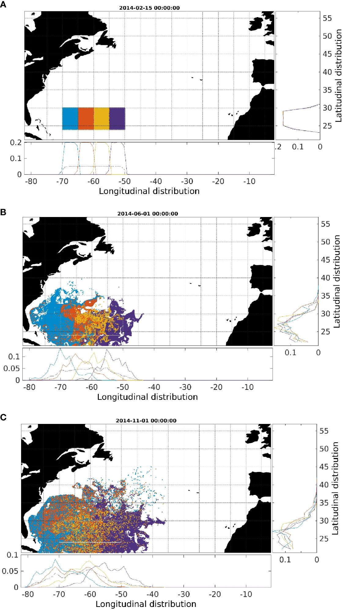
Figure 4 Simulated dispersion of eel larvae at different time periods in 2014 (A) assumed spawning time (February 15th) (B) first June (C) first November (end of the simulation). Different colors are used for different longitudinal release values. In the inset panels the longitudinal and latitudinal probability functions from the simulated particle distributions are displayed for the different colored groups.
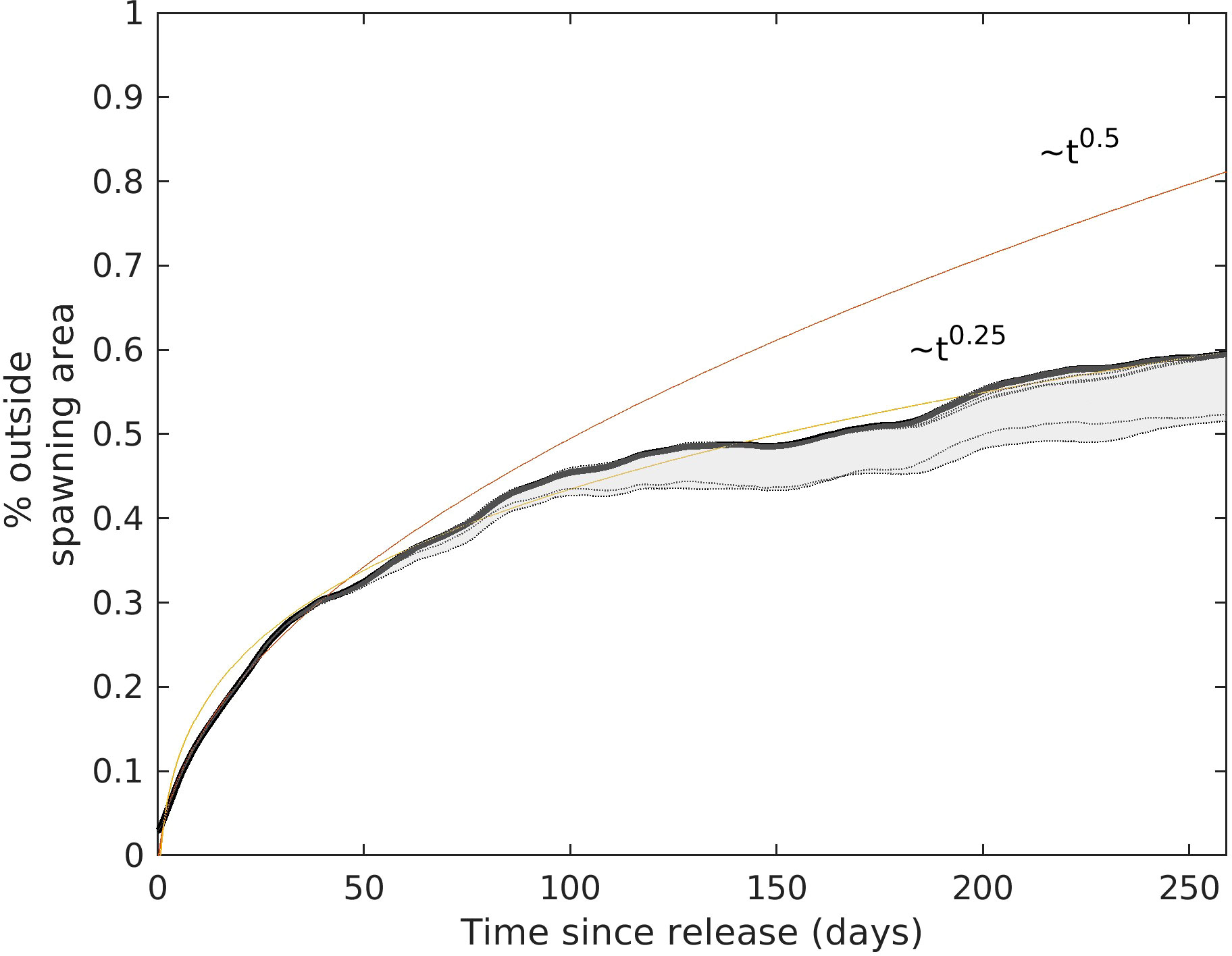
Figure 5 Fraction of larvae outside the spawning area as function of simulation time (in days). The fitting curves at t0.5 (red line) and t0.25 (purple line), are shown to compare with a pure diffusive transport. Shaded area indicates the range of the different curves obtained testing different parameters of the tracking algorithm. In total eleven models have been tested (dashed lines) with resulting curves with 1% deviation, but within 10% for models not including diel vertical migrations.
3.4 Comparison between modeled dispersion and historical data on larvae
The historical data on larval abundances, as contoured in Figure 6, show peak concentrations of larvae in the defined spawning area and towards northeast from there. Thus, at any time, only few larvae of the European eel were observed west of the spawning area. Specific observations of zero abundances of this species are available from the reported hauls containing American eel larvae. In a range of these hauls, there are no parallel presence of European eel, and this could thus be interpreted as “zero catch” of European eel. The dominance in the west-northwestern region of such negative hauls compared to positive hauls illustrates the relative scarcity of European eel larvae in this area (Figure 6, specific dots). Note in Figure 6 that we integrate all data, and the map is biased by uneven sampling intensity across areas and time of year; hence, the illustration should be considered with caution. A more detailed presentation and analysis of historical data are presented by Miller et al. (2015).
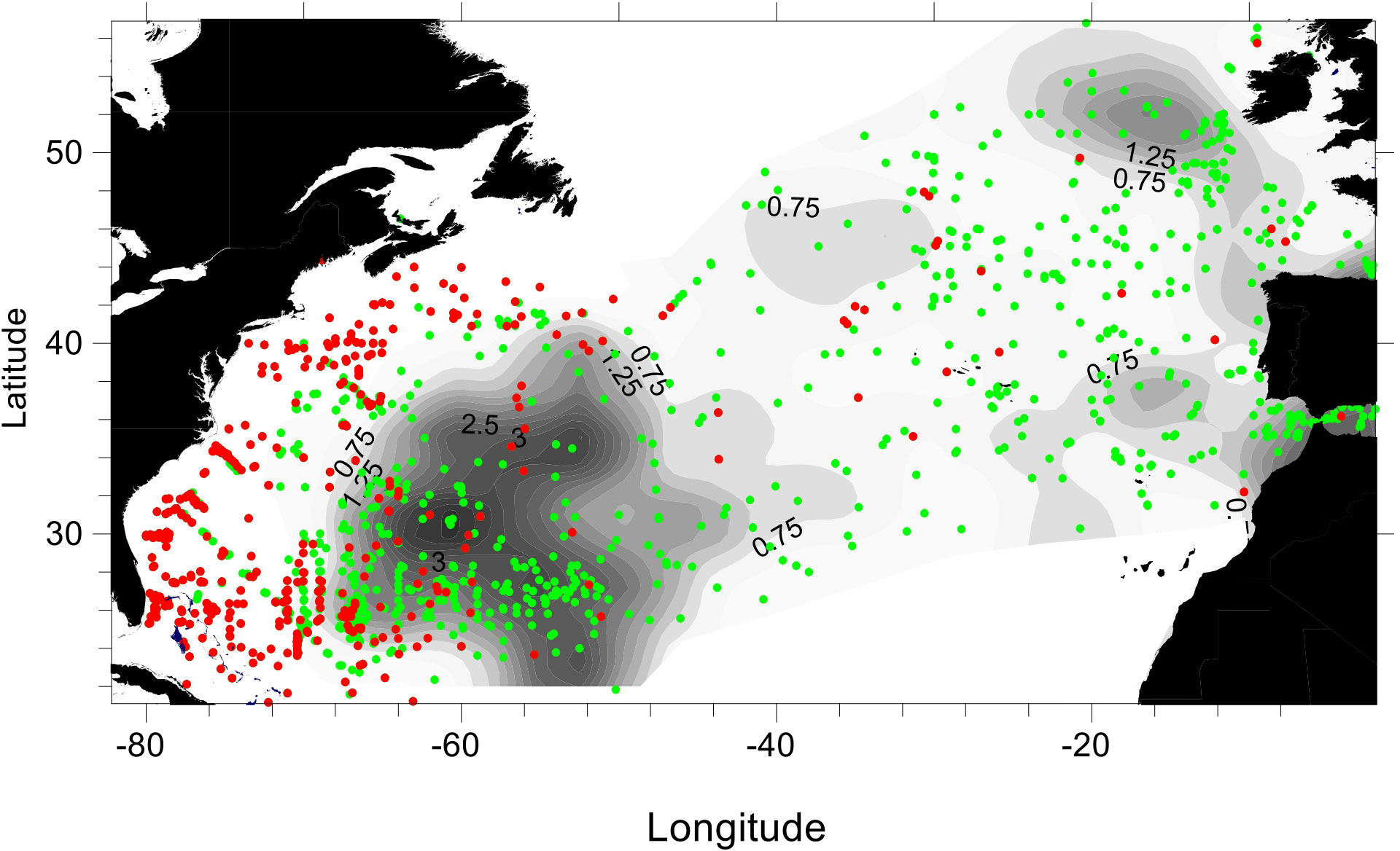
Figure 6 Overall abundance estimates of Anguilla anguilla larvae based on all sampling stations during the historical period (1914-2007). Shaded contouring of larval abundances (no per haul in intervals of 0.25, some labels illustrated). Green circles illustrate stations with A.anguilla presence; red circles illustrate other stations sampled where there was no catch of A. anguilla.. Note that contouring has included observations across all seasons during all years.
Average sizes of larvae in the historical database increased with distance from the central spawning area (Figure 7). The estimated increase in size appears quite monotonic towards north and east. As proposed by Schmidt (1922), spatial changes in average sizes of larvae would indicate directions of dispersal and drift. Larval average sizes do not show a trend of increase towards west within the spawning area, a pattern to be expected if there was a dominant initial westerly drift of all larvae from the spawning grounds. We compare this pattern with our modeled drift of larvae, illustrated by overlaid plots of age-specific distributions in Figure 7. This simulated dispersion by age shows some resemblance to the spatial trend apparent from observed average lengths. Note that the modeled regions in Figure 7 express the maximum range of larvae at any given time after release; hence, direct comparisons between ages and sizes cannot be made in this illustration.
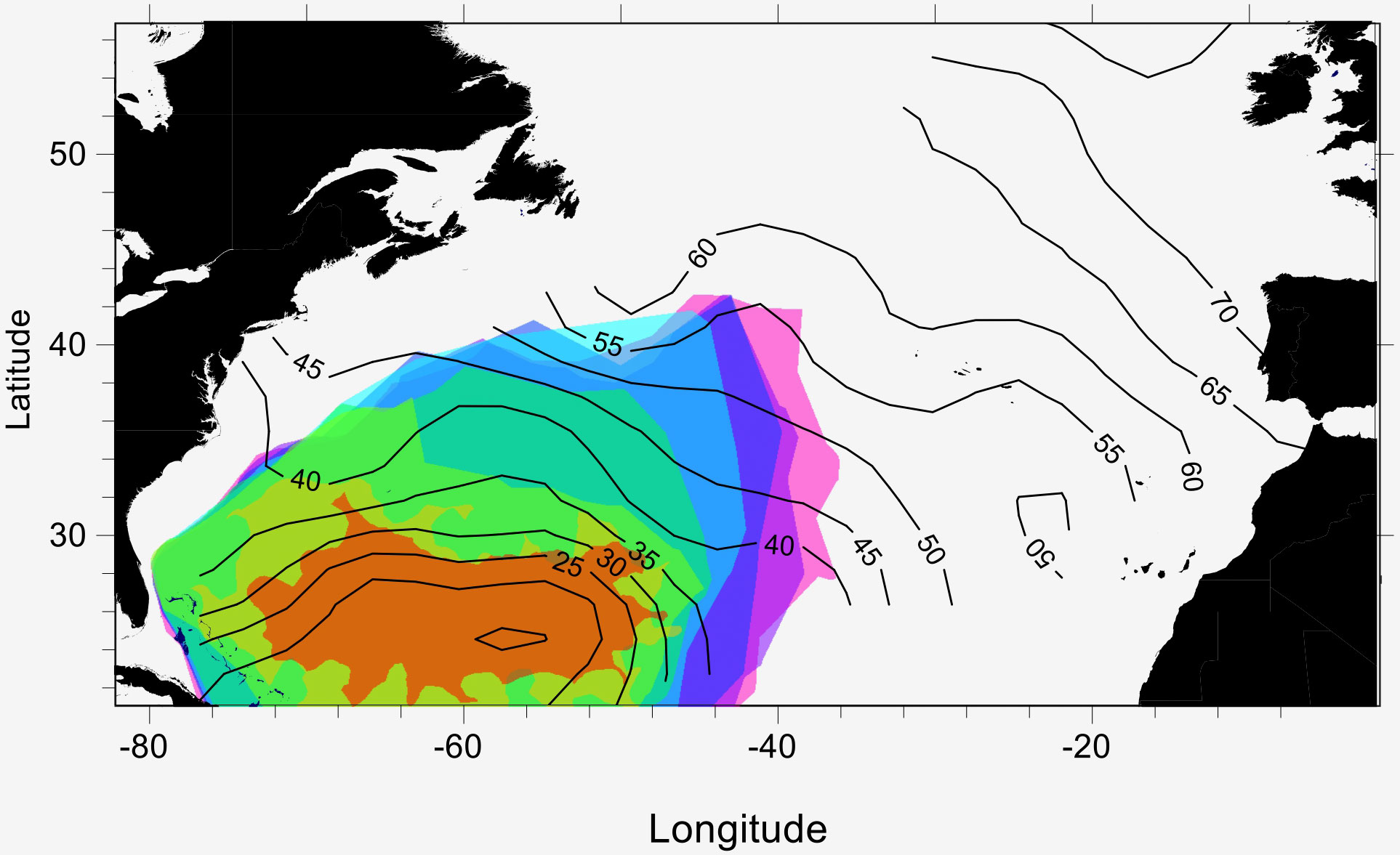
Figure 7 Age specific distributions of simulated Anguilla anguilla larvae overlaid contours of historical mean larval length distributions. Age distributions illustrated by colors: intervals of 30 days from brown (age 0-30 d) to pink (age 210-230 d). Contours of mean length are given in 5 mm intervals.
4 Discussion
4.1 Hydrography and transports in the STCZ
Hydrographic conditions in the study area were dominated by mesoscale eddies with typical length scales of ~100 km (Figure 1). Relatively strong eastward geostrophic currents of more than 0.15 m s−1 were observed in the upper 150 m along the frontal zones in the eddies, i.e., the separation of warm subtropical water masses from colder water of more northerly origin. General agreement between steric height anomalies, calculated from the upper 400 m, and estimates of sea level anomalies based on satellite observations indicated that the estimated geostrophic currents could represent the spatial variation in currents along the transects. The general eastward geostrophic current component in the frontal zones can be explained by the poleward decrease of temperature and the corresponding meridional pressure gradient in the upper water masses (Figures 2G–I).
Transient mesoscale eddies characterize the STCZ in all subtropical gyres (Ullman et al., 2007) and they represent a stable habitat mainly driven by the meridional temperature gradient between upper water masses in the tropics and extra-tropics (Halliwell et al., 1991). Analysis of the STCZ in the North Pacific showed general eddy activity throughout the year, albeit with a significantly more intense eddy activity during the spring period with a maximum in April/May (Qiu, 1999). Enhanced surface chlorophyll has been seen in areas of high eddy activity in the Sargasso Sea (Siegel et al., 2011). This can be explained by increased productivity and/or shallower pycnocline due to the passages of baroclinic eddies, as observed elsewhere (e.g., Johnson et al., 2010). Here, we find that the STCZ during the period of investigation (March to November 2014) has a slowly evolving mesoscale turbulent field with eddy-like structures very close to each other. These mesoscale features drive relatively slow vertical exchanges at the base of the euphotic layer (here taken as 100 m), associated with a semi-isotropic horizontal dispersion. The observed distribution of relatively large eastward currents associated with these mesoscale baroclinic eddy fields, and the simultaneous potential increase of biological production within the frontal zones (e.g., Mahadevan and Archer, 2000), may provide a suitable habitat and transport route for eel larvae across the subtropical gyre.
The largest eastward currents were observed in the upper 150 m, and this layer includes the deep chlorophyll maximum (DCM), which was observed to be a relatively constant feature in the study area located between 90 and 160 m depth (Richardson and Bendtsen, 2017). Eel larvae transported in these upper 150 m can thus find better feeding opportunities but also be subjected to potential threats from zooplankton grazing (e.g., Chang et al., 2018).
4.2 Larval dispersal modeling
To accurately assess the time-evolving lateral and vertical transport and dispersal of eel larvae from their spawning ground to their recruitment area, repeated synoptic observations of the 3D ocean state would ideally be required, as eel larvae are able to migrate vertically between approximately 50 m and 150 m depth. Unfortunately, direct observations providing such 3D ocean circulation time series cannot be achieved even when relying on the most advanced technologies. As a consequence, the sparse measurements collected from in situ platforms and surface-limited remote-sensing observations need to be combined with proper modeling frameworks to be able to infer the circulation in the ocean interior and provide realistic estimations of dispersion routes throughout the upper ocean layers. This can be done either by assimilating the observations within ocean general circulation numerical models (e.g., Stammer et al., 2016; Carrassi et al., 2018; Moore et al., 2019) or, as done here, by combining data-driven reconstructions and dynamical diagnostic tools. This second approach is commonly adopted to get robust estimations of the surface circulation (based on satellite altimeter data), but the development of data-driven 3D ocean state reconstructions has been recently gaining much interest, especially considering the possible adaptation of emerging machine learning methodologies (and physically informed deep learning) specifically to this aim (Guinehut et al., 2012; Mulet et al., 2012; Rio et al., 2016; Ubelmann et al., 2016; Lopez-Radcenco et al., 2018; Buongiorno Nardelli, 2020a; Yan et al., 2020; Fablet et al., 2021). In fact, both data assimilation in ocean general circulation models and data-driven models have their own strengths and flaws: the former guarantee a more consistent and complete description of the physics represented by the model, but often display significantly reduced capability to reproduce non-assimilated observations, as shown, for example, by Buongiorno Nardelli (2020b). The latter, generally providing reduced-space reconstructions and lower-order approximations of the dynamics (as in the retrieval of geostrophic currents from altimeter data), do instead often match independent observations much more closely (Mulet et al., 2012; Rio et al., 2016; Ubelmann et al., 2016; Buongiorno Nardelli, 2020b). Here, we thus exploit Lagrangian modeling based on data-driven high-resolution reconstructions as we believe it can better describe the eel larvae dispersion.
4.3 Larval drift
Larvae transport in the Sargasso area appeared mainly driven by turbulent processes regulated by the mesoscale dynamics in the region. The resulting diffusive dispersal was generally isotropic (Figure 4) although a weak westward advective component was evident in the western side of the spawning region (west of 65°W, Figure 4). The net effect was of a relative high retention of particles in the spawning region, with approximately 40% of the particles still in the release area after 250 days (Figure 5). A crude estimate of the total diffusivity (κ) in the spawning region was calculated using the mean-squared-distance (MSD) over the simulated period for all particles, which resulted in an average value of κ = 104 m2 s−1, comparable with estimates in the region obtained from satellite altimetry (Abernathey and Marshall, 2013) and ARGO floats (Cole et al., 2015). However, these rough estimates are likely overestimates of the actual diffusivity since they included the component of the advection-related transport, which could be filtered out by, for example, taking the center of mass of subgroup of particles within the spawning region.
Our results remain robust when altering various parameters of the particle tracking algorithm, such as background diffusivity, Smagorinsky constant, integration time step, and integration algorithm (e.g., second-order methods). These changes introduce a deviation of less than ±1% from the estimated 40% retention after 250 days of transport. It should be noted that we constrained DVM based on larval depth of distribution observed in day and night experiments during the present cruise (Munk et al., 2018). Nonetheless, we tested different DVM models with different daylight target depths (i.e., 60 m, 75 m, and 100 m) and results are consistent with the original model (deviation within ±1%, Figure 5). Larger changes in the results are obtained when DVM is not included and particles remain at constant depths (i.e., tested depths 50 m and 150 m). In these cases, approximately 10% less transport from the spawning area is obtained (shaded area in Figure 5).
An important aspect apparent in Figure 5 is that MSD scaled linearly over time, which points towards diffusive transport. This is regardless of the absolute value of diffusivity. The net effect of this mechanism was a relatively high retention of particles in the spawning region. We estimated that approximately 40% of the particles could still be within the release area after 250 days (Figure 5). These results are consistent with proposals that significant retention of eel larvae could take place in the Sargasso Sea during the first year of eel larval life (Westerberg et al., 2017). However, our simulations also pointed to significant dispersal in all directions from the spawning area. Importantly, they also illustrate transport towards east and north, where larvae could be entering regions of the Gulf Stream/North Atlantic Drift, patterns that have not been reported before in other modeling studies of the drift of European eel larvae.
4.4 Conclusion
The study demonstrates the potential of a data-driven modeling approach focusing on mesoscale dynamics and revealing previously overlooked European eel larvae dispersion dynamics. The findings illustrate extensive dispersion of larvae including dispersion in the northern and northeastern directions from the spawning ground. Thus, they challenge the common belief that during their early stages, the eel predominantly follow an anticyclonic drift, at first westwards towards the Antilles Current and subsequently into the Gulf Stream.
Data availability statement
The original contributions presented in the study are included in the article/supplementary material. Further inquiries can be directed to the corresponding author.
Ethics statement
The animal study was reviewed and approved by the Animal Welfare Committee of DTU Aqua, Technical University of Denmark, represented by chairman Senior researcher Niels Jepsen.
Author contributions
PMu had the lead of project, assembled field data, and over-viewed article writing, PMa and BN assembled data for modeling, made the analyses and wrote sections on the modeling. JB assembled, analyzed and considered the specific hydrographic data. All authors contributed to the article and approved the submitted version.
Acknowledgments
This study was supported by the Carlsberg Foundation, Denmark (2012_01_0272) and the Danish Centre for Marine Research (2013_02). PMa delivered this work under the MISSION ATLANTIC project, funded by the European Union’s Horizon 2020 Research and Innovation Program under grant agreement no. 639862428. PMa and BB acknowledge the contribution of the ESA World Ocean Circulation project (ESA Contract No. 4000130730/20/I-NB).
Conflict of interest
The authors declare that the research was conducted in the absence of any commercial or financial relationships that could be construed as a potential conflict of interest.
Publisher’s note
All claims expressed in this article are solely those of the authors and do not necessarily represent those of their affiliated organizations, or those of the publisher, the editors and the reviewers. Any product that may be evaluated in this article, or claim that may be made by its manufacturer, is not guaranteed or endorsed by the publisher.
References
Abernathey R. P., Marshall J. (2013). Global surface eddy diffusivities derived from satellite altimetry. J. Geophys. Res.: Oceans 118.2, 901–916. doi: 10.1002/jgrc.20066
Aoyama J. (2009). Life history and evolution of migration in catadromous eels (genus Anguilla). Aqua-BioSci Monogr. 2, 1–42.
Ayala D. J., Munk P. (2018). Growth rate variability of larval European eels (Anguilla Anguilla) across the extensive eel spawning area in the southern Sargasso Sea. Fisheries Oceanogr. 27 (6), 525–535. doi: 10.1111/fog.12273
Baltazar-Soares M., Biastoch A., Harrod C., Hanel R., Marohn L., Prigge E., et al. (2014). Recruitment collapse and population structure of the European eel shaped by local ocean current dynamics. Curr. Biol. 24 (1), 104–108. doi: 10.1016/j.cub.2013.11.031
Barceló-Llull B., Pascual A., Mason E., Mulet S. (2018). Comparing a multivariate global ocean state estimate with high-resolution in situ data: An anticyclonic intrathermocline eddy near the Canary Islands. Front. Mar. Sci. 5 (MAR). doi: 10.3389/fmars.2018.00066
Blanke B., Bonhommeau S., Grima N., Drillet Y. (2012). Sensitivity of advective transfer times across the North Atlantic Ocean to the temporal and spatial resolution of model velocity data: Implication for European eel larval transport. Dynamics Atmospheres Oceans 55, 22–44. doi: 10.1016/j.dynatmoce.2012.04.003
Bonhommeau S., Blanke B., Treguier A. M., Grima N., Rivot E., Vermard Y., et al. (2009). How fast can the European eel (Anguilla Anguilla) larvae cross the Atlantic Ocean? Fisheries Oceanogr. 18 (6), 371–385.
Buongiorno Nardelli B. (2013). Vortex waves and vertical motion in a mesoscale cyclonic eddy. J. Geophys. Res. Ocean. 118 (10), 5609–5624. doi: 10.1002/jgrc.20345
Buongiorno Nardelli B. (2020a). A deep learning network to retrieve ocean hydrographic profiles from combined satellite and in situ measurements. Remote Sens. 12 (19), 3151. doi: 10.3390/rs12193151
Buongiorno Nardelli B. (2020b). A multi-year timeseries of observation-based 3D horizontal and vertical quasi-geostrophic global ocean currents, Earth Syst. Sci. Data 12), 1711–1723. doi: 10.5194/essd-12-1711-2020
Buongiorno Nardelli B., Guinehut S., Pascual A., Drillet Y., Ruiz S., Mulet S. (2012). Towards high resolution mapping of 3-D mesoscale dynamics from observations. Ocean Sci. 8 (5), 885–901. doi: 10.5194/os-8-885-2012
Buongiorno Nardelli B., Guinehut S., Verbrugge N., Cotroneo Y., Zambianchi E., Iudicone D. (2017). Southern ocean mixed-layer seasonal and interannual variations from combined satellite and in situ data. J. Geophys. Res. Ocean. 122 (12), 10042–10060. doi: 10.1002/2017JC013314
Buongiorno Nardelli B., Mulet S., Iudicone D. (2018). Three-dimensional ageostrophic motion and water mass subduction in the southern ocean. J. Geophys. Res. Ocean. 123 (2), 1533–1562. doi: 10.1002/2017JC013316
Cabanes C., Grouazel A., von Schuckmann K., Hamon M., Turpin V., Coatanoan C., et al. (2013). The CORA dataset: validation and diagnostics of in-situ ocean temperature and salinity measurements. Ocean Sci. 9, 1–18. doi: 10.5194/os-9-1-2013
Carrassi A., Bocquet M., Bertino L., Evensen G. (2018). Data assimilation in the geosciences: An overview of methods, issues, and perspectives, Wiley Interdiscip. Rev. Clim. Change 9 (5), 1–50. doi: 10.1002/wcc.535
Chang Y. L. K., Miyazawa Y., Béguer-Pon M., Han Y. S., Ohashi K., Sheng J. (2018). Physical and biological roles of mesoscale eddies in Japanese eel larvae dispersal in the western North Pacific Ocean. Sci. Rep. 8, 5013. doi: 10.1038/s41598-018-23392-5
Cole S. T., Wortham C., Kunze E., Owens W. B. (2015). Eddy stirring and horizontal diffusivity from Argo float observations: Geographic and depth variability. Geophys. Res. Lett. 42 (10), 3989–3997. doi: 10.1002/2015GL063827
Cushman-Roisin B. (1984). On the maintenance of the subtropical front and its associated countercurrent, J. Phys. Oceanogr 14, 1179–1190. doi: 10.1175/1520-0485(1984)014<1179:OTMOTS>2.0.CO;2
Droghei R., Buongiorno Nardelli B., Santoleri R. (2018). A new global sea surface salinity and density dataset from multivariate observations, 1993–2016). Front. Mar. Sci. 5 (March). doi: 10.3389/fmars.2018.00084
Fablet R., Amar M. M., Febvre Q., Beauchamp M., Chapron B. (2021). End-to-end physics-informed representation learning for satellite ocean remote sensing data: Applications to satellite altimetry and sea surface currents. ISPRS Ann. Photogramm. Remote Sens. Spat. Inf. Sci. 5 (3), 295–302. doi: 10.5194/isprs-annals-V-3-2021-295-2021
Gaillard F., Autret E., Thierry V., Galaup P., Coatanoan C., Loubrieu T. (2009). Quality control of large Argo datasets. J. Atmos. Ocean Technol. 26 (2), 337–351. doi: 10.1175/2008JTECHO552.1
Guinehut S., Dhomps a.-L., Larnicol G., Le Traon P.-Y. (2012). High resolution 3-D temperature and salinity fields derived from in situ and satellite observations. Ocean Sci. 8 (5), 845–857. doi: 10.5194/os-8-845-2012
Halliwell G. R. Jr., Ro Y. J., Cornillon P. (1991). Westward-propagating SST anoMalies and baroclinic eddies in the Sargasso Sea. J. Phys. Oceanogr. 21, 1664–1680. doi: 10.1175/1520-0485(1991)021<1664:WPSAAB>2.0.CO;2
IOC, SCOR, IAPSO. (2010). The international thermodynamic equation of seawater – 2010: Calculation and use of thermodynamic properties. Intergovernmental Oceanographic Commission, Manuals and Guides No. 56, UNESCO (English), 196 pp.
Jacobsen M. W., Smedegaard L., Sørensen S. R., Pujolar J. M., Munk P., Jónsson B., et al. (2017). Assessing pre-and post-zygotic barriers between North Atlantic eels (Anguilla Anguilla and A. rostrata). Heredity 118 (3), 266–275. doi: 10.1038/hdy.2016.96
Johnson K. S., Riser S. C., Karl D. M. (2010). Nitrate supply from deep to near-surface waters of the North Pacific subtropical gyre. Nature 465, 1062–1065. doi: 10.1038/nature09170
Kettle A. J., Haines K. (2006). How does the European eel (Anguilla Anguilla) retain its population structure during its larval migration across the North Atlantic Ocean? Can. J. Fisheries Aquat. Sci. 63 (1), 90–106. doi: 10.1139/f05-198
Kimura S., Tsukamoto K., Sugimoto T. (1994). A model for the larval migration of the Japanese eel: roles of the trade winds and salinity front. Mar. Biol. 119 (2), 185–190. doi: 10.1007/BF00349555
Kleckner R. C., McCleave J. D. (1988). The northern limit of spawning by Atlantic eels (Anguilla spp.) in the Sargasso Sea in relation to thermal fronts and surface water masses. J. Mar. Res. 46 (3), 647–667.
Kracht R. (1982). On the geographic distribution and migration of I-and II-group eel larvae as studied during the 1979 Sargasso Sea Expedition. Helgoländer Meeresuntersuchungen 35 (3), 321–327. doi: 10.1007/BF02006140
Kuroki M., Miller M. J., Tsukamoto K. (2014). Diversity of early life-history traits in freshwater eels and the evolution of their oceanic migrations. Can. J. Zool. 92 (9), 749–770. doi: 10.1139/cjz-2013-0303
Lopez-Radcenco M., Pascual A., Gomez-Navarro L., Aissa-El-Bey A., Chapron B., Fablet R. (2018). Analog data assimilation of along-track nadir and wide-swath swot altimetry observations in the western Mediterranean Sea. IEEE J. Sel. Top. Appl. Earth Obs. Remote Sens. 12 (7), 2530–2540.
Mahadevan A., Archer D. (2000). Modeling the impact of fronts and mesoscale circulation on the nutrient supply and biogeochemistry of the upper ocean. J. Geophys. Res. Ocean 105, 1209–1225. doi: 10.1029/1999JC900216
Mason E., Pascual A., Gaube P., Ruiz S., Pelegrí J., Delepoulle A. (2017). Subregional characterization of mesoscale eddies across the Brazil-Malvinas Confluence. J. Geophys. Res. Ocean. 122 (4), 3329–3357. doi: 10.1002/2016JC012611
McCleave J. D. (1993). Physical and behavioural controls on the oceanic distribution and migration of leptocephali. J. Fish Biol. 43, 243–273. doi: 10.1111/j.1095-8649.1993.tb01191.x
Melià P., Schiavina M., Gatto M., Bonaventura L., Masina S., Casagrandi R. (2013). Integrating field data into individual-based models of the migration of European eel larvae. Mar. Ecol. Prog. Ser. 487, 135–149. doi: 10.3354/meps10368
Miller M. J., Bonhommeau S., Munk P., Castonguay M., Hanel R., McCleave J. D. (2015). A century of research on the larval distributions of the Atlantic eels: a re-examination of the data. Biol. Rev. 90 (4), 1035–1064. doi: 10.1111/brv.12144
Miller M. J., Westerberg H., Sparholt H., Wysujack K., Sørensen S. R., Marohn L., et al. (2019). Spawning by the European eel across 2000 km of the Sargasso Sea. Biol. Lett. 15 (4), 20180835. doi: 10.1098/rsbl.2018.0835
Moore A. M., Martin M. J., Akella S., Arango H. G., Balmaseda M., Bertino L., et al. (2019). Synthesis of ocean observations using data assimilation for operational, real-time and reanalysis systems: A more complete picture of the state of the ocean. Front. Mar. Sci. 6 (March). doi: 10.3389/fmars.2019.00090
Mulet S., Rio M.-H., Mignot A., Guinehut S., Morrow R. (2012). A new estimate of the global 3D geostrophic ocean circulation based on satellite data and in-situ measurements. Deep Sea Res. Part II Top. Stud. Oceanogr. 77–80, 70–81. doi: 10.1016/j.dsr2.2012.04.012
Munk P., Hansen M. M., Maes G. E., Nielsen T. G., Castonguay M., Riemann L., et al. (2010). Oceanic fronts in the Sargasso Sea control the early life and drift of Atlantic eels. Proc. R. Soc. B: Biol. Sci. 277 (1700), 3593–3599.
Munk P., Nielsen T. G., Jaspers C., Ayala D. J., Tang K. W., Lombard F., et al. (2018). Vertical structure of plankton communities in areas of European eel larvae distribution in the Sargasso Sea. J. Plankton Res. 40 (4), 362–375. doi: 10.1093/plankt/fby025
O’Connor B. M., Fine R. A., Olson D. B. (2005). A global comparison of subtropical underwater formation rates. Deep-Sea Res. 52, 1569–1590. doi: 10.1016/j.dsr.2005.01.011
Okubo A. (1970). Horizontal dispersion of floatable particles in the vicinity of velocity singularities such as convergences. Deep sea Res. oceanographic abstracts 17 (3), 445–454. doi: 10.1016/0011-7471(70)90059-8
Pacariz S., Westerberg H., Björk G. (2014). Climate change and passive transport of E uropean eel larvae. Ecol. Freshw. Fish 23 (1), 86–94. doi: 10.1111/eff.12048
Piollè, Autret (2023) Quality Information Document for SST TAC SST_GLO_PHY_L4_NRT_010_043 product, Ref: CMEMS-SST-QUID-010-043. Available at: https://catalogue.marine.copernicus.eu/documents/QUID/CMEMS-SST-QUID-010-043.pdf.
Pujol M.-I., Faugére Y., Taburet G., Dupuy S., Pelloquin C., Ablain M., et al. (2016). DUACS DT2014: the new multi-mission altimeter data set reprocessed over 20years. Ocean Sci. 12, 1067–1090. doi: 10.5194/os-12-1067-2016
Qiu B. (1999). Seasonal eddy field modulation of the North Pacific Subtropical Countercurrent: TOPEX/Poseidon observations and theory. J. Phys. Oceanogr. 29, 2471–2486. doi: 10.1175/1520-0485(1999)029<2471:SEFMOT>2.0.CO;2
Richardson K., Bendtsen J. (2017). Photosynthetic oxygen production in a warmer ocean: The Sargasso Sea as a case study. Phil. Trans. R. Soc. A. 375 (2102), 20160329. doi: 10.1098/rsta.2016.0329
Rio M. H., Santoleri R., Bourdalle-Badie R., Griffa A., Piterbarg L., Taburet G. (2016). Improving the altimeter-derived surface currents using high-resolution sea surface temperature data: A feasability study based on model outputs. J. Atmos. Ocean Technol. 33 (12), 2769–2784. doi: 10.1175/JTECH-D-16-0017.1
Schabetsberger R., Miller M. J., Olmo G. D., Kaiser R., Økland F., Watanabe S., et al. (2016). Hydrographic features of anguillid spawning areas: potential signposts for migrating eels. Mar. Ecol. Prog. Ser. 554, 141–155. doi: 10.3354/meps11824
Schmidt J. (1922). IV.—The breeding places of the eel. Philos. Trans. R. Soc. London Ser. B Containing Papers Biol. Character 211 (382-390), 179–208.
Schoth M., Tesch F. W. (1982). Spatial distribution of 0-group eel larvae (Anguilla sp.) in the Sargasso Sea. Helgoländer Meeresuntersuchungen 35 (3), 309–320. doi: 10.1007/BF02006139
SEA-MAT. (2022). Matlab Tools for Oceanographic Analysis. Available at: https://sea-mat.github.io/sea-mat/.
Siegel D. A., Peterson P., McGillicuddy D. J. Jr., Maritorena S., Nelson N. B. (2011). Bio-optical footprints created by mesoscale eddies in the Sargasso Sea. Geophys. Res. Lett. 38, L13608. doi: 10.1029/2011GL047660
Smagorinsky J. (1963). General circulation experiments with the primitive equations: I. The basic experiment. Monthly weather Rev. 91 (3), 99–164. doi: 10.1175/1520-0493(1963)091<0099:GCEWTP>2.3.CO;2
Stammer D., Balmaseda M., Heimbach P., Köhl A., Weaver A. (2016). Ocean data assimilation in support of climate applications: status and perspectives. Ann. Rev. Mar. Sci. 8 (1), 491–518. doi: 10.1146/annurev-marine-122414-034113
Ubelmann C., Cornuelle B. D., Fu L.-L. (2016). Dynamic mapping of along-track ocean altimetry: method and performance from observing system simulation experiments. J. Atmos. Ocean. Technol. 33, 1691–1699. doi: 10.1175/JTECH-D-15-0163.1
Ullman D. S., Cornillon P. C., Shan Z. (2007). On the characteristics of subtropical fronts in the North Atlantic. J. Geophys. Res. 112, C01010. doi: 10.1029/2006JC003601
Weiss J. (1991). The dynamics of enstrophy transfer in two-dimensional hydrodynamics. Physica D: Nonlinear Phenomena 48 (2-3), 273–294. doi: 10.1016/0167-2789(91)90088-Q
Westerberg H., Pacariz S., Marohn L., Fagerström V., Wysujack K., Miller M. J., et al. (2017). Modeling the drift of European (Anguilla Anguilla) and American (Anguilla rostrata) eel larvae during the year of spawning1. Can. J. Fisheries Aquat. Sci.
Keywords: European eel, dispersion, mesoscale, Sargasso Sea, larvae, survey, model
Citation: Munk P, Buongiorno Nardelli B, Mariani P and Bendtsen J (2023) Mesoscale-driven dispersion of early life stages of European eel. Front. Mar. Sci. 10:1163125. doi: 10.3389/fmars.2023.1163125
Received: 10 February 2023; Accepted: 17 July 2023;
Published: 08 August 2023.
Edited by:
Jinyu Sheng, Dalhousie University, CanadaReviewed by:
Kyoko Ohashi, Dalhousie University, CanadaShiliang Shan, Royal Military College of Canada (RMCC), Canada
Copyright © 2023 Munk, Buongiorno Nardelli, Mariani and Bendtsen. This is an open-access article distributed under the terms of the Creative Commons Attribution License (CC BY). The use, distribution or reproduction in other forums is permitted, provided the original author(s) and the copyright owner(s) are credited and that the original publication in this journal is cited, in accordance with accepted academic practice. No use, distribution or reproduction is permitted which does not comply with these terms.
*Correspondence: P. Munk, cG1AYXF1YS5kdHUuZGs=