Predicting the Loop Current dynamics combining altimetry and deep flow measurements through the Yucatan Channel

The Loop Current is the main mesoscale feature of the Gulf of Mexico oceanic circulation. With peak velocities above 1.5 m s^–1, the Loop Current and its mesoscale eddies are of interest to fisheries, hurricane prediction and of special concern for the security of oil rig operations in the Gulf of Mexico, and therefore understanding their predictability is not only of scientific interest but also a major environmental security issue. Combining altimetric data and an eddy detection algorithm with 8 years of deep flow measurements through the Yucatan Channel, we developed a predictive model for the Loop Current extension in the following month that explains 74% of its variability. We also show that 4 clusters of velocity anomalies in the Yucatan Channel represent the Loop Current dynamics. A dipole with positive and negative anomalies towards the western side of the Channel represents the growing and retracted phases respectively, and two tripole shape clusters represent the transition phases, the one with negative anomalies in the center associated with 50% of the eddy separation events. The transition between these clusters is not equally probable, therefore adding predictability. Finally, we show that eddy separation probability begins when the Loop Current extends over 1800 km (~27.2°N), and over 2200 km of extension, eddy detachment and reattachment is more frequent than separation. These results represent a step forward towards having the best possible operational Loop Current forecast in the near future, incorporating near real-time data transmission of deep flow measurements and high resolution altimetric data.

1 Introduction

The Gulf of Mexico is a sea in the North Atlantic that is about 1700 km wide, connected to the Caribbean Sea and the North Atlantic through the Yucatan Channel and Florida Straits, respectively. The Yucatan Channel is wider (200 km) and deeper (2040 m) than the Florida Straits, which is 150 km wide and about 1400 m deep between Havana and the Florida Keys, but only 800 m between Miami and Bimini, and its topography is also more complex (Sturges and Evans, 1983). In a very first approximation, at seasonal/annual scales, a mean of about 27.2 Sv enters the Gulf through the Yucatan Channel, as the Loop Current, and goes out into the North Atlantic through the Florida Straits (Candela et al., 2019).

The Loop Current is the main mesoscale dynamic feature of the Gulf of Mexico (Figure 1), having a major impact on the circulation and its variability (Leben, 2005). The Loop Current carries warm and saline Caribbean waters into the Gulf and sheds large anticyclonic eddies at irregular intervals, ranging from 6 to 12 months, with occasional longer shedding interval of 18 months (Sturges and Leben, 2000; Oey et al., 2003; Leben, 2005; Laxenaire et al., 2023). The eddy shedding is mostly driven by barotropic instability (e.g. Yang et al., 2023), and the retreat latitude of the Loop Current after an eddy shedding is linearly correlated with the time to the following shedding (Lugo-Fernández and Leben, 2010). Altimetric data allows to identify the Loop Current dynamics and also to identify and track the shedding of eddies (e.g. Hall and Leben, 2016). With peak velocities above 1.5 m s⁻¹, the Loop Current and its mesoscale eddies are of interest to many activities and of special concern for the security to oil rig operations in the Gulf of Mexico, particularly over the Sigsbee escarpment. Therefore understanding its predictability is not only of scientific interest but also a major environmental concern (National Academies of Sciences, Engineering, Medicine et al., 2018).

FIGURE 1

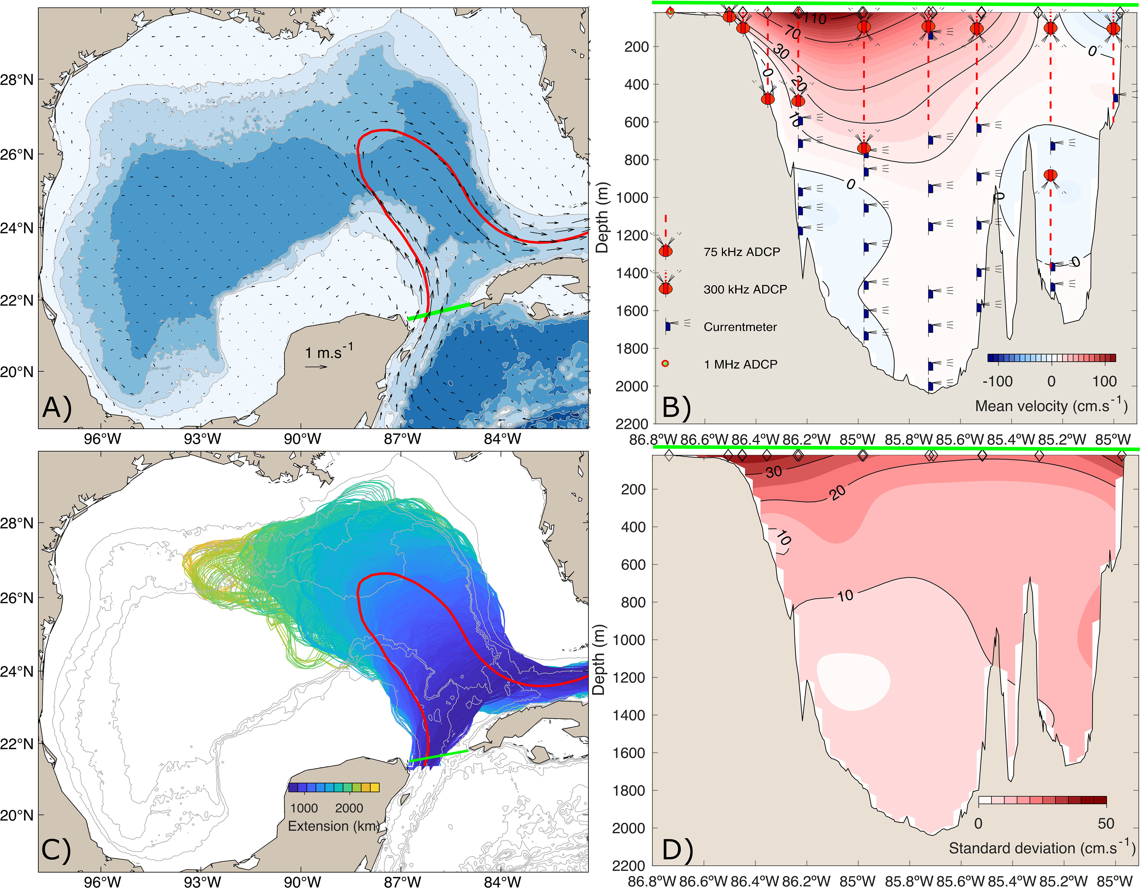
Figure 1 (A) Map of the Gulf of Mexico. Shaded colors show the bathymetry, while black vectors are the altimeter-derived mean geostrophic velocity. The Loop Current mean position also tracked from altimetry is shown in red, and the mooring array location in green. (B) Section of the Yucatan Channel. Shaded colors show the mean velocity through the channel (cm s⁻¹) computed from 8 years of gridded in-situ observations. The instruments used in each mooring are also sketched. Modified from (Candela et al., 2019). (C) Loop Current position in the Gulf of Mexico from 29 years of daily altimetry data. The color scale represents the extension (in km) of each day. The Loop Current mean position also tracked from altimetry is shown in red, and the mooring array location in green. (D) Standard deviation (cm s⁻¹) of the mean velocity across Yucatan Channel from 8 years of continuous in-situ observations from moorings as shown in (C).

The Yucatan Channel has been identified as a crucial section to monitor in order to understand and forecast the Loop Current extension/retraction processes and eddy shedding events (Reid, 1972; Candela et al., 2002; Sheinbaum et al., 2002; Athié et al., 2012; Hall and Leben, 2016; Hamilton et al., 2016). Given its relevance, mooring arrays have been deployed in the Yucatan Channel since 1999, in what is called the CANEK project (Ochoa et al., 2003). This mooring section allowed us to study the whole vertical and horizontal flow structure, its variability and its mean state over relatively long periods of time (Sheinbaum et al., 2002; Abascal et al., 2003; Athié et al., 2015; Candela et al., 2019). The main feature of the velocity field in the Yucatan section is the Yucatan Current, whose horizontal displacements are highly correlated with the first two principal components of the empirical orthogonal function (EOF) analysis applied to the velocity field (Abascal et al., 2003). Hence, these horizontal displacements of the Yucatan Current contribute the larger part of the variability along the entire section (Abascal et al., 2003; Candela et al., 2003; Sheinbaum et al., 2016; Athié et al., 2020). The characteristics of the flow variability through the Yucatan section present a relatively weak annual and semiannual cycle, explaining 19% and 32% of the transport variance respectively (Athié et al., 2020).

Previous modeling efforts suggest that both the surface and deep flow contribute to the predictability of the Loop Current (Oey, 1996; Vazquez et al., 2023), as it was proposed by Maul (1977), and tested later by Bunge et al. (2002) through observational in-situ and satellite data. Still, the predictability of the Loop Current evolution from the flow at the Yucatan Channel is far from well understood. Therefore, the objective of this manuscript is to use the in-situ observations of the flow variability through Yucatan Channel combined with altimetric data to understand and predict the Loop Current extension and eddy separation events.

2 Data

2.1 Gridded in-situ data: the CANEK database

We used an optimal interpolation product generated by Durante et al. (2023) from observational mooring array data. The dataset provides ocean currents (speed and direction) in the Yucatan Channel throughout the water column. The instrumentation on the moorings is a combination of Acoustic Doppler Current Profilers (ADCPs) and current meters in a configuration with up to ten moorings in the array as shown in Figure 1. The data cover the time period from July 2012 to July 2020, achieving more than 8 years with 99.9% of temporal coverage from hourly measurements. The mooring array was serviced approximately once per year, configurations changed slightly between deployments, and more moorings were added in the 2018-2020 period. See Candela et al. (2019) for details about each of the moorings deployments, instruments and configurations.

Before the spatial gridding procedure, standard processing and data quality management is carried out. Then, a gridding process is done using the optimal interpolation method (Bretherton et al., 1976; Roemmich, 1983). Gaussian spatial auto-correlation functions are implemented with decorrelation scales of 70 km and 500 m in the horizontal and vertical axis, respectively. Then, spatial mapping is performed onto a regular grid with 0.03°horizontal and 20 m vertical resolution at hourly time step. Daily means used here were computed from hourly means.

2.2 Satellite data

This study uses gridded satellite altimetry data distributed by Copernicus Marine Environment Monitoring Service. The data are the DT-2018 version from the Ssalto/Duacs multi-mission processing system that combines observations from multiple satellite missions (Capet et al., 2014; Pujol et al., 2016; Ballarotta et al., 2019), and gridded in space and time to 0.25° horizontal and daily temporal resolution. Here, the properties of absolute dynamic topography and derived surface geostrophic velocity are used, and the study area encompasses the entire Gulf of Mexico over the period 1993–2021.

3 Methods

3.1 Loop Current metrics and mesoscale eddies detection

Loop Current identification and metrics were computed using two different methods: The first one, following Hamilton et al. (2000) and widely used since then (e.g. Leben, 2005; Gopalakrishnan et al., 2013), consists of tracking the 0.17 m sea level contour connecting the Yucatan Channel with the Florida Straits in the Gulf after removing data outside the Gulf and the daily spatial mean as a way to eliminate the effect of homogeneous surface heating (from now on, the 0.17 m method). Some of the output metrics are the Loop Current extension (length measured in km), and northward (°) and westward (°) maximum extensions (Figures 1, 2).

FIGURE 2

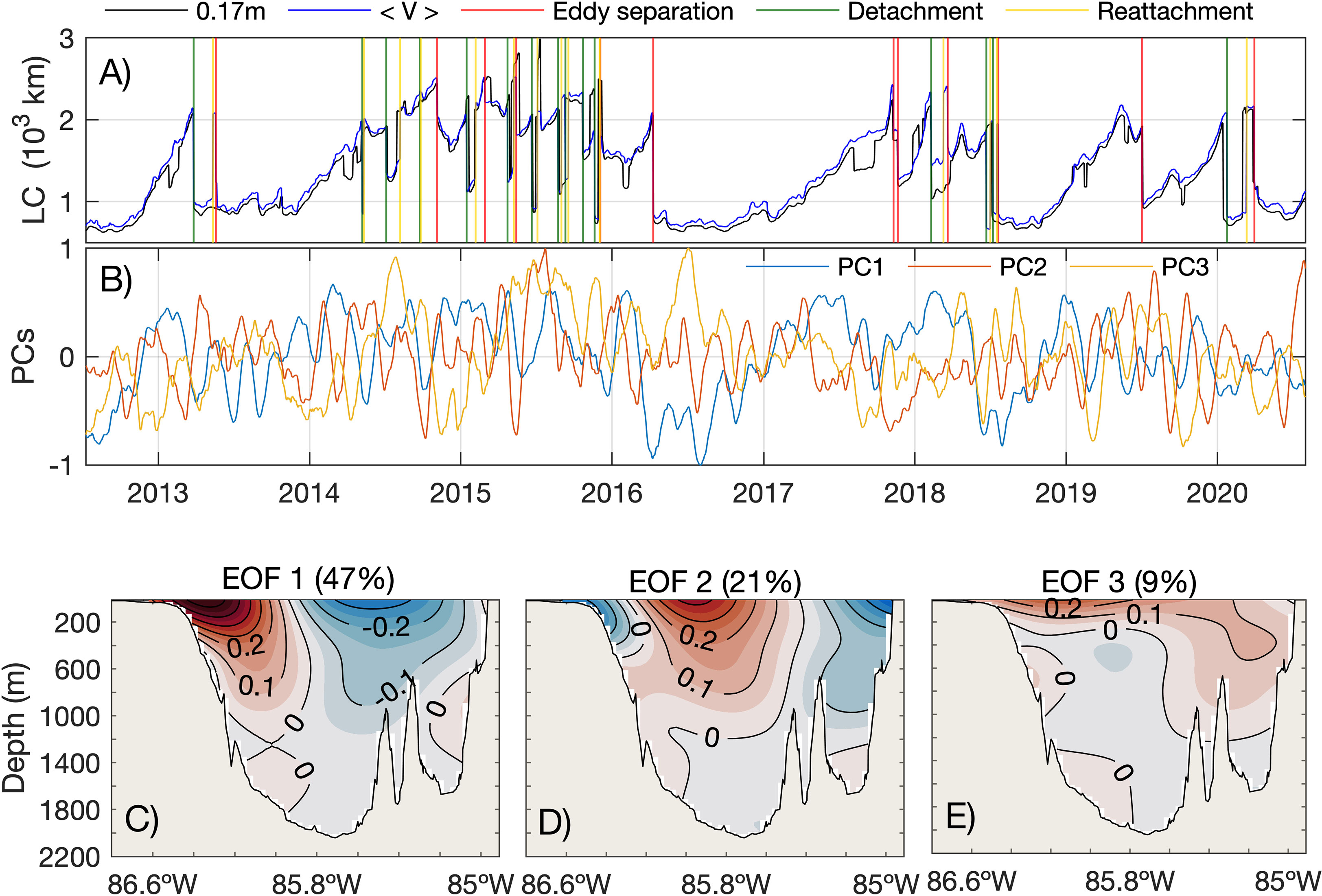
Figure 2 (A) Time-series of the Loop Current extension (km) from two different methods. The 0.17 m contour method is colored in black and the maximum gradient method in blue. Vertical red lines show each time an eddy was separated from the Loop Current, while green and yellow show detachment and reattachment events, respectively. (B) Empirical orthogonal function analysis of the in-situ flow measurements through the Yucatan Channel. The lines show the first 3 Principal Components, while (C, D, E), the spatial structure of the EOFs, with the explained variance on top.

The second method to identify the Loop Current was developed by Laxenaire et al. (2023). It consists of tracking the sea level streamline associated with maximum geostrophic velocity that connects the Yucatan Channel to the Straits of Florida (from now on, the <V> method). According to the authors, the method ensures that the Loop Current enters and exits the Gulf of Mexico and is more objective. Also, we noticed that it is more robust to unrealistic abrupt changes due to interruptions in the 0.17 m contour (Figure 2).

The method by Laxenaire et al. (2023) also provides an eddy detection algorithm named TOEddies (Chaigneau et al., 2011; Pegliasco et al., 2015; Laxenaire et al., 2018) and therefore, quantitative information on the eddies’ interaction with the Loop Current. The TOEddies algorithm is also altimetry based and tracks enclosed streamlines of absolute dynamic topography, assuming geostrophic balance. It has been validated by comparing it with other eddy detection algorithms (e.g. Chelton et al., 2011) and in-situ observations from drifters (Lumpkin, 2016). The centers of the eddies are identified as extrema of the absolute dynamic topography, and the largest closed streamlines correspond to the boundary of these eddies. The eddy contour associated with the maximum azimuthal velocity, used as the eddy boundary in this study, is also identified. The eddies detected each day are then linked by trajectories if there is a superposition of the surface occupied by them between two time steps. This superposition method, developed by Pegliasco et al. (2015), allows the identification of merging and splitting of eddies.

Following Leben (2005), eddy shedding events by the Loop Current are classified into two groups: an eddy detachment is followed by a reattachment to the Loop Current, while an eddy separation is defined as the final detachment of an eddy from the Loop Current with no later reattachment. In Laxenaire et al. (2023), a comparison is made between the eddy separations obtained by this TOEddies and with respect to the method by Hall and Leben (2016), obtaining very similar results. A detailed description of the algorithm for the detection of eddies and the Loop Current extension can be found in Laxenaire et al. (2018) and Laxenaire et al. (2023), respectively.

3.2 in-situ data, smoothing and comparison with altimetry

A 21-day low-pass filter was applied to the interpolated mooring data product, in order to have a consistent time resolution between the mooring measurements and the effective time resolution of the altimeter used to detect the Loop Current (Ballarotta et al., 2019). The window for the low-pass filter was selected by finding the maximum correlation between altimetry and the different centered moving mean windows of the in-situ data (Figure 3). Then, the moving average window was applied to the mooring data using the current day and the previous 21 days in order to make this applicable to prediction using real-time data.

FIGURE 3

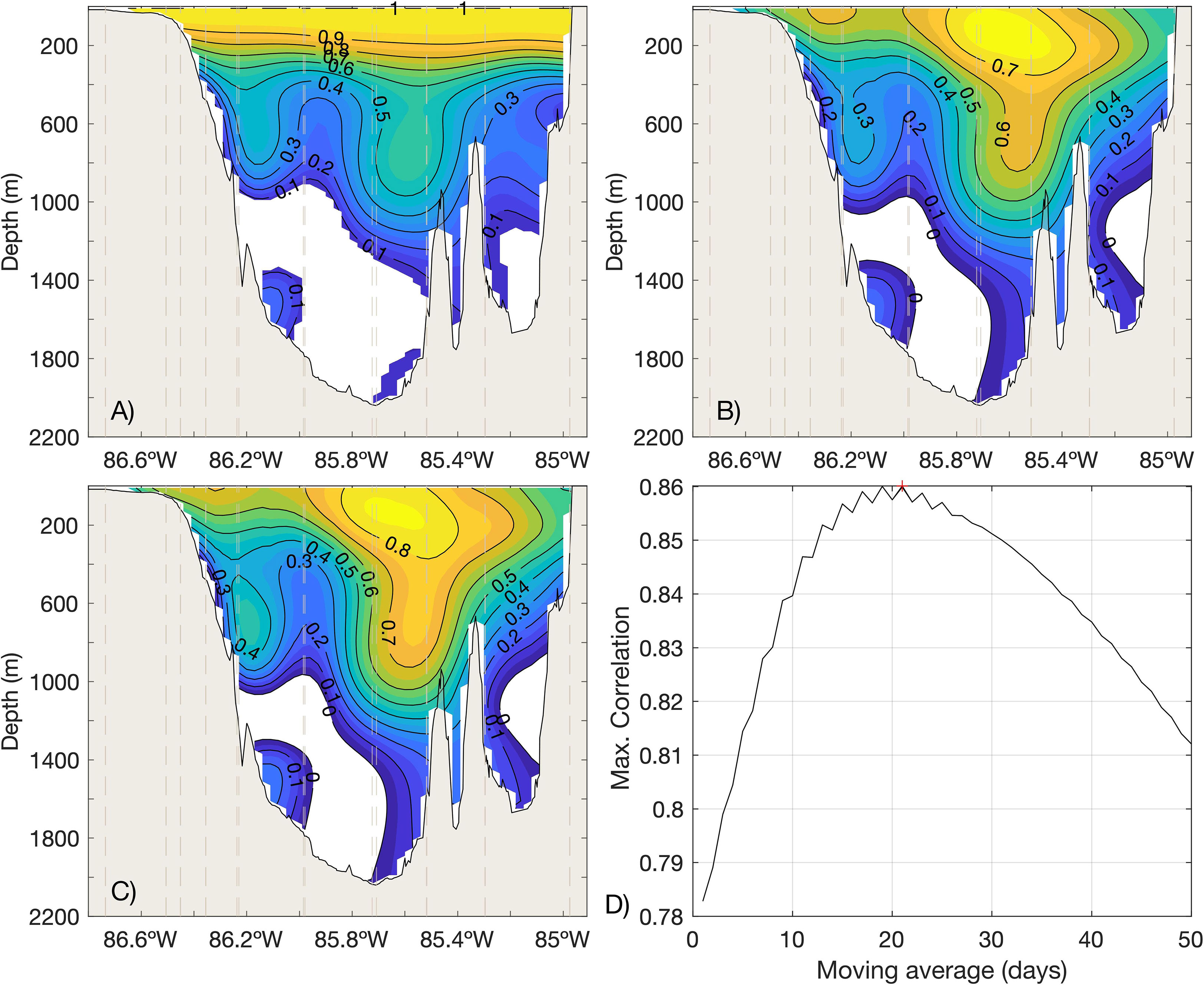
Figure 3 Pearson correlation coefficient for the linear regression between each gridded point from in-situ current measurements and: (A) co-located surface in-situ measurements (i.e. with the surface current at the same longitude), (B) the closest altimetric surface velocity data point, and (C) the closest altimetric data with a 21-day moving mean. (D) Maximum Pearson correlation coefficient with altimetry as a function of the low pass filtering of the in-situ data.

To estimate the correlation between mapped mooring velocities and altimetry derived geostrophic surface velocities, we first interpolated the altimetry data (25 km horizontal resolution) into the Yucatan section grid (5 km horizontal resolution) and rotated the vectors 10° anticlockwise in order to obtain the velocity through the channel. Then, we computed a linear regression between the interpolated across-channel altimetry geostrophic velocity and the mooring velocity product at each longitude point and over the entire water column, applying an independent linear regression at each depth point. The result was plotted as a section of the Pearson correlation coefficient (r). The same analysis was applied for the mooring surface velocity with all the water column data points at each longitude in order to compare the vertical extension of the correlation from the mooring product and altimetry derived geostrophic approximation. Statistical significance of all correlation pairs was tested with a Student T-test (α=0.01).

3.3 Empirical orthogonal function (EOF) and cluster analyses

With the objective of understanding the spatio-temporal variability of the flow through the Yucatan Channel and its relationship with the Loop Current extension and eddy shedding, EOF and cluster analyses were computed from the 8 years of through-channel gridded mooring velocity anomalies. The anomalies were calculated by subtracting the long term mean, as there were no substantial differences to removing the seasonal mean. EOFs were scaled by dividing/multiplying by the maximum value of the Principal Components (PCs) in order to obtain nondimensional PCs ranging from -1 to 1 and EOF maps with m s^–1 units. For clustering, the Ward method was used to generate the clusters, although other methods were tested too, with results being robust (e.g. using k-means). The Ward method prioritizes coherence within groups by minimizing the sum of variances within-groups (Wilks, 2011). 2944 days of observations were used, with a total of 3231 variables (grid points with data), and 4 clusters were retained. With the time-series of the clustering, we also constructed a Markov chain transition model to analyze the probability transition between the clusters through time. Clustering and their transition probability is a common technique used in atmospheric and ocean sciences to describe and predict for example weather regimes (e.g. Arizmendi et al., 2022).

3.4 Predictive model of the Loop Current and eddy shedding

The predictive model of the Loop Current extension was constructed by implementing a multiple linear regression, optimizing the lowest root mean square error (RMSE) between the observed and predicted time-series and retaining only statistically significant variables as predictors. The model was trained with the first two thirds of the data (5.3 years) in order to test it with the last third (2.7 years). Four input variables capture the main changes of the flow associated with the predictability of the Loop Current extension. Two of the predictive variables of the model are the meridional component of surface geostrophic velocity from altimetry averaged in the areas defined by those points above the 99.5 percentile and those below the 0.05 percentile on the Pearson correlation map between the Loop Current extension and meridional velocity, respectively. Averaging these areas with 13 grid points each provided better skill than any single point. The other 2 predictive variables were taken from the gridded velocity product by automatically identifying the points of maximum and minimum correlation in the Yucatan section at different depths, and then retaining only the points that actually contributed to improve the skill of the model by being more correlated with the Loop Current extension than with surface altimetry at that Longitude. Finally, we selected the best compromise of vertically aligned points in what could be a mooring array. The analysis was repeated for every time interval, and the selected model was the one with highest correlation and lag, which turned out to be 30 days.

Accurately predicting an eddy separation event with at least one month lead time represents a major challenge, as it depends not only on the Loop Current but also on the evolution of the mesoscale field of the Gulf of Mexico. Here, two analyses were carried out that contribute to the eddy separation predictability. The first one was analyzing the relative frequency of the Loop Current extension during all days and only during those days before an eddy separation or detachment took place. The second analysis consisted in determining the probability of an eddy separation or detachment depending on the cluster configuration of the flow anomalies in Yucatan Channel.

4 Results

4.1 Descriptive analysis of the Loop Current and Yucatan flow

The Loop Current metrics show similar results from the two different methods of the 0.17 m contour and the streamline associated with maximum velocity (<V>), with a mean extension of 1449 and 1495 km and standard deviation of 487 and 466 km, respectively (Figures 1C; 2A). Even though the time-series are very similar, the correlation is 0.86, thus explaining 74% of the variance, and a root mean square error (RMSE) of 262 km between the two time-series is observed.

The events identified by the eddy detection algorithm are marked in Figure 2A. This shows that almost all the abrupt changes in the Loop Current extension (e.g. >100km/10 days) are associated with eddy shedding events (separation, detachment or reattachment). Apart from detachment and reattachment events, the Loop Current shows a repeated cycle in which it grows slowly from a retracted phase (<1000km) until it reaches an extended phase of about 1800-2600 km, when an eddy separation occurs and the system goes back to the retracted phase. This cycle can take between some months and up to 2 years (Figure 2A).

TOEddies detected 48 separation events between 1993 and 2021, 12 within the overlap period with in-situ measurements made on 2013/5/20, 2014/11/5, 2015/2/28, 2015/5/15, 2015/12/4, 2016/4/9, 2017/11/10, 2017/11/21, 2018/3/21, 2018/7/21, 2019/7/3, and 2020/3/30. Also, 56 detachment/reattachment events were detected by TOEddies during the altimetric period, and 15 overlapped with the gridded product in the Yucatan Channel. All the gridded total velocities and velocity anomalies on the Yucatan Channel, and the altimetric maps with the Loop Current and eddy detection can be seen in the Video S1.

The flow through the Yucatan Channel is dominated by the Yucatan Current, represented by the intense northward flow West of 85.4°W, with a maximum mean velocity at the surface of 1.14 m s⁻¹ decaying to 0 m s⁻¹ at about 800 m (Figure 1B). Below 800 m, the system shows velocities close to 0 m s⁻¹ and mostly southward, although the standard deviation exceeds the mean (0.05-0.1 m s⁻¹). Close to the surface, the standard deviation increases with a maximum over the western slope (>0.3 m s⁻¹; Figure 1D), as seen in earlier studies (Sheinbaum et al., 2002; Athié et al., 2015; Candela et al., 2019).

Three EOFs explain 77% of the variance of the Yucatan flow across the Channel. The first EOF explains 47% of the variance and shows a dipole structure centered at about 86°W, with surface values up to 0.6 m s⁻¹ near the surface, decaying to almost 0 m s⁻¹ at 1000 m depth (Figures 2B, C). The second EOF has a similar vertical structure, but it is a tripole and explains 21% of the variance (Figure 2D). These first two EOFs are associated with the westward-eastward displacements of the Yucatan Current, as already reported by (Abascal et al., 2003), who identified the first two EOFs as a “propagating signal” connected to the meandering and movement of the Yucatan Current core across the Yucatan Channel. The third EOF explains 9% of the variance and is the only one of the three with a change of sign in the vertical structure, especially well defined where the core of the Yucatan Current is located at 86.1°W, describing changes in the baroclinicity of the current (Figure 2E). The first EOF is the only one significantly correlated with the 206 Loop Current extension (r=0.44).

4.2 In situ data, smoothing and comparison with altimetry

Gridded velocities through Yucatan Channel show over 0.95 correlation with the currents below everywhere in the upper 100 m section, decaying uniformly to a correlation of 0.5 at 400 m depth. A portion of this vertical auto-correlation is explained by the gridding method. Below 400 m, considerable zonal differences are observed with two regions of relatively high vertical correlation at 85.4°W and 86.2°W above 0.4 and two regions of relatively low correlation below 0.2 at 86° W and East of 85.2°W. Below 1000 m, no significant correlation is observed essentially where the mean flow is negative on both sides of the channel except for a small region at about 1400-1800 m at 86°W, where a weak significant correlation exists (Figure 3A).

Altimetry-derived geostrophic velocity through the Yucatan Channel is significantly correlated with the surface gridded mooring velocities and shows a similar vertical correlation structure. The main difference observed in the upper 200 m with respect to the gridded mooring data correlation is that the Pearson coefficient values are about 0.1-0.2 lower, and also that zonal differences are observed in the upper layers, with higher correlations observed at 85.5°W and 86.1°W and decreasing towards the shelf at both boundaries, reaching values below 0.6 at the surface. Another difference between the correlation with surface in-situ measurements and with altimetry derived velocities is that the maximum correlation between altimetry and the gridded mooring product is not observed at the surface, but at 190 m depth. Between 400 and 1000m of depth, the correlation of in-situ measurements with altimetry is higher than with in-situ surface measurements (Figures 3B, C). The maximum correlation (0.86) is found after applying a 21 day running mean to the gridded data (Figure 3D).

4.3 Yucatan flow anomalies during growth, eddy separation, and retracted phase

The results of the cluster analysis of the velocity anomalies are shown in Figure 4. The composites of the 4 clusters show a similar anomaly structure to the positive and negative phases of the first two EOFs. Clusters 2 and 4 have similar structure as the first EOF, a dipole with positive and negative anomalies oriented west-east for phase 4, and east-west for phase 1. The top panel shows that they are associated with a retracted and a growing phase of the Loop Current, respectively (Figure 4A, Table 1). Clusters 1 and 3 have similar structure as the second EOF, a tripole with a centered positive anomaly and negative anomalies towards the sides for the cluster 1, and the opposite for the cluster 3 (Figures 4B, D). These clusters are associated with the shift between phases 2 and 4, as they have more transitions and are less persistent than clusters 2 and 4 (Table 1).

FIGURE 4

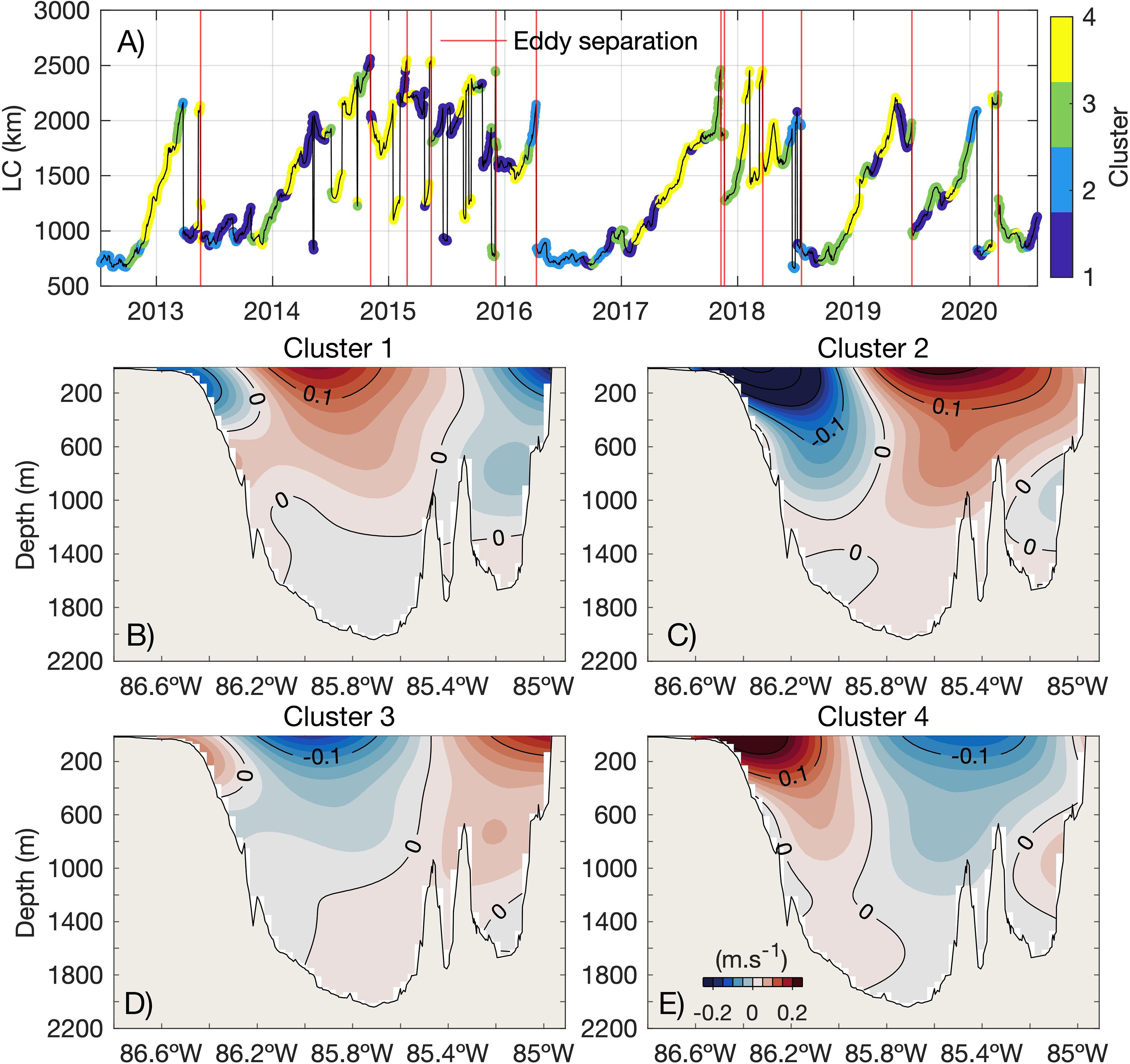
Figure 4 (A) Loop Current extension (km) time-series (in black) during the period with moorings in the Yucatan Channel. Each color in the time-series represents the corresponding cluster during that period based on the flow anomalies through the Yucatan Channel. Vertical red lines show each time an eddy was separated from the Loop Current. The composite of the velocity anomalies (m s^-1) of each cluster is plotted in (B–E).

TABLE 1

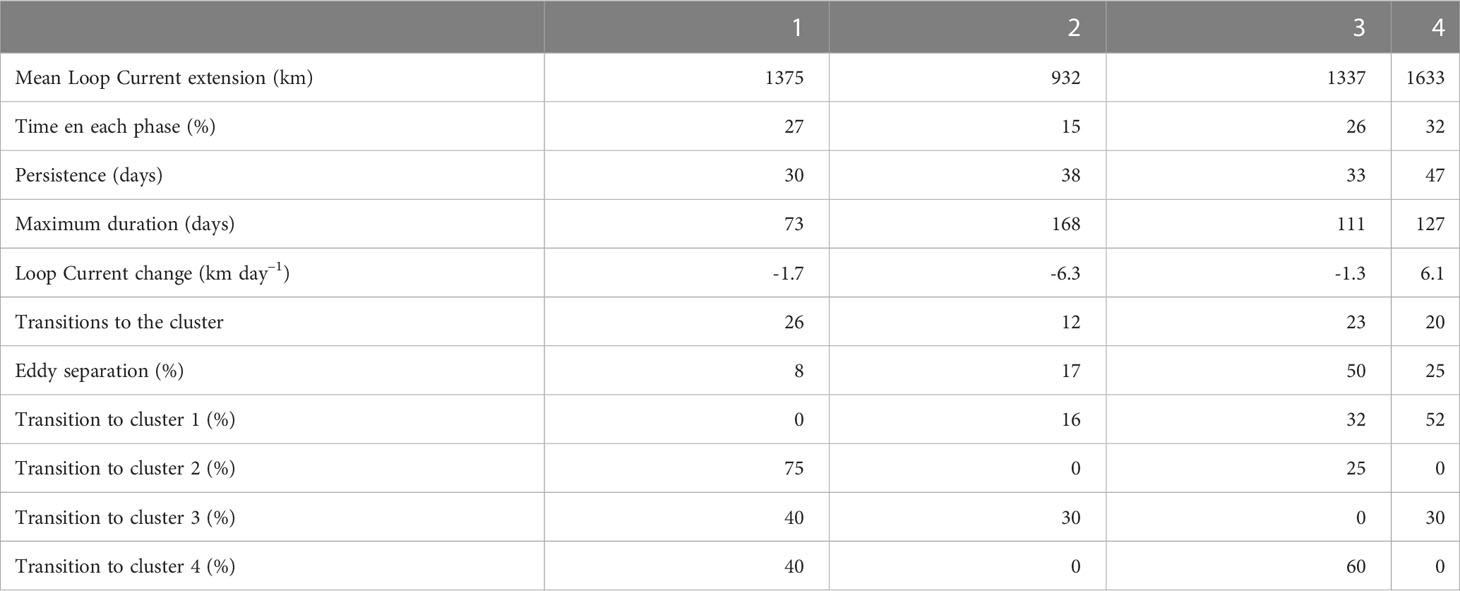
Table 1 Descriptive statistics of the four clusters based on velocity anomalies through the Yucatan Channel.

Descriptive statistics of the clusters show relevant results: Cluster 4, hereinafter also called the growing phase, is the one associated with the largest mean extension of the Loop Current (1633 km), and the only one with a positive net mean growth of the Loop Current, about 6.1 km day^–1 (Table 1). Cluster 2, hereinafter also called the retracted phase, stands out as the one associated with the lowest mean extension of the Loop Current (932 km), and the phase with the least transitions (12). Both clusters 2 and 4 are the most persistent ones, with a mean duration of 38 and 47 days, respectively (Table 1).

Clusters 3 and 1 are the transition clusters, being the less persistent ones. Nonetheless, cluster 3 is more frequent than the retracted phase of cluster 2, as the Loop Current often alters between cluster 3 and 4 during the extended phase before changing to the retracted phase of cluster 2 (e.g. 2014 to 2016 in Figure 4A). Cluster 3 is also the one with highest probability of eddy separation. 50% of the separations occur during cluster 3 while it is present 26% of the time (Table 1). Both transition clusters can represent a weakening or a strengthening of the Yucatan Current depending on whether the system is shifting from the retracted phase towards the growth phase or vice versa. Markov chain analysis indicates that these are not equally probable, and that cluster 1 is more associated with the transition from the retracted towards the extended phase (Table 1). Markov chain transition probability also shows that no transition is observed between cluster 2 (retracted phase) and 4 (extended phase).

The most probable cycle beginning from the retracted phase is towards Cluster 1, then to the growing phase and then to cluster 3. cluster 3 shows a very similar transition probability towards the other three clusters. Due to this last part of the loop phases 3 and 4 are where the most time is spent, even if 2 and 4 are the ones with more persistence. The retracted phase, although persistent, is the one with the least transitions, so the system alters frequently between the growing and transition phases and sometimes migrates towards the retracted phase after a separation event (Figure 4B, Table 1).

4.4 Predicting the Loop Current extension and eddy shedding

Horizontal (from altimetry) and vertical section (from Yucatan Channel mapped observations) distributions of the Pearson correlation coefficient between the Loop Current extension and the flow at each grid point 30 days before are shown in Figure 5. Both the horizontal map and the Yucatan Channel section display a dipole pattern, with positive correlation westward of the middle of the Yucatan Channel and negative towards the East. For the altimetric field, maximum and minimum correlation are observed downstream of the Yucatan Channel (> |0.6|), decaying northward of 25°N (Figure 5A).

FIGURE 5

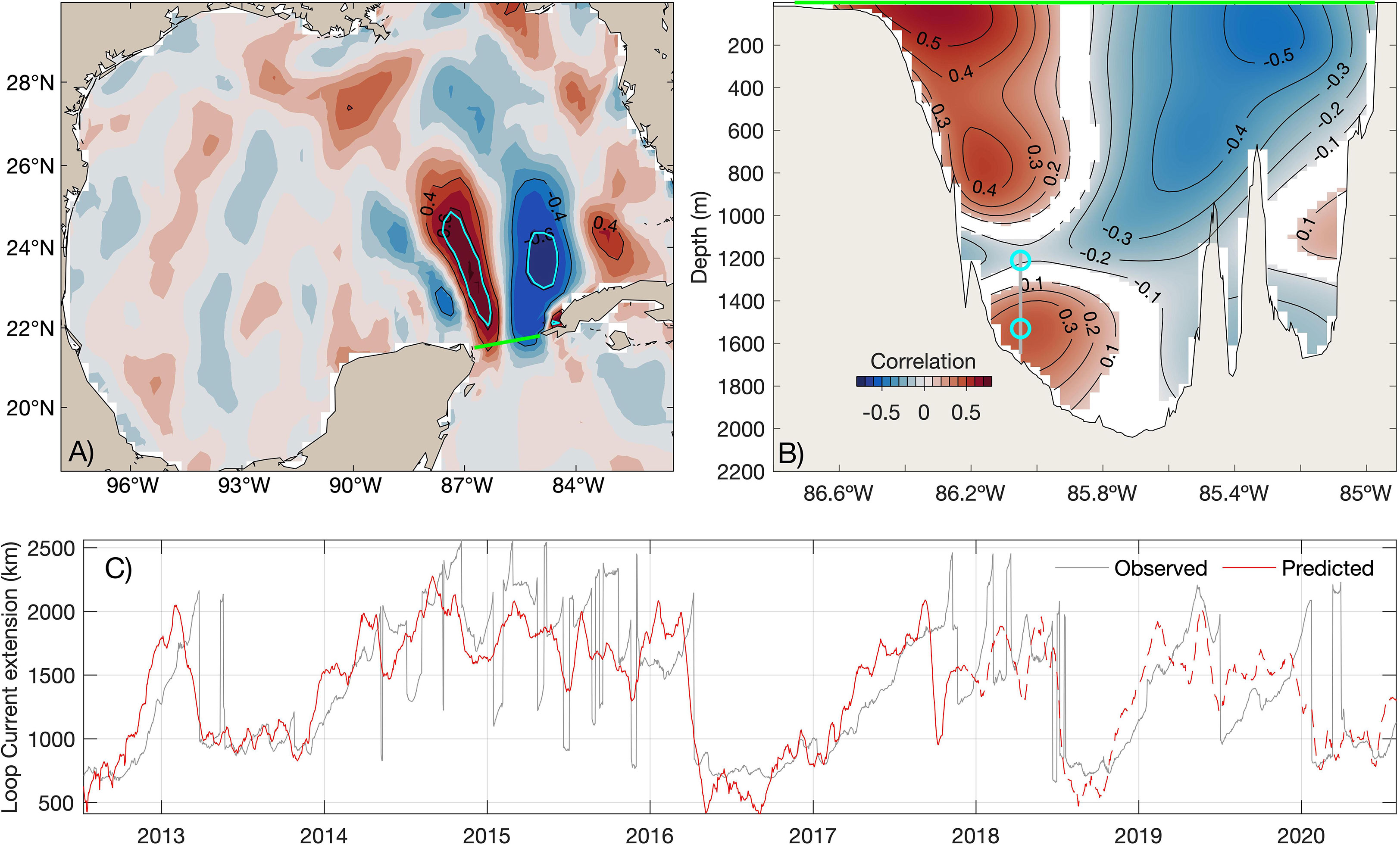
Figure 5 (A) Pearson correlation coefficient for the linear regression between meridional geostrophic velocity from altimetry at each grid point and the Loop Current extension one month later. Green lines in panels (A, B) represent the Yucatan Section. (B) Same as (A), but for gridded observations of velocity through Yucatan Channel. In both panels cyan signs show the areas used as input for the model. (C) Observed (gray) and predicted (red) loop current extension from the multiple linear regression model. Dashed red line shows the period where the corresponding observations where not considered for the prediction.

Maximum and minimum correlation values in the Yucatan Channel are observed near the surface (> |0.5|). The vertical extension of the correlation in the Yucatan Channel with respect to the surface is about 1000 m. Although it tends to decrease towards the deep, this is not the case at every longitude. For example, at 86.2°W, the upper 1000 m show positive correlation, with relative maxima from the surface to 800 m deep. The correlation sign does not change through the water column for each longitude point in most for the channel, except for the mid depths (1000-1400 m) at the boundaries. In particular, the negative correlation at this depth implies that as the Yucatan Current extends it not only shifts westward but also gets shallower. Below 1400 m the correlation shows the same sign as at the surface, with a relative maximum at 1530 m 86.05°W of 0.38 (Figure 5B).

A multiple linear regression model, based on the first 2/3 of the data record, explains 74% of the variance of the Loop Current extension (km) 30 days ahead (t₃₀), and a RMSE of 338 km, using four input variables as in equation 1:

$\begin{array}{ll}LC(t_{30},km)=1100+369v_1-579v_2+2403v_3-2946v_4& (1)\end{array}$

where all predictors are in m s^-1 and at t₀ v1 and are v2 are the altimetric geostrophic velocity averaged over the region above the 99.5 and below the 0.05 percentile of highest/lowest correlation, respectively (marked with a cyan line in Figure 5A), and v3 and v4 are the in-situ velocities at 1170 m and 1530 m deep Yucatan Channel at 86.1°W, marked with cyan circles in Figure 5B.

The Loop Current extension is well predicted during the growth and retracted phases, and generally also when there is a large drop in the Loop Current extension associated with an eddy separation. Both drops of July 2018 and January 2020 are due to the separation of large eddies and are captured by the model despite the fact that the gridded mooring data for the last third of the measurement period (Dec 2017 to August 2020) were not considered for estimating the regression coefficients. In the entire period the model fails to accurately predict the detachment and reattachment of eddies (Figure 5C).

A tipping point related to eddy shedding probability is observed when the Loop Current extends 1800 km. This is the most frequent extension of the Loop Current that is reached during the growth/charge phase, and also where the shedding events start to be probable, as almost no separation or detachment is observed at extensions below 1800 km. 1800 km corresponds to a maximum northern reach of the Loop Current at 27.3°N, as the interval 600 km (24°N) - 2100 km (28°N) shows a linear increase of about 375 km of the Loop Current extension for every 1 degree increase in the maximum northern extent. The separations and detachments are also significantly different in their occurrence probability according to the Loop Current extension. At ranges between 1800 and 2300 km, the separation is more probable, while above 2300 km a detachment/reattachment is more probable (Figure 6). At extensions over 2100 km, the Loop Current has usually reached the shelf break of the Northern Gulf of Mexico and starts to extend mostly westward (Figure 1C). Over 56% of the shedding events are reattached, while 46% are actually separations and lose contact forever with the Loop Current. 50% of the reattachments occurs within the first 12 days, and 95% within the first 2 months.

FIGURE 6

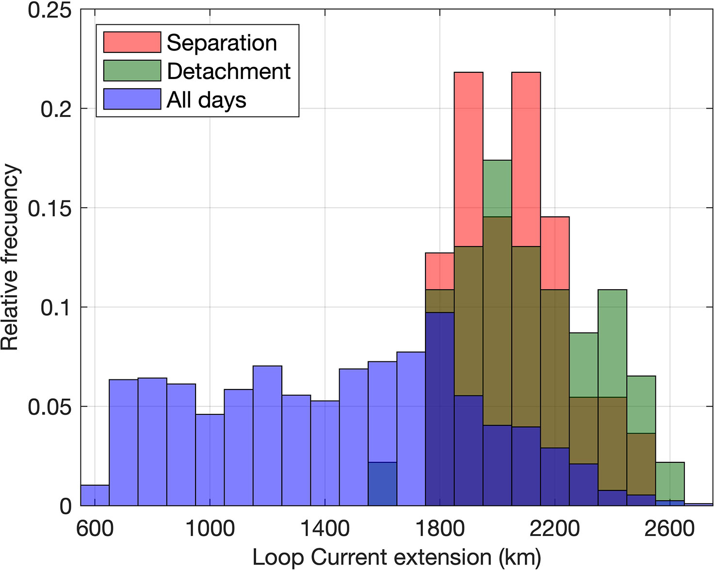
Figure 6 Relative frequency of the Loop Current extension for all days (blue), the days before a separation event (red), and detached events (green).

The flow anomalies through Yucatan Channel can also give predictability for the eddy separation and detachment, not only by predicting the Loop Current extension. Cluster 3, a tripole with negative anomalies in the core of the Yucatan Current, is observed prior to the separation events in 50% of the cases, although cluster 3 represents 26% of the time, and therefore it is more probable to observe a separation event when the Loop Current is over 1800 km of extension and shifts to Cluster 3. This is consistent with the results by Athié et al. (2012, 2015) who report an eastward shift of the Yucatan Current core prior to several eddy separations.

5 Discussion and conclusions

The deep flow measurements through the Yucatan Channel combined with altimetry data predict the Loop Current extension with a correlation of 0.86. The remaining unexplained variance, 26%, is of similar magnitude as the difference between the two Loop Current extension detection methods used. Therefore, correctly identifying the Loop Current extension probably is as important for its predictability as improving the predictive model.

Our results are consistent with previous research. Vazquez et al. (2023) showed that assimilating subsurface observations from moorings and altimetry significantly improved the model hindcasts and forecasts for the Loop Current extension, and also the eddy detachment. Bunge et al. (2002) demonstrate that filtering the deep transport time-series at Yucatan Channel with a 20 day running mean increases the correlation with the Loop Current extension by 0.21 with a lag of 8.5 days. Zeng et al. (2015) used an artificial neural network approach and an EOF decomposition of altimetry data to predict the Loop Current evolution and the shedding of an Loop Current eddy four weeks in advance, as in this research.

Our results are also consistent with (Wang et al., 2019; Wang et al., 2021), who also used machine learning to predict the Loop Current evolution and Loop Current Eddy shedding events with satisfactory results up to 12 weeks in advance. Chiri et al. (2019) implemented auto-regressive logistic regression models to predict the evolution of 8 Loop Current patterns, using as input data bi-weekly averages of altimetry data but also wind stress curl in the Gulf of Mexico, and in the Caribbean Sea, and sea level pressure anomalies over the North Atlantic. For a specific case for the year 2016, the authors managed to predict the Loop Current pattern evolution 3 months in advance. This 1 to 3 months window of predictability fits the operational scope for the objectives of the phase 3 of the Understanding Gulf Ocean Systems program (UGOS-3), and one challenge for the near future will be to combine the published approaches and datasets in order get the best possible predictability skill of the Loop Current extension and eddy shedding.

The main strength of the predictive model developed here is identifying the regions that have high forecast skill, firstly from altimetry, and then adding those deep flow measurements that effectively contribute to improve the predictability. Another strength of the predictive model is that the deep flow measurements can be reduced to a few locations which could be locations of moored observations, away from the near-surface intense flow that represents a challenge for operational mooring arrays. This is of particular interest for the objectives of one of the UGOS-3 projects, where pressure-sensing inverted echo sounders (PIES) transmitting data in real-time will be tested in the Yucatan Channel for deep flow observations.

The smoothing of the in-situ data to match the effective temporal resolution of the altimetry improved the predictability of the Loop Current. Maximum correlation with altimetry was not found in the upper layers where ageostrophic currents are considerable, but below 100 m depth, as observed in other regions (e.g. Manta et al., 2022). As a consequence of the altimetric detection of the Loop Current, a resulting limitation of this analysis is that the potential contribution of the higher frequencies (e.g. variability within two weeks) from in-situ data cannot be used.

High-frequency predictability implies also a challenge due to the limited resolution of the altimetric data, especially for predicting the detachment/reattachment events when the Loop Current is highly extended (>2000km) reaching north of 26°N. Although the Loop Current extension itself can act as a predictor, these events seem to be driven mainly by mesoscale eddy interactions in the North of the Gulf of Mexico, rather than by substantial changes in the flow anomalies in the Yucatan Channel over the previous weeks. However, this is a subject of intense discussion in the community since many detachments and separations have been linked with perturbations (eddies) coming from the Caribbean (Abascal et al., 2003; Athié et al., 2012; Athié et al., 2015; Sheinbaum et al., 2016). Predicting trajectories of the cyclonic eddies that constrain the Loop Current using TOEddies or any related eddy tracking algorithm could contribute to improve the predictability of these detachment/reattachment events in the future, especially if the upcoming data from the SWOT satellite allows us to better resolve the small cyclonic structures. As has been shown in previous studies, cyclonic eddies in the Gulf of Mexico can either block the growth of the Loop Current or favor the shedding of anticyclonic eddies from the Loop Current (Schmitz, 2005; Chérubin et al., 2006; Zavala-Hidalgo et al., 2006; Sheinbaum et al., 2016). A similar behavior has been identified for the Kuroshio Loop Current in the Luzon Strait (Zhang et al., 2017), making this region interesting to compare with in the future. Even though we are still not able to predict the detachment/reattachment events, we were able to show that the probability of an eddy separation or detachment/reattachment depends on the Loop Current extension which we can predict one month in advance, and that a tripole shape anomaly in the Yucatan Channel with negative values in the center of the Channel is observed before a separation event in 50% of the cases (Figure 7).

FIGURE 7

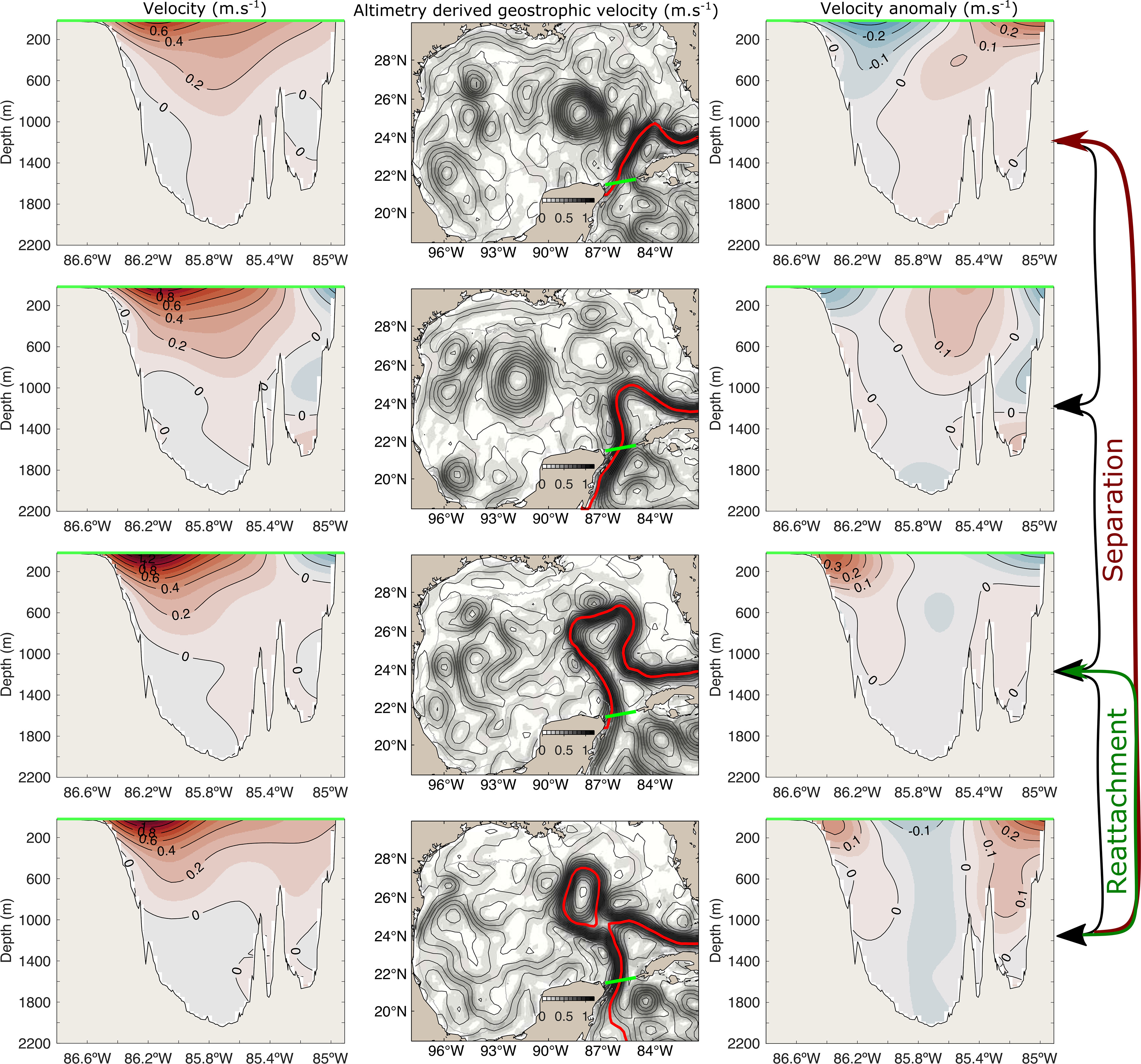
Figure 7 Schematic figure of the Loop Current evolution and eddy separation. Each row is a snapshot representative of each cluster (2, 1, 4 and 3 from top to bottom, respectively) of the through-channel flow anomalies in the Yucatan Channel constructed from the mean of the previous 21 days. The anomalies are plotted in the right columns, while the mean flow on the left columns. The columns of the center show the altimetry derived geostrophic velocity for the selected day, with the Loop Current colored in red. Green lines in all panels represent the Yucatan Section.

5.1 Conclusions

● We developed a predictive model of the Loop Current extension explaining 74% of the variance combining altimetry data and deep flow measurements at 1530 m and 1210 m deep in the Yucatan Channel at 86°W.

● 4 clusters of velocity anomalies through the Yucatan Channel represent the Loop Current dynamics. A dipole with positive and negative anomalies towards the western side of the Channel represents the growing and retracted phase of the Loop Current, and two tripole-shaped clusters represent the transition phases, with the one with negative anomalies in the center associated with 50% of the eddy separation events. The transitions between these clusters are not equally probable, thereby adding predictability.

● Eddy shedding probability begins when the Loop Current extends over 1800km, at which time it is situated near the slope in the northern Gulf. Beyond 2200 km extension, topography limits the direction of growth to mostly towards the west, and detachment and reattachment of eddies becomes more frequent than an eddy separation with other methods.

● Altimetry-derived geostrophic velocities are significantly correlated with in-situ flows in Yucatan Channel in the upper 1000 m. Nevertheless, high frequency (less than 2 weeks) events are not properly resolved by altimetry, making in-situ measurements not only of the deep flow but also the upper flow valuable to sample.

● These results will hopefully help to better resolve and predict the Loop Current dynamics in an operational way in the near future, once near real-time data of deep flow derived from the UGOS-3 project and high resolution altimetry from the SWOT satellite mission are available.

Data availability statement

The CANEK dataset is online and available on https://zenodo.org/record/7865542. Requests to access these datasets should be directed to CANEK.CICESE@gmail.com.

Author contributions

All authors contributed to the conception, design of the study and writing. GM also did the analysis and most of the writing. GD also did the Yucatan Channel data processing. All authors contributed to the article and approved the submitted version.

Funding

Research reported in this publication was supported by the Gulf Research Program of the National Academies of Sciences, Engineering, and Medicine under award numbers 2000011057 and 200013145. Funding of the gridded data base used in this study comes from CICESE internal funds. Partial funding also comes from the National Council of Science and Technology of Mexico, Mexican Ministry of Energy, Hydrocarbon Trust, project 201441, as part of the Gulf of Mexico Research Consortium (CIGoM).

Acknowledgments

The data set used in this study was generated by JC, P.I. of the CICESE-CANEK Project for more than 25 years, who sadly passed away in November 2022. He was a wonderful human being and an outstanding scientist who contributed ideas and work that made this study possible. We wish to dedicate this article in his memory.

Conflict of interest

The authors declare that the research was conducted in the absence of any commercial or financial relationships that could be construed as a potential conflict of interest.

Publisher’s note

All claims expressed in this article are solely those of the authors and do not necessarily represent those of their affiliated organizations, or those of the publisher, the editors and the reviewers. Any product that may be evaluated in this article, or claim that may be made by its manufacturer, is not guaranteed or endorsed by the publisher.

Author disclaimer

The content is solely the responsibility of the authors and does not necessarily represent the official views of the Gulf Research Program or the National Academies of Sciences, Engineering, and Medicine.

Supplementary material

The Supplementary Material for this article can be found online at: https://www.frontiersin.org/articles/10.3389/fmars.2023.1156159/full#supplementary-material

Supplementary Video 1 | Left panel show the flow through the Yucatan Channel, and the right panel the anomalies. Both are the average of the previous 21 days. The middle panel shows the evolution of absolutedynamic topography in the Gulf of Mexico. Red line shows the tracked Loop Current extension, while magenta and cyan contours show the tracked anticyclonic and cyclonic eddies, respectively. The title of the middle panel also shows the date and the Loop Current extension for that day.

References

Abascal A., Sheinbaum J., Candela J., Ochoa J., Badan A. (2003). Analysis of flow variability in the yucatan channel. J. Geophysical Research: Oceans 108. doi: 10.1029/2003JC001922

CrossRef Full Text | Google Scholar

Arizmendi F., Trinchin R., Barreiro M. (2022). Weather regimes in subtropical south america and their impacts over uruguay. Int. J. Climatology 42, 9253–9270. doi: 10.1002/joc.7816

CrossRef Full Text | Google Scholar

Athié G., Candela J., Ochoa J., Sheinbaum J. (2012). Impact of Caribbean cyclones on the detachment of loop current anticyclones. J. Geophysical Research: Oceans 117. doi: 10.1029/4052011JC007090

CrossRef Full Text | Google Scholar

Athié G., Sheinbaum J., Candela J., Ochoa J., Pérez-Brunius P., Romero-Arteaga A. (2020). Seasonal variability of the transport through the Yucatan channel from observations. J. Phys. Oceanography 50, 343–360. doi: 10.1175/jpo-d-18-0269.1

CrossRef Full Text | Google Scholar

Athié G., Sheinbaum J., Leben R., Ochoa J., Shannon M. R., Candela J. (2015). Interannual variability in the Yucatan channel flow. Geophysical Res. Lett. 42, 1496–1503. doi: 10.1002/2014GL062674

CrossRef Full Text | Google Scholar

Ballarotta M., Ubelmann C., Pujol M.-I., Taburet G., Fournier F., Legeais J.-F., et al. (2019). On the resolutions of ocean altimetry maps. Ocean Sci. 15, 1091–1109. doi: 10.5194/os-15-1091-2019

CrossRef Full Text | Google Scholar

Bretherton F. P., Davis R. E., Fandry C. (1976). A technique for objective analysis and design of oceanographic experiments applied to MODE-73. In Deep Sea Res. Oceanographic Abstracts 23, 559–582. doi: 10.1016/0011-7471(76)90001-2

CrossRef Full Text | Google Scholar

Bunge L., Ochoa J., Badan A., Candela J., Sheinbaum J. (2002). Deep flows in the Yucatan channel and their relation to changes in the loop current extension. J. Geophysical Research: Oceans 107, 26–1–26–7. doi: 10.1029/2001JC001256

CrossRef Full Text | Google Scholar

Candela J., Ochoa J., Sheinbaum J., López M., Pérez-Brunius P., Tenreiro M., et al. (2019). The flow through the gulf of Mexico. J. Phys. Oceanography 49, 1381–1401. doi: 10.1175/jpo-d-18-0189.1

CrossRef Full Text | Google Scholar

Candela J., Sheinbaum J., Ochoa J., Badan A., Leben R. (2002). The potential vorticity flux through the Yucatan channel and the loop current in the gulf of Mexico. Geophysical Res. Lett. 29, 16–1–16–4. doi: 10.1029/2002GL015587

CrossRef Full Text | Google Scholar

Candela J., Tanahara S., Crepon M., Barnier B., Sheinbaum J. (2003). Yucatan Channel flow: observations versus clipper atl6 and mercator pam models. J. Geophysical Research: Oceans 108. doi: 10.1029/2003JC001961

CrossRef Full Text | Google Scholar

Capet A., Mason E., Rossi V., Troupin C., Faugère Y., Pujol I., et al. (2014). Implications of refined altimetry on estimates of mesoscale activity and eddy-driven offshore transport in the Eastern boundary upwelling systems. Geophysical Res. Lett. 41, 7602–7610. doi: 10.1002/2014GL061770

CrossRef Full Text | Google Scholar

Chaigneau A., Marie L. T., Gérard E., Carmen G., Oscar P. (2011). Vertical structure of mesoscale eddies in the eastern south pacific ocean: a composite analysis from altimetry and argo profiling floats. J. Geophysical Research: Oceans 116. doi: 10.1029/2011JC007134

CrossRef Full Text | Google Scholar

Chelton D. B., Schlax M. G., Samelson R. M. (2011). Global observations of nonlinear mesoscale eddies. Prog. Oceanography 91, 167–216. doi: 10.1016/j.pocean.2011.01.002

CrossRef Full Text | Google Scholar

Chérubin L. M., Morel Y., Chassignet E. P. (2006). Loop current ring shedding: the formation of cyclones and the effect of topography. J. Phys. Oceanography 36, 569–591. doi: 10.1175/jpo2871.1

CrossRef Full Text | Google Scholar

Chiri H., Abascal A. J., Castanedo S., Antolínez J. A. A., Liu Y., Weisberg R. H., et al. (2019). Statistical simulation of ocean current patterns using autoregressive logistic regression models: a case study in the gulf of mexico. Ocean Model. 136, 1–12. doi: 10.1016/j.ocemod.2019.02.010

CrossRef Full Text | Google Scholar

Durante G., Candela J., Sheinbaum J. (2023). Canek database v0: gridded data from a mooring section across the yucatan channel. (Zenodo) doi: 10.5281/zenodo.7865542

CrossRef Full Text | Google Scholar

Gopalakrishnan G., Cornuelle B. D., Hoteit I., Rudnick D. L., Owens W. B. (2013). State estimates and forecasts of the loop current in the gulf of mexico using the mitgcm and its adjoint. J. Geophysical Research: Oceans 118, 3292–3314. doi: 10.1002/jgrc.20239

CrossRef Full Text | Google Scholar

Hall C. A., Leben R. R. (2016). Observational evidence of seasonality in the timing of loop current eddy separation. Dynamics Atmospheres Oceans 76, 240–267. doi: 10.1016/j.dynatmoce.2016.06.002

CrossRef Full Text | Google Scholar

Hamilton P., Berger T., Singer J., Waddell E., Churchill J., Leben R., et al. (2000). DeSoto canyon eddy intrusion study, final report. volume II: tech. rep (New Orleans, LA: US Dept. of the Interior, Minerals Management Service), ISBN: OCS Study MMS 2000-080.

Google Scholar

Hamilton P., Lugo-Fernández A., Sheinbaum J. (2016). A loop current experiment: field and remote measurements. Dynamics Atmospheres Oceans 76, 156–173. doi: 10.1016/j.dynatmoce.2016.01.005

CrossRef Full Text | Google Scholar

Laxenaire R., Chassignet E., Dukhovskoy D., Morey S. L. (2023). Impact of upstream variability on the loop current dynamics in numerical simulations of the gulf of mexico. Front. Mar. Sci. 10, 176. doi: 10.3389/fmars.2023.1080779

CrossRef Full Text | Google Scholar

Laxenaire R., Speich S., Blanke B., Chaigneau A., Pegliasco C., Stegner A. (2018). Anticyclonic eddies connecting the Western boundaries of Indian and Atlantic oceans. J. Geophysical Research: Oceans 123, 7651–7677. doi: 10.1029/2018jc014270

CrossRef Full Text | Google Scholar

Leben R. R. (2005). Altimeter-derived loop current metrics Vol. 463 (American Geophysical Union (AGU), 181–201. doi: 10.1029/161GM15

CrossRef Full Text | Google Scholar

Lugo-Fernández A., Leben R. R. (2010). On the linear relationship between loop current retreat latitude and eddy separation period. J. Phys. Oceanography 40, 2778–2784. doi: 10.1175/2010JPO4354.1

CrossRef Full Text | Google Scholar

Lumpkin R. (2016). Global characteristics of coherent vortices from surface drifter trajectories. J. Geophysical Research: Oceans 121, 1306–1321. doi: 10.1002/2015JC011435

CrossRef Full Text | Google Scholar

Manta G., Speich S., Barreiro M., Trinchin R., de Mello C., Laxenaire R., et al. (2022). Shelf water export at the brazil-malvinas confluence evidenced from combined in situ and satellite observations. Front. Mar. Sci. 9. doi: 10.3389/fmars.2022.857594

PubMed Abstract | CrossRef Full Text | Google Scholar

Maul G. A. (1977). The annual cycle of the gulf loop current part i: observations during a one-year time series. J. Mar. Res. 35, 29–47.

Google Scholar

National Academies of Sciences, Engineering, Medicine, et al. (2018). Understanding and predicting the gulf of mexico loop current: critical gaps and recommendations (National Academies Press).

Google Scholar

Ochoa J., Badan A., Sheinbaum J., Candela J. (2003). “Canek: measuring transport in the yucatan channel,” in Nonlinear processes in geophysical fluid dynamics (Dordrecht: Springer), 275–286.

Google Scholar

Oey L.-Y. (1996). Simulation of mesoscale variability in the gulf of mexico: sensitivity studies, comparison with observations, and trapped wave propagation. J. Phys. Oceanography 26, 145–174. doi: 10.1175/1520-0485(1996)026<0145:SOMVIT>2.0.CO;2

CrossRef Full Text | Google Scholar

Oey L.-Y., Lee H.-C., Schmitz W. J. Jr. (2003). Effects of winds and Caribbean eddies on the frequency of loop current eddy shedding: a numerical model study. J. Geophysical Research: Oceans 108. doi: 10.1029/2002JC001698

CrossRef Full Text | Google Scholar

Pegliasco C., Chaigneau A., Morrow R. (2015). Main eddy vertical structures observed in the four major Eastern boundary upwelling systems. J. Geophysical Research: Oceans 120, 6008–6033. doi: 10.1002/2015JC010950

CrossRef Full Text | Google Scholar

Pujol M.-I., Faugère Y., Taburet G., Dupuy S., Pelloquin C., Ablain M., et al. (2016). DUACS DT2014: the new multi-mission altimeter data set reprocessed over 20 years. Ocean Sci. 12, 1067–1090. doi: 10.5194/os-12-1067-2016

CrossRef Full Text | Google Scholar

Reid R. O. (1972). “A simple dynamic model of the loop current,” in Contributions on the physical oceanography of the gulf of Mexico, vol. vol. II. (Gulf Publishing Co), 157–159.

Google Scholar

Roemmich D. (1983). Optimal estimation of hydrographic station data and derived fields. J. Phys. Oceanography 13, 1544–1549. doi: 10.1175/1520-0485(1983)013<1544:OEOHSD>2.0.CO;2

CrossRef Full Text | Google Scholar

Schmitz W. J. Jr. (2005). Cyclones and westward propagation in the shedding of anticyclonic rings from the loop current (American Geophysical Union (AGU), 241–261. doi: 10.1029/161GM18

CrossRef Full Text | Google Scholar

Sheinbaum J., Athié G., Candela J., Ochoa J., Romero-Arteaga A. (2016). Structure and variability of the Yucatan and loop currents along the slope and shelf break of the Yucatan channel and campeche bank. Dynamics Atmospheres Oceans 76, 217–239. doi: 10.1016/j.dynatmoce.2016.08.001

CrossRef Full Text | Google Scholar

Sheinbaum J., Candela J., Badan A., Ochoa J. (2002). Flow structure and transport in the Yucatan channel. Geophysical Res. Lett. 29, 10–1–10–4. doi: 10.1029/2001GL013990

CrossRef Full Text | Google Scholar

Sturges W., Evans J. (1983). On the variability of the loop current in the gulf of mexico. J. Mar. Res. 41, 639–653. doi: 10.1357/002224083788520487

CrossRef Full Text | Google Scholar

Sturges W., Leben R. (2000). Frequency of ring separations from the loop current in the gulf of mexico: a revised estimate. J. Phys. Oceanography 30, 1814–1819. doi: 10.1175/1520-0485(2000)030<1814:forsft>2.0.co;2

CrossRef Full Text | Google Scholar

Vazquez H. J., Gopalakrishnan G., Sheinbaum J. (2023). Impact of yucatan channel subsurface velocity observations on the gulf of mexico state estimates. J. Phys. Oceanography 53, 506 361–385. doi: 10.1175/JPO-D-21-0213.1

CrossRef Full Text | Google Scholar

Wang Z.-F., Sun L., Li Q.-Y., Cheng H. (2019). Two typical merging events of oceanic mesoscale anticyclonic eddies. Ocean Sci. 15, 1545–1559. doi: 10.5194/os-15-1545-2019

CrossRef Full Text | Google Scholar

Wang J. L., Zhuang H., Chérubin L., Muhamed Ali A., Ibrahim A. (2021). Loop current ssh forecasting: a new domain partitioning approach for a machine learning model. Forecasting 3, 570–579. doi: 10.3390/forecast3030036

CrossRef Full Text | Google Scholar

Wilks D. S. (2011). Statistical methods in the atmospheric sciences Vol. vol. 100 (Academic press).

Google Scholar

Yang H., Yang C., Liu Y., Chen Z. (2023). Energetics during eddy shedding in the gulf of mexico. Ocean Dynamics, 73 (2), 1–12. doi: 10.1007/s10236-023-01538-y

CrossRef Full Text | Google Scholar

Zavala-Hidalgo J., Morey S., O’Brien J., Zamudio L. (2006). On the loop current eddy shedding variability. Atmósfera 19, 41–48.

Google Scholar

Zeng X., Li Y., He R. (2015). Predictability of the loop current variation and eddy shedding process in the gulf of mexico using an artificial neural network approach. J. Atmospheric Oceanic Technol. 32, 1098–1111. doi: 10.1175/JTECH-D-14-00176.1

CrossRef Full Text | Google Scholar

Zhang Z., Zhao W., Qiu B., Tian J. (2017). Anticyclonic eddy sheddings from kuroshio loop and the accompanying cyclonic eddy in the northeastern south china sea. J. Phys. Oceanography 47, 1243–1259. doi: 10.1175/JPO-D-16-0185.1

CrossRef Full Text | Google Scholar