Controlling factor analysis of oceanic surface pCO2 in the South China Sea using a three-dimensional high-resolution biogeochemical model

The oceanic surface pressure of CO₂ (pCO₂) is an essential parameter for understanding the global and regional carbon cycle and the oceanic carbon uptake capacity. We constructed a three-dimensional physical-biogeochemical model with a high resolution of 1/30° for the South China Sea (SCS) to compensate for the limited temporal coverage and limited spatial resolution of the observations and numerical models. The model simulated oceanic surface pCO₂ from 1992 to 2021, and the empirical orthogonal function analysis (EOF) of the model results is conducted for a better understanding of the seasonal and interannual variations of oceanic surface pCO₂ in this region. The model results showed that the SCS serves as an atmospheric CO₂ source from March to October and a sink from November to February, with a domain-averaged climatological oceanic surface pCO₂ value that varies between 357 and 408 μatm, and the temporal variation was positively correlated with the variation of sea surface temperature (SST). The majority of the SCS showed a long-term increasing trend for oceanic surface pCO₂ with a value of (1.19±0.60) μatm/a, which is in response to the continuously rising atmospheric CO₂ concentration. The first EOF mode is positively correlated with the Niño 3 index with a correlation coefficient of 0.51 when the Niño 3 leads 5 months, and the second EOF mode is correlated with the PDO index when the PDO leads 7 months, which suggests an influence of climate variability on the carbonate system. Moreover, it was found that the long-term trend rate of oceanic surface pCO₂ was mainly controlled by total CO₂ (TCO₂) through the decomposition of influence factors, and SST variation took a dominant role in seasonal variations of pCO₂. With rapid global warming and continuous release of CO₂, the carbonate system in the SCS may change leading to calcite and aragonite saturation.

1 Introduction

Total anthropogenic CO₂ emissions have accelerated in the past few decades, and the oceanic CO₂ sink increased from 1.1 ± 0.4 GtC yr^-1 in the 1960s to 2.8 ± 0.4 GtC yr^-1 during the 2010s, which accounts for 23.9% and 26.4%, respectively, of the total CO₂ emissions for the same periods (Friedlingstein et al., 2022). Oceans in mid to high latitudes are a major sink zone for CO₂ due to the low temperature and high wind speed, which consequently leads to a higher gas exchange rate with a mean uptake rate of approximately 0.7 PgC yr^-1 in the northern hemisphere. The mean uptake rate in the Northwest Pacific (NWP), for instance, is estimated to be approximately 0.5 PgC yr^-1 and the capability of CO₂ absorption is increasing in the age of global warming (Takahashi et al., 2009; Sutton et al., 2017; Ji et al., 2022). In the absence of a clear sign of a decrease in atmospheric CO₂ concentration, the oceanic sink for CO₂ is expected to continue growing in pace with atmospheric CO₂ (McKinley et al., 2020). Oceans absorb anthropogenic CO₂ through the air-sea exchange, which shows stronger regional and seasonal variations than atmospheric CO₂ due to the direct impact of water properties (Takahashi et al., 2002; Cai et al., 2006; Chai et al., 2009). The physical and biological variables alter with the influences of solar radiation, riverine inputs, circulation pattern, wind stress, and biological production and remineralization. Essential variables such as sea surface temperature (SST), sea surface salinity (SSS), total alkalinity (TALK), total CO₂ (TCO₂), and chlorophyll concentration change and consequently affect the variability of oceanic pCO₂ (Xiu and Chai, 2014). On the seasonal time scale, oceanic surface pCO₂ is positively correlated with SST and TCO₂, whereas oceanic pCO₂ is negatively correlated with biological productivity. The climatological oceanic pCO₂ is generally high in summer and low in winter mainly due to thermodynamics, and TCO₂ contributes to the increase of oceanic surface pCO₂ in winter as a result of strong vertical transport processes that bring subsurface total inorganic carbon (TIC) to the upper layer. Upper layer TCO₂ and TALK levels are changed with biological cycles through production and remineralization, which in the end leads to variations of oceanic surface pCO₂ (Takahashi et al., 2002; Cai et al., 2004; Xiu and Chai, 2014). Moreover, on interannual and decadal scales, such long-term trend of oceanic pCO₂ varies on the basin scale and shows correlations with climate patterns (Wong et al., 2002; Dore et al., 2009; Sheu et al., 2010; Tian et al., 2019). It is challenging to determine the control factors of the oceanic surface pCO₂ due to the complex interactions among all variables.

The South China Sea (SCS) is one of the largest marginal seas in the NWP and is characterized by tropical and subtropical climates. It connects with the Pacific and the Indian Ocean through several water channels, and shares physical-biogeochemical features through upper layer exchange with the Kuroshio current and overflows at a deeper layer (Hu et al., 2000; Zhu et al., 2016). The contribution of the Kuroshio intrusion to the thermal state and ocean circulation is unneglected, which strongly affects oceanic surface pCO₂ in the northern to central SCS (Nan et al., 2015); Xu and Oey, 2015). The SCS has a complicated topography and a vast continental shelf system in the northern (Gulf of Tonkin) and southern (Gulf of Thailand and Sundan shelf) boundaries and a deep basin with a maximum depth of over 5000m (Figure 1). The SCS exhibits strong monsoon-related seasonal cycles and ENSO-related interannual patterns (Chao et al., 1996; Wong et al., 2007; He et al., 2015). Since SST makes a positive contribution to the increase of oceanic surface pCO₂, variability of the thermal state of the upper layer is crucial in understanding variations in the carbon cycle. Apart from the increased surface net heat flux, SST shows a linear warming trend since the 1990s in the SCS basin that is highly related to anomalous anticyclonic ocean circulation caused by wind stress curl (Xiao et al., 2019).

FIGURE 1

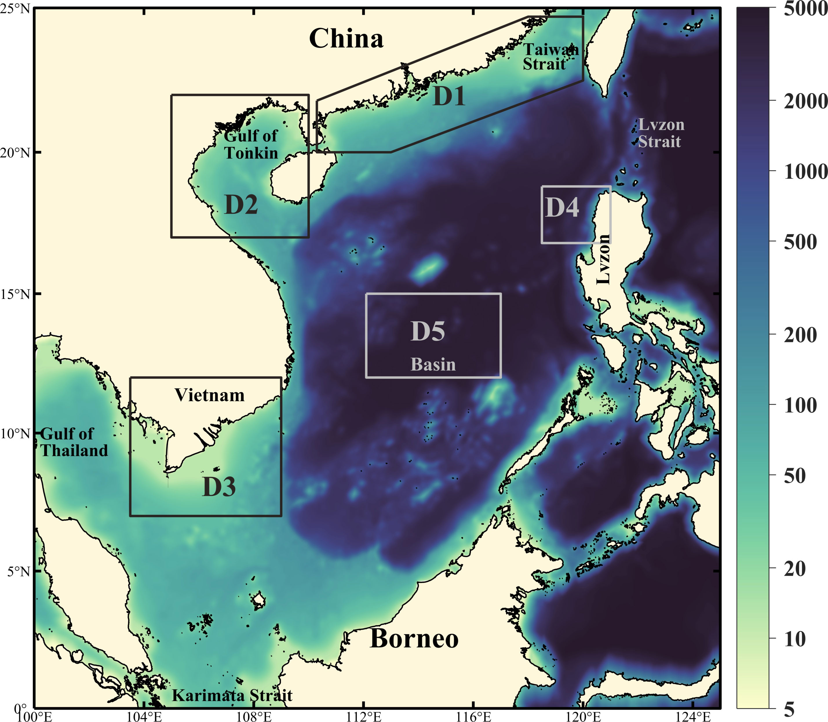
Figure 1 Bathymetry of the South China Sea model (unit: m). Five physical-biogeochemical domains are shown in the black/gray boxes (D1: the coast of China; D2: the Gulf of Tonkin; D3: the southern coast of Vietnam; D4: the west of Lvzon Island, and D5: the SCS basin).

Previous studies have shown great efforts in understanding the carbon cycle by studying CO₂ flux and its control factors through observations and numerical modeling (Marinov et al., 2008; Chen et al., 2013; Laruelle et al., 2017; Tian et al., 2019; Li et al., 2020; Li et al., 2020; McKinley et al., 2020; Wang et al., 2020; Ko et al., 2021). Li et al. (2020) summarized seasonal variations of oceanic surface pCO₂ and regional features of air-sea CO₂ fluxes over the SCS based on observations from 2000 to 2018. Chai et al. (2009) used a physical-biological coupled model with a 50km resolution and concluded that SST was a dominant factor in the seasonal variation of oceanic surface pCO₂, and the influence of biological activities was also significant over the SCS. However, due to the limits of time coverage and spatial resolution of the observations and numerical models, previous studies fail to present a detailed long-term variation trend of oceanic surface pCO₂, and uncertainties remain in understanding drivers of oceanic surface pCO₂ variations on seasonal and interannual time scales over the SCS. With complex geographical and environmental conditions in the SCS, a high-resolution numerical model can help reconstruct coastal and basin-scale physical and biogeochemical status to remedy the insufficient capability for observing long-term trends of essential variables that control oceanic surface pCO₂. The physical-biological processes are complex in this region, therefore, understanding the carbon cycle in the SCS makes a positive contribution to understanding the role of marginal seas in the global carbon system and its response to climate change.

The present study is organized as follows: datasets and model settings are introduced in Section 2; the seasonal and interannual variations of oceanic surface pCO₂ are described in Section 3; the long-term trend rate of oceanic surface pCO₂ and its controlling factors are analyzed and discussed in Section 4; and conclusions are presented in section 5.

2 Data and model

2.1 Data

We introduced four sets of data in this study for model validation and long-term trend analysis of oceanic surface pCO₂. These included two sets of quality-controlled in-situ observation datasets to examine the capability of faithfully capturing features of oceanic surface pCO₂ variations of the model.

The monthly oceanic pCO₂ satellite dataset with a spatial resolution of 1°×1° was obtained from the Japan Meteorological Agency (JMA, datasets are accessible from their website https://www.data.jma.go.jp/gmd/kaiyou/english/co2_flux/co2_flux_data_en.html). The oceanic pCO₂ field was calculated from satellite observations of SST, SSS, and surface chlorophyll-a concentration (Iida et al., 2020).

Monthly in-situ observations of ocean surface pCO₂ were obtained from the dataset of Global Ocean Surface Carbon, which was provided by the E.U. Copernicus Marine Service Information (DOI: 10.48670/moi-00047). The data were with a resolution of 1°×1°, and the time coverage used in this study was from January 1990 to December 2021 (Chau et al., 2022).

Monthly modeled ocean surface pCO₂ came from the Global Ocean Biogeochemistry Hindcast dataset obtained from the E.U. Copernicus Marine Service Information (DOI: 10.48670/moi-00019). The datasets were based on the PISCES biogeochemical model with a resolution of 0.25°×0.25°, whose time coverage was between 1 January 1993 and 31 December 2020.

Monthly in-situ observations of atmospheric CO₂ concentration from Mauna Loa Observatory (MLO) (19.5°N, 155.6°W) were obtained from the Scripps Institution of Oceanography (Scripps CO₂ Program) from 1990 to 2021 (Keeling et al., 2005).

2.2 Coupled physical-biogeochemical model settings

The physical model in this study was based on the Regional Ocean Model System (ROMS) v3.7 (svn trunk revision 874 released in 2017) (Shchepetkin and McWilliams, 2005). The model configuration follows Zhu et al. (2022) in the study of the comparison and validation of ocean forecasting systems over the SCS. The model domain in this study covers 0° to 25°N and 100° to 125°E (as displayed in Figure 1) with a horizontal resolution of 1/30°, and vertical levels of 50 in σ coordinate in the upper 300m for a more sufficient resolution to resolve the thermocline well. The land-sea grid was redistributed for a better fit to the complex SCS coastline. The bathymetry was derived from the General Bathymetric Chart of the Oceans (GEBCO) global continuous terrain model for ocean and land with a 30 arcsec spatial resolution. The atmospheric forcing uses the ERA5 reanalysis dataset that has higher resolution in both spatial and temporal resolutions, and the method adopts the COARE3.0 bulk algorithm (Fairall et al., 2003) to calculate the air-sea momentum. More details about the SCS physical model configuration and simulation ability are introduced by Zhu et al. (2022).

The Carbon, Silicate, and Nitrogen Ecosystem (CoSiNE) model was used for biogeochemical stimulation in this study. Fifteen state variables were considered: four nutrients (ammonium, nitrate, silicate, and phosphate), two phytoplankton groups (picophytoplankton and diatoms), two zooplankton groups (microzooplankton and mesozooplankton), two types of chlorophyll-a, two types of detritus for simulating sinking and suspending, dissolved oxygen, TALK, and TCO₂. In addition, light input was considered. All the abovementioned variables used in the CoSiNE model can affect the carbonate system, which is also affected by physical processes concurrently. More detailed settings can be found in Chai et al. (2002) and Xiu and Chai (2013).

To reach a climatologically steady state of circulation model, the physical circulation model was run for a 26-year climatology state before being coupled with the biogeochemical model, and then the CoSiNE model was coupled with the physical model on the same model grid. The time step was set as 5 seconds for the external mode and 150 seconds for the internal mode.

2.3 Determining control factors of oceanic surface pCO₂

Oceanic surface pCO₂ shows a distinct positive correlation with atmospheric CO₂ concentration when the influence of anthropogenic CO₂ is taken into consideration. In addition, the variation of oceanic surface pCO₂ is also related to changes in SST, SSS, TALK, and TCO₂ according to previous studies (Takahashi et al., 2002; McKinley et al., 2006; Takahashi et al., 2009; Ji et al., 2022). To further estimate drivers of the variation rate of oceanic surface pCO₂ on the interannual time scale, we used the formula as follows to linearize the change of oceanic surface pCO₂ (Takahashi et al., 1993; McKinley et al., 2006; Xiu and Chai, 2014; Ji et al., 2022):

$\begin{array}{ll}\Delta {\text{pCO}}_2=\frac{\partial {\text{pCO}}_2}{\partial \text{SST}}\times \Delta \text{SST}+\frac{\partial {\text{pCO}}_2}{\partial \text{SSS}}\times \Delta \text{SSS}+\frac{\partial {\text{pCO}}_2}{\partial {\text{TCO}}_2}\times \Delta {\text{TCO}}_2+\frac{\partial {\text{pCO}}_2}{\partial \text{TALK}}\times \Delta \text{TALK}& (1)\end{array}$

To isolate variables and evaluate the influence of each control factor on the $\Delta p{\text{CO}}_2$, while calculating $\Delta p{\text{CO}}_2$, only the interested one control variable changes and other variables were set to their long-term mean values on the right-hand side of the above equation.

3 Results

3.1 Model validation

The SCS model was examined and validated before further analysis. Three sets of monthly oceanic pCO₂ datasets were used to compare with the SCS model result, namely, the Global Ocean Biogeochemistry Hindcast (hereinafter referred to as CMEMS_Model), the Global Ocean Surface Carbon in-situ observations (hereinafter referred to as CMEMS_Obs), and the satellite observations from the Japan Meteorological Agency (hereinafter referred to as JMA_Satellite). According to the time coverage of datasets, the validation period was between 1993 and 2019.

The temporal variations of monthly mean oceanic surface pCO₂ anomaly at the SEATS station (18°N, 116°E) from January 1993 to December 2019 obtained from the SCS model, CMEMS model, CMEMS observation, and JMA satellite data were compared (Figure 2). All datasets showed increasing trends of the oceanic surface pCO₂ in the SCS. The standard deviations of the increasing rates of the SCS model and CMEMS model were both low with a value of 11.60, which indicates that the SCS model can ably reconstruct and simulate the oceanic surface pCO₂ (Table 1). Validation results showed that the SCS model fits well with the temporal patterns with a generally increasing trend over time. The SCS model appeared to be greater than the observations and CMESM model, which may be related to a stronger upwelling simulation performance of the physical model.

FIGURE 2

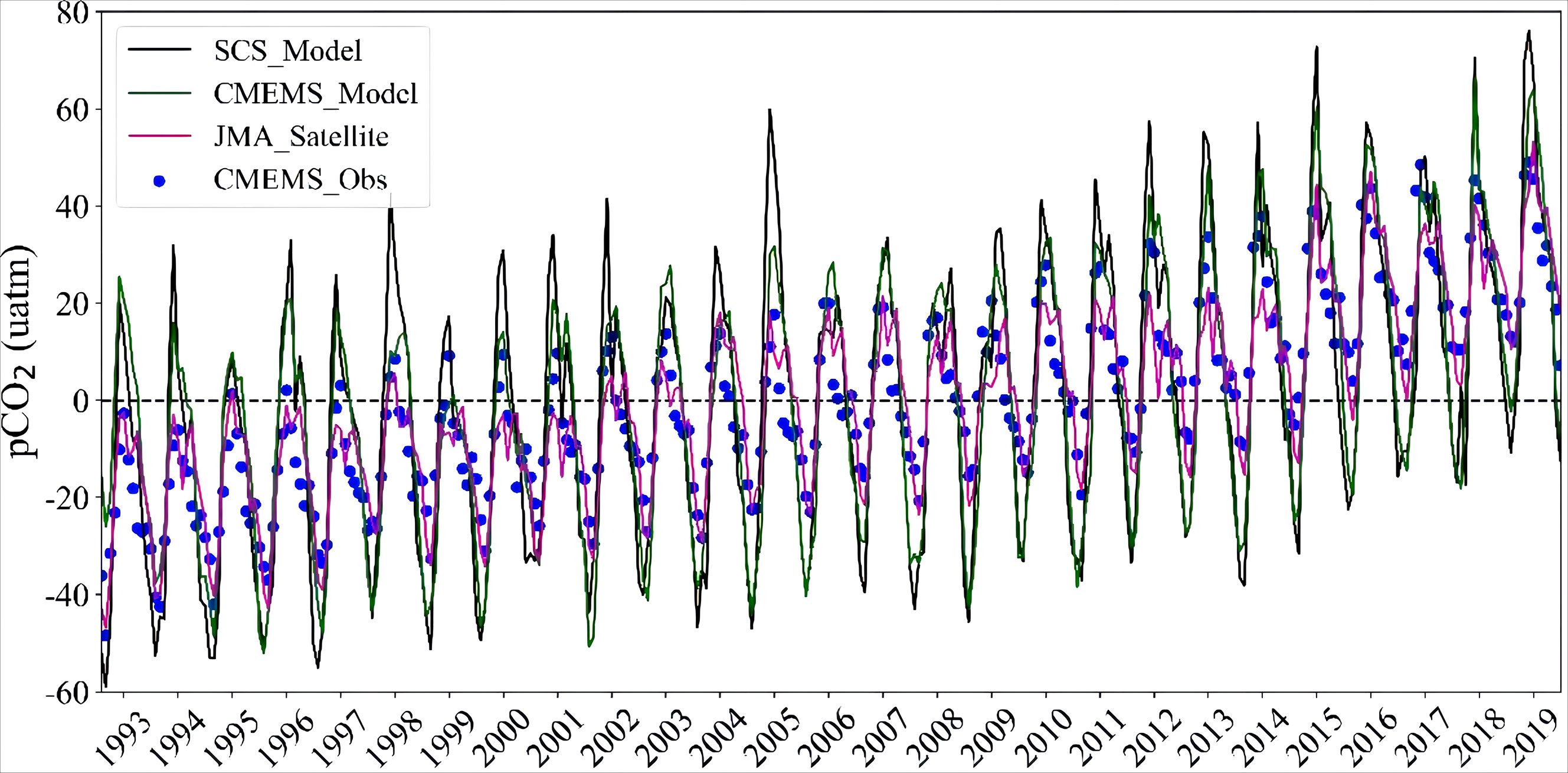
Figure 2 The temporal variations of the oceanic surface pCO₂ at SETAS from January 1993 to December 2019. The black line represents the SCS model output, the green line represents the CMESM model output, the blue dots represent CMESM in-situ observation, and the purple line represents the JMA satellite datasets, units: μatm.

TABLE 1

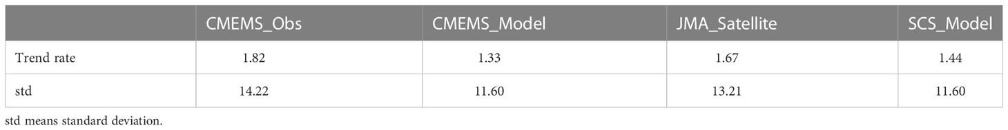
Table 1 The increasing rates of oceanic surface pCO₂ calculated with different datasets in the SCS from January 1993 to December 2019, units: μatm a^-1.

The spatial distributions of the climatological oceanic surface pCO₂ obtained from the datasets and the SCS model all showed strong regional characteristics that the pCO₂ level is higher in the south and lower in the north, especially along the continental shelf regions (Figure 3). High pCO₂ values appear in the estuary areas (i.e., the Pearl River estuary, Red River estuary, and Mekong River estuary) due to the input of river discharge that contains a large number of nutrients and dissolved inorganic carbon (DIC) (Figures 3C, D). Due to the differences in spatial resolution of datasets, SCS model outputs showed more detailed variations in the spatial distribution of climatological oceanic surface pCO₂. Factors that influence variation and changing rate of oceanic surface pCO₂ will be discussed in the following sections. In general, the SCS model can ably reproduce variations of oceanic surface pCO₂.

FIGURE 3

Figure 3 The spatial distribution of the climatological oceanic surface pCO₂ in the SCS from January 1993 to December 2019, units: μatm. (A) JMA satellite datasets; (B) CMEMS in-situ observation; (C) CMEMS model outputs; (D) SCS model result.

3.2 Seasonal variation of oceanic surface pCO₂

The spatial distributions of oceanic surface pCO₂ and surface chlorophyll concentration, the temporal variations of atmospheric pCO₂, oceanic surface pCO₂, SST, and surface chlorophyll concentration in the SCS will be analyzed in this section, as well as the climatological seasonal variations that were obtained from the SCS modeled monthly mean values from January 1992 to December 2021. In this study, four seasons were set as follows: spring (averaged from March-April-May), summer (averaged from June-July-August), autumn (averaged from September-October-November), and winter (averaged from December-January-February).

The modeled climatological oceanic surface pCO₂ showed strong seasonal variability and regional characteristics in terms of spatial distribution (Figure 4). The regions with pCO₂ value higher than 400 μatm gradually spans from concentrating in the Karimata Strait in winter to covering the entire SCS in summer.

FIGURE 4

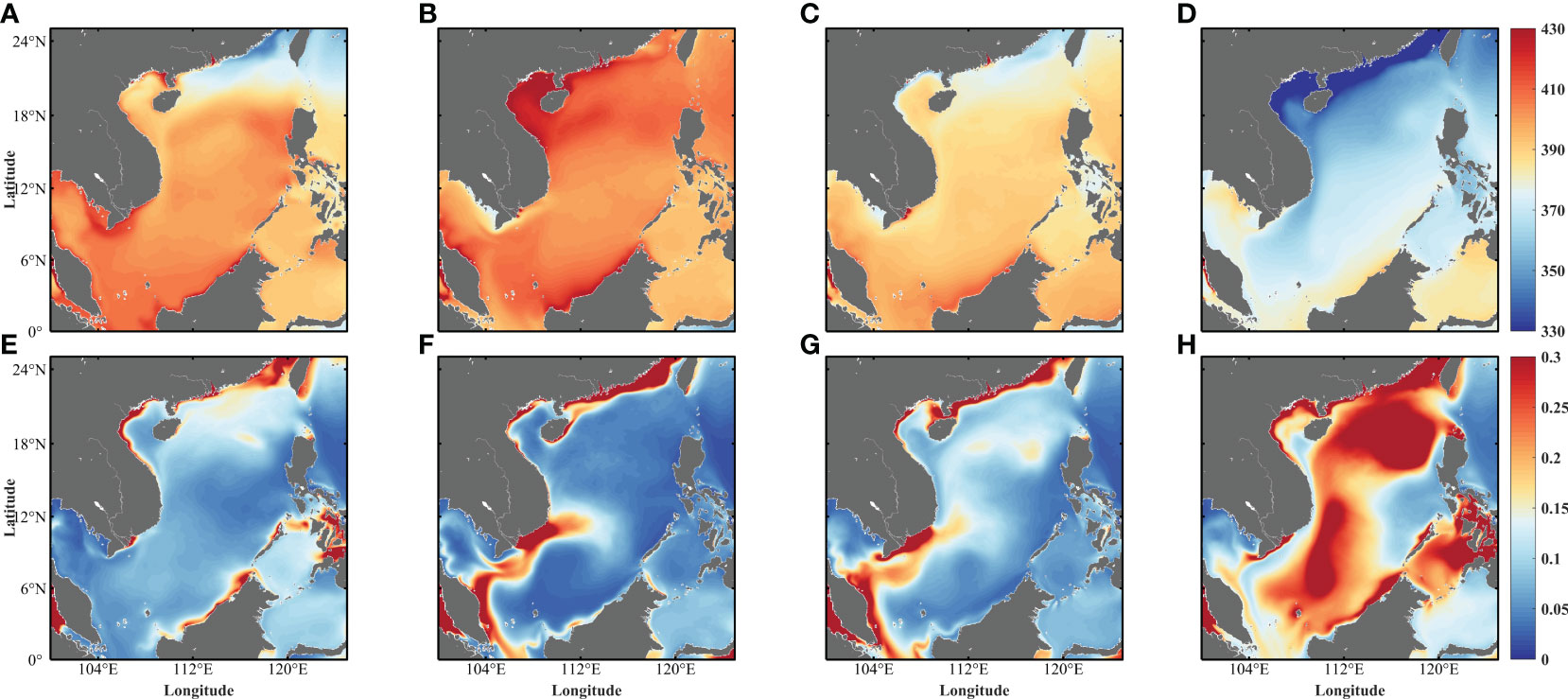
Figure 4 The spatial distributions of seasonal variations of the climatological oceanic surface pCO₂ (units: μatm, shown in upper panel) and chlorophyll concentration (units: mg·m^-3, shown in bottom panel). (A, E) spring, (B, F) summer, (C, G) autumn, and (D, H) winter.

The oceanic surface pCO₂ decreased with the latitude from 378 μatm near the west coast of Borneo to 332 μatm on the coast of China in winter. As the annual mean atmospheric pCO₂ was 381μatm, which is derived from the MLO observations, the SCS serves as a CO₂ sink in this season. The biological productivity was more active in winter than during the other three seasons as a result of lower SST and stronger mixing process (Figures 4E–H), which consumes a massive amount of TCO₂ in water and thus intensifies the decrease of pCO₂ in the surface water (Figure 4D).

The spatial mean oceanic pCO₂ showed a slight increase to 388 μatm in spring along with the rise of seawater temperature, which suggests the SCS, in general, turns into a weak source of CO₂ in this season (Figure 4A). However, along the coast of China, the oceanic pCO₂ level was relatively low with an average value of 365 μatm in the north of 20°N, and compared to the other parts, the CO₂ fluxes were from the air to the sea in this region.

In summer, the oceanic pCO₂ reached a domain-mean value of 400 μatm, and the maximum value of 425 μatm was spotted in the Gulf of Tonkin (Figure 4B). However, a relatively low value appeared near the southern coast of Vietnam with an oceanic pCO₂ level of 387 μatm, which was the result of the combined influence of monsoon-induced upwelling and biological productivity (Chai et al., 2009). Summer monsoon strengthens upwelling in such regions thus transporting cold water and nutrients to the surface, which enhances biological production near the coast of Vietnam; therefore, with the consumptions of TIC, the oceanic surface pCO₂ in this region appears to be lower than adjacent areas. Since the minimum value was still higher than atmospheric pCO₂, the entire SCS acts as a CO₂ source to the atmosphere in summer.

Similar to the distribution pattern in spring, the oceanic pCO₂ decreased with the increasing latitude in autumn, with an average value of 388 μatm (Figure 4C). The narrow west coast off of Borneo was with a higher value of 398 μatm; while in the northern shelf of the SCS, oceanic pCO₂ was relatively low at 377 μatm, an area that is the CO₂ sink of the SCS in autumn. Overall, the climatological oceanic surface pCO₂ spatial distribution showed strong seasonal disparity, and the regional distribution difference was in agreement with the findings by Chai et al. (2009). The mechanisms of variations of oceanic surface pCO₂ will be discussed in section 4.2.

In terms of the temporal variations of the associated oceanic surface variables, the domain-averaged climatological values of atmospheric pCO₂, oceanic pCO₂, SST, and chlorophyll-a concentration were compared and analyzed (Figure 5). The monthly mean oceanic pCO₂ varied between 357 and 408 μatm and peaked in June. After the peak, the decreasing rate of oceanic pCO₂ showed a slight inflection point in September (with a value of 395 μatm), with accelerated decreases afterward. The annual mean climatological atmospheric pCO₂ was around 381 μatm, indicating the SCS is a source of CO₂ into the atmosphere from March to October and a sink from November to February, which is in agreement with the findings by Wong et al. (2007). A resemblant pattern was detected in the temporal variation of SST, whose monthly mean varied between 25.6 and 29.4°C. The highest value occurred in June, followed by a slight inflection point in September (29.0°C). The seasonal cycles of SST and oceanic pCO₂ were closely linked, indicating seawater temperature positively correlates with the variation of oceanic pCO₂.

FIGURE 5

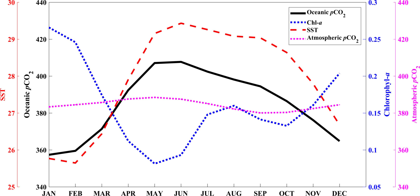
Figure 5 The seasonal cycles of climatological SST (units: °C, red dash line), oceanic surface pCO₂ (units: μatm, black solid line), chlorophyll-a concentration (units: mg·m^-3, blue dotted line), and atmospheric pCO₂ (units: μatm, magenta dotted line).

On the contrary, a reverse relationship between oceanic pCO₂ and chlorophyll-a concentration was observed. Monthly mean chlorophyll-a concentration varied between 0.08 and 0.27 mg m^-3, with a maximal value in January and a minimum value in May. The reason for the reverse patterns of chlorophyll-a concentration and oceanic pCO₂ is that the most active biological productivity exists in winter in the SCS, which benefits from enriched nutrients and DIC in the upper layer from the strong mixing process, therefore, more CO₂ is removed from the water by photosynthesis, thus decreasing the oceanic pCO₂; while in late spring to early summer, chlorophyll-a concentration drops to the bottom indicating the photosynthesis is limited by the nutrient supply. With less CO₂ being removed and higher SST, oceanic surface pCO₂ reaches the peak value in June. The modeled oceanic variable patterns were in agreement with previous studies (Liu et al., 2002; Cao et al., 2019).

The positive correlation between oceanic pCO₂ and SST and the negative correlation between oceanic pCO₂ and chlorophyll-a concentration suggest that the seasonal cycle of oceanic surface pCO₂ was decided by variations of SST and biological productivity in the SCS. Therefore, related variables (SST, TCO₂, TALK, and SSS) were isolated to further examine their individual effects on controlling oceanic surface pCO₂ variation, as will be discussed in section 4.

3.3 Interannual variation of oceanic surface pCO₂

Interannual and decadal variations of oceanic surface pCO₂ were examined using the Empirical Orthogonal Function (EOF) analysis. EOF analysis was first conducted on normalized oceanic surface pCO₂ without the linear trend being removed. Under such circumstances, the first EOF mode for oceanic surface pCO₂ explained 81.73% of the total variance with an increasing trend over the entire SCS (figure not shown). The correlation coefficient between the first principal component (PC1) and deseasonalized atmospheric CO₂ was 0.92, which indicates that the atmospheric CO₂ uptake significantly contributed to the increase of oceanic surface pCO₂ since the 1990s with an accelerating increase of anthropogenic CO₂ emissions. The correlation coefficients between the PC1 and normalized SST and TCO₂ were 0.69 and 0.74, respectively, which indicates tight links between oceanic pCO₂ and the abovementioned variables. The normalized oceanic surface pCO₂ and SST both showed significant increases from the year 1997 to 1998 and from 2015 to 2016, which may link with the extreme warming events in the SCS in the corresponding period (Xiao et al., 2017; Xiao et al., 2020).

As this mode explained over 80% of the total pCO₂ variance, the linear trend was removed to further examine correlations between oceanic surface pCO₂ and climatic indexes. Monthly modeled outputs from 1992 to 2021 were deseasonalized and detrended with the linear long-term trend, and the Niño 3 index and the PDO indices were introduced into the analyses to link with climate variability for a further understanding of interannual and decadal variations of oceanic surface pCO₂.

The first EOF mode of the detrended oceanic pCO₂ appeared to be positive over the entire region, especially in the Gulf of Tonkin and the central to the southern part of the SCS, which explains 44.17% of the total variance (Figure 6A). The minimum values were distributed along the northern coast of the SCS, especially around the Pearl River plumes, which is consistent with the findings by Li et al., 2020 and Wang et al. (2020). The PC1 showed a positive response to the Niño 3 index with a correlation coefficient of 0.51 with the Niño 3 leads 5 months, which indicates an interannual modulation of oceanic surface pCO₂ by SST, and a strong influence of ENSO on the carbonate system in the SCS. The second EOF mode explained 8.16% of the total variance and exhibited a clear north-south dipole distribution (Figure 6B). The PC2 after the three-point smooth was significantly correlated with the PDO index (R=0.62) with PDO leads 7 months, which indicates there is a strong influence of the PDO on the decadal variation of the oceanic pCO₂ in the SCS. The third EOF mode explained approximately 4.48% of the total variance showing a meridional structure centered around 114°E and it could possibly relate to a mixed modulation of climate variations that need to be further investigated (Figure 6C).

FIGURE 6

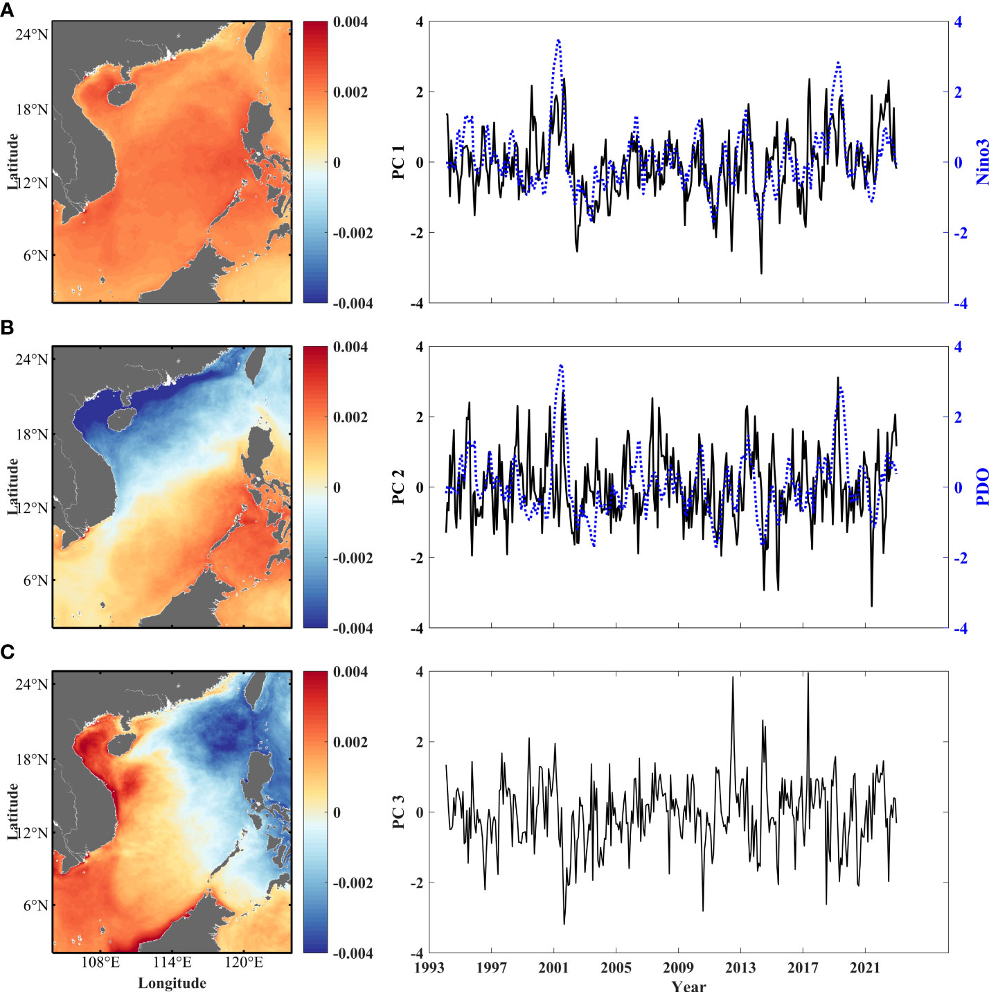
Figure 6 The three dominant EOF modes of the detrended oceanic surface pCO₂ (left panel) and their associated principal components (right panel). (A) EOF1 detrended and PC1 with the Niño3 index (5-month lag) superimposed on the PC1 mode (blue dotted line), (B) EOF2 detrended and PC2 with the PDO (7-month lag) superimposed on the PC2 mode (blue dotted line), (C) EOF3 detrended and PC3.

4 Discussion

4.1 The trend rate of oceanic surface pCO₂

In this section, long-term trend rates of oceanic surface variables (SST, TCO₂, TALK, and SSS) were calculated and analyzed to examine their correlations with the trend rate of oceanic surface pCO₂. Due to the strong regional disparity of the abovementioned variables, the SCS was separated into five domains based on physical-biogeochemical conditions and previous studies to further explore geographical features of the various rates (Yu et al., 2019; Li et al., 2020; Wang et al., 2020). The domains were (D1) the coast of China (21.8°~24.7°E, 110.3°~120°N), (D2) the Gulf of Tonkin (17°~22°E, 105°~110°N), (D3) the southern coast of Vietnam (7°~12°E, 103.5°~109°N), (D4) the west of Lvzon Island (16.8°~18.8°E, 118.5°~121°N), and (D5) the SCS basin (12°~15°E, 112.1°~117°N). Detailed physical-biogeochemical descriptions of domains are displayed in Table 2 The water channels and confluent areas of large runoffs (here it refers to regions around the Pearl River estuary, the Red River estuary, and the Mekong River estuary) were removed from calculation to diminish the impact of runoff when examining the oceanic surface variables. The range of influence of SSS variation was limited around the estuary zone and did not show any significant regional changing trend (average value was less than 0.01 psu/a), therefore its spatial distribution is not shown in Figure 7.

TABLE 2

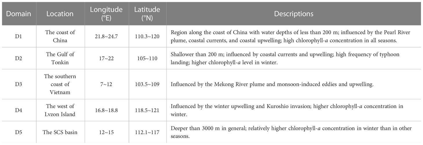
Table 2 Summary of the five physical-biogeochemical domains in the SCS.

FIGURE 7

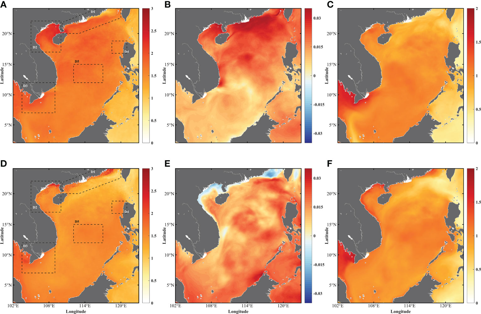
Figure 7 The spatial distributions of the long-term trend rates of the change of oceanic surface variables in summer (upper panel) and in winter (bottom panel). (A, D) oceanic surface pCO₂ change rate distribution, units: μatm·a^-1; (B, E) SST change rate distribution, units: °·a^-1; (C, F) TCO₂ change rate distribution, units: mmol·m^-3·a^-1. The five physical-biogeochemical domains are shown in black dotted boxes in (A).

Since oceanic surface pCO₂ was mainly decided by variations of SST and biological productivity, the trend rate of oceanic pCO₂ was controlled by the balance of water temperature change, upwelling and removing of TCO₂, and TALK concentration variation. Besides seasonal variations of net heat flux, carbon cycle, seawater temperature, and accompanied chlorophyll-a concentration variations were also associated with the coastal currents and upwelling physics in the SCS, meaning the East Asian Monsoon plays a vital role in regulating the variation of oceanic pCO₂ in this region in summer and winter (Hu et al., 2003; Xie et al., 2003; Anderson et al., 2009; Liu et al., 2010).

The modeled oceanic pCO₂, SST, and TCO₂ over the entire SCS all showed positive long-term rates of change with a domain-averaged value of 1.19 ± 0.60 μatm/a for oceanic pCO₂, 0.018 ± 0.004°C/a for SST, and 0.62 ± 0.34 mmol·m^-3/a for TCO₂, which were all under the influences of global warming and the increase of anthropogenic CO₂ emissions in the latest decades. A positive long-term trend rate of TALK was also observed (figure not shown); with the neglection of river discharge in this study, the TALK variation was mainly regulated by ocean currents (Yang and Byrne, 2022).

D1 and D2 are typical shelf marine systems and share common seasonal variations along the shorelines from the Taiwan Strait to the Gulf of Tonkin. The modeled SST trend rate was high in summer and low in winter in both regions (Figures 7B, E; Table 3) with a peak value among all five regions of 0.029 ± 0.005°C/a in summer in D1, and a runner-up value of 0.021 ± 0.006°C/a appearing in D2, which is in agreement with the findings by Yu et al. (2019). The warming trend leads to an intensification of stratification of the water column, therefore inhibiting the increase of TCO₂ in return, so the trend rate of TCO₂ was lower in summer than in winter in both regions (Figures 7C, F; Table 3). Under the combined influences of a strong warming trend of SST and a weak increasing trend of TCO₂, the oceanic surface pCO₂ trend rates were much higher in summer than in winter in both regions, the differences between the two seasons were 0.35 μatm/a and 0.43 μatm/a, respectively (Figures 7A, D; Table 3). Therefore, in the shelf system, SST makes a greater contribution to the increase of oceanic surface pCO₂ in summer, and TCO₂ accounts for a positive trend in both seasons.

TABLE 3

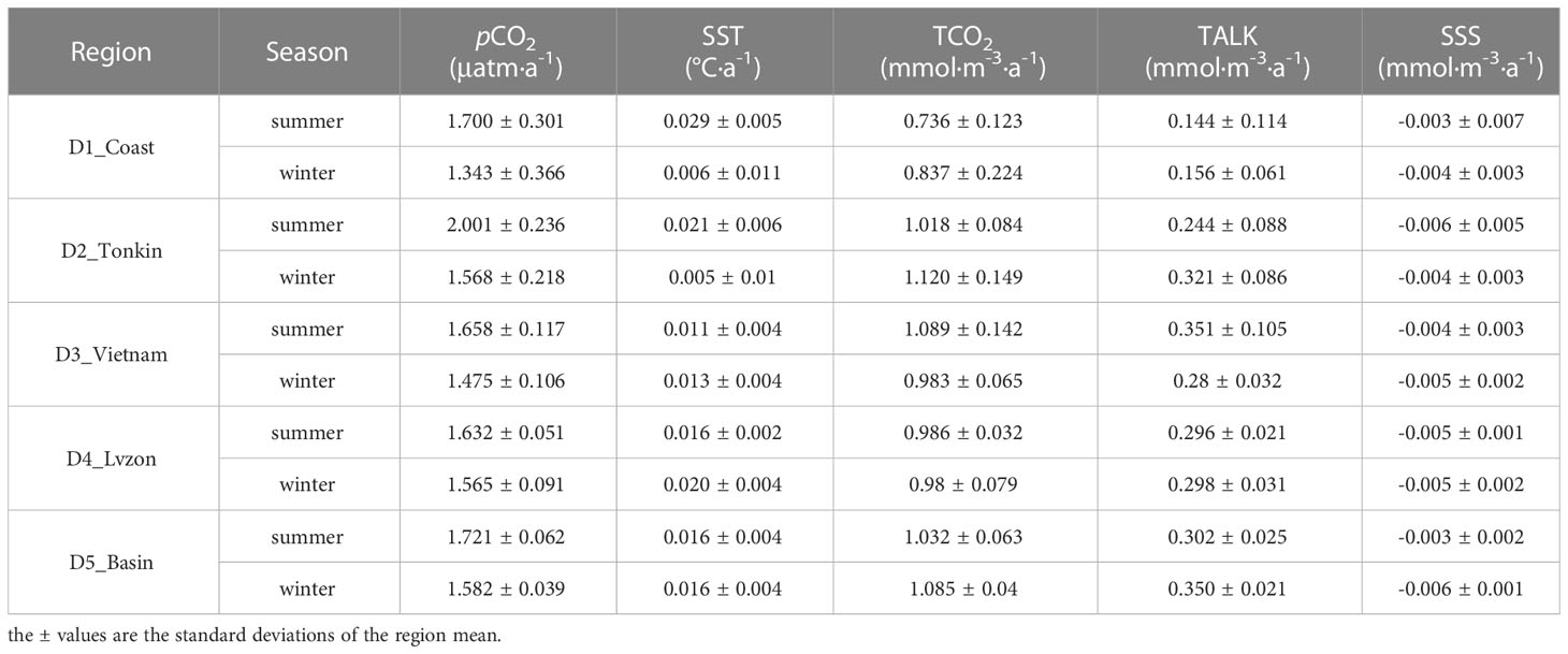
Table 3 Long-term trend rates of oceanic surface pCO₂, SST, TCO₂, and TALK in summer and winter in the five physical-biogeochemical domains.

In D3, owing to the prevailing monsoon system over the SCS, oceanic variables showed pronounced seasonality. In summer, the southwesterly monsoon strengthened the upwelling near the shoreline, and the increasing trend of TCO₂ and TALK were both observed in summer in this region (Table 3), which is under the influence of monsoon-induced upwelling that brings cold water, TCO₂, and nutrients in the subsurface layer up to the upper layer (Xie et al., 2003; Jing et al., 2016). Whereas, the modeled SST exhibited a “cold gyre” showing a slightly decreasing trend (Figure 7B), which may be related to the Vietnam cold eddies induced by monsoon and land topography (Yuan et al., 2005; Hu et al., 2011; Valsala and Murtugudde, 2015). In winter, with the prevailing wind turning northeasterly, upwelling along the Vietnam coast was weakened, which brought a relatively warmer trend of SST in the extended area (Table 3). With the inhibiting effect of high SST and consumption from biological production and remineralization, TCO₂ and TALK as a result showed weak increasing rates (Figure 4H; Table 3). The oceanic pCO₂ maintained a high increasing trend rate in the summer and low in the winter, which suggests it is dominated by the variation of TCO₂ (this will be further illustrated in section 4.2).

The northeasterly monsoon wind promoted upwelling effects in D4 and D5 in winter; nutrients and TCO₂ were transported to the upper layer, which contributed to the increase in the trend rate of TCO₂ (Chen et al., 2022). In addition, the intrusion of the Kuroshio current in the SCS peaks from the fall to January, which contributes to a higher increasing rate of SST from Lvzon Strait to the west of the SCS in winter (Xue et al., 2004; Nan et al., 2015). However, the trend rate of TCO₂ around the west off Lvzon Island (D4) was lower in winter even with the positive influence of monsoon-induced upwelling (Table 3), and the reason is that the biological productivity is significant (the average value of chlorophyll-a concentration is over 0.3 mg/m³), and it balances out the positive effect of upwelling, resulting in a weakened TCO₂ increase in winter; while the promoting effect of monsoon-induced upwelling gradually recedes in summer, which benefits the increasing trend of TCO₂ due to the weakened biological productivity in D4. The long-term trend rates of oceanic variables were relatively stable in D5 as an abysmal region (Table 3).

Overall, among the five typical regions, the trend rate of oceanic surface pCO₂ was mainly controlled by the balance between SST variations, and input and removal of TCO₂. Therefore, control factors for long-term oceanic surface pCO₂ trend rate will be discussed through influence factor decomposition in the next section by focusing on the effects of SST and TCO₂ from region to region.

4.2 Drivers for long-term oceanic surface pCO₂ trends in different regions

Control factors including SST, TCO₂, TALK, and SSS were examined to determine the critical factor influencing the long-term trend rate of oceanic surface pCO₂ following Equation (1). The contributions from each variable were analyzed, and negative values of pCO₂-TALK and pCO₂-SSS were detected in most of the regions (Table 4). The effects of pCO₂-TALK and pCO₂-SSS were mainly the reflections of precipitation, evaporation, riverine inputs, and biological removal (Huang et al., 2015; Huang et al., 2021). By comparing to influences of pCO₂-SST and pCO₂-TCO₂, their contributions to the change rate of oceanic pCO₂ were insignificant (Xiu and Chai, 2014; Sutton et al., 2017), therefore only drivers of pCO₂-SST and pCO₂-TCO₂ in summer and winter are shown in Figure 8.

TABLE 4

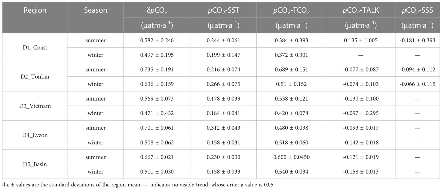
Table 4 Long-term trend rates of pCO₂ under influences of SST, TCO₂, TALK, and SSS in summer and winter in the five physical-biogeochemical domains.

FIGURE 8

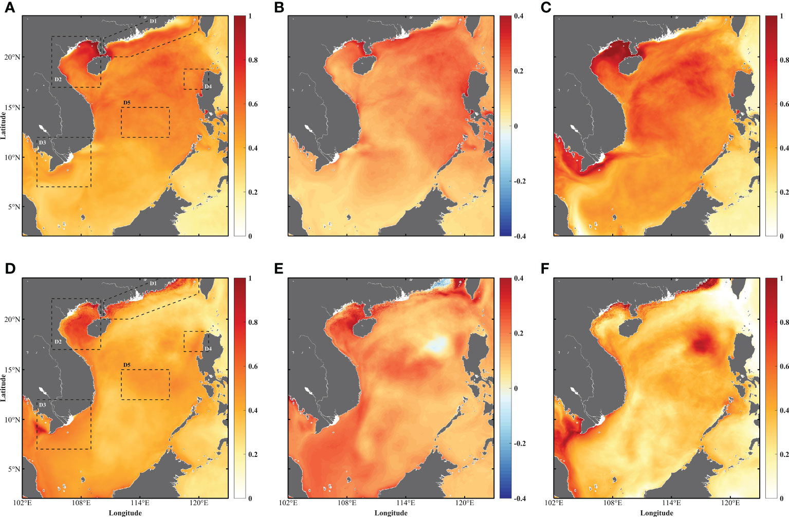
Figure 8 The spatial distributions of the long-term trend rates of change of pCO₂ in summer (upper panel) and in winter (lower panel), units: μatm·a^-1. (A, D) pCO₂; (B, E) pCO₂-SST; (C, F) pCO₂-TCO₂. The five physical-biogeochemical domains are shown in black dotted boxes.

δpCO₂ showed an increasing trend in the SCS with a domain-average value of 0.54 μatm/a in summer and 0.45 μatm/a in winter. The δpCO₂ had a higher increasing rate in the north to the central SCS in summer; while in winter, the high trend value was mainly distributed in the shallow waters along the shorelines of China (Figures 8A, D). All five domains showed higher values of δpCO₂ in summer than in winter, which corresponded to the long-term trend rate of pCO₂. The trend of δpCO₂ in the Gulf of Tonkin achieved the maximum value within the five domains with values of 0.735 ± 0.191 μatm/a in summer and 0.636 ± 0.159 μatm/a in winter, which indicates that the ocean releases more CO₂ to the air in this region.

The contribution of SST to the trend rate of oceanic pCO₂ was consistent with the trend rate of SST in most regions, whose influence on the trend rate of oceanic pCO₂ was 33.85% in summer and 34.86% in winter. The positive trend rate of pCO₂-SST covered most of the regions in both seasons (Figures 8B, E), and negative trend rates were seen in the Taiwan Strait and around the west of Lvzon Island in winter, which indicates a decreasing trend of oceanic pCO₂ due to the reduction of SST trend rates (Figures 7E, 8E). The contribution of TCO₂ dominated the SCS in both seasons, whose influence on the trend rate of oceanic pCO₂ was 83.67% in summer and 87.93% in winter, indicating that TCO₂ is the major driver for the long-term trend of oceanic surface pCO₂ (Figures 8C, F).

In D1, the correlation coefficient between the trend rate of oceanic pCO₂ and the trend rate of pCO₂-SST was 0.23 in summer and 0.20 in winter, while the correlation coefficient between the trend rate of pCO₂ and the trend rate of pCO₂-TCO₂ was 0.46 in summer (accounting for 65.98% of oceanic pCO₂) and 0.86 in winter (accounting for 74.85% of oceanic pCO₂). Hence, the trend rate of pCO₂-TCO₂ was more decisive than the trend rate of pCO₂-SST in the shelf marine system, where the trend rate of oceanic pCO₂ was mainly influenced by coastal currents and coastal upwelling effects.

The domain D2 was with the largest trend rate value of oceanic pCO₂ in the five domains with a value of 0.735 ± 0.191 μatm/a, and the trend rate of pCO₂-TCO₂ accounted for 0.689 ± 0.151 μatm/a, suggesting its predominant function. On the other hand, the influence of SST was low in summer, which only accounted for 29.39% of the trend rate of oceanic pCO₂ (Table 4). The possible mechanisms are not certain yet, one possible cause may link with a high frequency of typhoon landing in this region in summer, with strong wind stress, heavy rainfall, intensified mixing effects, and accelerated air-sea exchange (Potter et al., 2017; Ko et al., 2021), hence resulting in a low contribution of pCO₂-SST and a high contribution of pCO₂-TCO₂. Further analysis and investigation are required on this subject in the future.

In D3, the seasonal variations of the trend rate of pCO₂-SST and pCO₂-TCO₂ were dominated by the East Asian Monsoon and had similar seasonal patterns as the variations of the trend rates of SST and TCO₂. The pCO₂-TCO₂ accounted for 94.55% of the trend rate of oceanic pCO₂ in summer and 89.17% in winter, indicating the predominance of TCO₂ in controlling the long-term trend rate of pCO₂ (Table 4).

The influence of TCO₂ in D4 and D5 was significant in winter, pCO₂-TCO₂ accounted for 101.97% in D4 and 105.68% in D5, as a result of the strong positive impact of monsoon-induced upwelling on TCO₂ (Table 4). Gyre structures distributed in the west of Lvzon Island were spotted (Figures 8E, F), which indicates abnormal values appeared for the trend rate of pCO₂-SST and pCO₂-TCO₂ in winter. This may correspond to mesoscale eddies or anomalous wind stress curl over the region (Guo et al., 2015; Xiao et al., 2019), and it is worth further analyzing the relationships between oceanic surface pCO₂ and mesoscale structures in future research work.

5 Conclusion

This study simulates oceanic surface pCO₂ in the SCS based on a three-dimensional physical-biogeochemical model for a better understanding of the seasonal and interannual variations of oceanic surface pCO₂, and drivers that regulate the variations in this region. Based on the results from the SCS model between 1992 and 2021, a stable increasing trend of oceanic surface pCO₂ was detected over the entire SCS, and the trend was tightly linked with global warming and the increase of atmospheric CO₂ emissions. The temporal variation of climatological oceanic surface pCO₂ varied between 357 and 408 μatm, and results showed that the SCS serves as a source of CO₂ from March to October, and a sink of CO₂ during the rest of the year. The oceanic surface pCO₂ showed a positive correlation with SST and TCO₂ and a negative correlation with chlorophyll-a concentration. On the interannual time scale, the Niño 3 index and the PDO index correlated with the first and second principal components of the detrended oceanic pCO₂, which indicates the influences of ENSO and other climate variations on the oceanic pCO₂ variation.

The trend rate of oceanic surface pCO₂ was mainly affected by SST variations and input and removal of TCO₂. In the shelf system (D1 and D2), the variation of oceanic pCO₂ was more strongly correlated with SST (especially in the summer) as a result of a stronger warming trend of SST and a weaker increasing trend of TCO₂ in summer, and TCO₂ was positively correlated with oceanic pCO₂ variation in both summer and winter. In areas dominated by the East Asian monsoon (D3, D4, and D5), the monsoon-induced upwelling promoted the increase of TCO₂ in the surface water, and the change of the trend rate of oceanic pCO₂ was mainly controlled by the input and removal of TCO₂.

The positive trend rate of δpCO₂ was detected in the whole region with a higher value in summer and a lower value in winter. It was found that TCO₂ and SST both contribute positively to the increase of the trend rate of δpCO₂, while TALK and SSS show negative contributions in most domains through the influence factor decomposition. The influence of TCO₂ on δpCO₂ was significantly greater than that of SST in all domains, which indicates that TCO₂ is the major driver for the variation of the long-term trend rate of oceanic surface pCO₂.

The seasonal and interannual variations of oceanic surface pCO₂ and drivers that regulate the variations were analyzed. The analyses showed that the oceanic pCO₂ is mainly controlled by TCO₂ on the seasonal scale and responds to ENSO and other climate variability on the interannual scale. Furthermore, the atmospheric CO₂ uptake makes a significant contribution to the increase of oceanic pCO₂ on decadal timescales, therefore understanding the carbon cycle in the SCS helps to better explain the role of marginal seas in the global carbon system in the age of climate change. With more uncertainties that climate change brings, the carbonate system in the SCS may continue to change, and it is worthy of further investigation and research.

Data availability statement

The raw data supporting the conclusions of this article will be made available by the authors, without undue reservation.

Author contributions

MZ analyzed the data and wrote the original draft. XZ performed the physical model and free-run simulations. XJ designed the study and helped with reading over and polishing the paper. AZ and JZ contributed to the manuscript. All authors approved the submitted version.

Funding

The research was supported by the project of Southern MarineScience and Engineering Guangdong Laboratory (Zhuhai) (nos.SML2020SP008), the National Key R&D Program of China(2022YFC3105102), and the National Natural Science Foundationof China (nos. 42176029).

Acknowledgments

This work has benefited from open access to numerous datasets provided by the E.U. Copernicus Marine Service Information, including monthly global ocean surface carbon observations (Available at: https://data.marine.copernicus.eu/product/GLOBAL_MULTIYEAR_BGC_001_029/description) and model outputs of global Biogeochemistry hindcast (Available at: https://data.marine.copernicus.eu/product/GLOBAL_MULTIYEAR_BGC_001_029/description). The monthly oceanic pCO₂ grided satellite observation was obtained from the Japan Meteorological Agency (JMA Ocean CO₂ Map) and is available at: https://www.data.jma.go.jp/gmd/kaiyou/english/co2_flux/co2_flux_data_en.html. The monthly atmospheric CO₂ concentration in-situ observation was obtained from the Scripps Institution of Oceanography (Scripps CO₂ Program) and is available at: https://scrippsco2.ucsd.edu/data/atmospheric_co2/mlo.html.

Conflict of interest

The authors declare that the research was conducted in the absence of any commercial or financial relationships that could be construed as a potential conflict of interest.

Publisher’s note

All claims expressed in this article are solely those of the authors and do not necessarily represent those of their affiliated organizations, or those of the publisher, the editors and the reviewers. Any product that may be evaluated in this article, or claim that may be made by its manufacturer, is not guaranteed or endorsed by the publisher.

References

Anderson R. F., Ali S., Bradtmiller L. I., Nielsen S. H. H., Fleisher M. Q., Anderson B. E., et al. (2009). Wind-Driven Upwelling in the Southern Ocean and the Deglacial Rise in Atmospheric CO2. Science (New York, N.Y. ) 323, 1443–1448. doi: 10.1126/science.1167441

PubMed Abstract | CrossRef Full Text | Google Scholar

Cai W.-J., Dai M., Wang Y. (2006). Air-sea exchange of carbon dioxide in ocean margins: a province-based synthesis. Geophys. Res. Lett. 33. doi: 10.1029/2006GL026219

PubMed Abstract | CrossRef Full Text | Google Scholar

Cai W.-J., Dai M., Wang Y., Zhai W., Huang T., Chen S., et al. (2004). The biogeochemistry of inorganic carbon and nutrients in the pearl river estuary and the adjacent northern south China Sea. Continental Shelf Res. 24, 1301–1319. doi: 10.1016/j.csr.2004.04.005

CrossRef Full Text | Google Scholar

Cao Z., Yang W., Zhao Y., Guo X., Yin Z., Chuanjun D., et al. (2019). Diagnosis of CO2 dynamics and fluxes in global coastal oceans. Natl. Sci. Rev. 7, 786–797. doi: 10.1093/nsr/nwz105

PubMed Abstract | CrossRef Full Text | Google Scholar

Chai F., Dugdale R., Peng T. H., Wilkerson F., Barber R. (2002). One-dimensional ecosystem model of the equatorial pacific upwelling system. part I: model development and silicon and nitrogen cycle. Deep Sea Res. Part II: Top. Stud. Oceanog. 49, 2713–2745. doi: 10.1016/S0967-0645(02)00055-3

CrossRef Full Text | Google Scholar

Chai F., Liu G., Xue H., Shi L., Chao Y., Tseng C.-M., et al. (2009). Seasonal and interannual variability of carbon cycle in south China Sea: a three-dimensional physical-biogeochemical modeling study. J. Oceanog. 65, 703–720. doi: 10.1007/s10872-009-0061-5

CrossRef Full Text | Google Scholar

Chao S.-Y., Shaw P.-T., Wu S. Y. (1996). Deep water ventilation in the south China Sea. Deep Sea Res. Part I: OceanograpH. Res. Pap. 43, 445–466. doi: 10.1016/0967-0637(96)00025-8

CrossRef Full Text | Google Scholar

Chau T. T. T., Gehlen M., Chevallier F. (2022). A seamless ensemble-based reconstruction of surface ocean pCO2 and air–sea CO2 fluxes over the global coastal and open oceans. Biogeosciences 19, 1087–1109. doi: 10.5194/bg-19-1087-2022

CrossRef Full Text | Google Scholar

Chen C. T. A., Huang T. H., Chen Y. C., Bai Y., He X., Kang Y. (2013). Air–sea exchanges of CO2 in the world’s coastal seas. Biogeosciences 10, 6509–6544.10.5194/bg-10-6509-2013. doi: 10.5194/bg-10-6509-2013

CrossRef Full Text | Google Scholar

Chen M., Zhao X., Li D.-W., Dong L. (2022). Mesoscale Eddy Effects on Nitrogen Cycles in the Northern South China Sea Since the Last Glacial. Front. Earth Sci. doi: 10.10.3389/feart.2022.886200

CrossRef Full Text | Google Scholar

Dore J. E., Lukas R., Sadler D. W., Church M. J., Karl D. M. (2009). Physical and biogeochemical modulation of ocean acidification in the central north pacific. Proc. Natl. Acad. Sci. USA 106, 12235–12240. doi: 10.1073/pnas.0906044106

CrossRef Full Text | Google Scholar

Fairall C. W., Bradley E. F., Hare J. E., Grachev A. A., Edson J. B. (2003). Bulk parameterization of air–Sea fluxes: updates and verification for the COARE algorithm. J. J. Climate 16, 571–591. doi: 10.1175/1520-0442(2003)016<0571:Bpoasf>2.0.Co;2

CrossRef Full Text | Google Scholar

Friedlingstein P., Jones M. W., O’Sullivan M., Andrew R. M., Bakker D. C. E., Hauck J., et al. (2022). Global carbon budget 2021. Earth Syst. Sci. Data 14, 1917–2005. doi: 10.5194/essd-14-1917-2022

CrossRef Full Text | Google Scholar

GEBCO GEBCO_2014 grid [data set]. Available at: https://www.gebco.net/data_and_products/historical_data_sets/#gebco_2014 (Accessed 12 December 2022).

Google Scholar

Guo M., Chai F., Xiu P., Li S., Rao S. (2015). Impacts of mesoscale eddies in the south China Sea on biogeochemical cycles. Ocean Dynam. 65, 1335–1352. doi: 10.1007/s10236-015-0867-1

CrossRef Full Text | Google Scholar

He Y., Cai S., Wang D., He J. (2015). A model study of Luzon cold eddies in the northern south China Sea. Deep Sea Res. Part I: OceanograpH. Res. Pap. 97, 107–123. doi: 10.1016/j.dsr.2014.12.007

CrossRef Full Text | Google Scholar

Hu J., Gan J., Sun Z., Zhu J., Dai M. (2011). Observed three-dimensional structure of a cold eddy in the southwestern south China Sea. J. Geophys. Res. 116. doi: 10.1029/2010jc006810

CrossRef Full Text | Google Scholar

Hu J., Kawamura H., Hong H., Qi Y. (2000). A review on the currents in the south China Sea: seasonal circulation, south China Sea warm current and kuroshio intrusion. J. Oceanog. 56, 607–624. doi: 10.1023/A:1011117531252

CrossRef Full Text | Google Scholar

Hu J. Y., Kawamura H., Tang D. L. (2003). Tidal front around the hainan island, northwest of the south China Sea. J. Geophys. Res. Oceans 108, 3342. doi: 10.1029/2003jc001883

CrossRef Full Text | Google Scholar

Huang W.-J., Cai W.-J., Hu X. (2021). Seasonal mixing and biological controls of the carbonate system in a river-dominated continental shelf subject to eutrophication and hypoxia in the northern gulf of Mexico. Front. Mar. Sci. 8. doi: 10.3389/fmars.2021.621243

CrossRef Full Text | Google Scholar

Huang W. J., Cai W. J., Wang Y., Lohrenz S. E., Murrell M. C. (2015). The carbon dioxide system on the Mississippi river-dominated continental shelf in the northern gulf of Mexico: 1. distribution and air-sea CO(2) flux. J. Geophys Res. Ocean. 120, 1429–1445. doi: 10.1002/2014JC010498

CrossRef Full Text | Google Scholar

Iida Y., Takatani Y., Kojima A., Ishii M. (2021). Global trends of ocean CO2 sink and ocean acidification: an observation-based reconstruction of surface ocean inorganic carbon variables. J. Oceanog. 77, 323–358. doi: 10.1007/s10872-020-00571-5

CrossRef Full Text | Google Scholar

Ji X., Chai F., Xiu P., Liu G. (2022). Long-term trend of oceanic surface carbon in the Northwest pacific from 1958 to 2017. Acta Oceanol. Sin. 41, 90–98. doi: 10.1007/s13131-021-1953-5

CrossRef Full Text | Google Scholar

Jing Z., Qi Y., Fox-Kemper B., Du Y., Lian S. (2016). Seasonal thermal fronts on the northern south China Sea shelf: satellite measurements and three repeated field surveys. J. Geophys. Res.: Ocean. 121, 1914–1930. doi: 10.1002/2015JC011222

CrossRef Full Text | Google Scholar

Keeling C. D., Piper S. C., Bacastow R. B., Wahlen M., Whorf T. P., Heimann M., et al. (2005). “Atmospheric CO2 and 13CO2 exchange with the terrestrial biosphere and oceans from 1978 to 2000: observations and carbon cycle implications,” in A history of atmospheric CO2 and its effects on plants, animals, and ecosystems. Eds. Baldwin I. T., Caldwell M. M., Heldmaier G., Jackson R. B., Lange O. L., Mooney H. A., et al (New York, NY: Springer New York).

Google Scholar

Ko Y. H., Park G.-H., Kim D., Kim T.-W. (2021). Variations in seawater pCO2 associated with vertical mixing during tropical cyclone season in the northwestern subtropical pacific ocean. Front. Mar. Sci. 8. doi: 10.3389/fmars.2021.679314

CrossRef Full Text | Google Scholar

Laruelle G. G., Landschützer P., Gruber N., Tison J.-L., Delille B., Regnier P. (2017). Global high-resolution monthly pCO2 climatology for the coastal ocean derived from neural network interpolation. Biogeosciences 14, 4545–4561.10.5194/bg-14-4545-2017. doi: 10.5194/bg-14-4545-2017

CrossRef Full Text | Google Scholar

Li Q., Guo X., Zhai W., Xu Y., Dai M. (2020). Partial pressure of CO2 and air-sea CO2 fluxes in the south China Sea: synthesis of an 18-year dataset. Prog. Oceanog. 182, 102272. doi: 10.1016/j.pocean.2020.102272

CrossRef Full Text | Google Scholar

Liu K. K., Chao S. Y., Shaw P. T., Gong G. C., Chen C. C., Tang T. Y. (2002). Monsoon-forced chlorophyll distribution and primary production in the south China Sea: observations and a numerical study. Deep Sea Res. Part I: OceanograpH. Res. Pap. 49, 1387–1412. doi: 10.1016/S0967-0637(02)00035-3

CrossRef Full Text | Google Scholar

Liu S. M., Guo X., Chen Q., Zhang J., Bi Y. F., Luo X., et al. (2010). Nutrient dynamics in the winter thermohaline frontal zone of the northern shelf region of the south China Sea. J. Geophys. Res. 115, C11020. doi: 10.1029/2009jc005951

CrossRef Full Text | Google Scholar

Marinov I., Gnanadesikan A., Sarmiento J. L., Toggweiler J. R., Follows M., Mignone B. K. (2008). Impact of oceanic circulation on biological carbon storage in the ocean and atmosphericpCO2. Global Biogeochem. Cycles 22, n/a–n/a. doi: 10.1029/2007gb002958

CrossRef Full Text | Google Scholar

McKinley G., Fay A., Eddebbar Y., Gloege L., Lovenduski N. (2020). External forcing explains recent decadal variability of the ocean carbon sink. AGU Adv. 1, e2019AV000149. doi: 10.1029/2019AV000149

CrossRef Full Text | Google Scholar

McKinley G. A., Takahashi T., Buitenhuis E., Chai F., Christian J. R., Doney S. C., et al. (2006). North pacific carbon cycle response to climate variability on seasonal to decadal timescales. J. Geophys. Res. 111, C07S06. doi: 10.1029/2005jc003173

CrossRef Full Text | Google Scholar

Nan F., Xue H., Yu F. (2015). Kuroshio intrusion into the south China Sea: a review. Prog. Oceanog. 137, 314–333. doi: 10.1016/j.pocean.2014.05.012

CrossRef Full Text | Google Scholar

Potter H., Drennan W. M., Graber H. C. (2017). Upper ocean cooling and air-sea fluxes under typhoons: a case study. J. Geophys. Res. Oceans 122, 7237–7252. doi: 10.1002/2017JC012954

CrossRef Full Text | Google Scholar

Shchepetkin A. F., McWilliams J. C. J. O. M. (2005). The regional oceanic modeling system (ROMS): a split-explicit, free-surface, topography-following-coordinate oceanic model. Ocean Modelling 9, 347–404. doi: 10.1016/j.ocemod.2004.08.002

CrossRef Full Text | Google Scholar

Sheu D. D., Chou W.-C., Wei C.-L., Hou W.-P., Wong G. T. F., Hsu C.-W. (2010). Influence of El niño on the sea-to-air CO2 flux at the SEATS time-series site, northern south China Sea. J. Geophys. Res.: Ocean. 115, C10021. doi: 10.1029/2009JC006013

CrossRef Full Text | Google Scholar

Sutton A. J., Wanninkhof R., Sabine C. L., Feely R. A., Cronin M. F., Weller R. A. (2017). Variability and trends in surface seawater pCO₂ and CO₂ flux in the pacific ocean. Geophys. Res. Lett. 44, 5627–5636. doi: 10.1002/2017gl073814

CrossRef Full Text | Google Scholar

Takahashi T., Olafsson J., Goddard J., Chipman D., Sutherland S. (1993). Seasonal variation of CO2 and nutrients in the high-latitude surface oceans: a comparative study. Global Biogeochem. Cycles 7, 843–878. doi: 10.1029/93GB02263

CrossRef Full Text | Google Scholar

Takahashi T., Sutherland S. C., Sweeney C., Poisson A., Metzl N., Tilbrook B., et al. (2002). Global sea–air CO2 flux based on climatological surface ocean pCO2, and seasonal biological and temperature effects. Deep Sea Res. Part II: Top. Stud. Oceanog. 49, 1601–1622. doi: 10.1016/S0967-0645(02)00003-6

CrossRef Full Text | Google Scholar

Takahashi T., Sutherland S. C., Wanninkhof R., Sweeney C., Feely R. A., Chipman D. W., et al. (2009). Climatological mean and decadal change in surface ocean pCO2, and net sea–air CO2 flux over the global oceans. Deep Sea Res. Part II: Top. Stud. Oceanog. 56, 554–577. doi: 10.1016/j.dsr2.2008.12.009

CrossRef Full Text | Google Scholar

Tian F., Zhang R.-H., Wang X. (2019). Factors affecting interdecadal variability of air–sea CO2 fluxes in the tropical pacific, revealed by an ocean physical–biogeochemical model. Climate Dynam. 53, 3985–4004. doi: 10.1007/s00382-019-04766-5

CrossRef Full Text | Google Scholar

Valsala V., Murtugudde R. (2015). Mesoscale and intraseasonal air-sea CO2 exchanges in the western Arabian sea during boreal summer. Deep Sea Res. Part I: OceanograpH. Res. Pap. 103, 101–113. doi: 10.1016/j.dsr.2015.06.001

CrossRef Full Text | Google Scholar

Wang G., Shen S. S. P., Chen Y., Bai Y., Qin H., Chen B., et al. (2020). Feasibility of reconstructing the basin-scale sea surface partial pressure of carbon dioxide from sparse in situ observations over the south china sea. Earth Syst. Sci. Data 13, 15. doi: 10.5194/essd-2020-167

CrossRef Full Text | Google Scholar

Wong G. T. F., Ku T.-L., Mulholland M., Tseng C.-M., Wang D.-P. (2007). The SouthEast Asian time-series study (SEATS) and the biogeochemistry of the south China Sea–an overview. Deep Sea Res. Part II: Top. Stud. Oceanog. 54, 1434–1447. doi: 10.1016/j.dsr2.2007.05.012

CrossRef Full Text | Google Scholar

Wong C. S., Waser N. A. D., Nojiri Y., Johnson W. K., Whitney F. A., Page J. S. C., et al. (2002). Seasonal and interannual variability in the distribution of surface nutrients and dissolved inorganic carbon in the northern north pacific: influence of El niño. J. Oceanog. 58, 227–243. doi: 10.1023/A:1015897323653

CrossRef Full Text | Google Scholar

Xiao F., Wang D., Leung M. Y. T. (2020). Early and extreme warming in the south China Sea during 2015/2016: role of an unusual Indian ocean dipole event. Geophys. Res. Lett. 47, e2020GL089936. doi: 10.1029/2020gl089936

CrossRef Full Text | Google Scholar

Xiao F., Wang D., Zeng L., Liu Q.-Y., Zhou W. (2019). Contrasting changes in the sea surface temperature and upper ocean heat content in the south China Sea during recent decades. Climate Dynam. 53, 1597–1612. doi: 10.1007/s00382-019-04697-1

CrossRef Full Text | Google Scholar

Xiao F., Zeng L., Liu Q.-Y., Zhou W., Wang D. (2017). Extreme subsurface warm events in the south China Sea during 1998/99 and 2006/07: observations and mechanisms. Climate Dynam. 50, 115–128. doi: 10.1007/s00382-017-3588-y

CrossRef Full Text | Google Scholar

Xie S.-P., Xie Q., Wang D., Liu W. T. (2003). Summer upwelling in the south China Sea and its role in regional climate variations. J. Geophys. Res.: Ocean. 108, 3261. doi: 10.1029/2003JC001867

CrossRef Full Text | Google Scholar

Xiu P., Chai F. (2013). Connections between physical, optical and biogeochemical processes in the pacific ocean. Prog. Oceanog. 122, 30–53. doi: 10.1016/j.pocean.2013.11.008

CrossRef Full Text | Google Scholar

Xiu P., Chai F. (2014). Variability of oceanic carbon cycle in the north pacific from seasonal to decadal scales. J. Geophys. Res.: Ocean. 119, 5270–5288. doi: 10.1002/2013jc009505

CrossRef Full Text | Google Scholar

Xu F.-H., Oey L.-Y. (2015). Seasonal SSH variability of the northern south China Sea. J. Phys. Oceanog. 45, 1595–1609. doi: 10.1175/JPO-D-14-0193.1

CrossRef Full Text | Google Scholar

Xue H., Chai F., Pettigrew N., Xu D., Shi M., Xu J. (2004). Kuroshio intrusion and the circulation in the south China Sea. J. Geophys. Res.: Ocean. 109, C02017. doi: 10.1029/2002JC001724

CrossRef Full Text | Google Scholar

Yang B., Byrne R. (2022). Sub-Annual and inter-annual variations of total alkalinity in the northeastern gulf of Mexico. Mar. Chem. 104195. doi: 10.1016/j.marchem.2022.104195

CrossRef Full Text | Google Scholar

Yu Y., Zhang H.-R., Jin J., Wang Y. (2019). Trends of sea surface temperature and sea surface temperature fronts in the south China Sea during 2003–2017. Acta Oceanol. Sin. 38, 106–115. doi: 10.1007/s13131-019-1416-4

CrossRef Full Text | Google Scholar

Yuan Y. C., Liu Y., Liao G., Lou R. Y., Su J., Wang K. S. (2005). Calculation of circulation in the south China Sea during summer of 2000 by the modified inverse method. Acta Oceanol. Sin. 24, 14–30.

Google Scholar

Zhu X., Wang H., Liu G., Régnier C., Kuang X., Wang D., et al. (2016). Comparison and validation of global and regional ocean forecasting systems for the south China Sea. Natural Haz. Earth Syst. Sci. 16, 1639–1655. doi: 10.5194/nhess-16-1639-2016

CrossRef Full Text | Google Scholar

Zhu X., Zu Z., Ren S., Zhang M., Zhang Y., Wang H., et al. (2022). Improvements in the regional south China Sea operational oceanography forecasting system (SCSOFSv2). Geoscientific Model. Dev. 15, 995–1015. doi: 10.5194/gmd-15-995-2022

CrossRef Full Text | Google Scholar