 Andrea Storto
 Chunxue Yang
- Institute of Marine Sciences (ISMAR), National Research Council (CNR), Rome, Italy
Advancing the representation of uncertainties in ocean general circulation numerical models is required for several applications, ranging from data assimilation to climate monitoring and extended-range prediction systems. The atmospheric forcing represents one of the main uncertainty sources in numerical ocean models. Here, we formulate and revise different approaches to perturb the air-sea fluxes used within the atmospheric boundary conditions. In particular, perturbation of the fluxes is performed either through i) stochastic modulation of the air-sea transfer coefficients; ii) stochastic modulation of the air-sea flux tendencies; iii) coarse-graining of stochastic sub-grid computation of the fluxes; or iv) multiple bulk formulas. The schemes are implemented and tested in the NEMO4 ocean model, implemented at an eddy-permitting resolution on a domain covering the North Atlantic and Arctic oceans and the Mediterranean Sea. A series of 22-year 4-member ensemble experiments with different stochastic schemes are performed and analyzed for the period 2000-2021, and results are compared in terms of the ensemble mean and, when applicable, ensemble spread of the principal oceanic diagnostics. Results indicate that the schemes, in general, can significantly improve some verification skill scores (e.g. against drifter current speed, SST analyses, and hydrographic profiles) and, in some cases, enhance the mesoscale activity and weaken the large-scale circulation. The response, however, is different depending on the specific scheme, whose choice thus depends on the target application, as detailed in the paper. These findings foster the adoption of these schemes in both extended-range operational ocean forecasts and coupled long-range climate prediction systems, where the boundary conditions perturbations may contribute to performance increases.
1 Introduction
Optimal ensemble generation is an active area of research in Earth system sciences due to its manifold application, ranging, among others, from data assimilation (Moore et al., 2019), to uncertainty quantification (e.g. Storto et al., 2019), to predictability studies and extended-range forecasting systems (e.g. Juricke et al., 2018). Ocean forecasting and reanalysis systems largely benefit from enhanced perturbation schemes at different spatial and temporal scales. For instance, observation perturbation was found to correctly capture, to large extent, the reanalysis uncertainty for notable climate parameters (e.g. Zuo et al., 2019), while ocean stochastic physics schemes have been successfully applied to both short-range forecasting systems (Storto and Andriopoulos, 2021) and coupled seasonal prediction systems (Andrejczuk et al., 2016). This is becoming increasingly important due to the recent findings that ocean-only ensemble systems may extend the predictability horizon for notable phenomena such as mesoscale eddies (Thoppil et al., 2021).
Recently, there has been significant interest from the ocean community to develop stochastic physics schemes for numerical ocean models to capture, to a different extent and with different complexity, the model subgrid variability and parameterization intrinsic uncertainties. Examples of such schemes include, for instance, the perturbation of parameterization tendencies, specific uncertain parameters, kinetic energy backscatter, and density fluctuations (see e.g. Berner et al., 2017, for a broad review). Air-sea fluxes represent one of the major sources of uncertainty in numerical ocean simulations (Zanna et al., 2019), together with model physics and, for regional models, lateral boundary conditions (Storto and Randriamampianina, 2010; Storto et al., 2020); consequently, special attention should be paid to introducing stochastic ingredients in the formulation of the atmospheric boundary conditions.
The usual approach is to rely on either an ensemble atmospheric forcing or to add perturbations deduced from archived atmospheric products or statistical decomposition of the forcing signal (Vandenbulcke et al., 2008; Quattrocchi et al., 2014; Barth et al., 2015; Mirouze and Storto, 2019; Zuo et al., 2019). The underlying assumption is that the uncertainty in atmospheric input fields used within the air-sea bulk formulas fully explains the uncertainty propagated into the oceans. However, a large part of the uncertainty is also due to the formulation of the air-sea bulk formulas, i.e. the estimate of the air-sea transfer coefficients (for momentum, evaporation, and sensible heat), as indicated by several studies (e.g. Brodeau et al., 2016). Alternatively, Vervatis et al. (2021) have shown that parameters such as air-sea transfer coefficients can be stochastically modulated in the context of an ensemble physical-biogeochemical analysis and forecast system.
To fully consider the uncertainty of air-sea flux formulation, the present study investigates different ways of introducing stochastic elements in the atmospheric forcing and, in particular, in the bulk formulation. In doing so, there may be two potential advantages: first, the schemes presented here do not rely on external atmospheric products rather than the nominal deterministic forcing, i.e. there is no need to have an ensemble atmospheric product or rely on external atmospheric forcing, which may be demanding for operational applications (although we rely on archived simulations to characterize the ocean subgrid variability); second, the schemes can be easily embedded in coupled Earth system models for extended-range climate predictions or projections, to account for the uncertainty at the atmosphere-ocean interface during the Earth system model integration. The impact of air-sea uncertainty has been generally neglected in most prediction systems but may have a significant impact in strongly coupled processes (such as hurricanes, deep convection events, etc.).
In particular, this study presents and compares different air-sea flux stochastic schemes, which are implemented in a regional configuration of the NEMO ocean model (MadecThe NEMO System Team, 2017) over the North Atlantic and Arctic Oceans and the Mediterranean Sea. This region is of particular interest because of non-negligible mesoscale-induced transports (e.g. Yang et al., 2022), which in turn can be significantly affected by stochastic physics schemes relying on subgrid variability (Storto and Andriopoulos, 2021).
The paper is structured as follows: after this introduction, we will present the ocean modeling systems and the perturbation schemes (section 2). In section 3 we will show the main results from a series of 20-year ensemble simulations, focusing on the ensemble mean and spread diagnostics. Finally, section 4 discusses and concludes.
2 Materials and methods
2.1 The ocean model and the surface boundary conditions
The ocean model used in this study is NEMO4 (version 4.0.7, MadecThe NEMO System Team, 2017), which is a comprehensive ocean modeling system embedding the SI3 dynamic-thermodynamic multi-category sea-ice model (NEMO Sea Ice Working Group, 2019). We adopt a regional configuration, called CREG025 (see e.g. Dupont et al., 2015), which includes the North Atlantic and Arctic Oceans (from 26°N in the North Atlantic to the Being Strait) and the Mediterranean Sea until the Dardanelles (i.e. the Black Sea is not included). CREG025 is derived from the global ORCA025 grid by flipping the north-fold boundaries into a continuous grid across the Arctic Ocean. The model has an approximate horizontal resolution of 1/4° and 75 vertical depth levels with partial steps. The bathymetry and the monthly climatology of river runoff are derived from the ORCA025 global configuration (Barnier et al., 2006).
2.1.1 Model setup
The model setup includes i) the Turbulent Kinetic Energy (TKE)-dependent vertical diffusion scheme, used to compute the eddy vertical mixing coefficient; ii) a fourth-order advection scheme for tracers; iii) solar extinction coefficients calculated by employing a 3-band chlorophyll-dependent parameterization – using a SeaWiFS-based monthly climatology of chlorophyll concentration (Morel and Maritorena, 2001); iv) five ice categories within the SI3 sea-ice model.
In the standard configuration of the model (i.e. the unperturbed control run, CTRL), we use the bulk formulas from Large and Yeager (2004), implemented in NEMO through the AEROBULK package (Brodeau et al., 2016) and forced by the ECMWF ERA5 reanalysis (Hersbach et al., 2020). Following our experience in reanalysis applications (e.g. Storto and Masina, 2016), we use hourly fields for turbulent variables from ERA5 (sea level pressure, wind vector, temperature, and humidity at 2m), and daily means for radiative and water fluxes (downward shortwave and longwave radiation fluxes, and total and solid precipitation).
Lateral boundary conditions at 26°N in the North Atlantic and across the Bering Strait are provided by the Mercator Ocean GLORYS12 reanalyses (Lellouche et al., 2021); we use the Flather scheme (Flather, 1994) for the barotropic velocity boundary conditions, while a flux relaxation scheme for temperature and salinity. GLORYS12 also provides the initial conditions for the CTRL experiment on 1 January 1999. After a 1-year model spinup, different experiments are then run starting on 1 January 2000 (see also Table 1 and section 2.4).
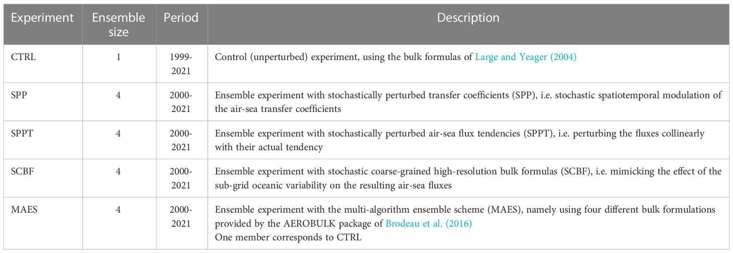
Table 1 List of experiments and main characteristics.
In addition to the 1/4° configuration (CREG025), a very high-resolution (mesoscale-resolving) version of the NEMO model implementation was run for a short 2-year period (2020-2021). Such a configuration, called CREG36, is obtained from the ORCA36 configuration (Bricaud and Castrillo, 2020) similar to CREG025, namely, by flipping the north fold boundary in the Arctic Ocean. This configuration has a 1/36° of spatial resolution and 75 vertical levels and covers the same domain as CREG025. The CREG36 simulation is used to characterize the subgrid variability of CREG025, for use in one of the perturbation schemes presented later (see Section 2.2.3). To this end, we calculate the spatial standard deviation across the CREG36 gridpoints associated with each CREG025 gridpoint (see section 2.2.3). There are no differences between the two configurations except for the horizontal resolution and the timestep duration, and the horizontal diffusivity and viscosity parameters, which are scaled according to the increase in resolution.
2.1.2 Surface boundary conditions and air-sea fluxes
The formulation of the surface boundary conditions in NEMO is as follows: wind stress is used as a surface boundary condition in the computation of the momentum vertical mixing trend. The surface heat flux is divided into two components, the non-solar and the solar heat flux. The non-solar is the non-penetrative part of the heat flux and is used as the surface boundary condition of the first-level temperature model tendency. The solar heat flux is the penetrative component applied as a three-dimensional trend after the light extinction coefficients are calculated as a function of the chlorophyll concentration (Morel and Maritorena, 2001). Finally, the surface freshwater flux is applied as boundary conditions of the first-level salinity model tendency, and as a volume flux in the sea surface height equation. More details of the surface boundary conditions in NEMO can be found in Madec et al. (2017) and Brodeau et al. (2016).
We consider hereafter the air-sea fluxes over the open ocean (namely ice-free or partly ice-covered): no stochastic modulation is added to the air-ice fluxes for sake of simplicity, although this could be added in the future, and because we prefer to assess the net effect of the open ocean air-sea fluxes without any effect from the sea-ice melting cycle. Through the use of bulk formulas, the wind stress vector τ, evaporation E, non-solar (QNS) and solar (QS) heat fluxes and freshwater flux F are given, respectively, by:
with pa being the air density; u10 the 10m wind vector (from which surface currents are subtracted), q and qs the specific humidity and its value at saturation (i.e. at the sea surface), Lv the latent heat of vaporization, cp the ocean heat capacity; θ the potential air temperature, SST the sea surface temperature, δ the emissivity; σ the Stefan-Boltzmann constant, Qsw↓ and Qlw↓ the shortwave and longwave downward fluxes at the surface, α is the open ocean albedo, P the precipitation, and R the incoming freshwater flux from land and ice.
The specific formulation of the transfer coefficients CD, CE and CH (drag, evaporation, and sensible heat coefficients) depends upon the chosen bulk formula. NEMO supports several formulations, implemented following the AEROBULK package (Brodeau et al., 2016; see also section 2.2.5 for details). A previous comparison of these formulations (Bonino et al., 2022) highlights the importance of the drag coefficient computation (for instance its possible dependence on wind speed, and the inclusion of convective gustiness), and the use of skin temperature instead of bulk temperature in the transfer coefficient computation.
It is implicit in the previous formulations that the uncertainty of the surface boundary conditions is due to several concurring factors, i.e. the uncertainty of the atmospheric forcing fields; the uncertainty of the bulk formulation (neutral wind estimation, atmospheric stability estimate, transfer coefficient procedure, etc.), the neglect of several processes (e.g. the contribution of waves in the relative wind), and the effect of the sub-grid variability on the resulting fluxes. In the next section, we introduce several perturbation schemes that aim to simulate one or more of these uncertainty sources.
2.2 Perturbation methods
In this section, we introduce different atmospheric forcing perturbation schemes, which will be evaluated and compared in section 3. We formulate three stochastic schemes, and, for comparison, we also introduce a non-stochastic multi-physics scheme, based on the use of different bulk formulas to form a small ensemble.
2.2.1 Stochastically perturbed transfer coefficients
The first scheme is called stochastically perturbed transfer coefficients, and it is a specific application of the more general stochastically perturbed parameter scheme (SPP, see e.g. Ollinaho et al., 2017; Storto and Andriopoulos, 2021) to the atmospheric boundary perturbation scheme.
The SPP scheme relies on the stochastic spatiotemporal modulation of parameters used within selected numerical schemes; it aims at addressing the uncertainty of the transfer coefficients estimation. The generic parameter p is perturbed using a log-normal distribution:
with the stochastic variable ϵ that follows the normal distribution so that the mean of the perturbed parameter is equal to the unperturbed parameter (Ollinaho et al., 2017). The stochastic modulation relies on the random field ϵ, which is a red-noise field, correlated in space through a first-order Shapiro filter and in time as an AR(1) process, as in Storto and Andriopoulos (2021).
In the SPP scheme, we perturb the three transfer coefficients, so that their perturbed counterparts, actually used in the associated experiments, are given by:
The stochastic field ϵ is the same for the three perturbations, also to ensure that the proportionality between these (e.g. Large and Yeager, 2004) is maintained. After sensitivity tests (see Storto and Andriopoulos, 2021), the decorrelation temporal and spatial scales were set to 10 days and 1000 km.
2.2.2 Stochastically perturbed air-sea flux tendencies
The second scheme revisits the stochastically perturbed parameterization tendencies (SPPT), originally formulated for atmospheric ensemble prediction systems (e.g. Storto et al., 2013), which perturbs the air-sea fluxes collinearly to their tendency. We will refer to such a scheme as stochastically perturbed air-sea flux tendencies, or simply SPPT.
In practice, each flux is perturbed by stochastically modulating its latest time increment, so that:
with the perturbed flux at time t depending on the difference between its unperturbed value and that at the previous model timestep (namely the time increment). Like in most SPPT implementations, perturbations are collinear with the temporal variations, meaning that the largest uncertainty corresponds to cases of very large temporal variations. The stochastic field ϵ is generated as in the SPP scheme: the perturbation follows a Gaussian distribution (unlike the log-normal distribution for perturbations in SPP), with the same temporal and spatial decorrelation scales as in SPP.
2.2.3 Stochastic coarse-grained high-resolution bulk formulas
The third scheme is the stochastic coarse-grained high-resolution bulk formulas (SCBF), which aims at representing explicitly the effect of the ocean subgrid variability on the resulting fluxes. In general, a certain flux f=M(xoc,xatm) can be thought of as a non-linear function of the prognostic ocean state xoc and the prescribed atmospheric state xatm.
The high-resolution computation of bulk formulas implies that a projection operator c- projects the model resolution variables onto a high-resolution grid, and that its pseudo-inverse coarsening operator C (CC−x=x) performs the opposite coarsening operation. Fluxes can then be computed as:
To introduce sub-grid fluctuations, the ocean state on the high-resolution grid CREG36 is perturbed by adding a random fluctuation ϵ with zero mean and standard deviation equal to the subgrid variability so that the perturbed flux is then equal to
This scheme is visually represented in Figure 1. Each gridpoint of the nominal model grid (coarse grid) is decomposed into many sub-gridpoints of the high-resolution grid. Zero-mean random fluctuations of sea surface temperature and currents are added to every sub-gridpoint; then, the bulk formulas are calculated for each sub-gridpoint, and the coarsening operator C is used to map back the high-resolution grid onto the nominal (coarse) model grid.
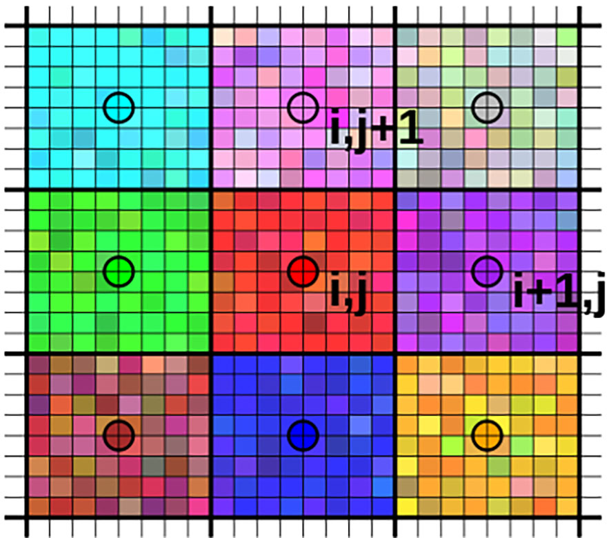
Figure 1 Representation of the SCBF scheme. Each gridpoint in the coarse domain (e.g. CREG025) is represented by the circle. Its gridcell is divided into several sub-gridcells (corresponding e.g. to CREG36). For each of these sub-gridcells, sea surface temperature and current are stochastically modulated according to the spatially varying sub-grid variability. Then, bulk formulas are applied to each sub-gridcell and finally averaged to provide the perturbed value on the coarse grid. Colors symbolically represent different values of e.g. SST.
In our implementation, the arithmetic mean operator is used as a coarsening operator, while the projection operator c- replicates the gridpoint field value over all the sub-gridpoints included in the gridcell. The random fluctuations ϵ are weakly correlated in space and time to mimic coherent subgrid structures (e.g. fronts, filaments, etc.), following an AR(1) process, with a 1 hour and 25 km decorrelation time and space scales, respectively.
The resulting flux perturbations are strictly related to the degree of non-linearity of the bulk formulas, i.e. for perfectly linear formulas the perturbations will be zero by construction; however, the non-linearity and the iterative adjustments that the fluxes and the transfer coefficients depend on (e.g. Large and Yeager, 2004) ensure that perturbations are non-zero and that such perturbations represent in facts the effect of the oceanic sub-grid variability mapped onto the air-sea fluxes.
Sea surface temperature (SST) and current (SSC) subgrid variability is estimated as spatial standard deviation from a 2-year realization of the very high spatial resolution implementation of NEMO at 1/36° of horizontal resolution (CREG36). That is, each gridpoint in the CREG025 configuration is associated with 9x9 sub-gridpoints in CREG36, which are used to calculate the subgrid variability as spatial standard deviations. The spatial standard deviations of SST and SSC are shown in Figure 2. Large values correspond to western boundary currents and the location of the main surface currents in the North Atlantic region.
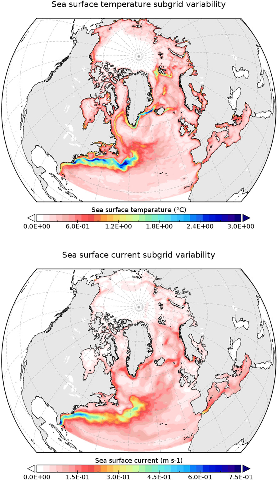
Figure 2 Sea surface temperature (top panel) and current speed (bottom panel) subgrid variability, estimated as spatial standard deviation from a 2-year NEMO simulation at 1/36° of horizontal resolution (CREG36).
2.2.4 Multi-algorithm ensemble scheme
The fourth and last perturbation scheme is inspired by a multi-physics approach, which is a common methodology used in several atmospheric ensemble systems (e.g. Jankov et al., 2005). In practice, four bulk formulation algorithms are used to generate the ensemble, and these are in particular those included in the AEROBULK package (Brodeau et al., 2016): i) the NCEP/CORE bulk formulas (Large and Yeager, 2004); ii) the ECMWF bulk formulas (ECMWF, 2014); iii) the COARE 3.0 algorithm (Fairall et al., 2003); and iv) the COARE 3.5 algorithm (Edson et al., 2013). This perturbation scheme is then called the multi-algorithm ensemble scheme (MAES) and is used in this work mostly for comparison with the stochastic schemes.
Differences between these bulk formulas have been discussed in detail by e.g. Bonino et al. (2022) and reported in section 2.1.3: these are essentially different ways to estimate the air-sea transfer coefficients. In particular, the COARE and the ECMWF formulations are meant to be used with the skin SST through the scheme of e.g. Zeng and Beljaars (2005), while the NCEP/CORE with the bulk SST (namely, in practice, the first model level temperature). Compared to version 3, COARE 3.5 contains, among several upgrades, a refinement of the wind speed dependence of the Charnock coefficient (Edson et al., 2013). Note that here we are not interested in evaluating which transfer coefficient formulation performs better, but to provide different realizations of the formulas.
The MAES scheme has manifold limitations. First, by construction, the ensemble size is limited to the number of available transfer coefficients computation algorithms, which is four in our case. Further algorithms could be implemented; however, this multi-physics scheme is not stochastic, strictly speaking, and the ensemble size is intrinsically limited. Second, the ensemble average is by construction biased compared to the control experiment, which necessarily requires the choice of a certain bulk formula algorithm. In our study, the reference bulk formulas are the NCEP/CORE ones from Large and Yeager (2004), therefore the difference with the MAES ensemble represents only the relative difference in ocean model simulations between such scheme and the mean of all the schemes. Its interpretation is not straightforward and has little importance in the ensemble context, while is however important to identify the impact of a certain bulk formula algorithm.
Nevertheless, the MAES ensemble is used in this study as a reference multi-physics experiment, which is useful to compare with the ensemble spread of the stochastic schemes.
2.2.5 Comparison of perturbations from the schemes
Here, we qualitatively compare the perturbations generated by the schemes to the control experiment for one realization of each scheme at two short time frames (1 day and 1 year, respectively, after model run initialization). Results are given in terms of differences with respect to the control (unperturbed) experiment that shares the same initial conditions for the model integration.
In terms of perturbations on the SST (Figure 3), all schemes show a small impact after one day, in general below 0.05°C. SPP perturbation appears to be the smallest, while SCBF and MAES exhibit a general cooling and warming effect, respectively, in many areas of the domain. After one year of simulation, the perturbations are more developed and lead to differences compared to the control run that exceeds 2°C in correspondence of areas with strong mesoscale activity, such as the Gulf Stream region. All schemes succeed in perturbing the local mesoscale. Elsewhere, SPP and SPPT show negative and positive patterns, while SCBF has a general cooling effect on the SST, and MAES a positive effect. As already mentioned in section 2.2.5, MAES by construction has a non-zero difference of the ensemble mean due to the non-stochasticity of the scheme; in particular, the figure represents the cumulated one-year difference of the COARE 3.0 algorithm compared to the NCEP/CORE bulk formulas.
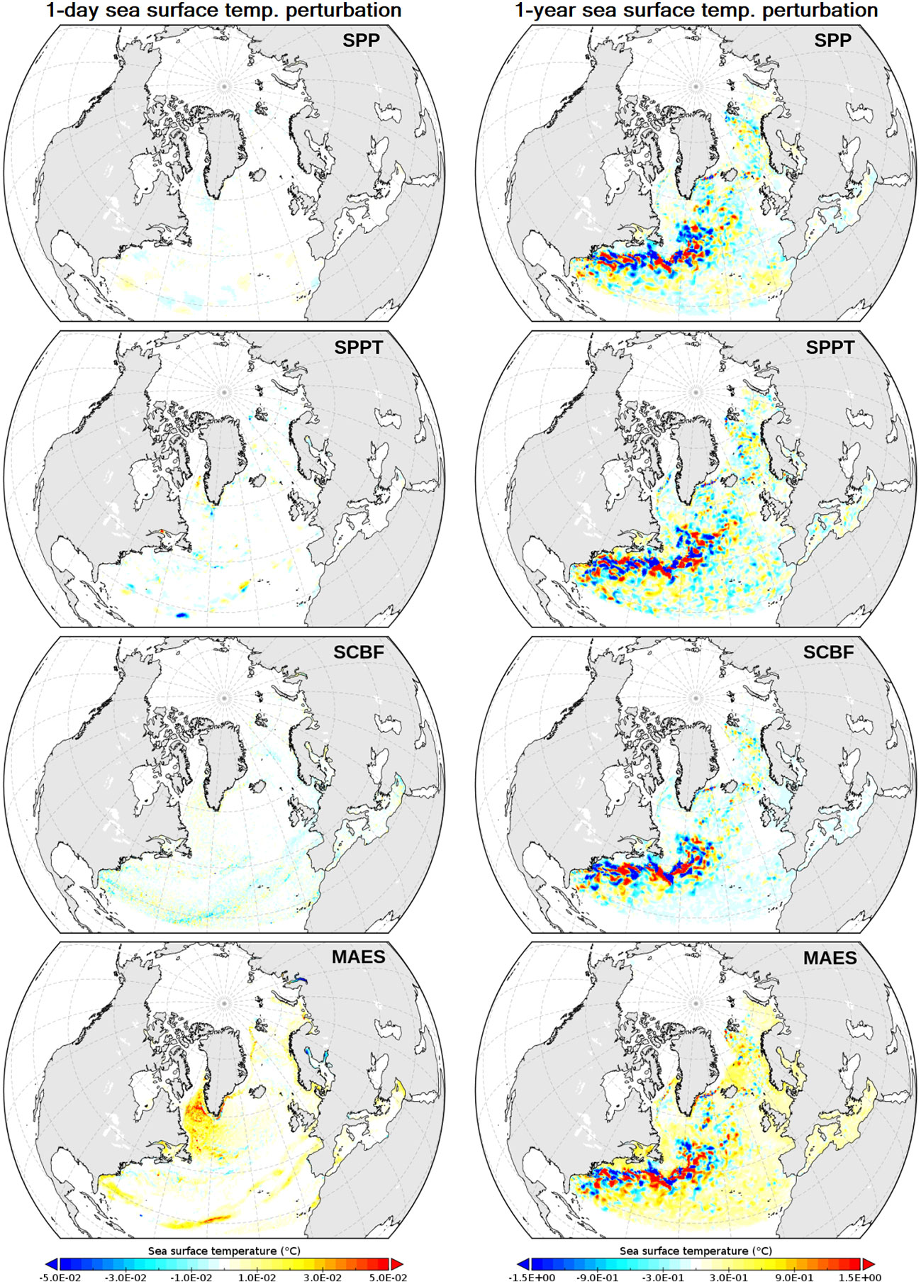
Figure 3 Difference of SST between one perturbed member and the control experiment after one day (left panels) and one year (right panels) from ensemble initialization on 1 January 2000. Each row shows one experiment as described in the text and Table 1. Color bars are different for left and right side panels.
Differences in sea surface height (SSH, Figure 4) indicate very small perturbations at day one (except for the MAES scheme). SCBF shows a very small impact, suggesting that the penetration of the perturbation in the water column is particularly slow with this scheme. After one year of simulation, differences mostly concern the Gulf Stream region.
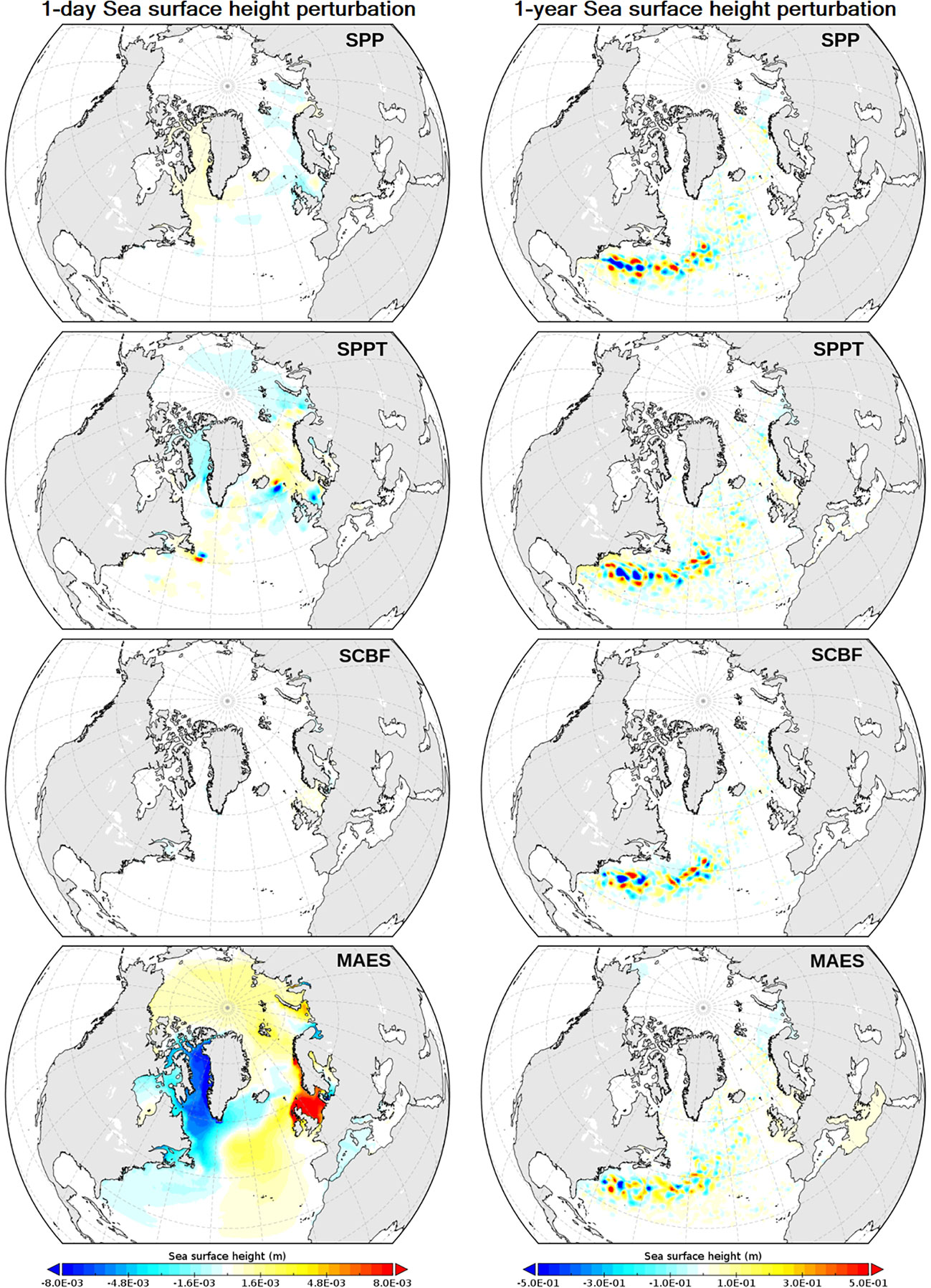
Figure 4 As for Figure 3, but for the sea surface height.
In general, these figures indicate that all schemes require a multi-year time scale to develop into consistent physical patterns, besides the noisy behavior around western boundary current systems. This in turn suggests that the schemes are mostly interesting for multi-year climate-oriented applications, and need to be used in combination with other perturbation schemes (e.g. Storto and Andriopoulos, 2021).
2.3 Experimental design
Four ensemble experiments for the period 2000-2021 have been performed, each ensemble experiment having an ensemble size of 4 members (for a total of 16 simulations and 352 years simulated). We consider the first two years of simulations as an ensemble system spin-up period where the spread ramps up to rather stable values; therefore we focus our analyses on the 20 years 2002-2021 or the 10 years 2012-2021, depending on the specific diagnostic, as specified in the text of section 3. Ensemble experiments are called after their corresponding perturbation scheme, i.e. CTRL (no perturbation, one single realization), SPP, SPPT, SCBF, and MAES. Table 1 summarizes the experiments performed. All the ensemble experiments have been initialized on 1 January 2000 from the CTRL experiment, initialized, in turn, one year before from the GLORYS12 reanalysis.
3 Results
In this section, we show the main results of relevant diagnostics in the North Atlantic and Arctic regions. The ensemble standard deviation (or spread) is only compared between different experiments, namely no study of the ensemble reliability (see e.g. Rodwell et al., 2016) is provided because of the small ensemble size. Additionally, the schemes are conceived to be combined with other perturbation methods that span sub-surface sources of uncertainty. Unless otherwise specified, timeseries are shown for the full 2000-2021 period, while skill scores and climatologies are calculated over 2012-2021, to allow for an ensemble spinup.
3.1 Temperature and salinity
The first assessment of the stochastic air-sea flux experiments concerns the behavior of the temperature and salinity ensemble mean and spread over the study period (2000-2021). This is shown in Figure 5 in terms of area-averaged yearly means of temperature at the sea surface and 100 m of depth, with the seasonal cycle shown aside. For this analysis, we subdivide the CREG025 computational domain into two main areas, the North Atlantic and the Arctic Oceans, whose separation is set at around 60°N. The ensemble means in the North Atlantic region, at both the sea surface and 100 m of depth, show very similar behavior for the five experiments; nevertheless, MAES exhibits a significant, year-round, warm anomaly, while the stochastic coarse-graining algorithm (SCBF) shows a cold anomaly, mainly in winter. Provided that MAES ensemble mean is biased by construction compared to the CTRL experiment, the stochastic coarse-graining algorithm (SCBF) seems the only one to lead to differences in the mean state. This is due to the non-linear relationship between sea-surface temperature and fluxes; for instance, a zero-mean perturbation to the SST can lead to an increase of outgoing longwave radiation, namely, to heat loss and negative anomalies, due to non-linearity of the blackbody radiation equation. Other effects can eventually dominate locally. SCBF cold anomalies dominate most of the Gulf Stream Region (not shown).
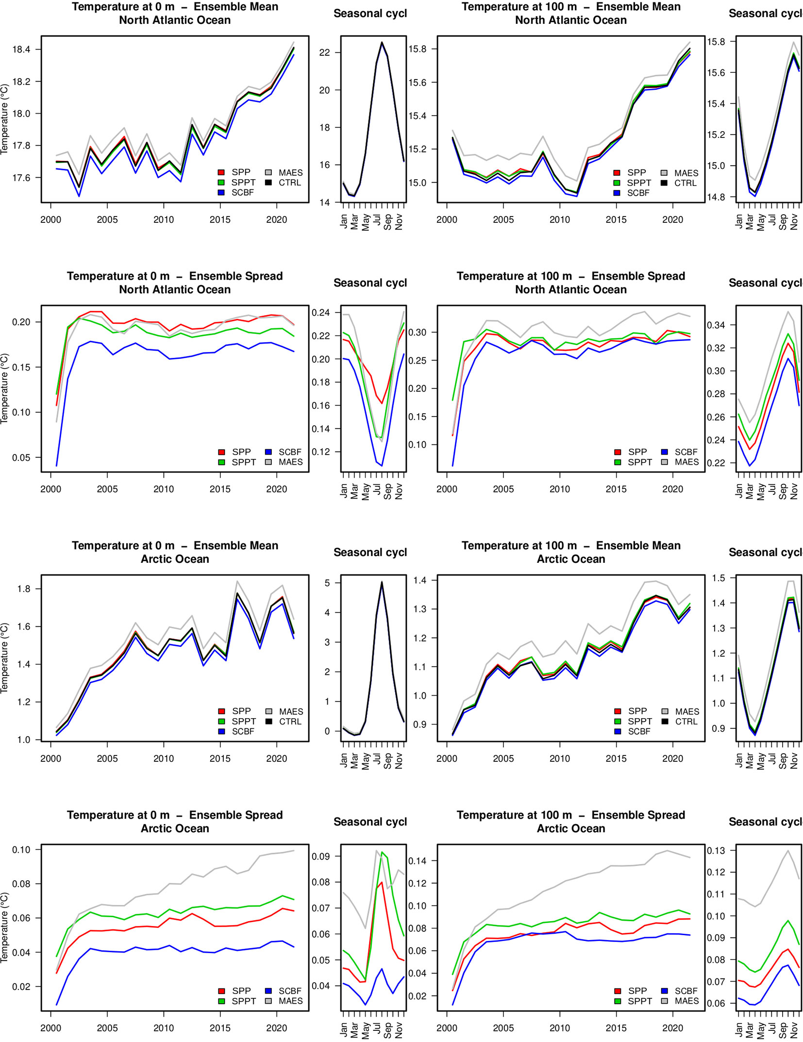
Figure 5 Timeseries (yearly means and monthly climatology) of temperature ensemble mean and spread at the sea surface and 100 m of depth, for the two regions North Atlantic (south of 60°N) and Arctic (north of 60°N) Oceans.
In terms of ensemble spread, at the sea surface, MAES and the stochastically perturbed transfer coefficients (SPP) provided the largest values after a 2-year ensemble spinup. Interestingly, the seasonal cycle does not show a perfect offset; for instance, SPP has a larger spread in summer than the other experiments, while providing a median value in summer. At 100 m of depth, MAES exhibits the largest spread, stressing the dispersion in the sub-surface given by the multi-algorithm scheme. In general, the ensemble spread increases with stratification conditions.
Qualitatively similar results hold for the Arctic region. However, the spread panels show MAES having the largest values at both 0 and 100 m of depth. The seasonality of the sea surface temperature spread has complex behavior, peaking in general in summer due to a larger portion of the Arctic Ocean being ice-free compared to winter. At 100 m of depth, the effect of the stratification prevails again, and the spread peaks around September.
Area-averaged profiles (Supplementary Figure 1) of temperature confirm the relatively small differences compared to the CTRL experiment in terms of the ensemble mean. In the North Atlantic Ocean, the ensemble spread is larger than the Arctic one, with the experiments exhibiting similar values. Especially in the Arctic Ocean, the spread increases gradually in correspondence with the intrusion of the North Atlantic waters; there are larger values in the sub-surface than at the surface because perturbations penetrate deeper while the sea surface is balanced with the atmospheric state. However, in both basins, the ensemble spread drops below the 40th model level (500 m of depth), due to the relatively short period for the perturbation to penetrate the deep and abyssal oceans (not shown). In the Arctic Ocean, however, MAES has a larger spread than the other ensemble experiments, at all depths and in both seasons.
Figure 6 shows the same diagnostic as Figure 5, but for salinity. An opposite signal to that of temperature is visible in the North Atlantic Ocean, where MAES exhibits a fresh anomaly and SCBF a salty anomaly. The ensemble spread suggests that for all regions and depths, MAES has the largest values, which drop below 300 m depth (Supplementary Figure 2). Note that in the Arctic Ocean, the spread seems not stable even at 100 m after the 20-year simulation period, indicating that for salinity, likely due to the sea-ice cycle, the spread requires long periods to stabilize based on these stochastic air-sea flux schemes.
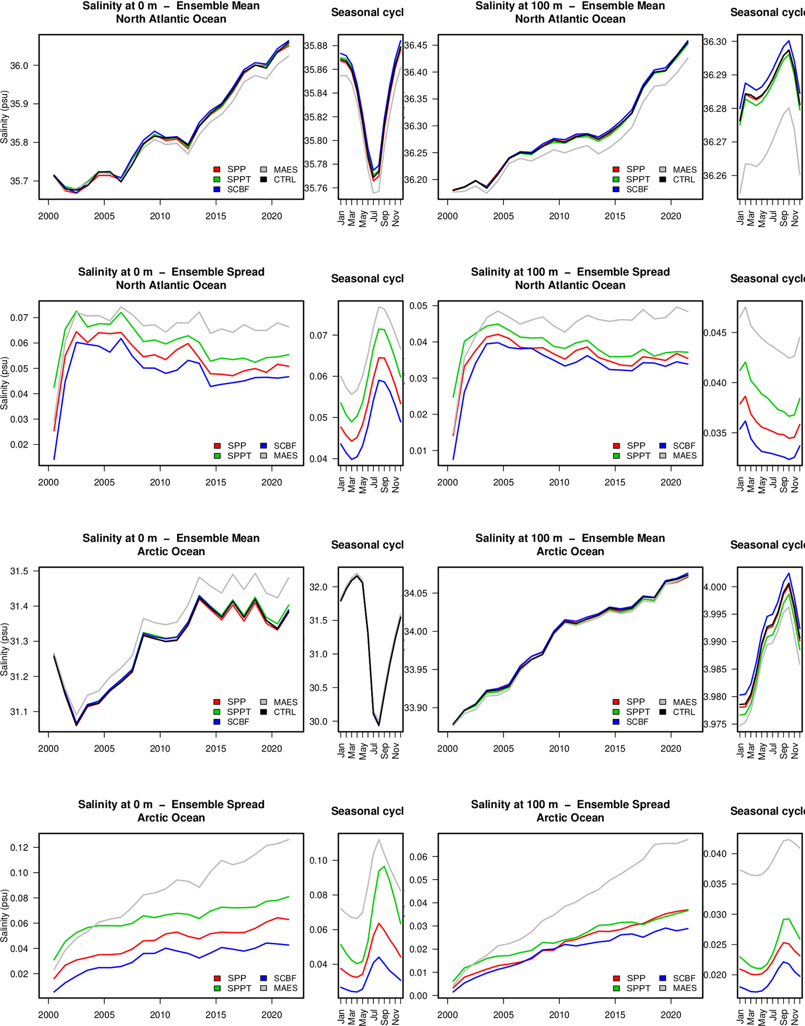
Figure 6 As for Figure 5, but for salinity.
Verification of the experiments can be performed against independent SST analyses, provided by the UKMO OSTIA analysis system (Donlon et al., 2012). Summary results are shown in Figure 7, in terms of zonally averaged anomaly (with respect to the CTRL experiment), RMSE versus OSTIA SST, and RMSE percent decrease compared to the CTRL experiment. MAES and SCBF have warm and cool anomalies up to 75°N (except for MAES in the 50°-55° layer). However, in terms of RMSE, all experiments lead to statistically significant improvements of SST RMSE between 30 and 55°N in the North Atlantic Ocean. The patterns north of 55°N are more complex. MAES maxima of SST RMSE reach up to 10% in selected latitudinal bands, and are equal to 2.7% as domain-averaged, against SCBF (2.4%), SPPT (1.9%), and SPP (1.2%). These results suggest that the stochastic schemes, even with a small ensemble size, provide non-negligible improvements to the sea surface skill scores.
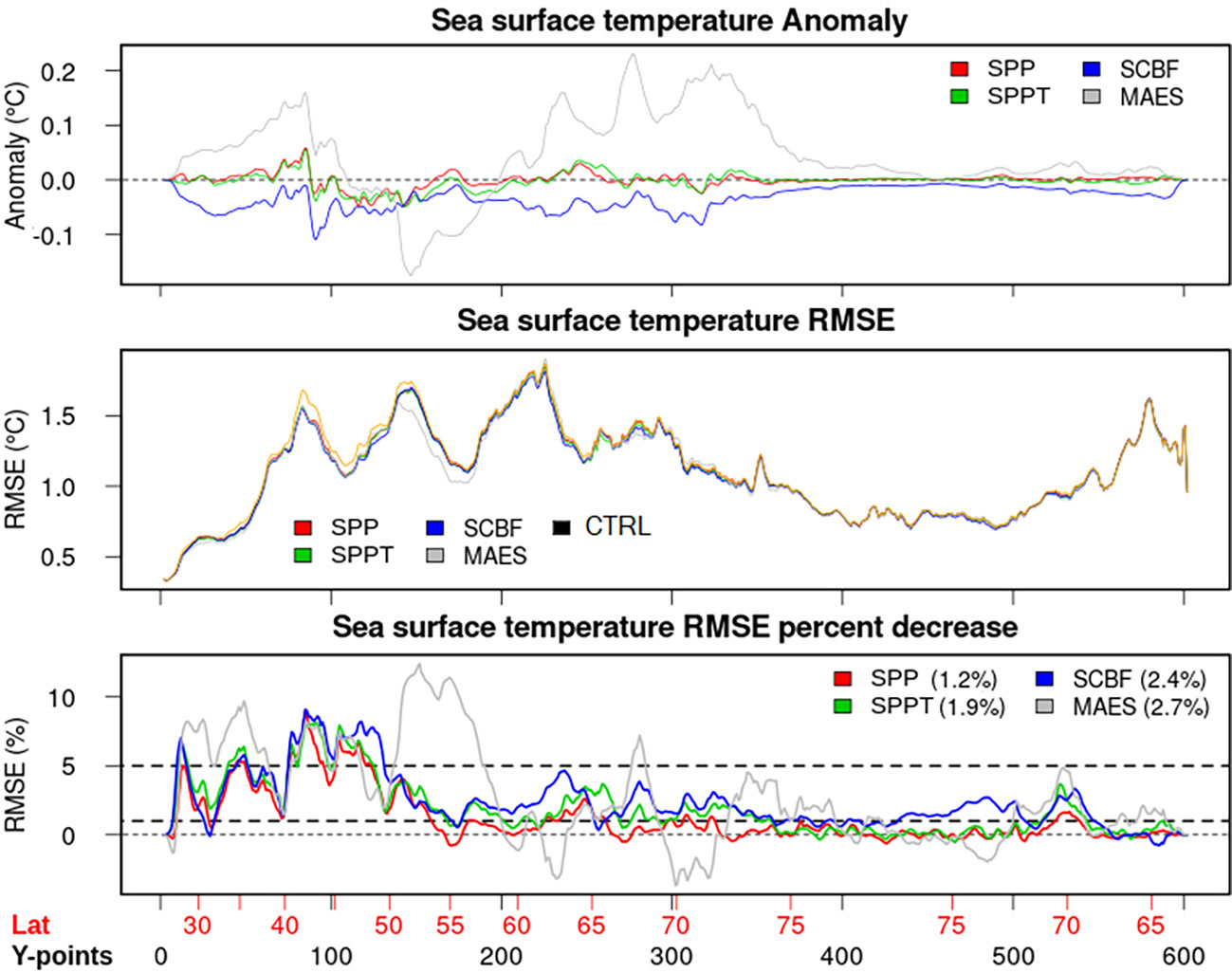
Figure 7 Sea surface temperature anomaly (difference compared to CTRL, top panel) and RMSE (middle panel) against the UKMO OSTIA daily SST analyses (Donlon et al., 2012), and RMSE percent decrease (bottom panel) compared to the CTRL experiment. The legend of the bottom panel reports the domain-averaged RMSE percent decrease. The x-axis reports the y-coordinate of the model as statistics are computed over the native model domain geometry, while red numbers show the corresponding zonally averaged latitudes (which are increasing in the Atlantic Ocean until reaching the North Pole and then decreasing until the Bering Strait).
Then, we focus on the 2012-2021 differences in mixed layer depth (MLD) during March, where MLD is the largest, especially in the deep convection regions of the Labrador Sea and subpolar gyre (e.g. Rühs et al., 2021). This diagnostic is important in the North Atlantic and Arctic regions, especially for their pumping effect on the thermohaline circulation (DanabasogluCoauthors, 2016; Storto et al., 2016). These deep convection areas have MLD that exceeds 3000 m for the 2012-2021 average (Figure 8). All the ensemble experiments except SCBF show enhanced deep convection in the Greenland Sea. SCBF shows instead shallower MLD in this region, which is likely linked to the displacement of the sea-ice edge (and related freshwater input) towards the middle of the Greenland Sea, thus enhancing stratification therein. Patterns in the Labrador Sea and nearby regions are somehow more complicated to interpret, with MAES showing a shallower MLD in the western part of the deep convection region and a deeper MLD in the eastern part. However, these differences are important to explain possible changes in the North Atlantic low-frequency circulation.
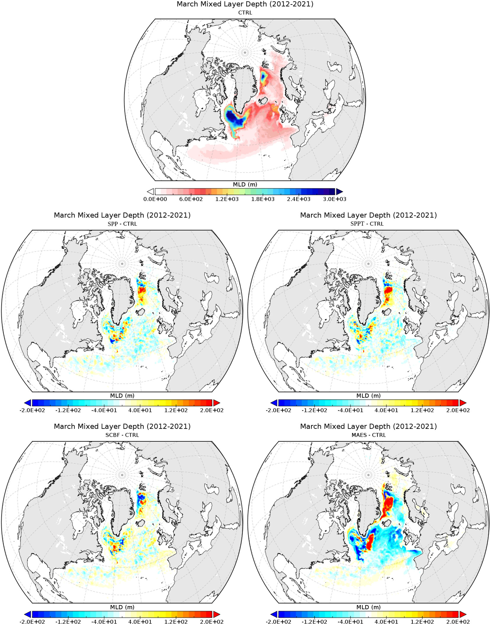
Figure 8 Climatological March mixed layer depth (2012-2021) for the CTRL experiment (top panel) and the difference between the ensemble mean and the CTRL experiments for each stochastic experiment (middle and bottom panels). The mixed layer depth is defined here as the depth where the density difference with the 10 m value exceeds 0.01 Kg m-3 (see e.g. Toyoda et al., 2017, for a discussion on the different definitions).
Figure 9 reports the 2012-2021 averaged March profiles of temperature in the two deep convection areas, showing as reference the EN4 objective analyses (Good et al., 2013) for the same month, period, and region. In the subpolar gyre region, EN4 shows a warmer profile in the top 200 m, with a much sharper thermocline below than the ensemble experiments. Only MAES approaches EN4 in the top 50 m, suggesting that some bulk formula other than the NCEP/CORE (Large and Yeager, 2004) performs significantly better in the region. SPP and SPPT also provide a slight improvement compared to CTRL. An opposite situation occurs in the Labrador Sea, with the experiments being warmer than the objective analyses; also here, MAES performs better.
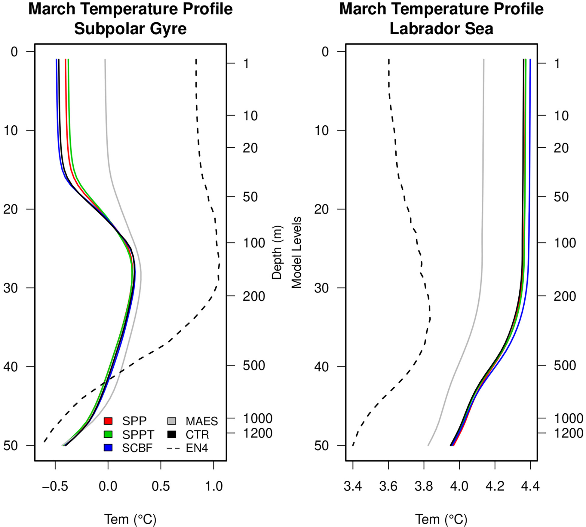
Figure 9 Mean March temperature profiles for the CTRL experiment and the ensemble means of the experiments, over the subpolar gyre (defined as the area 15°W-6°W; 68°N-77°N) and the Labrador Sea (defined as the area 57°W-37°W; 50°N-60°N) deep convection regions. For reference, also shown are the profiles from the UKMO EN4 objective analyses (Good et al., 2013).
3.2 Circulation, eddy kinetic energy, and mesoscale activity
Next, we analyze the difference in surface and integrated circulation implied by the air-sea flux stochastic schemes. First, we have validated the surface current speed against independent drifter-derived 6-hourly current speed, provided by the Global Drifter Program of NOAA (Lumpkin et al., 2013), during the period 2016-2021 (the latest 6 years of experiments). The use of the stochastic schemes has, in general, a non-negligible impact on the surface current speed, except for the Mediterranean Sea region, where the impact is very small. Both the North Atlantic and Arctic portions of the domain exhibit improvements of the order of 1.8-3% in RMSE compared to the control experiments. In particular, SPP, SPPT, and SCBF show all statistically significant improvements in the North Atlantic and Arctic regions, with SPPT (stochastically perturbed air-sea flux tendencies) exhibiting the largest improvement, equal to 3% in both regions and 1.8% over the entire domain. The results are summarized in Table 2.
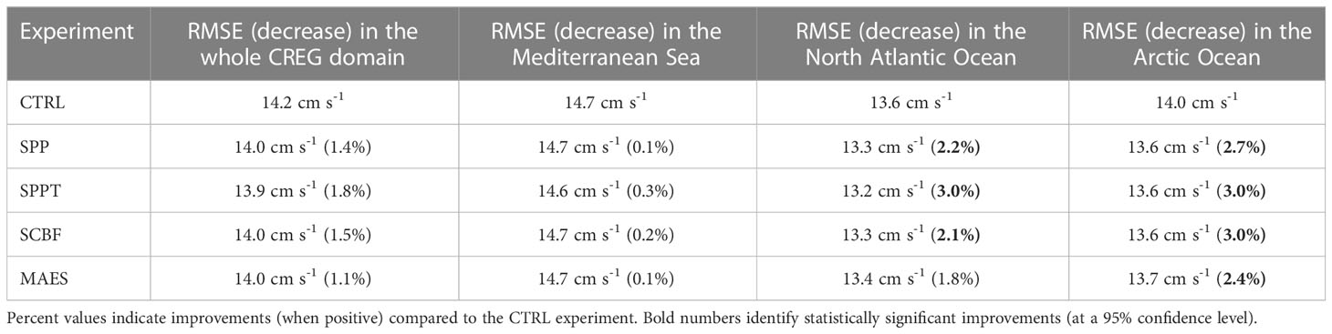
Table 2 Verification metrics (RMSE) of surface current speed (the speed at 15m depth) against drifters from the Global Drifter Program of NOAA AOML (Lumpkin et al., 2013).
The integrated circulation, in terms of the barotropic streamfunction (BSF) for the CTRL experiment, shows (top panel of Figure 10) the typical structure (see e.g. Colin de Verdière and Ollitrault, 2016) with positive values in the North Atlantic subtropical gyre and maxima corresponding to the Gulf Stream main path, and negative values in the subpolar gyre with minima near Labrador Sea entrance (the signs being arbitrary, and depending on the integration initialization). Differences in the ensemble mean from the stochastic experiments (middle and bottom panels of Figure 10), compared to the CTRL experiment, highlight the complex structure around the Gulf Stream separation and path; indeed, the dipolar structures indicate the shift of the main current path. However, all experiments show a consistent increase in barotropic streamfunction near the Labrador Sea entrance and a decrease towards the Denmark Strait.
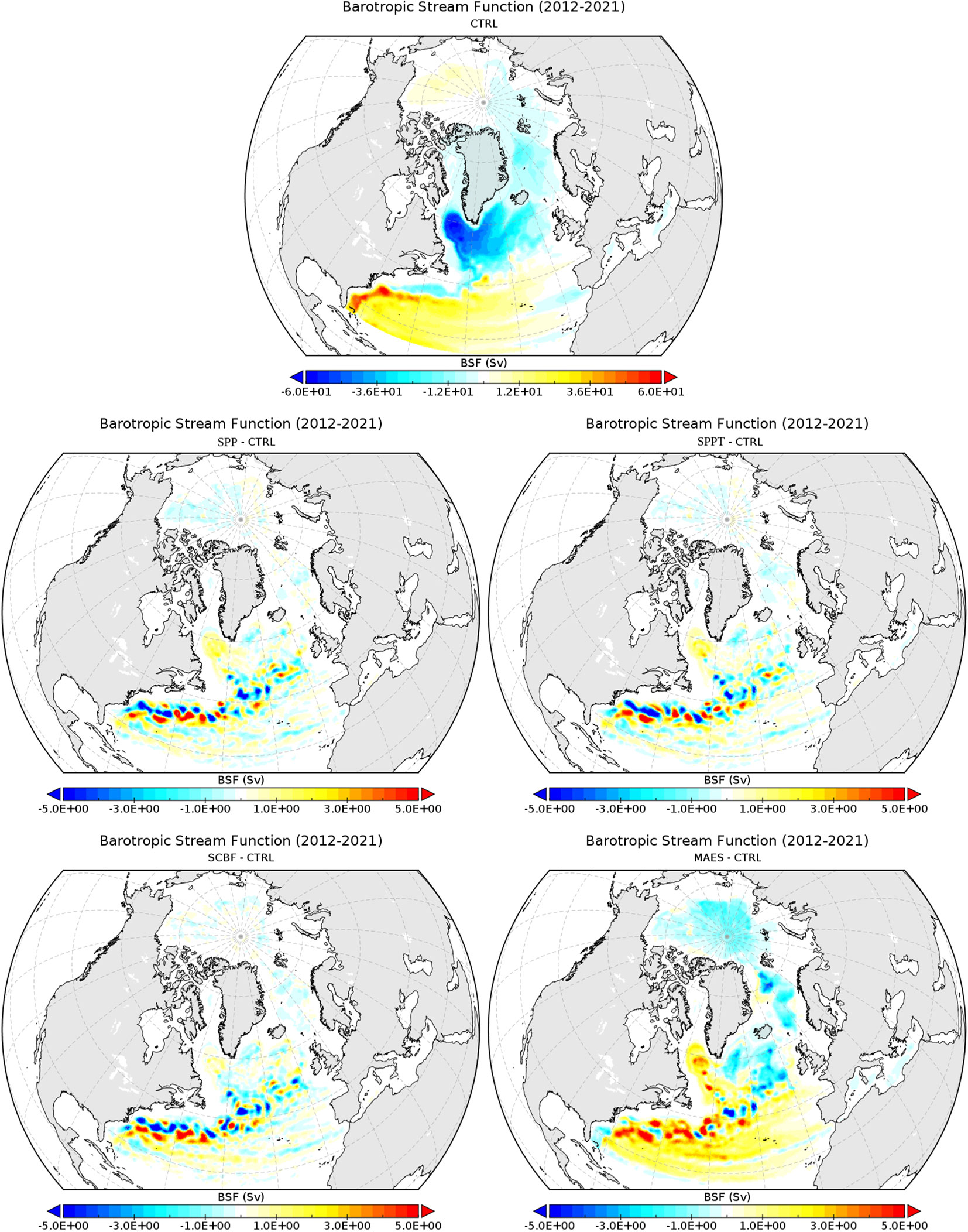
Figure 10 As for Figure 8, but for the barotropic stream function, calculated through the CDFTOOLS (available at https://github.com/meom-group/CDFTOOLS).
To quantify the effects of the scheme on the large-scale gyre circulation, Figure 11 reports the value of the gyre indexes for the subpolar (SPG) and subtropical (STG) gyres, together with their percent variation compared to the CTRL experiment. The gyre indexes are defined as follows: for the SPG it is the minimum BSF between 65° and 40°W at 53°N; while the STG index is derived as the maximum BSF between 80° and 60°W at 34° (e.g. DanabasogluCoauthors, 2014). There occurs a consistent decrease of both gyre strengths, with the subpolar strength decrease ranging from 0% (SCBF) to -6% (MAES) and the subtropical gyre decrease from -5% (MAES) to -8% (SCBF), with other experiments lying in between. The two gyre decreases tend to compensate each other to some extent in the experiments, i.e. the experiments show favorite gyre strength decrease but not simultaneous across SPG and STG. Note also that observation-based estimates for the SPG gyre strength suggest values between 37 and 42 Sv (Xu et al., 2013), which are smaller than the CTRL experiment. This indicates that the air-sea stochastic physics schemes mitigate, to a small extent, the overestimation of the gyre circulation in the unperturbed experiment.
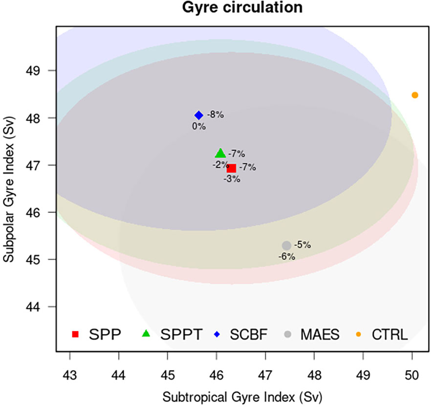
Figure 11 Subtropical and subpolar gyre indexes ensemble mean (points) and spread (shaded ellipses) for the CTRL and the ensemble experiments. The indexes are defined as the minimum BSF between 65° and 40°W at 53°N (SPG), and the maximum BSF between 80° and 60°W at 34° (STG) (Danabasoglu and Coauthors, 2014). Percent values to the right (bottom) indicate the percent variation of the STG (SPG) compared to the CTRL experiment.
Stochastic physics schemes may lead to an increase in eddy kinetic energy (EKE) and mesoscale activity, due to the rectification of the energy cascade implied by the enhanced subgrid variability (e.g. Perezhogin, 2019). This is evident in eddy-permitting resolution models but occurs also in higher-resolution configurations (StortoAndriopoulos, 2021). To this end, we have investigated the change in EKE, compared to the CTRL experiment, implied by the air-sea flux stochastic schemes. In the experiments, looking at the zonally averaged values of eddy kinetic energy during the 2012-2021 period (Figure 12), the EKE peaks at around 35°N (eddy-rich areas), roughly near the north of the Gulf Stream separation, and decreases polewards. Ensemble experiments generally lead to an increase of EKE, with similar characteristics in the band 26-55°N among the experiments (except MAES which shows an average decrease of EKE in this latitudinal band). North of 55°N, both SPPT, and MAES exhibit an increase of EKE of the order 5-15%, and, globally, the perturbation of the air-sea flux tendencies (SPPT) leads to the largest EKE increase, equal to 4.4%. EKE spread (bottom panel of Figure 12) indicates some non-negligible dispersion of the EKE values, generally below the increase itself, which follows the poleward decrease of EKE. This indicates that a likely larger ensemble than 4 members is needed to assess the effect of the EKE increase in the ensemble mean compared to the ensemble dispersion. Nevertheless, the effect is non-negligible and particularly evident in the Arctic region for the SPPT experiment, which owns smaller dispersion than MAES.
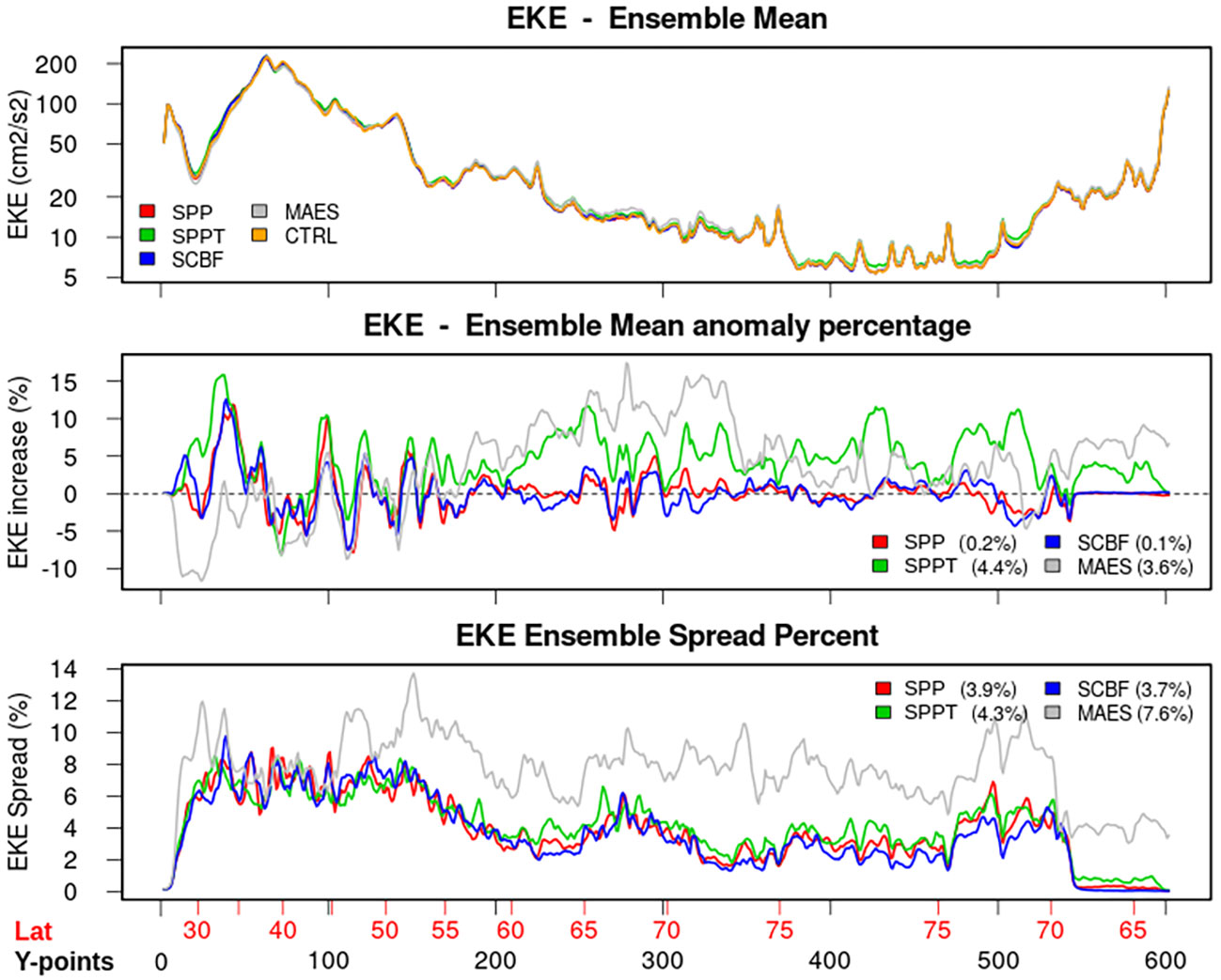
Figure 12 Zonally averaged eddy kinetic energy (EKE) from the CTRL experiment and the ensemble means (top panel), its difference compared to the CTRL experiment (middle panel), and the EKE spread, shown as percent of the ensemble mean value (bottom panel). The legends of the middle and bottom panels report the domain-averaged values. EKE is calculated from the geostrophic velocities, estimated in turn from the sea surface height. The x-axis is defined in Figure 7.
3.3 North Atlantic transports
Combined effects on the mesoscale activity, seawater properties, and large-scale circulation may imply a different redistribution of heat in the North Atlantic Ocean, which is a crucial diagnostic for several climate-impacting processes (e.g. Arctic sea-ice decline, Docquier and Koenigk, 2021). To this end, we compare the meridional heat transports among the different stochastic experiments and with respect to the CTRL experiment. This is shown in Figure 13 in terms of zonally and temporally (2012-2021) averaged meridional heat transport (MHT) values. The top panel shows the ensemble mean values as a function of latitude or y-axis; observational estimates are reported for comparison with circles (from Ganachaud and Wunsch, 2000, and Lumpkin and Speer, 2007; see the caption of Figure 13 for details). The middle panel shows the percent anomalies of the ensemble experiments compared to CTRL (percent difference of the ensemble mean with respect to CTRL). Compared to the observational estimates, CTRL values appear overestimated south of 60°N and underestimated at 68°N. However, the observational estimates were calculated from a dataset much older than the simulated periods, and the temporal variability may also contribute to the discrepancies. The observational estimates are reported only for reference rather than quantitative validation. For instance, compared to the OSNAP east section (~60°N in the North Atlantic, see e.g. Li et al., 2021) over the same period 2014-2018, the MHT values are close enough to the observed value of 0.43 PW for the 2014-2018 period, with all ensemble experiments and the CTRL being equal to 0.44 PW, except MAES (0.45 PW). This means that MHT values are in agreement with observed estimates when compared for the same period, and their relative difference is small.
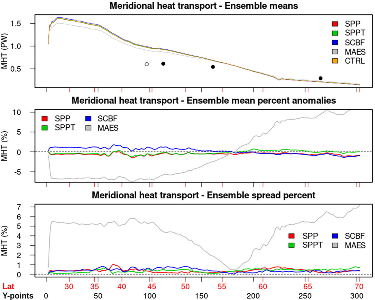
Figure 13 Meridional heat transport for the CTRL end the ensemble means of the stochastic experiments (top panel), its percent anomaly compared to the CTRL experiment (middle panel), and the ensemble spread (bottom panel), shown as percent value compared to the ensemble mean. The x-axis is defined in Figure 7. The top panel also reports the estimates from Ganachaud and Wunsch (2000) (empty circle) and Lumpkin and Speer (2007) (solid circles).
The multi-algorithm ensemble scheme (MAES) shows a slowdown in the poleward transport south of ~55°N (up to -5%), consistent with the cold anomaly and the weakened subtropical gyre strength. SCBF, on the contrary, shows a slight increase of MHT, of the order of 1-2% south of 50°N. The other experiments show a rather neutral difference. In the Arctic, between 60°N and 70°N, MAES exhibits an increase of MHT, consistent, again, with the warm anomalies in the Labrador Sea and north of it. The ensemble spread is generally very small for all experiments (below 1% of the ensemble mean value), except for MAES where it approaches 6% south of 45°N. This means that the stochastic physics schemes only marginally affect the heat redistribution in the North Atlantic Ocean, except when the multi-algorithm ensemble is adopted, because of the improvements in the hydrographic characterization of individual bulk formulas, especially in the areas of deep convection.
4 Discussion
In this work, we investigate different approaches to enable a probabilistic representation of the ocean model, focusing on the perturbation of the air-sea fluxes. In general, the perturbation of the air-sea fluxes should be conceived in combination with other perturbation or ensemble generation methods that span the uncertainty associated with subsurface physics (e.g. Storto and Andriopoulos, 2021). Nevertheless, while customary methods for perturbing the atmospheric forcing rely on atmospheric input data perturbations (e.g. Zuo et al., 2019), here we formulate new stochastic schemes aiming at accounting for the uncertainty in the air-sea flux formulation. This appears important for long-term simulations and reanalyses, and coupled prediction systems. In particular, extended-range prediction systems generally benefit from stochastic physics developments achieved independently in e.g. the oceanic and atmospheric communities (see e.g. Berner et al., 2017), which neglect, in most cases, the uncertainty in the air-sea interface physics. Indeed, the schemes we present here may be fruitfully implemented in long-range coupled prediction systems.
We formulate the problem of stochastically addressing the air-sea flux uncertainty by introducing three different stochastic schemes: i) the stochastic modulation of air-sea transfer coefficients (SPP), inspired by the commonly adopted stochastic perturbation of parameter (Ollinaho et al., 2017); ii) the stochastic perturbation of the flux tendencies (SPPT), inspired by the stochastic perturbation of parametrization tendencies (Buizza et al., 1999); and iii) a stochastic coarse-grained high-resolution bulk formulas (SCBF), which aims at representing the effect of the ocean subgrid variability on the resulting air-sea fluxes. Additionally, we consider a multi-algorithm ensemble scheme (MAES), where different members are associated with different bulk formulas. The schemes are implemented in a regional configuration of the NEMO model over the North Atlantic and Arctic Oceans and the Mediterranean Sea. The performances of the schemes are compared in a series of 22-year 4-member ensemble experiments, each one with a different perturbation scheme,
The schemes lead to different ocean responses in terms of seawater properties, large-scale ocean circulation, mesoscale activity, and meridional heat redistribution, The choice of the scheme for implementation in forecasting or reanalysis systems depends on the specific application, and we summarize the main outcomes of our work below.
The SPP scheme is rather simple to implement and provides only slight improvements in the verification skill scores (drifter current speed, SST analyses, vertical profiles of temperature from objective analyses) but a quite large ensemble spread in the North Atlantic region, comparable at the surface with the MAES. SPPT has good verification skill scores compared to the CTRL experiment, is in general unbiased with moderate ensemble spread, and leads to the largest increase in eddy kinetic energy, making it appealing for several applications oriented to enhancing the mesoscale activity. SCBF is the most novel scheme, which provides the largest improvements in the SST, and ocean current speed; however, it provides a small ensemble spread and EKE increase, and leads to non-negligible biases compared to the CTRL experiment, with cold and salty anomalies. The MAES scheme can be used only in small ensemble sizes, naturally limited by the finite number of possible bulk formula algorithms; moreover, it is biased by construction compared to a reference simulation that necessarily requires the choice of a bulk formula. Nevertheless, it leads to the largest ensemble spread and provides different realistic realizations of the model integration. The rectification of the ensemble mean compared to the CTRL in many aspects is however coincidental, in the sense that is a consequence of the choice of the reference simulation configuration. Combining MAES with multiple physics in ocean models will help design a reliable ensemble system.
The development of these schemes will also help introduce stochastic elements in ocean forecasting systems, to extend the predictability horizon of eddies and other relevant processes. Future investigations will include assessing the schemes in the context of a coupled Earth System model.
Data availability statement
The raw data supporting the conclusions of this article will be made available by the authors, without undue reservation.
Author contributions
All authors listed have made a substantial, direct, and intellectual contribution to the work and approved it for publication.
Acknowledgments
Acknowledgment is made for the use of ECMWF’s computing and archive facilities in this research. The initial developments of the STOPACK stochastic physics package were supported by the ERGO project (Copernicus Climate Change Service contract C3S_321b).
Conflict of interest
The authors declare that the research was conducted in the absence of any commercial or financial relationships that could be construed as a potential conflict of interest.
Publisher’s note
All claims expressed in this article are solely those of the authors and do not necessarily represent those of their affiliated organizations, or those of the publisher, the editors and the reviewers. Any product that may be evaluated in this article, or claim that may be made by its manufacturer, is not guaranteed or endorsed by the publisher.
Supplementary material
The Supplementary Material for this article can be found online at: https://www.frontiersin.org/articles/10.3389/fmars.2023.1155803/full#supplementary-material
References
Andrejczuk M., Cooper F. C., Juricke S., Palmer T. N., Weisheimer A., Zanna L. (2016). Oceanic stochastic parameterizations in a seasonal forecast system. Monthly Weather Rev. 144 (5), 1867–1875. doi: 10.1175/MWR-D-15-0245.1
Barnier B., Madec G., Penduff T., Molines J.-M., Treguier A.-M., Le Sommer J., et al. (2006). Impact of partial steps and momentum advection schemes in a global ocean circulation model at eddy-permitting resolution. Ocean Dynamics 56, 543–567. doi: 10.1007/s10236-006-0082-1
Barth A., Canter M., Van Schaeybroeck B., Vannitsem S., Massonnet F., Zunz V., et al. (2015). Assimilation of sea surface temperature, sea ice concentration and sea ice drift in a model of the southern ocean. Ocean Model. 93, 22–39. doi: 10.1016/j.ocemod.2015.07.011
Berner J., Achatz U., Batté L., Bengtsson L., Cámara A., Christensen H. M., et al. (2017). Stochastic parameterization: Toward a new view of weather and climate models. Bull. Am. Meteorological Soc. 98 (3), 565–588. doi: 10.1175/BAMS-D-15-00268.1
Bonino G., Iovino D., Brodeau L., Masina S. (2022). The bulk parameterizations of turbulent air-sea fluxes in NEMO4: the origin of sea surface temperature differences in a global model study. Geosci. Model. Dev. 15, 6873–6889. doi: 10.5194/gmd-15-6873-2022
Bricaud C., Castrillo M. (2020). Overview of the first year of the NEMO global 1/36° configuration (ORCA36) development. EGU Gen. Assembly 2020, EGU2020–22147. doi: 10.5194/egusphere-egu2020-22147
Brodeau L., Barnier B., Gulev S., Woods C. (2016). Climatologically significant effects of some approximations in the bulk parameterizations of turbulent air-sea fluxes. J. Phys. Oceanogr. 47 (1), 5–28. doi: 10.1175/JPO-D-16-0169.1
Buizza R., Miller M., Palmer T. N. (1999). Stochastic representation of model uncertainties in the ECMWF ensemble prediction system. Q. J. R. Meteorological Soc. 125 (560), 2887–2908. doi: 10.1002/qj.49712556006
Colin de Verdière A., Ollitrault M. (2016). A direct determination of the world ocean barotropic circulation. J. Phys. Oceanogr. 46 (1), 255–273. doi: 10.1175/JPO-D-15-0046.1
Danabasoglu G., Coauthors (2014). North Atlantic simulations in coordinated ocean-ice reference experiments phase II (CORE-II). part I: Mean states. Ocean Modell. 73, 76–107. doi: 10.1016/j.ocemod.2013.10.005
Danabasoglu G., Coauthors (2016). North Atlantic simulations in coordinated ocean-ice reference experiments phase II (CORE-II). part II: Inter-annual to decadal variability. Ocean Modell. 97, 65–90. doi: 10.1016/j.ocemod.2015.11.007
Docquier D., Koenigk T. (2021). A review of interactions between ocean heat transport and Arctic sea ice. Environ. Res. Lett. 16, 123002. doi: 10.1088/1748-9326/ac30be
Donlon C. J., Martin M., Stark J. D., Roberts-Jones J., Fiedler E. (2012). The operational Sea surface temperature and Sea ice analysis (OSTIA) system. Rem. Sens. Environ. 116, 140–158. doi: 10.1016/j.rse.2010.10.017
Dupont F., Higginson S., Bourdallé-Badie R., Lu Y., Roy F., Smith G. C., et al. (2015). A high-resolution ocean and sea-ice modelling system for the Arctic and north Atlantic oceans. Geosci. Model. Dev. 8, 1577–1594. doi: 10.5194/gmd-8-1577-2015
ECMWF (2014) IFS documentation–Cy40r1. operational implementation 22 November 2013. part IV: Physical processes (ECMWF). Available at: http://www.ecmwf.int/sites/default/files/IFS_CY40R1_Part4.pdf (Accessed April 2016).
Edson J. B., Jampana V., Weller R. A., Bigorre S. P., Plueddemann A. J., Fairall C. W., et al. (2013). On the exchange of momentum over the open ocean. J. Phys. Oceanogr. 43 (8), 1589–1610. doi: 10.1175/JPO-D-12-0173.1
Fairall C. W., Bradley E. F., Hare J. E., Grachev A. A., Edson J. B. (2003). Bulk parameterization of air-sea fluxes: Updates and verification for the COARE algorithm. J. Climate 16, 571–591. doi: 10.1175/1520-0442(2003)016<0571:BPOASF>2.0.CO;2
Flather R. A. (1994). A storm surge prediction model for the northern bay of Bengal with application to the cyclone disaster in April 1991. J. Phys. Oceanogr. 24, 172–190. doi: 10.1175/1520-0485(1994)024<0172:ASSPMF>2.0.CO;2
Ganachaud A., Wunsch C. (2000). Improved estimates of global ocean circulation, heat transport and mixing from hydrographic data. Nature 408, 453–457. doi: 10.1038/35044048
Good S. A., Martin M. J., Rayner N. A. (2013). EN4: quality controlled ocean temperature and salinity profiles and monthly objective analyses with uncertainty estimates. J. Geophys. Res.: Oceans 118, 6704–6716. doi: 10.1002/2013JC009067
Hersbach H., Bell B., Berrisford P., Hirahara S, Horányi A, Muñoz-Sabater J, et al. (2020). The ERA5 global reanalysis. Q J. R Meteorol Soc 146, 1999–2049. doi: 10.1002/qj.3803
Jankov I., Gallus W. A. Jr., Segal M., Shaw B., Koch S. E. (2005). The impact of different WRF model physical parameterizations and their interactions on warm season MCS rainfall. Weather Forecasting 20 (6), 1048–1060. doi: 10.1175/WAF888.1
Juricke S., MacLeod D., Weisheimer A., Zanna L., Palmer T. N. (2018). Seasonal to annual ocean forecasting skill and the role of model and observational uncertainty. Q J. R Meteorol Soc 144, 1947–1964. doi: 10.1002/qj.3394
Large W. G., Yeager S. G. (2004). “Diurnal to decadal global forcing for ocean and sea-ice models: the data sets and flux climatologies,” in NCAR Technical report NCAR/TN-460, Boulder, Colorado, USA: National center for Atmospheric Research. doi: 10.5065/D6KK98Q6
Lellouche J.-M., Greiner E., Bourdallé-Badie R., Garric G., Melet A., Drévillon M., et al. (2021). The Copernicus global 1/12° oceanic and Sea ice GLORYS12 reanalysis. Front. Earth Sci. 9. doi: 10.3389/feart.2021.698876
Li F., Lozier M. S., Bacon S., Bower A.S., Cunningham S. A., Jong M. F., et al. (2021). Subpolar north Atlantic western boundary density anomalies and the meridional overturning circulation. Nat. Commun. 12, 3002. doi: 10.1038/s41467-021-23350-2
Lumpkin R., Grodsky S. A., Centurioni L., Rio M., Carton J. A., Lee D. (2013). Removing spurious low-frequency variability in drifter velocities. J. Atmospheric Oceanic Technol. 30 (2), 353–360. doi: 10.1175/JTECH-D-12-00139.1
Lumpkin R., Speer K. (2007). Global ocean meridional overturning. J. Phys. Oceanogr. 37 (10), 2550–2562. doi: 10.1175/JPO3130.1
Madec G., The NEMO System Team (2017). NEMO ocean engine. note Du pole de modélisation (Paris, France: Institut Pierre-Simon Laplace). doi: 10.5281/zenodo.324873910.5281
Mirouze I., Storto A. (2019). Generating atmospheric forcing perturbations for an ocean data assimilation ensemble. Tellus A: Dynamic Meteorol. Oceanogr. 71 (1). doi: 10.1080/16000870.2019.1624459
Moore A. M., Martin M. J., Akella S., Arango H. G., Balmaseda M., Bertino L., et al. (2019). Synthesis of ocean observations using data assimilation for operational, real-time and reanalysis systems: A more complete picture of the state of the ocean. Front. Mar. Sci. 6. doi: 10.3389/fmars.2019.00090
Morel A., Maritorena S. (2001). Bio-optical properties of oceanic waters: A reappraisal. J. Geophys. Res. Oceans 106, 7163–7180. doi: 10.1029/2000JC000319
NEMO Sea Ice Working Group (2019). Sea Ice modelling integrated initiative (SI3) – the NEMO sea ice engine, scientific notes of climate modelling center Vol. 31 (Institut Pierre-Simon Laplace (IPSL, Paris, France). 31, ISSN 1288-1619. doi: 10.5281/zenodo.1471689
Ollinaho P., Lock S.-J., Leutbecher M., Bechtold P., Beljaars A. C. M., Bozzo A., et al. (2017). Towards process-level representation of model uncertainties: stochastically perturbed parametrizations in the ECMWF ensemble. Q. J. R. Meteorological Soc. 143 (702), 408–422. doi: 10.1002/qj.2931
Perezhogin P. (2019). Deterministic and stochastic parameterizations of kinetic energy backscatter in the NEMO ocean model in double-gyre configuration. IOP Conf. Series. Earth Environ. Sci. 386, 12025. doi: 10.1088/1755-1315/386/1/012025
Quattrocchi G., Mey P., Ayoub N., Vervatis V. D., Testut C. E., Reffray G., et al. (2014). Characterisation of errors of a regional model of the bay of Biscay in response to wind uncertainties: a first step toward a data assimilation system suitable for coastal sea domains. J. Operational Oceanogr. 7 (2), 25–34. doi: 10.1080/1755876X.2014.11020156
Rodwell M. J., Lang S. T. K., Ingleby N. B., Bormann N., Hólm E., Rabier F., et al. (2016). Reliability in ensemble data assimilation. Q. J. R. Meteorological Soc. 142 (694), 443–454. doi: 10.1002/qj.2663
Rühs S., Oliver E. C. J., Biastoch A., Böning C. W., Dowd M., Getzlaff K., et al. (2021). Changing spatial patterns of deep convection in the subpolar north Atlantic. J. Geophys. Res.: Oceans 126, e2021JC017245. doi: 10.1029/2021JC017245
Storto A., Andriopoulos P. (2021). A new stochastic ocean physics package and its application to hybrid-covariance data assimilation. Q J. R Meteorol Soc. 147, 1691–1725. doi: 10.1002/qj.3990
Storto A., Falchetti S., Oddo P., Jiang Y.-M., Tesei A. (2020). Assessing the impact of different ocean analysis schemes on oceanic and underwater acoustic predictions. J. Geophys. Res.: Oceans 125, e2019JC015636. doi: 10.1029/2019JC015636
Storto A., Masina S. (2016). C-GLORSv5: an improved multipurpose global ocean eddy-permitting physical reanalysis. Earth Syst. Sci. Data 8, 679–696. doi: 10.5194/essd-8-679-2016
Storto A., Masina S., Dobricic S. (2013). Ensemble spread-based assessment of observation impact: application to a global ocean analysis system. Q. J. R. Meteorological Soc. 139 (676), 1842–1862. doi: 10.1002/qj.2071
Storto A., Masina S., Navarra A. (2016). Evaluation of the CMCC eddy-permitting global ocean physical reanalysis system (C-GLOR–2012) and its assimilation components. Q.J.R. Meteorol. Soc 142, 738–758. doi: 10.1002/qj.2673
Storto A., Masina S., Simoncelli S., Iovino D, Cipollone A, Drevillon M, et al. (2019). The added value of the multi-system spread information for ocean heat content and steric sea level investigations in the CMEMS GREP ensemble reanalysis product. Clim Dyn 53, 287–312. doi: 10.1007/s00382-018-4585-5
Storto A., Randriamampianina R. (2010). Ensemble variational assimilation for the representation of background error covariances in a high-latitude regional model. J. Geophys. Res. 115, D17204. doi: 10.1029/2009JD013111
Thoppil P. G., Frolov S., Rowley C. D., Reynolds C. A., Jacobs G. A., Metzger E. J., et al. (2021). Ensemble forecasting greatly expands the prediction horizon for ocean mesoscale variability. Commun. Earth Environ. 2, 89. doi: 10.1038/s43247-021-00151-5
Toyoda T., Fujii Y., Kuragano T., Kamachi M, Ishikawa Y, Masuda S, et al. (2017). Intercomparison and validation of the mixed layer depth fields of global ocean syntheses. Clim Dyn 49, 753–773. doi: 10.1007/s00382-015-2637-7
Vandenbulcke L., Rixen M., Beckers J. M., Alvera-Azcarate A., Barth A. (2008). An analysis of the error space of a high-resolution implementation of the GHER hydrodynamic model in the Mediterranean Sea. Ocean Model. 24, 46–64. doi: 10.1016/j.ocemod.2008.05.007
Vervatis V. D., De Mey-Frémaux P., Ayoub N., Karagiorgos J., Ghantous M., Kailas M., et al. (2021). Assessment of a regional physical–biogeochemical stochastic ocean model, part 1: Ensemble generation. Ocean Modelling 160, 101781. doi: 10.1016/j.ocemod.2021.101781
Xu X., Hurlburt H. E., Schmitz W. J. Jr., Zantopp R., Fischer J., Hogan P. J. (2013). On the currents and transports connected with the Atlantic meridional overturning circulation in the subpolar north Atlantic. J. Geophys. Res. 118, 1–15. doi: 10.1002/jgrc.20065
Yang C., Bricaud C., Drévillon M., Storto A., Bellucci A., Santoleri R. (2022). The role of eddies in the north Atlantic decadal variability. Front. Mar. Sci. 9. doi: 10.3389/fmars.2022.781788
Zanna L., Brankart J. M., Huber M., Leroux S., Penduff T., Williams P. D. (2019). Uncertainty and scale interactions in ocean ensembles: From seasonal forecasts to multidecadal climate predictions. Q J. R Meteorol Soc 145 (Suppl. 1), 160–175. doi: 10.1002/qj.3397
Zeng X., Beljaars A. (2005). A prognostic scheme of sea surface skin temperature for modeling and data assimilation. Geophys. Res. Lett. 32, L14605. doi: 10.1029/2005gl023030
Keywords: air-sea fluxes, ensemble generation, stochastic physics, bulk formulas, ocean simulations
Citation: Storto A and Yang C (2023) Stochastic schemes for the perturbation of the atmospheric boundary conditions in ocean general circulation models. Front. Mar. Sci. 10:1155803. doi: 10.3389/fmars.2023.1155803
Received: 31 January 2023; Accepted: 07 March 2023;
Published: 20 March 2023.
Edited by:
Baptiste Mourre, Balearic Islands Coastal Ocean Observing and Forecasting System (SOCIB), SpainReviewed by:
Vassilios Vervatis, National and Kapodistrian University of Athens, GreeceLuc Vandenbulcke, University of Liège, Belgium
Copyright © 2023 Storto and Yang. This is an open-access article distributed under the terms of the Creative Commons Attribution License (CC BY). The use, distribution or reproduction in other forums is permitted, provided the original author(s) and the copyright owner(s) are credited and that the original publication in this journal is cited, in accordance with accepted academic practice. No use, distribution or reproduction is permitted which does not comply with these terms.
*Correspondence: Andrea Storto, YW5kcmVhLnN0b3J0b0BjbnIuaXQ=
†These authors have contributed equally to this work and share first authorship