The island rule with multiple islands and its application to the Indonesian Throughflow

The island rule theory in the case of complex geometry with multiple islands referring to the Indo-Pacific Maritime Continent is investigated on the basis of Godfrey’s island rule theory. The bottom friction and lateral friction of multiple channels are considered by employing the Munk and Stommel boundary layer models. Five idealized cases with various spatial distributions of islands are designed to examine the influence of shape and size of the islands. The analytical solutions of the streamfunctions of the through-flows among the islands are obtained and the volume transport through each channel is estimated. The Indonesian Throughflow (ITF) transport is then calculated using the analytical solutions with wind stress and compared with observations and previous theoretical results. The ITF transport from the multiple island rule is about 14.5 Sv during 2004–2006, which is close to the observed ITF transport (about 15.0 Sv) from the International Nusantara Stratification and Transport. We find that the multiple islands rule reproduces well the mean value and interannual variability of the observed ITF transport, and inclusion of wind stress in the North Pacific Ocean may improve the estimate of ITF transport. Sensitivity experiments indicate that frictional boundary layer thickness and channel size influence the estimated ITF transport under the multiple island framework. These results imply that the multiple island rule shows improvements in estimating the ITF transport relative to previous studies, and the multiple island rule can be used to produce long time series of ITF transport and might have implications for paleo-ITF study.

1 Introduction

The Indonesian Seas are the only channel that connects ocean basins in the tropics through the Indonesian Throughflow (ITF), which transfers tropical Pacific waters to the Indian Ocean (Gordon, 1986; Hu et al., 2015; Sprintall et al., 2019). The ITF acts to shape the distribution of Indo-Pacific ocean heat and fresh water, links to the global thermohaline circulation, and influences the Indo-Pacific and global climate system (Lee et al., 2002; Lee et al., 2015; Feng et al., 2018; Forget and Ferreira, 2019; Hu et al., 2019; Pujiana et al., 2019; Santoso et al., 2022).

The ITF transport and its multi-scale variability have been investigated for decades (e.g., Godfrey, 1996; Gordon and Fine, 1996; Sprintall et al., 2019; Xin et al., 2023). For example, a series of observation-targeted international programs have been implemented in order to investigate the ITF-related issues, such as the Arlindo project (Gordon et al., 1999; Gordon, 2001), the International Nusantara Stratification and Transport (INSTANT) program (Sprintall et al., 2004), the Monitoring the Indonesian Throughflow (MITF) program (Gordon et al., 2008), and the Northwest Pacific Ocean Circulation and Climate Experiment (NPOCE) program (Hu et al., 2011). Observations indicate that the ITF transport is about 15 Sv (Sprintall et al., 2009; Sprintall et al., 2019), but possesses strong multi-scale variability associated with monsoon, El Niño-Southern Oscillation, Pacific Decadal Oscillation and long-term external forcing (e.g., Meyers, 1996; England and Huang, 2005; Hu and Sprintall, 2016; Hu and Sprintall, 2017; Lee et al., 2019).

The ITF and its variability are thought to be associated with large scale wind forcing that asserts on the Indo-Pacific Ocean with complex channels (e.g., Wyrtki, 1987; Wainwright et al., 2008). Godfrey (1989) (hereafter G1989) proposed the island rule — the theory derived from the Sverdrup model. This theory implies that, under idealized conditions, through the integration of the simplified equations of motion of the fluid, the flow of seawater around an island can be evaluated from wind stress (Godfrey, 1989). G1989 estimated the ITF transport using the island rule and concluded that the ITF transport was 16 ± 4 Sv. As the theory builds up the relationship between surface wind forcing, friction, geometry and ocean current, the theory is simple enough to be understood and one can understand how the ocean current response to wind forcing with this theory. Hence, the island rule theory has unique advantages comparing with other methodlogy like numerical modelling.

The Godfrey’s island rule theory has been applied in many previous studies. For example, Firing et al. (1999) derived a time-dependent island rule and investigated the North Hawaiian Ridge Current north of Oahu. Meng et al. (2004) used the island rule to examine the relationship between Pacific wind stress and ITF volume transport on an inter-decadal scale and found that the integral of zonal wind stress along the equator determined inter-decadal change of the ITF. Cai (2006) utilized the Godfrey’s island rule to investigate the linear trend of the Southern Ocean super-gyre circulation. Liu et al. (2007) assessed the ITF transport and the Luzon Strait transport with the island rule and suggested that the westerly component of the equatorial Pacific winds accounted for the decrease of ITF transport after 1976. Joyce and Proshutinsky (2007) evaluated the streamfunction of flow around the Greenland by using the island rule. Feng et al. (2011) and Feng et al. (2018) suggested that the island rule theory is able to capture the decadal and multi-decadal variations of the ITF to some extent.

Although the Godfrey’s island rule theory provides an invaluable approach for understanding observed features and changes in large scale ocean circulation like the ITF, further improvement of this theory is expected considering its extreme simplification and the nature of the complex geometry of the real oceans. Wajsowicz (1993) revised the Godfrey’s island rule through including bottom topography and frictional effects along eastern boundaries, and for the first time extended the island rule to two islands. Pedlosky et al. (1997) re-derived Godfrey’s island rule in a general form and discussed the role of dissipative boundary layers and inertial effects in estimating the net transport around an island. Pratt and Pedlosky (1998) took into account the dissipation on the northern, southern, and eastern boundaries of an island, and showed that lateral friction is a crucial factor in overestimating the ITF transport with Godfrey’s island rule. Lian et al. (2017) proposed a parameterized scheme of friction- topography resistance on the basis of Wajsowicz (1993) and investigated the throughflow in the South China Sea. Wang et al. (2018) suggested that the island rule theory might be further improved through using an optimized path integral and friction parameterization, considering a more complex geometry and bathymetry, and/or adding the time-dependent term.

Recently, Yang et al. (2019) and Yang et al. (2020) (hereafter Y2020) examined the streamfunction of each island under various geometries according to the different meridian lengths of the two islands, following Wajsowicz (1993) but considering both lateral and bottom friction. They found that the ITF transport, when considering both kinds of friction, was about 8.7 Sv, which was reduced by about 16.6% compared with that without considering friction (Yang et al., 2020). Although Y2020 considered the frictional effect, the ITF transport based on their new theory is significantly lower than the observed ITF transport (Sprintall et al., 2009).

Two key points can be drawn from previous research: 1) Importance of more realistic geometry in the island rule. The ITF consists of flows through several channels and/or straits, and considering multiple islands leads to including more channels and/or straits and hence may make the path of integration be more consistent with the real geometry. 2) Importance of including of wind forcing from the northern hemisphere in estimating the ITF with the island rule. Recent studies suggest that the north Pacific forcing is very important in determining the variability of ITF (e.g., Li et al., 2020), indicating that including the north Pacific wind forcing might be able to improve the estimate of ITF with island rule. Hence, in this study, we aim to further explore the island rule in the case of more complex geometry with multiple islands referring to the Indo-Pacific Maritime Continent on the basis of previous studies especially Y2020.

In the following, we will derive the analytical solutions of the streamfunctions of the through-flows among islands, and examine the ITF transport with the analytical solutions. The momentum equations and streamfunctions will be described in Section 2, followed by Section 3 presenting the estimated ITF transports and dynamic mechanism, and Section 4 examining the sensitivity of results to the frictional boundary layer thickness and channel size. We will discuss remaining issues and summarize the main results in Section 5.

2 Momentum equations and streamfunctions

In order to investigate the island rule in the case of complex geometry, we consider five idealized cases with different spatial distributions of three islands, including one of which referring to the Indo-Pacific Maritime Continent. It is well known that there are many smaller islands within the Indonesian region and the ITF is composed of several throughflows, but for simplification, three islands [i.e., Kalimantan Island, Philippine Islands and Australia-Papua New Guinea (PNG)] are considered in this study. Previous studies indicate that the Makassar Strait Throughflow, the major component of ITF, has a transport occupies about 78% of the total ITF (Gordon et al., 2019). So, the current across the straits between the three islands selected is the most component of ITF, and ignoring other small islands is expected to have neglecting contribution to the total ITF transport. Including more islands in this theory may further increase the accuracy, but also makes the analytical solutions be more complex.

2.1 Momentum equations

For simplification, we consider barotropic and steady flow with the time term and nonlinear term ignored, and the horizontal momentum equations is a simplified two-dimensional Navier-Stokes equations. In view of friction’s importance, we consider the lateral and bottom frictions between islands and the friction is determined by the width of channel and the frictional boundary layer’s thickness (see details in Section 2.3). Integrating the equations of motion from the bottom depth (i.e., z=-Z) to the sea surface (i.e., z=0) in the vertical direction with the Beta-plane approximation, the momentum equations are:

$\begin{array}{ll}-f\frac{\partial \psi }{\partial x}=-\frac{1}{{\rho }_0}\frac{\partial P}{\partial x}+F^{(x)}+\frac{{\tau }^{(x)}}{{\rho }_0},& (1)\end{array}$

$\begin{array}{ll}-f\frac{\partial \psi }{\partial y}=-\frac{1}{{\rho }_0}\frac{\partial P}{\partial y}+F^{(y)}+\frac{{\tau }^{(y)}}{{\rho }_0},& (2)\end{array}$

where $\frac{\partial \psi }{\partial x}=\underset{-Z}{\overset{0}{\int }}vdz$ and $\frac{\partial \psi }{\partial y}=-\underset{-Z}{\overset{0}{\int }}udz$ represent the velocity component of the depth integral, f denotes the Coriolis parameter, ρ₀ is the fluid density, P is the pressure term of the vertical integration of the fluid, (F^(x),F^(y)) represents the friction term of the vertical integration of the fluid, and (τ^(x),τ^(y)) denotes the sea surface wind stress. Since the island rule calculates the volume transport in horizontal, the Ekman pumping caused by wind stress curl is not considered.

2.2 Distribution of islands and streamfunctions

The topography of Indo-Pacific Maritime Continent (from ETOPO1) and horizontal currents (vertically averaged over the upper 100 m layer) from the Simple Ocean Data Assimilation (SODA) are shown in Figure 1. In order to test the response of ITF to change of geometry (e.g., the latitudes of islands, spatial patterns, width and length of straits, etc) in Indonesian Seas under the framework of island rule, we simplify the real island geometries and design five idealized cases Case 1–Case 5. These cases are designed considering the nessary of univariate experiments with geometry changes and potential implications for paleo-ITF that was controlled by paleo-geometry. Case1 is directly simplified from the real geometry of the Indo-Pacific region, of which the western island represents the Kalimantan Island, the middle island represents the Philippine Islands, the eastern island represents the Australia-PNG, and the eastern boundary of the ocean is the western boundary of North and South America. Then, we design the other four cases Case 2–Case 5 by changing the spatial location or meridional extent of islands. From Case1 to Case5, only the latitude or size of one island is changed each time, which will cause the change of integral path. Below we present the streamfunctions in the five idealized cases.

FIGURE 1

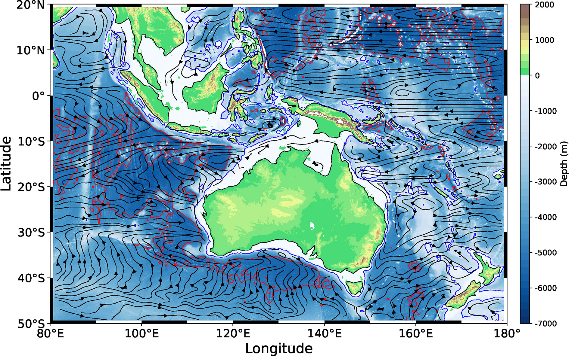
Figure 1 Topography of the Indo-Pacific Maritime Continent (shaded, unit in m) and mean horizontal currents averaged over the upper 100 m layer from SODA (black streamlines). Blue contour lines denote the 1000 m isobaths, and red contour lines denote the 5000 m isobaths.

Case 1: The geometry of Case 1 is shown in Figure 2. The western island partially overlaps with the middle and eastern islands in latitude, while the middle island and eastern island do not overlap with each other in latitude (Figure 2). In the original Godfrey’s island rule, the viscous effects of the interior ocean and the eastern boundary is ignored. But different from the single island, the frictional effects between the island channels for the multiple islands are considered in the present study. We integrate the wind stress and friction terms in Eq. (1), (2) along the closed curves C₀, C₁, and C₂, and get:

FIGURE 2

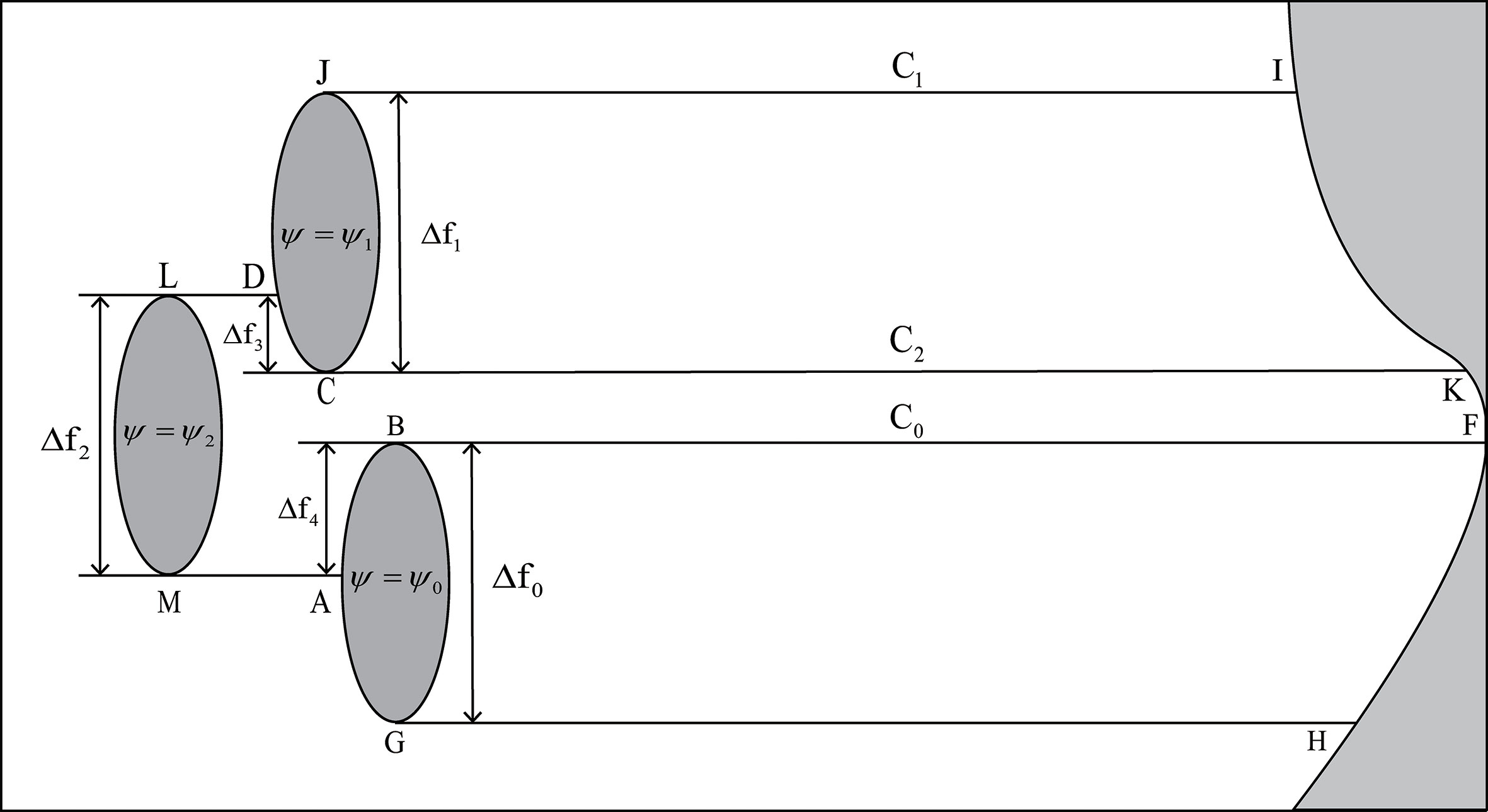
Figure 2 Map of islands and path of integration in Case 1.

$\begin{array}{ll}\Delta f_0{\psi }_0=-\underset{c_0}{\oint }\frac{\overrightarrow{\tau }}{{\rho }_0}·d\overrightarrow{l}+\underset{A}{\overset{B}{\int }}\overrightarrow{F}·d\overrightarrow{l},& (3)\end{array}$

$\begin{array}{ll}\Delta f_1{\psi }_1=-\underset{c_1}{\oint }\frac{\overrightarrow{\tau }}{{\rho }_0}·d\overrightarrow{l}+\underset{C}{\overset{D}{\int }}\overrightarrow{F}·d\overrightarrow{l},& (4)\end{array}$

$\begin{array}{ll}\Delta f_2{\psi }_2=-\underset{c_2}{\oint }\frac{\overrightarrow{\tau }}{{\rho }_0}·d\overrightarrow{l}-\underset{A}{\overset{B}{\int }}\overrightarrow{F}·d\overrightarrow{l}-\underset{C}{\overset{D}{\int }}\overrightarrow{F}·d\overrightarrow{l}+\Delta f_4{\psi }_0+\Delta f_3{\psi }_1.& (5)\end{array}$

Then,

$\begin{array}{ll}{\psi }_0={\psi }_{0,wind}+\frac{1}{\Delta f_0}\underset{A}{\overset{B}{\int }}\overrightarrow{F}·d\overrightarrow{l},& (6)\end{array}$

$\begin{array}{ll}{\psi }_1={\psi }_{1,wind}+\frac{1}{\Delta f_1}\underset{C}{\overset{D}{\int }}\overrightarrow{F}·d\overrightarrow{l},& (7)\end{array}$

$\begin{array}{ll}{\psi }_2={\psi }_{2,wind}-\frac{\Delta f_0-\Delta f_4}{\Delta f_2}·\frac{1}{\Delta f_0}\underset{A}{\overset{B}{\int }}\overrightarrow{F}·d\overrightarrow{l}-\frac{\Delta f_1-\Delta f_3}{\Delta f_2}·\frac{1}{\Delta f_1}\underset{C}{\overset{D}{\int }}\overrightarrow{F}·d\overrightarrow{l}.& (8)\end{array}$

Where Δf_i,i=1,2,3,4 denotes the difference of Coriolis parameters between the north and south latitudes, and $d\overrightarrow{l}$ represents the differential vector along the direction of the integral path. And the streamfunctions of the island without considering the friction effect are:

$\begin{array}{ll}{\psi }_{0,wind}=-\frac{1}{\Delta f_0}\underset{\oint }{}{c}_0\frac{\overrightarrow{\tau }}{{\rho }_0}d\overrightarrow{l},& (9)\end{array}$

$\begin{array}{ll}{\psi }_{1,wind}=-\frac{1}{\Delta f_1}\underset{\oint }{}{c}_1\frac{\overrightarrow{\tau }}{{\rho }_0}d\overrightarrow{l},& (10)\end{array}$

$\begin{array}{ll}{\psi }_{2,\text{wind}}=\frac{\Delta f_4}{\Delta f_2}{\psi }_{0,\text{wind}}+\frac{\Delta f_3}{\Delta f_2}{\psi }_{1,\text{wind}}-\frac{1}{\Delta f_2}\underset{\oint }{}{c}_2\frac{\overrightarrow{\tau }}{{\rho }_0}·d\overrightarrow{l}.& (11)\end{array}$

As shown in Figure 2, the integral path around the island is all along the western coastline of the island (similarly hereinafter). The path of the integral curve C₀ is denoted by FBGHF, the path of the integral curve C₁ is signified by IJCKI, the path of the integral curve C₂ is represented by KCDLMABFK, and the curves AB and CD stand for the right-hand side (RHS) boundaries of the island channel.

Case 2: In this case, latitudes of the western island partially overlaps with that of the middle and eastern islands, and latitudes of the middle island partially overlaps with that of the eastern island (Figure 3). By integrating Eqs. (1) and (2) along the closed curves C₀, C₁, and C₂, we get:

FIGURE 3

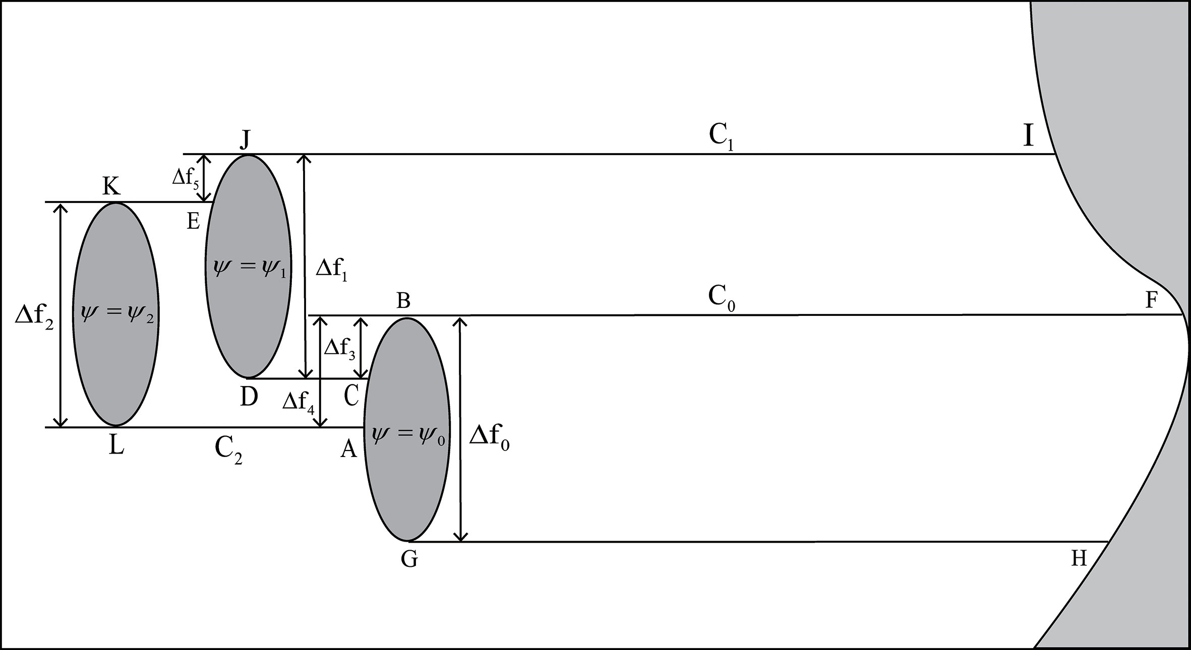
Figure 3 As in Figure 2 but for Case 2.

$\begin{array}{ll}{\psi }_0={\psi }_{0,\text{wind}}+\frac{1}{\Delta f_0}\underset{A}{\overset{B}{\int }}\overrightarrow{F}·d\overrightarrow{l},& (12)\end{array}$

$\begin{array}{ll}{\psi }_1={\psi }_{1,\text{wind}}+\frac{\Delta f_3}{\Delta f_1}·\frac{1}{\Delta f_0}\underset{A}{\overset{B}{\int }}\overrightarrow{F}·d\overrightarrow{l}+\frac{1}{\Delta f_1}(\underset{D}{\overset{E}{\int }}\overrightarrow{F}·d\overrightarrow{l}-\underset{C}{\overset{B}{\int }}\overrightarrow{F}·d\overrightarrow{l}),& (13)\end{array}$

$\begin{array}{ll}{\psi }_2={\psi }_{2,\text{wind}}+(\frac{\Delta f_4-\Delta f_0}{\Delta f_2}-\frac{\Delta f_3\Delta f_5}{\Delta f_1\Delta f_2})\frac{1}{\Delta f_0}\underset{A}{\overset{B}{\int }}\overrightarrow{F}·d\overrightarrow{l}-\frac{\Delta f_5}{\Delta f_1\Delta f_2}(\underset{D}{\overset{E}{\int }}\overrightarrow{F}·d\overrightarrow{l}-\underset{C}{\overset{B}{\int }}\overrightarrow{F}·d\overrightarrow{l}),& (14)\end{array}$

where,

$\begin{array}{ll}{\psi }_{0,\text{wind}}=-\frac{1}{\Delta f_0}\underset{\oint }{}{c}_0\frac{\overrightarrow{\tau }}{{\rho }_0}·d\overrightarrow{l},& (15)\end{array}$

$\begin{array}{ll}{\psi }_{1,\text{wind}}=\frac{\Delta f_3}{\Delta f_1}{\psi }_{0,\text{wind}}-\frac{1}{\Delta f_1}\underset{\oint }{}{c}_1\frac{\overrightarrow{\tau }}{{\rho }_0}·d\overrightarrow{l},& (16)\end{array}$

and

$\begin{array}{ll}{\psi }_{2,\text{wind}}=\frac{\Delta f_4}{\Delta f_2}{\psi }_{0,\text{wind}}-\frac{\Delta f_5}{\Delta f_2}{\psi }_{1,\text{wind}}-\frac{1}{\Delta f_2}\underset{\oint }{}{c}_2\frac{\overrightarrow{\tau }}{{\rho }_0}·d\overrightarrow{l},& (17)\end{array}$

represent streamfunctions when omitting the friction term, the path of the integral curve C₀ is specified by FBGHF, the path of the integral curve C₁ is represented by IJDCBFI, the path of the integral curve C₂ is denoted by IJEKLABFI, and the curves AB, CB, and DE stand for the RHS boundaries of the island channel.

Case 3: The western island contains the middle island in latitude and partially overlaps with the eastern island, and the middle island and the eastern island moderately overlap in latitude (Figure 4). Through integrating Eqs. (1) and (2) along the closed curves C₀, C₁, and C₂, we get:

FIGURE 4

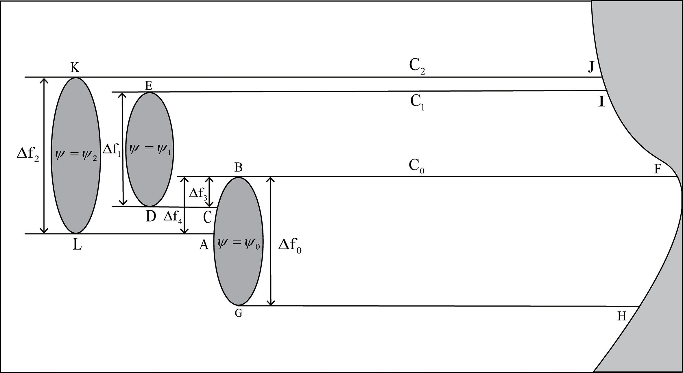
Figure 4 As in Figure 2 but for Case 3.

$\begin{array}{ll}{\psi }_0={\psi }_{0,\text{wind}}+\frac{1}{\Delta f_0}\underset{A}{\overset{B}{\int }}\overrightarrow{F}·d\overrightarrow{l},& (18)\end{array}$

$\begin{array}{ll}{\psi }_1={\psi }_{1,\text{wind}}+\frac{\Delta f_3}{\Delta f_1}·\frac{1}{\Delta f_0}\underset{A}{\overset{B}{\int }}\overrightarrow{F}·d\overrightarrow{l}+\frac{1}{\Delta f_1}(\underset{D}{\overset{E}{\int }}\overrightarrow{F}·d\overrightarrow{l}-\underset{C}{\overset{B}{\int }}\overrightarrow{F}·d\overrightarrow{l}),& (19)\end{array}$

$\begin{array}{ll}{\psi }_2={\psi }_{2,\text{wind}}-\frac{\Delta f_0-\Delta f_4}{\Delta f_2}·\frac{1}{\Delta f_0}\underset{A}{\overset{B}{\int }}\overrightarrow{F}·d\overrightarrow{l}.& (20)\end{array}$

In this formula,

$\begin{array}{ll}{\psi }_{0,\text{wind}}=-\frac{1}{\Delta f_0}\underset{\oint }{}{c}_0\frac{\overrightarrow{\tau }}{{\rho }_0}·d\overrightarrow{l},& (21)\end{array}$

$\begin{array}{ll}{\psi }_{2,\text{wind}}=\frac{\Delta f_4}{\Delta f_2}{\psi }_{0,\text{wind}}-\frac{1}{\Delta f_2}\underset{\oint }{}{c}_2\frac{\overrightarrow{\tau }}{{\rho }_0}·d\overrightarrow{l},& (22)\end{array}$

and

$\begin{array}{ll}{\psi }_{1,\text{wind}}=\frac{\Delta f_3}{\Delta f_1}{\psi }_{0,\text{wind}}-\frac{1}{\Delta f_1}\underset{\oint }{}{c}_1\frac{\overrightarrow{\tau }}{{\rho }_0}·d\overrightarrow{l}& (23)\end{array}$

denote streamfunctions when not considering friction. Further, the paths of the integral curve C₀, C₁, and C₂ are represented by FBGHF, IEDCBFI, and JKLABFJ, respectively, and the curves AB, CB, and DE denote the RHS boundary of the island channel.

Case 4: The western island partially overlaps with the middle island in meridional, the middle island partially overlaps with the eastern island in latitude, and the western island and eastern island do not overlap (Figure 5). By integrating Eqs. (1) and (2) along the closed curves C₀, C₁, and C₂, we have:

FIGURE 5

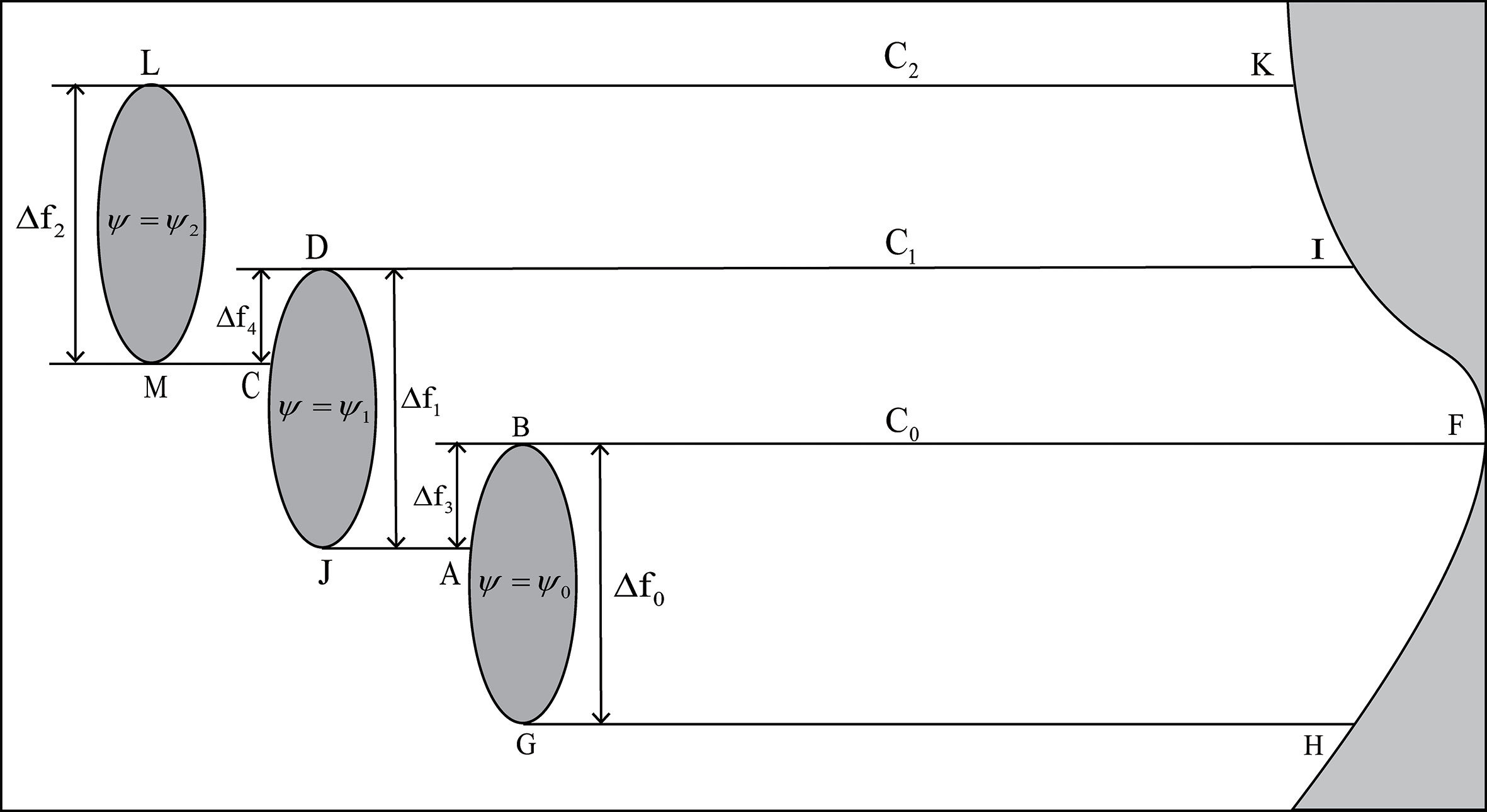
Figure 5 As in Figure 2 but for Case 4.

$\begin{array}{ll}{\psi }_0={\psi }_{0,\text{wind}}+\frac{1}{\Delta f_0}\underset{A}{\overset{B}{\int }}\overrightarrow{F}·d\overrightarrow{l},& (24)\end{array}$

$\begin{array}{ll}{\psi }_1={\psi }_{1,\text{wind}}-\frac{\Delta f_0-\Delta f_3}{\Delta f_1}·\frac{1}{\Delta f_0}\underset{A}{\overset{B}{\int }}\overrightarrow{F}·d\overrightarrow{l}+\frac{1}{\Delta f_1}\underset{C}{\overset{D}{\int }}\overrightarrow{F}·d\overrightarrow{l},& (25)\end{array}$

$\begin{array}{ll}{\psi }_2={\psi }_{2,\text{wind}}-\frac{\Delta f_4(\Delta f_0-\Delta f_3)}{\Delta f_1\Delta f_2}·\frac{1}{\Delta f_0}\underset{A}{\overset{B}{\int }}\overrightarrow{F}·d\overrightarrow{l}-\frac{\Delta f_1-\Delta f_4}{\Delta f_2}·\frac{1}{\Delta f_1}\underset{C}{\overset{D}{\int }}\overrightarrow{F}·d\overrightarrow{l}.& (26)\end{array}$

Where,

$\begin{array}{ll}{\psi }_{0,\text{wind}}=-\frac{1}{\Delta f_0}\underset{\oint }{}{c}_0\frac{\overrightarrow{\tau }}{{\rho }_0}·d\overrightarrow{l},& (27)\end{array}$

$\begin{array}{ll}{\psi }_{1,\text{wind}}=\frac{\Delta f_3}{\Delta f_1}{\psi }_{0,\text{wind}}-\frac{1}{\Delta f_1}\underset{c_1}{\oint }\frac{\overrightarrow{\tau }}{{\rho }_0}·d\overrightarrow{l},& (28)\end{array}$

and

$\begin{array}{ll}{\psi }_{2,\text{wind}}=\frac{\Delta f_4}{\Delta f_2}{\psi }_{1,\text{wind}}-\frac{1}{\Delta f_2}\underset{\oint }{}{c}_2\frac{\overrightarrow{\tau }}{{\rho }_0}·d\overrightarrow{l}& (29)\end{array}$

are streamfunctions when omitting the friction term. Additionally, the paths of the integral curves C₀, C₁, and C₂ in order are specified by FBGHF, IDJABFI, and KLMCDIK, and the curves AB and CD represent the RHS boundaries of the island channel.

Case 5: The setup of this case is the same as Case 1 but the width of M-A is reduced by 100 km.

2.3 Integral of lateral and bottom frictions

As shown in Section 2.2, the streamfunctions can be expressed as the sum of wind stress term and friction term. The wind stress term can be calculated from observed data of sea surface wind, but the friction force terms are not readily available, and the vorticity equations need to be solved firstly to establish the relationship between transport and friction term. Wajsowicz (1993) considered the situation of lateral and bottom frictions separately and modified the island rule. Yang et al. (2020) suggested that considering both the bottom and lateral friction may be of much importance. Hence in this study, we adopt the Munk-Stommel model (e.g., Stommel, 1948; Munk, 1950) following Yang et al. (2020), and the bottom and lateral frictions are substituted into Eqs. (1) and (2) at the same time:

$\begin{array}{ll}-f\frac{\partial \psi }{\partial x}=-\frac{1}{{\rho }_0}\frac{\partial p}{\partial x}-A_{\text{H}}(\frac{{\partial }^3\psi }{\partial x^2\partial y}+\frac{{\partial }^3\psi }{\partial y^3})+\frac{D_f}{Z}\frac{\partial \psi }{\partial y}+\frac{{\tau }^{(x)}}{{\rho }_0}\text{,}& (30)\end{array}$

$\begin{array}{ll}-f\frac{\partial \psi }{\partial y}=-\frac{1}{{\rho }_0}\frac{\partial p}{\partial y}+A_{\text{H}}(\frac{{\partial }^3\psi }{\partial x^3}+\frac{{\partial }^3\psi }{\partial x\partial y^2})-\frac{D_f}{Z}\frac{\partial \psi }{\partial x}+\frac{{\tau }^{(y)}}{{\rho }_0}\text{,}& (31)\end{array}$

Then the vorticity relation is given by:

$\begin{array}{ll}{A}_{\text{H}}(\frac{{\partial }^4\psi }{\partial x^4}+2\frac{{\partial }^4\psi }{\partial x^2\partial y^2}+\frac{{\partial }^4\psi }{\partial y^4})-A_{\text{S}}(\frac{{\partial }^2\psi }{\partial x^2}+\frac{{\partial }^2\psi }{\partial {\text{y}}^2})-\beta \frac{\partial \psi }{\partial x}+\nabla \times (\frac{\overrightarrow{\tau }}{{\rho }_0})=0\text{,}& (32)\end{array}$

where $A_{\text{S}}=\frac{D_f}{Z}$ and A_H represent the coefficients of the bottom friction and the lateral friction respectively, and $\beta =\frac{df}{dy}$ denotes the gradient of Coriolis parameter. We take into account a combination of friction coefficients and geometric/integral paths, although the bottom and lateral frictions used are simplified and idealized frictions and may have potential influences. This simplification may affect the exact value of ITF shipments, but does not change the main result in terms of ITF variability. Eq. (32) is a fourth-order partial differential equation, and it is difficult to obtain its analytical solution. Hence, the island channel is assumed to be a rectangular channel with width and length denoted by W and L (Figure 6). For the case of $\frac{W}{L}\ll 1$, we can rationally state that $\frac{\partial }{\partial x}\gg \frac{\partial }{\partial y}$, and thereby the vorticity equation is simplified to:

FIGURE 6

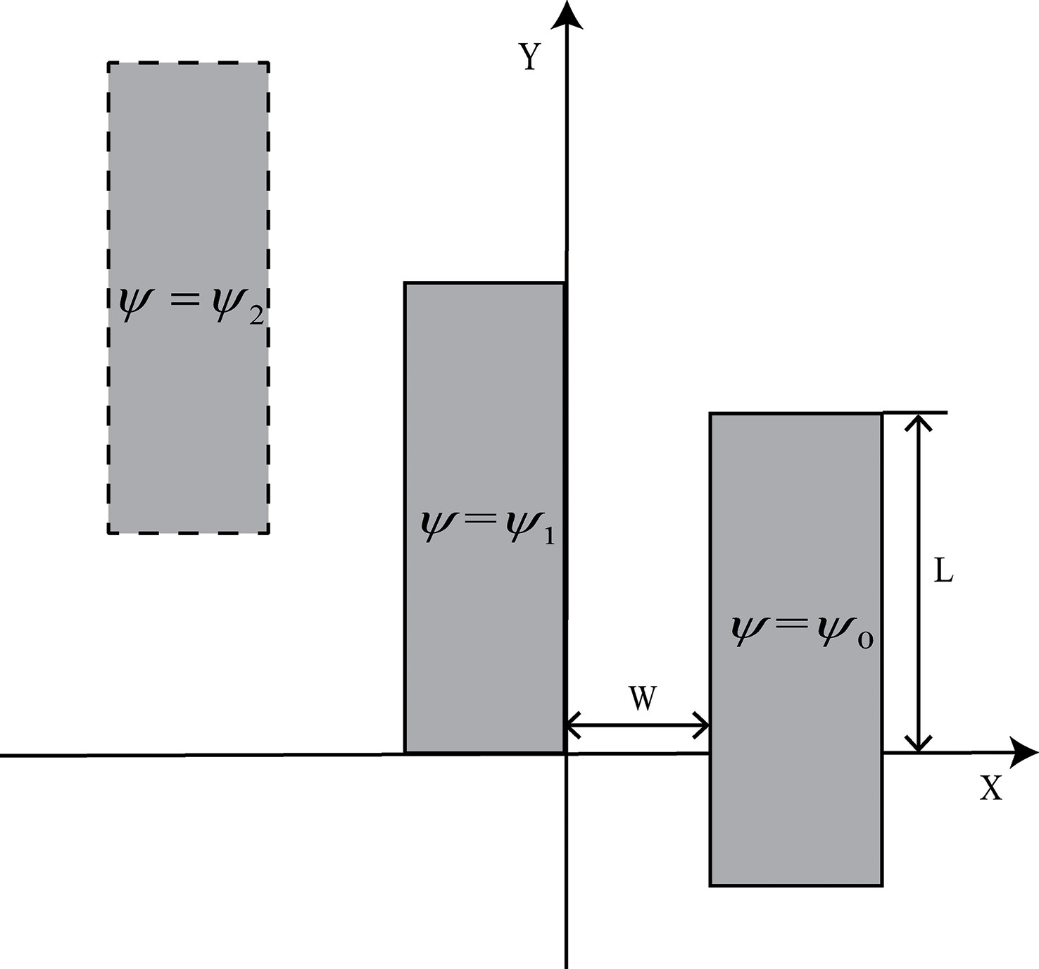
Figure 6 Schematic map of the passage between the two nearby islands.

$\begin{array}{ll}{A}_H\frac{{\partial }^4\psi }{\partial x^4}-A_S\frac{{\partial }^2\psi }{\partial x^2}-\beta \frac{\partial \psi }{\partial x}=-\nabla \times (\frac{\overrightarrow{\tau }}{{\rho }_0})& (33)\end{array}$

We first nondimensionalize Eq. (33), which is particularly important for the subsequent discussion of the contribution of bottom friction and lateral friction to transport and helps to diagnose the differences between the model and previous ones. We assume that there is a Sverdrup balance in the channel, then the last term on the left and the first term on the right of Eq. (33) are balanced. If U is the characteristic scale of horizontal velocity, W is the characteristic scale of horizontal length, and τ₀ is the characteristic scale of τ , then there is U=τ₀ρ₀⁻¹β⁻¹W⁻¹. If ψ is normalized by UW, we get the following formula:

$\begin{array}{ll}{(\frac{{\delta }_M}{W})}^3{\nabla }^4\psi -\frac{{\delta }_S}{W}{\nabla }^2\psi -{\psi }_x=-\nabla \times \overrightarrow{\tau }\text{,}& (34)\end{array}$

$${\delta }_M={(A_H/\beta )}^{1/3}\text{,}{\delta }_s = A_S/\beta \text{,}$$

where, δ_M is the Munk boundary layer thickness and δ_s corresponds to the Stommel boundary layer thickness. The lateral friction coefficient is set as A_H=10⁴ m² s⁻¹ (Wajsowicz, 1996), the bottom friction coefficient is set as $A_{\text{S}}= \frac{2}{3}\times {10}^{-5} {\text{s}}^{-1}$ (The water depth is taken as 300m) following Yang et al. (2020), and the gradient of Coriolis parameter is set as  β=1.62×10⁻¹¹ m⁻¹ s⁻¹ . Therefore, the Munk boundary layer is δ_M =85 km, the Stommel boundary layer is  δ_s = 412 km, and δ_M is less than δ_s. For simplification, friction is considered only when the strait width is less than the boundary layer thickness, and hence we choose different models according to the width of channel.

1) When 0<W≤δ_M<δ_s, both the bottom friction and lateral friction are considered and the model is similar to the Munk-Stommel model. Eq. (33) is then expressed as follows:

$\begin{array}{ll}\frac{{\partial }^4\psi }{\partial x^4}+a\frac{{\partial }^2\psi }{\partial x^2}+b\frac{\partial \psi }{\partial x}=d\text{here,}a=-\frac{A_S}{A_H} b=\frac{-\beta }{A_H} d=-\frac{1}{A_H}\nabla \times (\frac{\overrightarrow{\tau }}{{\rho }_0})\text{,}& (35)\end{array}$

with the following boundary conditions:

$$\psi (0\text{,}y)={\psi }_1\text{,}\psi (W\text{,}y)={\psi }_0\text{,}{(\frac{\partial \psi }{\partial x})}_{x=0}=0\text{,}{(\frac{\partial \psi }{\partial x})}_{x=W}=0$$

By introducing boundary conditions, we get the general solution of Eq. (35):

$\begin{array}{ll}\psi (x,y)=l_0+l_1{e}^{r_{1}x}+l_2{e}^{r_{2}x}+l_3{e}^{r_{3}x}+\frac{d}{b}x\text{,}& (36)\end{array}$

where, r₁, r₂ and r₃ represent the roots of the characteristic equation, l₀, l₁, l₂ and l₃ are constants. Please refer to the appendix for detailed derivation process.

Integrating the friction expression along the length and we have:

$\begin{array}{ll}\begin{array}{l}{{\displaystyle {\int }_O^L\overrightarrow{F}·d\overrightarrow{l}={\displaystyle {\int }_O^L[A_H(\frac{{\partial }^3\psi }{\partial x^3})}}}_{x=W}-A_s{(\frac{\partial \psi }{\partial x})}_{x=W}]dy\\ ={\displaystyle {\int }_O^L{A}_H}[{(\frac{{\partial }^3\psi }{\partial x})}_{x=W}+a{(\frac{\partial \psi }{\partial x})}_{x=W}]dy\\ =A_{H}L[{\displaystyle {\sum }_{i=1}^3{l}_i{r}_i}{e}^{r_{i}W}(r_i{2}^{}+a)+\frac{ad}{b}]\\ =m+n({\psi }_O-{\psi }_1)\end{array}& (37)\end{array}$

where

$$m=\frac{A_{H}Lad}{b}+\frac{A_{H}Ld}{b}{\displaystyle \sum _{i=1}^2{\displaystyle \sum _{i<j\le 3}{(-1)}^{i+j}\left\{(r_k{3}^{}+a{r}_k)(r_i-r_j)e^{r_{k}w}+[r_k(r_i{3}^{}-r_j{3}^{})-r_i{r}_j(1+W{r}_k)(r_i{2_{}}^{}-r_j{2}^{})+a{r}_k(r_i-r_j)]e^{{\text{(r}}_{\text{i}}{\text{+r}}_{\text{j}}\text{)W}}+r_k{3}^{}(r_i-r_j)e^{(r_i+r_2+r_3)W}\right\}/{\displaystyle \sum _{i=1}^2{\displaystyle \sum _{i<j\le 3}{(-1)}^{i+j+1}{r}_k(r_i+r_j}}}})(e^{r_i+r_j)W}-e^{rkW})$$

$n=\frac{A_{\text{H}}L{r}_1{r}_2{r}_3{\sum }_{i=1}^2{\sum }_{i<j\le 3}{(-1)}^{i+j}(r_i{2}^{}-r_j{2}^{})e^{(r_i+r_j)W}}{{\sum }_{i=1}^2{\sum }_{i<j\le 3}{(-1)}^{i+j+1}{r}_k(r_i-r_j)(e^{(r_i+r_j)W}-e^{r_{k}W})}$

$$\text{(here,}k={(-1)}^{j}i+j\text{)}$$

2) When δ_M<W≤δ_s, the bottom friction is considered and the lateral friction coefficient is zero, and in this circumstances, the model is similar to the Stommel model. Eq. (33) is expressed as follows:

$\begin{array}{ll}\frac{{\partial }^2\psi }{\partial x^2}+a\frac{\partial \psi }{\partial x}=b \text{(here}, a=\frac{\beta }{A_S}, b=\frac{1}{A_S}\nabla \times (\frac{\overrightarrow{\tau }}{{\rho }_0})\mathrm{),}& (38)\end{array}$

with the following boundary conditions:

ψ(0,y)=ψ₁,

$$\psi (W,y)={\psi }_0$$

By introducing boundary conditions, we get the general solution to Eq. (39):

$\begin{array}{ll}\psi (x,y)=l_0+l_1{e}^{r_{1}x}+\frac{b}{a}x\text{.}& (39)\end{array}$

Where, r₁ represents the root of the characteristic equation, l₀  and l₁ are constants. Please refer to the appendix for detailed derivation process.

Integrate the friction expression along the length; therefore, we have:

$\begin{array}{ll}\begin{array}{c}\underset{0}{\overset{L}{\int }}\overrightarrow{F}·d\overrightarrow{l}=-\underset{0}{\overset{L}{\int }}{A}_{\text{S}}{(\frac{\partial \psi }{\partial x})}_{x=W}dy\\ =-A_{S}L(l_1{r}_1{e}^{r_{1}W}+\frac{b}{a})\\ =m+n({\psi }_0-{\psi }_1)\end{array}\text{.}& (40)\end{array}$

In the formula, $m=\frac{A_{S}Lb}{a}(\frac{W{r}_1}{1-e^{-r_{1}W}}-1)$, $n=-\frac{A_{S}L{r}_1}{1-e^{-r_{1}W}}$.

3) When δ_M<δ_s<W, the bottom friction and lateral friction are not considered, so the integral of friction is zero.

2.4 Influence of geometry on channel transport

To examine the influence of geometry on the channel transport, we then estimate the transport ψ₀−ψ₂, i.e., the through flow in the channel between the western island and the eastern island, in the five cases. The monthly average wind speed data at 10 meters above the sea surface based on the CCMP (Cross-Calibrated Multi-Platform) are employed. The CCMP wind speed data spans from 2004 to 2006 with a spatial resolution of 0.25°×0.25°, and the sea surface wind stress is obtained by using the empirical formula. It should be noted that, previous studies have suggested that wind stress calculated by actual wind and relative wind might have an impact on ocean current simulations (e.g., Wu et al., 2012; Sun et al., 2021), but in order to contrast with the previous island rule, only actual wind is considered in this paper. The drag coefficient of wind stress has been investigated in numerous previous studies (e.g., Garratt, 1977; Powell et al., 2003). Here, we employ the empirical formula associated with the wind stress and drag coefficient following Yelland and Taylor (1996):

$\begin{array}{ll}\begin{array}{c}{\tau }_{\text{x}}={\rho }_{\text{a}}{C}_{\text{D}}\left|\overrightarrow{V}\right|u\\ {\tau }_{\text{y}}={\rho }_{\text{a}}{C}_{\text{D}}\left|\overrightarrow{V}\right|v\end{array}\text{.}& (41)\end{array}$

$\begin{array}{ll}{C}_{\text{D}}\times 1000=\{\begin{array}{c}0.29+\frac{3.1}{\left|\overrightarrow{V}\right|}+\frac{7.7}{{\left|\overrightarrow{V}\right|}^2}, 3m/s<\left|\overrightarrow{V}\right|<6m/s\\ 0.6+0.07\left|\overrightarrow{V}\right|, 6m/s<\left|\overrightarrow{V}\right|<26m/s\end{array}& (42)\end{array}$

where τ_x and τ_y represent the zonal and meridional wind stresses, ρ_a=1.29 kg m⁻³ is the air density, C_D denotes the drag coefficient, $\left|\overrightarrow{V}\right|$ is the modulus of the wind vector, and u and v are the components of the wind speed in the east-west and north-south directions, respectively. We assumed that the width of the channel is constant in each case. The width (W₂ ) of the channel between the western island and the middle island is set as 100km, the width (W₁) of the channel between the western island and the eastern island is set as 200km (this assumption is valid only when there is a channel between the two islands), and the climatological wind stress curl between channels is adopted.

Table 1 presents the latitude ranges of the islands and corresponding channel transports in the five cases. Note that the total transport in Case 1 equals to the channel transport through the section M-A, in Case 2 equals to the channel transport through the section L-A, in Case 3 equals to the channel transport through the section L-A, and in Case 4 equals to the channel transport through the section M-C plus J-A. As shown in Table 1, the channel transport decreases from 14.47 Sv in Case 1 to 8.70 Sv in Case 2. The difference of islands’ setup between Case 1 and Case 2 is the latitude of the middle island, which leads to changes of channel friction and integral paths. The main changes of geometry in Case 3 from Case 2 are a reduction in length and southward shift of the middle island (Table 1 and Figure 4). As a result, the western island streamfunction in Case 3 would be no longer affected by the friction of the western boundary of the middle island, and the transport rises to 10.12 Sv. In Case 4, the western island is shifted to the north by 6° relative to Case 3 and does not coincide with the eastern island in latitude. Although the geometry changes in case 4 lead to an increase of friction, the streamfunction of the western island in Case 4 is affected by the middle island compared to Case 3, in which the transport is further increased to 12.75 Sv. The Case 5 is similar to Case 1. Compared with Case 1, the latitude range of islands in Case 5 remains unchanged, but the width of the channel between the middle and eastern islands is reduced by 100 km. As a result, the transport is decreased from 14.47 Sv in Case 1 to 9.02 Sv in Case 5, due to the narrowing down of the channel and a larger contribution of bottom friction. To summarize, the above comparison indicates that the channel’s transport is very sensitive to geometry through the effect of friction and integral paths.

TABLE 1

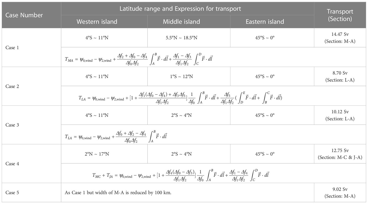
Table 1 Islands setup and corresponding channel transports in the five cases.

3 ITF transport estimate with inclusion of North Pacific winds

3.1 ITF transport estimate

The Indonesian Seas where the ITF passes by have a very complex geometry and bathymetry. Here we optimize the integral path for simplification. Figure 7 demonstrates the climatological sea surface winds in the Pacific Ocean and the integral path we used. Arrows represent the climatological winds from the CCMP product. The distribution of the three islands and the streamfunctions are represented by the idealized Case 1 discussed in Section 2.2. The Makassar Strait is the main inflow channel for the ITF (Wajsowicz, 1996; Susanto and Gordon, 2005; Vranes and Gordon, 2005), accounting for 75%-80% of the ITF water transport (Gordon et al., 2008; Li et al., 2018; Gordon et al., 2019). Case 1 is an idealized geometry, and it needs to be adjusted according to the actual geometry in the estimation of ITF. The channel’s width W₁ shown in Figure 7 includes the width of the Makassar Strait and the Lifamatola Strait. Although the Lifamatola Strait is also an entrance to the ITF, its contribution to the ITF is small compared to the overall transport and its width is negligible compared to the Makassar Strait. Therefore, we only take into account the width of the Makassar Strait. Suppose that the width and length of the Makassar Strait are represented by W₁ and L₁, and the width and length of the Mindoro Strait are denoted by W₂ and L₂, respectively. Then the transports through the Mindoro Strait and Makassar Strait specified by T₁ and T₂ are:

FIGURE 7

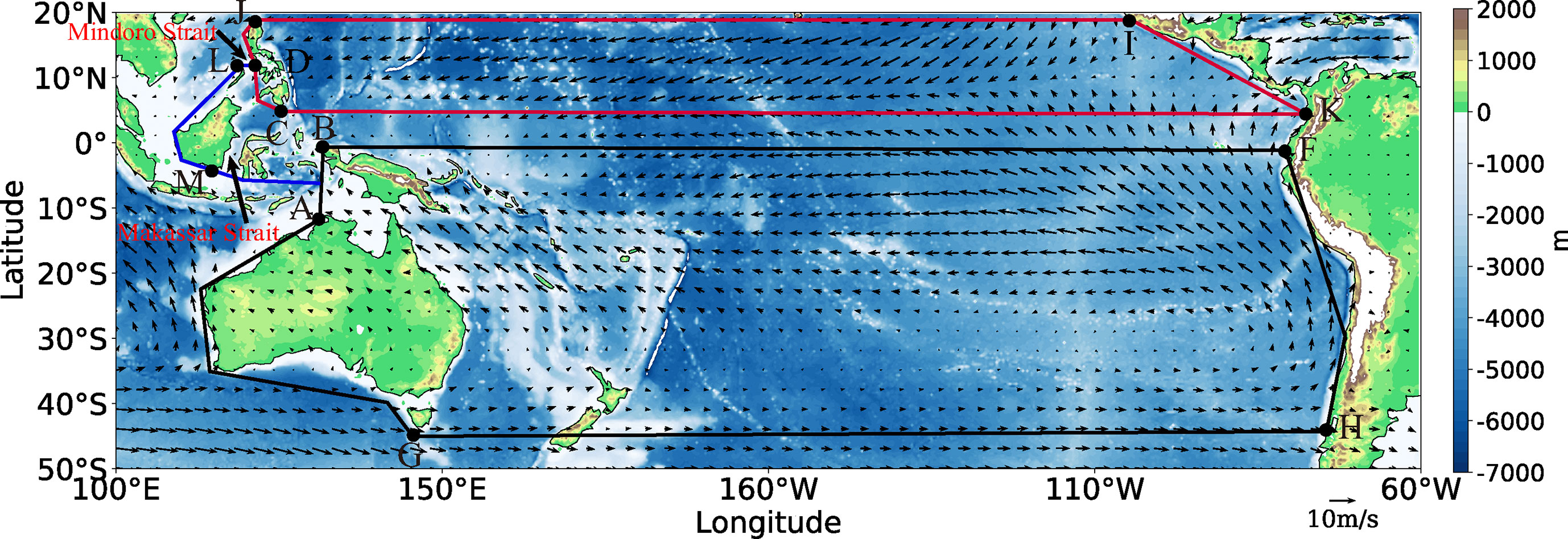
Figure 7 Integral paths (red, blue and black lines) and climatological sea surface winds (vectors). Color shading shows the topography (unit in m).

$\begin{array}{ll}{T}_1={\psi }_1-{\psi }_2={\psi }_{1,\text{wind}}-{\psi }_{2,\text{wind}}+R_1{m}_1+R_2{m}_2+R_1{n}_1({\psi }_0-{\psi }_2)+R_2{n}_2({\psi }_1-{\psi }_2),& (43)\end{array}$

$\begin{array}{ll}{T}_2={\psi }_0-{\psi }_2={\psi }_{0,\text{wind}}-{\psi }_{2,\text{wind}}+R_3{m}_1+R_4{m}_2+R_3{n}_1({\psi }_0-{\psi }_2)+R_4{n}_2({\psi }_1-{\psi }_2)\text{.}& (44)\end{array}$

$$R_1=\frac{\Delta f_0-\Delta f_4}{\Delta f_0\Delta f_2}, R_2=\frac{\Delta f_1-\Delta f_3+\Delta f_2}{\Delta f_1\Delta f_2}, R_3=\frac{\Delta f_0-\Delta f_4+\Delta f_2}{\Delta f_0\Delta f_2}, R_4=\frac{\Delta f_1-\Delta f_3}{\Delta f_1\Delta f_2}.$$

m₁ and n₁ are formally the same as the expression m and n in Section 2.3, except that L₁ and W₁ replace L and W in the formula. Same thing with m₂ and n₂ .

By simultaneous solving the relations in Eq. (43) and Eq. (44), the transport of the Makassar Strait is obtained as:

$\begin{array}{ll}{T}_2=\frac{R_4{n}_2({\psi }_{1,\text{wind}}-{\psi }_{2,\text{wind}}+R_1{m}_1+R_2{m}_2)+(1-R_2{n}_2)({\psi }_{0,\text{wind}}-{\psi }_{2,\text{wind}}+R_3{m}_1+R_4{m}_2)}{1-R_2{n}_2-R_3{n}_1+R_2{R}_3{n}_1{n}_2-R_1{R}_4{n}_1{n}_2}& \text{. (45)}\end{array}$

To calculate the ITF transports over a long period of time, we extend the time span of the monthly sea surface wind product of CCMP to 1988-2016. The geometry data of the Makassar Strait and Mindoro Strait are given by: W₁=200km, L₁=1200km, W₂=100km, L₂=700km, and the average wind stress curl between channels is set as $rot(\stackrel{\rightharpoonup }{\tau })=-5.42\times {10}^{-8}{\text{ N m}}^{\mathrm{-3}}$. Because δ_M<W₁≤δ_s, the width of the channel is much larger than the Munk boundary layer thickness, and the lateral friction is not included in the calculation, so the Stommel model is adopted. The time series of ITF from 1988 to 2016 can be obtained by inserting parameters and wind stress data into the Eq (45).

Figure 8A illustrates the yearly mean transport of ITF from the INSTANT observations and that calculated with island rule during 2004–2006. The INSTANT program deployed 11 moorings in the major inflow and outflow passages of the ITF during 2004–2006, and the total transport through three passages (Lombok Strait, Ombai Strait, and Timor Passage) during the INSTANT period was 15.0 Sv (Sprintall et al., 2009). As shown in Figure 8A, the ITF transport predicted by G1989 and Y2020 are smaller than the observed value, and the ITF transport derived from the multiple islands rule of this study has the smallest difference from the observations. Figure 8B compares the 13-month running mean ITF transport anomalies during 2004–2006 and the INSTANT observations. The INSTANT observations show that the ITF transport had a peak in 2005 and was relatively weaker in 2004 and 2006. As shown in Figure 8B, the ITF transport from the triple island rule theory has a significant correlation coefficient of about 0.9 with the INSTANT ITF transport, while the correlation coefficient between original island rule transport and the INSTANT ITF transport is only 0.25, implying that the multiple islands rule of this study is able to infer a more reasonable time series and shows significant improvement in estimating the ITF transport comparing with the original island rule theory.

FIGURE 8

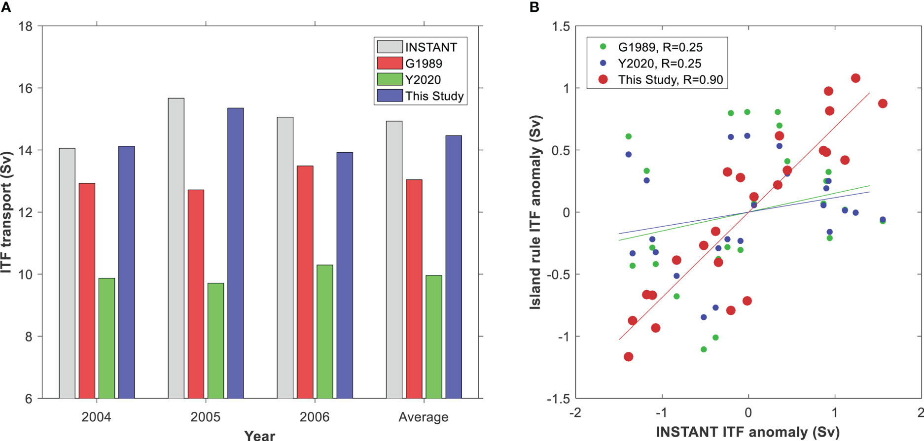
Figure 8 (A) Annual mean ITF transports calculated by the island rule theory and measured by the INSTANT program. (B) Comparison between 13-month running mean anomalies of ITF transport from island rule theory and the INSTANT observations. “R” in the right panel denotes the correlation coefficients between island rule ITF and INSTANT ITF transport.

To further verify the multiple islands rule in a longer time period, we plot in Figure 9 the yearly transports during 1988–2016 from G1989, Y2020 and the present study, with a 6-month running mean of the data in advance. The annual and monthly average ITF transport by INSTANT during 2004–2006 and the annual mean ITF transport calculated using the MITF velocity are also added to the picture. Note that the monthly average has been subjected to a 13-month running mean to remove seasonal signals. The MITF program deployed two moorings in the Makassar Strait, on which two acoustic Doppler current profilers (ADCPs) measured the Makassar throughflow from surface to the 680 m sill depth (Gordon et al., 2003; Gordon et al., 2019). The time span of MITF velocity dataset is from November 2006 to December 2016 (Only eight months of data in 2017 and hence are not used). By splicing it with the INSTANT observation dataset, the time span is expanded to January 2004 – December 2016, and it was pre-processed into a time interval of one day. Since MITF program only conducted mooring observation in the Makassar Strait and not for the entire ITF, we use the INSTANT time series to correct the MITF transport through a formula to get a MITF-based transport of the total ITF.

FIGURE 9

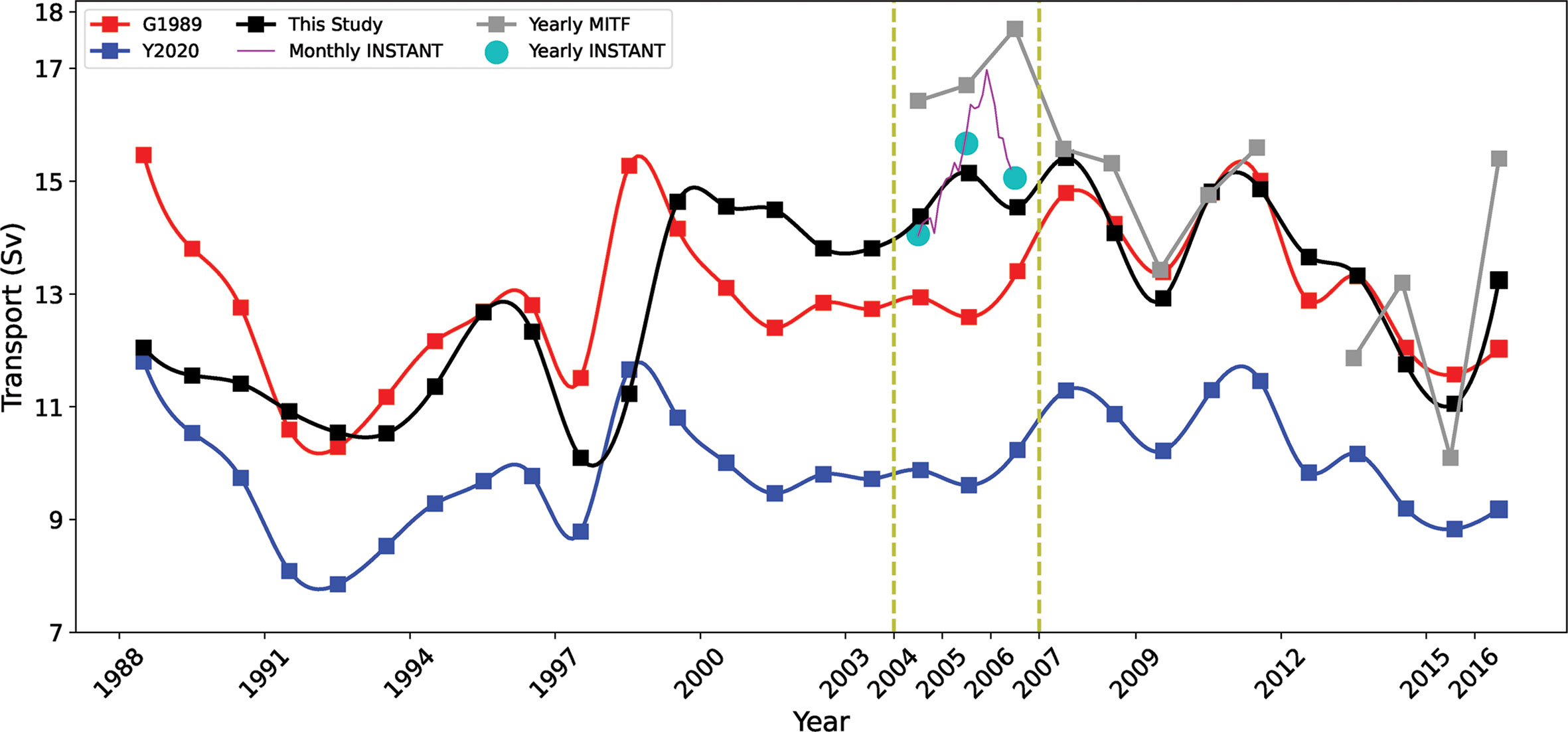
Figure 9 Yearly ITF transport during 1988-2016 derived from G1989 (red), Y2020 (blue) and the solution of this study (black). Yearly and monthly INSTANT observations during 2004-2006 (cyan and magenta respectively) and yearly MITF transport during 2004-2016 (gray) are also shown for comparison.

First of all, we averaged the single point velocity measured by ADCP in the vertical direction to obtain the average velocity of each day, and then averaged to get the average speed of the whole time period. The ratio of the two was multiplied by the average flow of INSTANT to obtain the MITF transport, and the corresponding expression is $\text{MITF=}{\stackrel{}{\text{V}}}_{\text{vertical}}/{\stackrel{}{V}}_{\text{time}}\times 15$, ${\stackrel{}{V}}_{\text{vertical}}$ represents the vertical average of the horizonal velocity, the number 15 represents the average ITF transport during the INSTANT period, and ${\stackrel{}{V}}_{\text{time}}$ represents the average over the time dimension of ${\stackrel{}{V}}_{\text{vertical}}$.

As shown in Figure 9, the average transports from G1989, Y2020 and the present study are 13.03 ± 3.30 Sv, 9.94 ± 2.52 Sv, and 13.00 ± 3.94 Sv during 1988–2016, respectively. Observations show that the ITF transport during 2004–2015 was about 15.64 Sv (Li et al., 2018), and for comparison, the average transports during 2004–2015 from G1989, Y2020 and the present study are 13.60 ± 0.87 Sv, 10.38 ± 0.51 Sv and 14.10 ± 1.02 Sv, respectively. Hence, in general, the multiple islands rule of this study predicts a reasonable mean transport that is consistent with observations.

Both the G1989 and the multiple islands rule predict a reasonable mean transport of about 13.03 and 13.00 Sv, but the G1989 transport show significant differences in interannual peaks and valleys comparing with observations. For example, geostrophic calculations indicate that the ITF in about 1988–1989 was smaller than that of the 1990s and 2000s (Liu et al., 2015), but in contrast, the transport from G1989 and Y2020’s island rule is greater in 1988 than that in 1990s and 2000s (Figure 9).

We then calculated the average errors of the three (G1989, Y2020, and this study) time series and their correlation coefficients with the MITF time series. Here, the average error is defined as the average of the difference between a time series and the MITF time series. The average errors of the former two (G1989 and Y2020) are 1.32 Sv and 4.48 Sv, respectively, which are much greater than that of the present study that is only 0.87 Sv. The correlation coefficient between the G1989 (Y2020) time series and the MITF is both 0.37 (0.37), while the time series from the multiple island rule and the MITF has a correlation coefficient of 0.81. Therefore, the comparison implies that the multiple islands rule might be improved from previous studies of island rule theory. It should be noted that, since the time series from the island rule shown in Figure 9 were calculated using the same wind stress data set, the significant differences between them should be attributed to from the optimizing of the fraction and path of integration related to the geometry.

As we mentioned, Pratt and Pedlosky (1998) examined the role of lateral friction in the island rule theory, and pointed out that lateral friction is an important factor in the overestimation of ITF in the original island rule. But it seems that the major straits (e.g., Makassar Strait) of the ITF passing by have a width greater than the thickness of Munk boundary layer except a few narrow passages, and the lateral friction from these narrow passages may have limited influence on the overall transport. As an alternative, the inter-channel bottom friction, which can significantly reduce the estimate of ITF, may play an important role. As we tested, the ITF transport can reach 27.6 Sv, which is obviously unreasonable, if the inter-channel bottom friction dissipation in the Indonesian sea is not taken into account.

3.2 The influence of including North Pacific winds

The island rule reflects the relationship between the ITF transport and the Pacific wind field. Previous studies suggest that the decadal variability of ITF is related to the North Pacific trade winds and the ITF is primarily drawn from North Pacific thermocline waters (e.g., Li et al., 2018; Li et al., 2020). The North Pacific trade winds has significant impact on the Northern Equatorial Current (NEC) bifurcation latitude and Mindanao Current (MC) and hence the ITF (e.g., Hu et al., 2016; Hu et al., 2020; Hu et al., 2021). One of changes in the present multiple islands rule from previous theories is the inclusion of wind stress of northern Pacific Ocean in the path of integration, and this change might play an important role in producing a better estimate of ITF transport.

The original island rule suggests that the major forcing for the ITF transport (T=ψ_0, wind ) is the wind field in the eastern ocean of Australia-PNG. In other words, the magnitude and variability of the ITF would depend only on the zonal wind stress across the Pacific at the northernmost and southernmost latitudes of Australia-PNG and the alongshore wind stress along the western coasts of Australia and South America (Wajsowicz, 1993). The wind in the southern hemisphere definitely plays an important role in determining the ITF transport. However, the upstream of ITF include not only the southern Pacific ocean circulation, but also the major currents in the norther Pacific Ocean which are mainly controlled by wind forcing from the norther Pacific Ocean. For example, the MC, which comes from the wind-driven current the NEC (McCreary and Lu, 1994), is an important source of the ITF but controlled by the northern Pacific winds (e.g., Hu et al., 2016; Hu et al., 2021). Godfrey et al. (1993) proposed that the ITF is supplied by the MC, and Gordon (1995) suggested that the ITF mainly originates from the North Pacific Ocean, and the seawater from the MC is mainly transported southward through Makassar Strait.

In addition, the northern Pacific Ocean also feeds the ITF through the South China Sea (e.g., Gordon et al., 2019). The Kuroshio flows into the South China Sea through the Luzon Strait in winter under the influence of the Northeast monsoon (Wyrtki, 1961). Lebedev and Yaremchuk (2000) pointed out that the inflow of the Luzon Strait contributes significantly to the ITF, the seawater from the North Pacific flows into the South China Sea through the Luzon Strait, and part of it flows south through the Mindoro Strait, and then farther on until it joins a powerful current, which can be seen as an extension of the MC. So, changes of the North Pacific wind field cause the response of MC and Kuroshio and further affect the ITF.

As can be seen from Eq. (45), considering that the ITF volume transport of multiple islands is determined by the wind stress field in the South Pacific (0°-45°S) and the North Pacific (0°-20°N), the transport value includes the flow through Mindoro Strait (i.e., T=ψ_1, wind−ψ_2, wind, with a source of the South China Sea) and Makassar Strait (i.e., T=ψ_0, wind−ψ_2, wind , with a source of the MC). So, the optimizing of the path of integration related to the geometry (i.e., including the northern Paicific Ocean) expectedly acts to improve the ITF estimates.

4 Sensitivity to boundary layer thickness and channel size

In the case of multiple islands, several factors, including bottom and lateral friction, channel width and length, are able to influence the estimated throughflow. The frictional boundary layer thickness is a monotonically increasing function of the frictional coefficient. To test the sensitivity of ITF transport to frictional coefficient and channel size, we examined the response of ITF transport from the multiple island rule to these factors. For simplification, we assume that the frictional coefficient can be represented by the boundary layer thickness in exploring the relationship between frictional coefficients and ITF transport.

Figure 10A shows the relationship between ITF transport and Stommel boundary layer thickness when the channel’s width is 200 km. It can be seen from the graph that the transport decreases with the increase of δ_S , but the decreasing rate gradually reduces. When the channel’s width is set to 50 km, Munk-type friction is also taken into account, and the flow decreased to varying degrees with the increase of δ_S and δ_M (Figure 10B). The contribution of the two kinds of friction is different. When the passage is relatively narrow, the Munk type friction dominates and the blockage of the current is stronger. It is interesting that, with the increase of Munk and Stommel boundary layer thickness, the lateral friction’s blocking effect on the ocean current is enhanced, while the bottom friction’s blocking effect on the ocean current is weakened, which is different from the conclusion when the passage is wider.

FIGURE 10

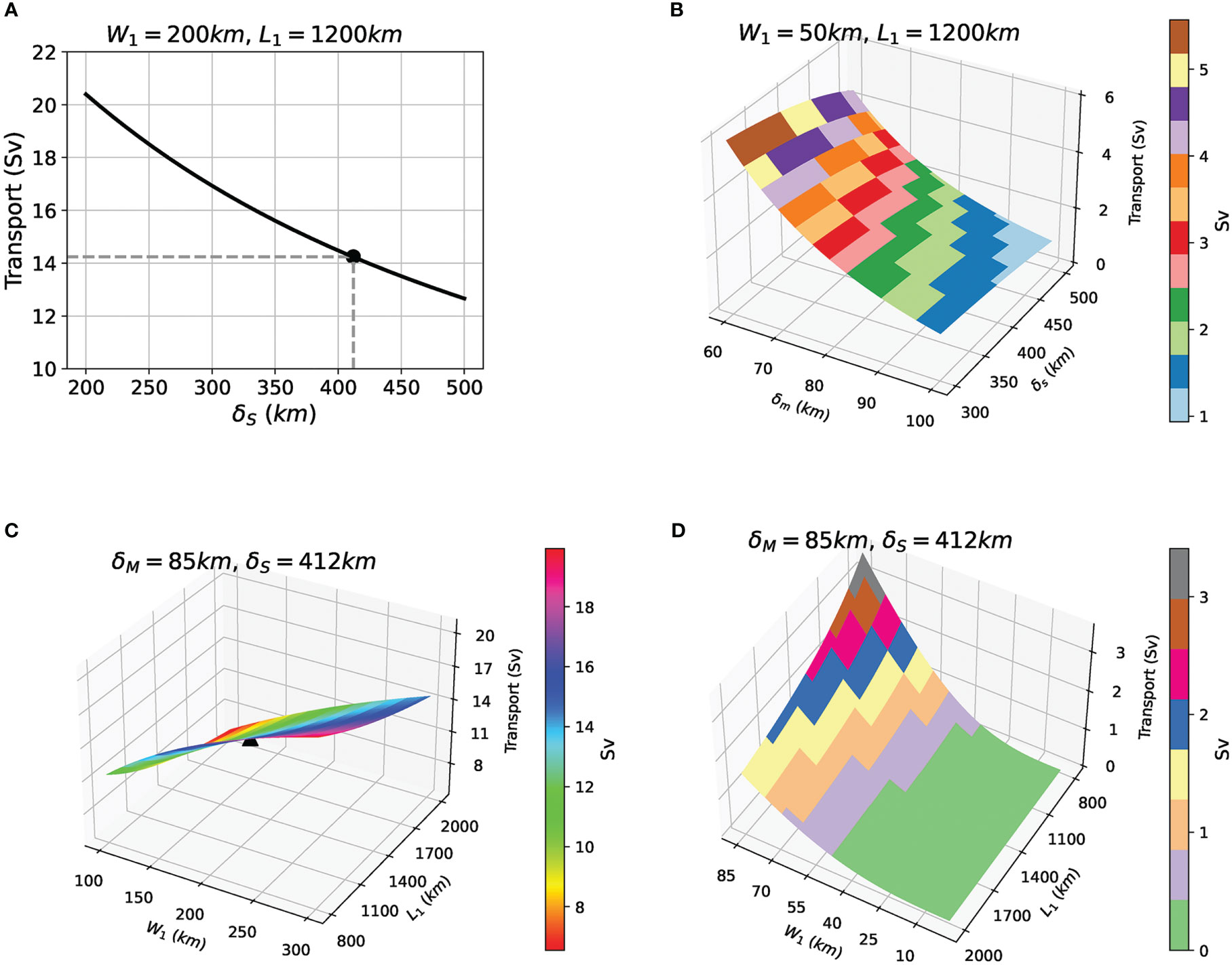
Figure 10 The idealized ITF transport as a function of various factors: thickness of Stommel boundary layer (A), thickness of both Munk and Stommel boundary layers (B), and channel size (C, D). The horizontal coordinates corresponding to the dot marks in (A) and the triangular marks in (C) are the parameters used in the estimation of ITF in this study.

We plot the derived ITF transport as a function of the channel’s width and length in the bottom panels of Figure 10. When δ_M<W₁≤δ_s , there is only bottom friction, ITF transport increases with the increase of channel’s width, and the growth rate gradually increases (Figure 10C). When 0<W₁≤δ_M<δ_s , both bottom friction and lateral friction play a role and the ITF transport still increases with the increase of channel’s width, but the rate of increase is accelerated (Figure 10D).

The reason why the rate of change is inconsistent is that when the channel is relatively narrow (less than δ_M ), the dominant lateral friction nonlinearity decreases rapidly with the increase of the channel’s width, and when the critical width (δ_M ) is reached, the lateral friction decreases to zero. When the width continues to increase, the current is completely controlled by the bottom friction, and the bottom friction obstructs the current more and more until the current rate changes stabilize. In contrast, the ITF transport is generally decreasing with an increasing of the channel’s length, which is not affected by the thickness of the boundary layer, and the rate of decrease gradually reduces (Figures 10C, D).

5 Discussion and conclusions

In this study, the island rule theory in the case of complex geometry with multiple islands referring to the Indo-Pacific Maritime Continent is investigated based on Godfrey’s island rule theory. To this end, the horizontal momentum equations were vertically integrated, the streamfunctions of islands under five cases with different geometry were calculated, and the transport through the channels was predicted. By comparing the transport in the five cases, we find that the geometry has a substantial influence on the transport of throughflow, due to changes in bottom and lateral friction and integral path associated with the geometry. The transport of the throughflow is negatively correlated with the frictional boundary layer thickness and channel length, but positively correlated with channel width, and the flow varies at different rates in different cases.

The ITF transport is estimated using this multiple islands rule with yearly wind stress data. During 2004-2006, the derived ITF transport is about 14.5 Sv, which is close to the observed ITF transport from INSTANT in the same duration (about 15.0 Sv). We compared the yearly ITF transport during 1988-2016 with that using G1989 and Y2020, and find that the multiple islands rule in this study is able to infer an improved estimate of ITF transport time series in terms of mean value and interannual variability. The ITF transport derived from the multiple islands rule is 13.00 ± 3.94 Sv, which is very close to direct observations. In addition, the island rule theory is applicable for low-frequency variability on which time scale the ITF adjustment to basin scale wind forcing is basically finished, so the theory is also applicable for variability of lower frequency like decadal variability.

Through a series of comparison between the multiple island rule, previous studies and observations, and sensitivity experiments, we suggest that the optimizing of the fraction and path of integration related to the geometry makes the multiple island rule be able to produce a time series of ITF transport that is in well agreement with observations. The comparison indicates that it is possible to produce a long time series of ITF transport from wind products using the multiple island rule, which is of much importance in monitoring the ITF and understanding the ocean circulation and climate system. It is worth mentioning that this study may have a potential value to the estimation of paleo-ITF transport.

Previous studies suggest that changes, including closures, opening and widening of the Indonesian seaway have happened in history (e.g., Kuhnt et al., 2013). The spatial features of the Indonesian straits might be similar with the paleo-geometry, hence the triple island rule theory is expected to be a good tool to estimate the paleo-ITF transport.

However, there is still room for further improvement in the multiple islands rule theory. For instance, in solving the vorticity equation, we assume that the width of the channel is much smaller than the length of the channel for simplification, and the problem has been not solved in the current investigation. In addition, time dependence may be important but is not explored here. In the near future, the theory might be further improved by adding the baroclinic term, time term, and other aspects.

Data availability statement

The original contributions presented in the study are included in the article/supplementary material. Further inquiries can be directed to the corresponding author.

Author contributions

SH designed the study. WS and SH conducted the analysis and wrote the initial version of the paper. All authors contributed to the article and approved the submitted version.

Funding

This study was supported by the Interdisciplinary Innovation Team of Chinese Academy of Sciences (JCTD-2020-12), the Strategic Priority Research Program of Chinese Academy of Sciences (No. XDB42010403), Shandong Provincial Natural Science Foundation (Grant ZR2020JQ18), the Laoshan Laboratory (No. 2022LSL010304), the Youth Innovation Promotion Association of Chinese Academy of Sciences (No. Y2022066), and the National Natural Science Foundation of China (Grants 42022040 and 91858101).

Acknowledgments

The SODA dataset is distributed by the International Pacific Research Center at the University of Hawaii at Mānoa: http://apdrc.soest.hawaii.edu/index.php (accessed 16 November 2022). The CCMP dataset was downloaded from https://www.remss.com/measurements/ccmp (accessed 16 November 2022). The ETOPO1 dataset can be found at https://www.ngdc.noaa.gov/mgg/global/global.html (accessed 16 November 2022). The MITF dataset was downloaded from https://academiccommons.columbia.edu/doi/10.7916/d8-p78a-zm51 (accessed 16 November 2022).

Conflict of interest

The authors declare that the research was conducted in the absence of any commercial or financial relationships that could be construed as a potential conflict of interest.

Publisher’s note

All claims expressed in this article are solely those of the authors and do not necessarily represent those of their affiliated organizations, or those of the publisher, the editors and the reviewers. Any product that may be evaluated in this article, or claim that may be made by its manufacturer, is not guaranteed or endorsed by the publisher.

References

Cai W. (2006). Antarctic Ozone depletion causes an intensification of the southern ocean super-gyre circulation. Geophysical Res. Lett. 33 (3), L03712–. doi: 10.1029/2005gl024911

CrossRef Full Text | Google Scholar

Deiters U. K. (2002). Calculation of densities from cubic equations of state. Aiche J. 48 (4), 882–6. doi: 10.1002/aic.690480421

CrossRef Full Text | Google Scholar

England M., Huang F. (2005). On the interannual variability of the Indonesian throughflow and its linkage with ENSO. J. Climate. 18 (9), 1435–1444. doi: 10.1175/JCLI3322.1

CrossRef Full Text | Google Scholar

Feng M., Böning C., Biastoch A., Behrens E., Weller E., Masumoto Y. (2011). The reversal of the multi-decadal trends of the equatorial pacific easterly winds, and the Indonesian throughflow and leeuwin current transports. Geophysical Res. Lett. 38 (11), L11604. doi: 10.1029/2011gl047291

CrossRef Full Text | Google Scholar

Feng M., Zhang N., Liu Q., Wijffels S. (2018). The Indonesian throughflow, its variability and centennial change. Geosci. Letters. 5 (1), 3. doi: 10.1186/s40562-018-0102-2

CrossRef Full Text | Google Scholar

Firing E., Qiu B., Miao W. (1999). Time-dependent island rule and its application to the time-varying north Hawaiian ridge current. J. Phys. Oceanography 29 (10), 2671–2688. doi: 10.1175/1520-0485(1999)029<2671:tdirai>2.0.co;2

CrossRef Full Text | Google Scholar

Forget G., Ferreira D. (2019). Global ocean heat transport dominated by heat export from the tropical pacific. Nat. Geoscience. 12, 351–354. doi: 10.1038/s41561-019-0333-7

CrossRef Full Text | Google Scholar

Garratt J. R. (1977). Review of drag coefficients over oceans and continents. Monthly Weather Review. 105 (7), 915–929. doi: 10.1175/1520-0493(1977)105<0915:RODCOO>2.0.CO;2

CrossRef Full Text | Google Scholar

Godfrey J. S. (1989). A sverdrup model of the depth-integrated flow for the world ocean allowing for island circulations. Geophysical Astrophysical Fluid Dynamics. 45 (1-2), 89–112. doi: 10.1080/03091928908208894

CrossRef Full Text | Google Scholar

Godfrey J. S. (1996). The effect of the Indonesian throughflow on ocean circulation and heat exchange with the atmosphere: A review. J. Geophysical Research: Oceans 101 (C5), 12217–12237. doi: 10.1029/95jc03860

CrossRef Full Text | Google Scholar

Godfrey J. S., Wilkin J., Hirst A. C. (1993). Why does the Indonesian throughflow appear to originate from the north pacific? J. Phys. Oceanography. 23 (6), 1087–1098. doi: 10.1175/1520-0485(1993)023<1087:wdtita>2.0.co;2

CrossRef Full Text | Google Scholar

Gordon A. L. (1986). Interocean exchange of thermocline water. J. Geophysical Res. 91 (C4), 5037–5046. doi: 10.1029/jc091ic04p05037

CrossRef Full Text | Google Scholar

Gordon A. L. (1995). When is appearance reality? a comment on why does the Indonesian throughflow appear to originate from the north pacific. J. Phys. oceanography. 25 (6), 1560–1567. doi: 10.1175/1520-0485(1995)025<1560:wiarac>2.0.co;2

CrossRef Full Text | Google Scholar

Gordon A. L. (2001). “Interocean exchange,” in Int. geophysics, vol. 77. (Acad. Press), 303–314. doi: 10.1016/S0074-6142(01)80125-X

CrossRef Full Text | Google Scholar

Gordon A. L., Fine R. A. (1996). Pathways of water between the pacific and Indian oceans in the Indonesian seas. Nature 379 (6561), 146–149. doi: 10.1038/379146a0

CrossRef Full Text | Google Scholar

Gordon A. L., Giulivi C. F., Ilahude A. G. (2003). Deep topographic barriers within the Indonesian seas. Deep Sea Res. Part II: Topical Stud. Oceanography. 50 (12), 2205–2228. doi: 10.1016/S0967-0645(03)00053-5

CrossRef Full Text | Google Scholar

Gordon A. L., Napitu A., Huber B. A., Gruenburg L. K., Pujiana K., Agustiadi T., et al. (2019). Makassar strait throughflow seasonal and interannual variability: An overview. J. Geophysical Research: Oceans. 124 (6), 3724–3736. doi: 10.1029/2018JC014502

CrossRef Full Text | Google Scholar

Gordon A. L., Susanto R. D., Ffield A. (1999). Throughflow within makassar strait. Geophysical Res. Letters. 26 (21), 3325–3328. doi: 10.1029/1999gl002340

CrossRef Full Text | Google Scholar

Gordon A. L., Susanto R. D., Ffield A., Huber B. A., Pranowo W., Wirasantosa S. (2008). Makassar strait throughflow 2004 To 2006. Geophysical Res. Letters. 35, (24). doi: 10.1029/2008gl036372

CrossRef Full Text | Google Scholar

Hu S., Hu D., Guan C., Wang F., Zhang L., Wang F., et al. (2016). Interannual variability of the Mindanao Current/Undercurrent in direct observations and numerical simulations. J. Phys. Oceanography. 46 (2), 483–499. doi: 10.1175/JPO-D-15-0092.1

CrossRef Full Text | Google Scholar

Hu S., Lu X., Li S., Wang F., Guan C., Hu D., et al. (2021). Multi-decadal trends in the tropical pacific western boundary currents retrieved from historical hydrological observations. Sci. China Earth Sci. 64 (4), 600–610. doi: 10.1007/s11430-020-9703-4

CrossRef Full Text | Google Scholar

Hu S., Sprintall J. (2016). Interannual variability of the Indonesian throughflow: the salinity effect. J. Geophysical Research: Oceans. 121, 2596–2615. doi: 10.1002/2015jc011495

CrossRef Full Text | Google Scholar

Hu S., Sprintall J. (2017). Observed strengthening of interbasin exchange via the Indonesian seas due to rainfall intensification. Geophysical Res. Letters. 44 (3), 1448–1456. doi: 10.1002/2016GL072494

CrossRef Full Text | Google Scholar

Hu S., Sprintall J., Guan C., McPhaden M. J., Wang F., Hu D., et al. (2020). Deep-reaching acceleration of global mean ocean circulation over the past two decades. Sci. Advances. 6 (6), eaax7727. doi: 10.1126/sciadv.aax7727

CrossRef Full Text | Google Scholar

Hu D., Wang F., Wu L., Chen D., Liu Q., Tian J., et al. (2011). Northwestern pacific ocean circulation and climate experiment (NPOCE) Science/Implementation plan (Beijing: China Ocean Press).

Google Scholar

Hu D., Wu L., Cai W., Gupta A. S., Ganachaud A., Qiu B., et al. (2015). Pacific western boundary currents and their roles in climate. Nature. 522, 299–308. doi: 10.1038/nature14504

PubMed Abstract | CrossRef Full Text | Google Scholar

Hu S., Zhang Y., Feng M., Du Y., Sprintall J., Wang F., et al. (2019). Interannual to decadal variability of upper ocean salinity in the southern Indian ocean and the role of the Indonesian throughflow. J. Climate. 32 (19), 6403–6421. doi: 10.1175/JCLI-D-19-0056.1

CrossRef Full Text | Google Scholar

Joyce T. M., Proshutinsky A. (2007). Greenland’s island rule and the Arctic ocean circulation. J. Mar. Res. 65 (5), 639–653. doi: 10.1357/002224007783649439

CrossRef Full Text | Google Scholar

Kuhnt W., Holbourn A., Hall R., Zuvela M., Käse R. (2013). Neogene history of the Indonesian throughflow. continent-ocean interactions within East Asian marginal seas. Geophysical Monograph. 149, 299–320. doi: 10.1029/149GM16

CrossRef Full Text | Google Scholar

Lebedev K. V., Yaremchuk M. I. (2000). A diagnostic study of the Indonesian throughflow. J. Geophysical Res. 105 (C5), 11243–11258. doi: 10.1029/2000jc900015

CrossRef Full Text | Google Scholar

Lee T., Fournier S., Gordon A. L., Sprintall J. (2019). Maritime continent water cycle regulates low-latitude chokepoint of global ocean circulation. Nat. Commun. 10 (1), 2103. doi: 10.1038/s41467-019-10109-z

PubMed Abstract | CrossRef Full Text | Google Scholar

Lee T., Fukumori I., Menemenlis D., Xing Z., Fu L. L. (2002). Effects of the Indonesian throughflow on the pacific and Indian oceans. J. Phys. Oceanography 32 (5), 1404–1429. doi: 10.1175/1520-0485(2002)032<1404:eotito>2.0.co;2

CrossRef Full Text | Google Scholar

Lee S.-K., Park W., Baringer M. O., Gordon A. L., Huber B., Liu Y. (2015). Pacific origin of the abrupt increase in Indian ocean heat content during the warming hiatus. Nat. Geoscience. 8 (6), 445–449. doi: 10.1038/ngeo2438

CrossRef Full Text | Google Scholar

Li M., Gordon A. L., Gruenburg L. K., Wei J., Yang S. (2020). Interannual to decadal response of the Indonesian throughflow vertical profile to indo-pacific forcing. Geophysical Res. Letters. 47, (11). doi: 10.1029/2020GL087679

CrossRef Full Text | Google Scholar

Li M., Gordon A. L., Wei J., Gruenburg L. K., Jiang G. (2018). Multi-decadal timeseries of the Indonesian throughflow. Dynamics Atmospheres Oceans. 81, 84–95. doi: 10.1016/j.dynatmoce.2018.02.001

CrossRef Full Text | Google Scholar

Lian Z., Fang G., Wang X., Sun B. (2017). Application of multi–island rule to the study of the inter–ocean circulation of the south China Sea. Adv. Mar. Sci. (in Chinese). 35 (1), 20–31. doi: 10.3969/j.issn.1671-6647.2017.01.003

CrossRef Full Text | Google Scholar

Liu Q., Feng M., Wang D., Wijffels S. (2015). Interannual variability of the Indonesian throughflow transport: A revisit based on 30 year expendable bathythermograph data. J. Geophysical Research: Oceans. 120 (12), 8270–8282. doi: 10.1002/2015JC011351

CrossRef Full Text | Google Scholar

Liu Q., Wang D., Xie Q., Huang Q. (2007). Decadal variability of Indonesian throughflow and south China Sea throughflow and its mechanism. J. Trop. Oceanography (in Chinese). 26 (6), 1–6. doi: 10.3969/j.issn.1009-5470.2007.06.001

CrossRef Full Text | Google Scholar

McCreary J. P. Jr., Lu P. (1994). Interaction between the subtropical and equatorial ocean circulations: The subtropical cell. J. Phys. Oceanography. 24 (2), 466–497. doi: 10.1175/1520-0485(1994)024<0466:IBTSAE>2.0.CO;2

CrossRef Full Text | Google Scholar

Meng X., Wu D., Hu R., Lan J. (2004). The interdecadal variation of Indonesian throughflow and its mechanism. Chin. Sci. Bulletin. 49 (19), 2058–2067. doi: 10.1360/03wd0540

CrossRef Full Text | Google Scholar

Meyers G. (1996). Variation of Indonesian throughflow and the El nino-southern oscillation. J. Geophysical Research: Oceans 101 (C5), 12255–12263. doi: 10.1029/95jc03729

CrossRef Full Text | Google Scholar

Munk W. H. (1950). On the wind-driven ocean circulation. J. Meteorology 7 (2), 80–93. doi: 10.1175/1520-0469(1950)007<0080:OTWDOC>2.0.CO;2

CrossRef Full Text | Google Scholar

Pedlosky J., Pratt L. J., Spall M. A., Helfrich K. R. (1997). Circulation around islands and ridges. J. Mar. Res. 55 (6), 1199–1251. doi: 10.1357/0022240973224085

CrossRef Full Text | Google Scholar

Powell M. D., Vickery P. J., Reinhold T. A. (2003). Reduced drag coefficient for high wind speeds in tropical cyclones. Nature. 422 (6929), 279–283. doi: 10.1038/nature01481

PubMed Abstract | CrossRef Full Text | Google Scholar

Pratt L., Pedlosky J. (1998). Barotropic circulation around islands with friction. J. Phys. Oceanography. 28 (11), 2148–2162. doi: 10.1175/1520-0485(1998)028<2148:bcaiwf>2.0.co;2

CrossRef Full Text | Google Scholar

Pujiana K., McPhaden M. J., Gordon A. L., Napitu A. M. (2019). Unprecedented response of Indonesian throughflow to anomalous indo-pacific climatic forcing in 2016. J. Geophysical Research: Oceans. 124 (6), 3737–3754. doi: 10.1029/2018JC014574

CrossRef Full Text | Google Scholar

Santoso A., England M. H., Kajtar J. B., Cai W. (2022). Indonesian Throughflow variability and linkage to ENSO and IOD in an ensemble of CMIP5 models. J. Climate. 35 (10), 3161–3178. doi: 10.1175/JCLI-D-21-0485.1

CrossRef Full Text | Google Scholar

Sprintall J., Gordon A. L., Wijffels S. E., Feng M., Hu S., Koch-Larrouy A., et al. (2019). Detecting change in the Indonesian seas. Front. Mar. Science. 6. doi: 10.3389/fmars.2019.00257

CrossRef Full Text | Google Scholar

Sprintall J., Wijffels S., Gordon A. L., Ffield A., Molcard R., Susanto R. D., et al. (2004). INSTANT: A new international array to measure the Indonesian throughflow. Eos Trans. Am. Geophysical Union. 85 (39), 369–376. doi: 10.1029/2004eo390002

CrossRef Full Text | Google Scholar

Sprintall J., Wijffels S. E., Molcard R., Jaya I. (2009). Direct estimates of the Indonesian throughflow entering the Indian ocean: 2004–2006. J. Geophysical Res. 114 (C7), C07001. doi: 10.1029/2008jc005257

CrossRef Full Text | Google Scholar

Stommel H. (1948). The westward intensification of wind-driven ocean currents. Trans. Amer. Geophys Union 29 (2), 202–206. doi: 10.1029/TR029i002p00202

CrossRef Full Text | Google Scholar

Sun Z., Small J., Bryan F., Tseng Y. H., Liu H., Lin P. (2021). The impact of wind corrections and ocean-current influence on wind stress forcing on the modeling of pacific north equatorial countercurrent. Ocean Modelling. 166, 101876. doi: 10.1016/j.ocemod.2021.101876

CrossRef Full Text | Google Scholar

Susanto R. D., Gordon A. L. (2005). Velocity and transport of the makassar strait throughflow. J. Geophysical Research: Oceans 110 (C1), C01005. doi: 10.1029/2004jc002425

CrossRef Full Text | Google Scholar

Vranes K., Gordon A. L. (2005). Comparison of Indonesian throughflow transport observations, makassar strait to eastern Indian ocean. Geophysical Res. Letters. 32 (10), 153–174. doi: 10.1029/2004gl022158

CrossRef Full Text | Google Scholar

Wainwright L., Meyers G., Wijffels S., Pigot L. (2008). Change in the Indonesian throughflow with the climatic shift of 1976/77. Geophysical Res. Lett. 35 (3), L03604. doi: 10.1029/2007gl031911

CrossRef Full Text | Google Scholar

Wajsowicz R. C. (1993). The circulation of the depth-integrated flow around an island with application to the Indonesian throughflow. J. Phys. Oceanography. 23 (7), 1470–1484. doi: 10.1175/1520-0485(1993)023<1470:TCOTDI>2.0.CO;2

CrossRef Full Text | Google Scholar

Wajsowicz R. C. (1996). Flow of a western boundary current through multiple straits: An electrical circuit analogy for the Indonesian throughflow and archipelago. J. Geophysical Research: Oceans 101 (C5), 12295–12300. doi: 10.1029/95jc02615

CrossRef Full Text | Google Scholar

Wang X., Sun B., Wang L., Lian Z. (2018). Review and outlook of the island rule. Mar. Sci. 42 (8), 122–130. doi: 10.11759/hykx20180214001

CrossRef Full Text | Google Scholar

Wu F., Lin P., Liu H. (2012). Influence of a southern shift of the ITCZ from quick scatterometer data on the pacific north equatorial countercurrent. Adv. Atmospheric Sci. 29 (6), 1292–1304. doi: 10.1007/s00376-012-1149-1

CrossRef Full Text | Google Scholar

Wyrtki K. (1961). Scientific results of marine investigations of the south China Sea and the gulf of Thailand 1959-1961. NAGA Rep. 2, 195.

Google Scholar

Wyrtki K. (1987). Indonesian Through flow and the associated pressure gradient. J. Geophysical Research: Oceans 92 (C12), 12941–12946. doi: 10.1029/jc092ic12p12941

CrossRef Full Text | Google Scholar

Xin L., Hu S., Wang F., Xie W., Hu D., Dong C. (2013). Using a deep-learning approach to infer and forecast the Indonesian Throughflow transport from sea surface height. Frontiers in Marine Science. 10, 1079286. doi: 10.3389/fmars.2023.1079286

CrossRef Full Text | Google Scholar

Yang Y., Wang L., Xu T., Wei Z. (2020). The island rule with consideration of frictions and its application on the transport estimation of the Indonesian throughflow. Adv. Mar. Sci. (in Chinese). 38 (1), 28–37. doi: 10.3969/j.issn.1671-6647.2020.01.004

CrossRef Full Text | Google Scholar

Yang Y., Wei Z., Wang G., Lian Z., Wang L. (2019). The island rule with lateral and bottom friction. Acta Oceanologica Sinica. 38 (4), 146–153. doi: 10.1007/s13131-019-1394-6

CrossRef Full Text | Google Scholar

Yelland M., Taylor P. K. (1996). Wind stress measurements from the open ocean. J. Phys. Oceanography. 26 (4), 541–558. doi: 10.1175/1520-0485(1996)026<0541:WSMFTO>2.0.CO;2

CrossRef Full Text | Google Scholar

Appendix

This appendix describes the procedure for solving Eq. (35) and Eq. (38) in detail.

Eq. (35) is shown below:

$\begin{array}{ll}\frac{{\partial }^4\psi }{\partial x^4}+a\frac{{\partial }^2\psi }{\partial x^2}+b\frac{\partial \psi }{\partial x}=d\mathrm{(}\text{here}\text{,}a=-\frac{A_S}{A_H}\text{,}b=\frac{-\beta }{A_H}\text{,}d=-\frac{1}{A_H}\nabla \times (\frac{\overrightarrow{\tau }}{{\rho }_0})\mathrm{),}& \text{(A1)}\end{array}$

with the following boundary conditions:

$\begin{array}{ll}\psi \mathrm{}(0\text{,}y)={\psi }_1\text{,}\psi \mathrm{}(W\text{,}y)={\psi }_0\text{,}{(\frac{\partial \psi }{\partial x})}_{x=0}=0\text{,}{(\frac{\partial \psi }{\partial x})}_{x=W}=0\text{.}& \text{(A2)}\end{array}$

Eq. (A1) is a fourth-order inhomogeneous ordinary differential equation, the corresponding homogeneous equation is $\frac{{\partial }^4\psi }{\partial x^4}+a\frac{{\partial }^2\psi }{\partial x^2}+b\frac{\partial \psi }{\partial x}=0$, and its characteristic relation is r(r³+ar+b)=0 , Cardano’s formula shows that the type of solution to a cubic equation is related to the discriminant Δ=−27b²−4a³ (Deiters, 2002). Here, we perform scale analysis, A_H has magnitude 10⁴ , A_S has magnitude 10⁻⁶ , and β has magnitude 10⁻¹¹ , so Δ is always greater than zero. Therefore, the characteristic equation has four unequal real roots, which are 0, r₁ , r₂ and r₃ . The general solution of a homogeneous equation is ψ(x,y)=l₀+l₁e^r₁x+l₂e^r₂x+l₃e^r₃x , where l₀ , l₁ , l₂ and l₃ are constants. Using the constant variation method, let a particular solution of Eq. (A1) be $\tilde{\psi }(x,y)=l_0(x)+l_1(x)e^{r_{1}x}+l_2(x)e^{r_{2}x}+l_3(x)e^{r_{3}x}$, then there is

$\begin{array}{ll}\{\begin{array}{l}{l}_0{\prime }^{}(x)+l_1{\prime }^{}(x)e^{r_{1}x}+l_2{\prime }^{}(x)e^{r_{2}x}+l_3{\prime }^{}(x)e^{r_{3}x}=0\\ r_1{l}_1{\prime }^{}(x)e^{r_{1}x}+r_2{l}_2{\prime }^{}(x)e^{r_{2}x}+r_3{l}_3{\prime }^{}(x)e^{r_{3}x}=0\\ r_1{2}^{}{l}_1{\prime }^{}(x)e^{r_{1}x}+r_2{2}^{}{l}_2{\prime }^{}(x)e^{r_{2}x}+r_3{2}^{}{l}_3{\prime }^{}(x)e^{r_{3}x}=0\\ r_1{3}^{}{l}_1{\prime }^{}(x)e^{r_{1}x}+r_2{3}^{}{l}_2{\prime }^{}(x)e^{r_{2}x}+r_3{3}^{}{l}_3{\prime }^{}(x)e^{r_{3}x}=d\end{array}& \text{(A3)}\end{array}$

Solve the system of equations and integrate to get:

$\begin{array}{ll}\{\begin{array}{c}{l}_0(x)=\frac{-d}{r_1{r}_2{r}_3}x\\ l_1(x)=\frac{-d}{(r_2-r_1)(r_3-r_1)}{e}^{-r_{1}x}\\ l_2(x)=\frac{-d}{(r_3-r_2)(r_1-r_2)}{e}^{-r_{2}x}\\ l_3(x)=\frac{-d}{(r_1-r_3)(r_2-r_3)}{e}^{-r_{3}x}\end{array}\text{,}& \text{(A4)}\end{array}$

so, a particular solution of the Eq. (A1) is $\tilde{\psi }(x,y)=\frac{-d}{r_1{r}_2{r}_3}x$,the general solution of the Eq. (A1) is $\psi (x,y)=l_0+l_1{e}^{r_{1}x}+l_2{e}^{r_{2}x}+l_3{e}^{r_{3}x}+\frac{d}{b}x$ (here, b=−r₁r₂r₃ ).

By introducing boundary conditions, l₀ , l₁ , l₂ and l₃ can be solved separately from Eq. (A5),

$\begin{array}{ll}\{\begin{array}{c}{l}_0+l_1+l_2+l_3={\psi }_1\\ l_1{r}_1+l_2{r}_2+l_3{r}_3=\frac{-d}{b}\\ l_0+l_1{e}^{r_{1}W}+l_2{e}^{r_{2}W}+l_3{e}^{r_{3}W}={\psi }_0-\frac{d}{b}W\\ l_1{r}_1{e}^{r_{1}W}+l_2{r}_2{e}^{r_{2}W}+l_3{r}_3{e}^{r_{3}W}=\frac{-d}{b}\end{array}\text{.}& \text{(A5)}\end{array}$

Eq. (38) is shown below:

$\begin{array}{ll}\frac{{\partial }^2\psi }{\partial x^2}+a\frac{\partial \psi }{\partial x}=b \text{(here}, a=\frac{\beta }{A_S}, b=\frac{1}{A_S}\nabla \times (\frac{\overrightarrow{\tau }}{{\rho }_0})\mathrm{),}& \text{(A6)}\end{array}$

with the following boundary conditions:

ψ(0,y)=ψ₁,

$\begin{array}{ll}\psi (W,y)={\psi }_0\text{,}& \text{(A7)}\end{array}$

Eq. (A6) is a second-order inhomogeneous ordinary differential equation, the corresponding homogeneous equation is $\frac{{\partial }^2\psi }{\partial x^2}+a\frac{\partial \psi }{\partial x}=0$, and its characteristic relation is r(r+a)=0. Therefore, the characteristic equation has two unequal real roots, which are 0 and r₁=−a . The general solution of a homogeneous equation is ψ(x,y)=l₀+l₁e^r₁x , where l₀ and l₁ are constants. Using the constant variation method, let a particular solution of Eq. (A6) be $\tilde{\psi }(x,y)=l_0(x)+l_1(x)e^{r_{1}x}$, then there is

$\begin{array}{ll}\{\begin{array}{c}{l}_0{\text{'}}^{}(x)+l_1{\text{'}}^{}(x)e^{r_{1}x}=0\\ l_1{\text{'}}^{}(x)r_1{e}^{r_{1}x}=b\end{array}\text{.}& \text{(A8)}\end{array}$

Solve the system of equations and integrate to get:

$\begin{array}{ll}\{\begin{array}{c}{l}_0(x)=\frac{-b}{r_1}x\\ l_1(x)=\frac{-b}{r_1{2}^{}}{e}^{-r_{1}x}\end{array}\text{,}& \text{(A9)}\end{array}$

so, a particular solution of the Eq. (A6) is $\tilde{\psi }(x,y)=\frac{-b}{r_1}x$, the general solution of the Eq. (A6) is $\psi (x,y)=l_0+l_1{e}^{r_{1}x}+\frac{b}{a}x$ (here, a=−r₁ ).

By introducing boundary conditions, l₀ and l₁ can be solved separately from Eq. (A10),

$\begin{array}{ll}\{\begin{array}{c}{l}_0+l_1={\psi }_1\\ l_0+l_1{e}^{r_{1}W}={\psi }_0-\frac{b}{a}W\end{array}\text{.}& \text{(A10)}\end{array}$