 Zhi Wang
 Ge Chen
 Chunyong Ma
 Yalong Liu
- 1College of Marine Technology, Ocean University of China, Qingdao, China
- 2Laboratory for Regional Oceanography and Numerical Modelling, Qingdao National Laboratory for Marine Science and Technology, Qingdao, China
- 3Yantai Marine Environment Monitoring Center Station, State Oceanic Administration, Yantai, China
In the Southwestern Atlantic, the Falkland Current intrudes onto the South American shelf, resulting in the meeting of two water masses which are completely different in temperature and dynamic characteristics, thus generating the Southwestern Atlantic Front (SAF). Therefore, the SAF has prominent characteristics of thermal and dynamics. The current ocean front detection is mainly by performing gradient operations on sea surface temperature (SST) data, where regions with large temperature gradients are considered as ocean fronts. The thermal gradient method largely ignores the dynamical features, leading to inaccurate manifestation of SAF. This study develops a deep learning model, SAFNet, to detect the SAF through the synergy of 10-year (2010-2019) satellite-derived SST and sea surface height (SSH) observations to achieve high accuracy detection of SAF with fused thermal and dynamic characteristics. The comparative experimental results show that the detection accuracy of SAFNet reaches 99.45%, which is significantly better than other models. By comparing the frontal probability (FP) obtained by SST, SSH and SST-SSH fusion data respectively, it is proved that the necessity of fusion multi-source remote sensing data for SAF detection. The detection results of fusion data can reflect the spatial distribution of SAF more comprehensively and accurately. According to the meridional variation of FP, the main reason for the seasonal variation of the SAF is the change in its thermal characteristics, and the SAF has stable dynamic characteristics.
1 Introduction
The Southwestern Atlantic (SA) mainly refers to the area of the Atlantic between 35°S-60°S and 50°W-70°W, that connects to the Drake Passage. Topographically, the area consists of the South American continental shelf in the northwest and the Argentine basin in the southeast. Due to its location between subtropical waters and the cold waters in the Southern Ocean, the SA is rich in ocean currents and associated hydrological phenomena, including frontal systems. As shown in Figure 1A, the SA mainly contains three major ocean currents, the Brazil Current, the Falkland Current and the Antarctic Circumpolar Current (ACC). ACC is the strongest cold current in the South Hemisphere. As a tributary of the ACC at Cape Horn, the Falkland Current flows northward along the 1000m isobath and invades into the shelf waters of South American (within the 200m isobath) at about 45°S (Piola et al., 2013). Under the influence of the Brazil Current (a strong warm current), the shelf water on the west side is warmer than the Falkland Current (a strong cold current) on the east side. Since the ocean front refers to the boundary between different water masses in the ocean, the Falklands Current enters the waters of the South American continental shelf, resulting in the meeting of two water masses with completely different temperature and dynamic characteristics, generating the Southwestern Atlantic Front (SAF) (Wang et al., 2021). As an important part of the Southern Ocean Front (Chapman et al., 2020), the SAF has great impacts on the ecological environment, fishery production and material transport in the SA (Lopes et al., 2016). Therefore, it is of great significance to detect the SAF accurately.
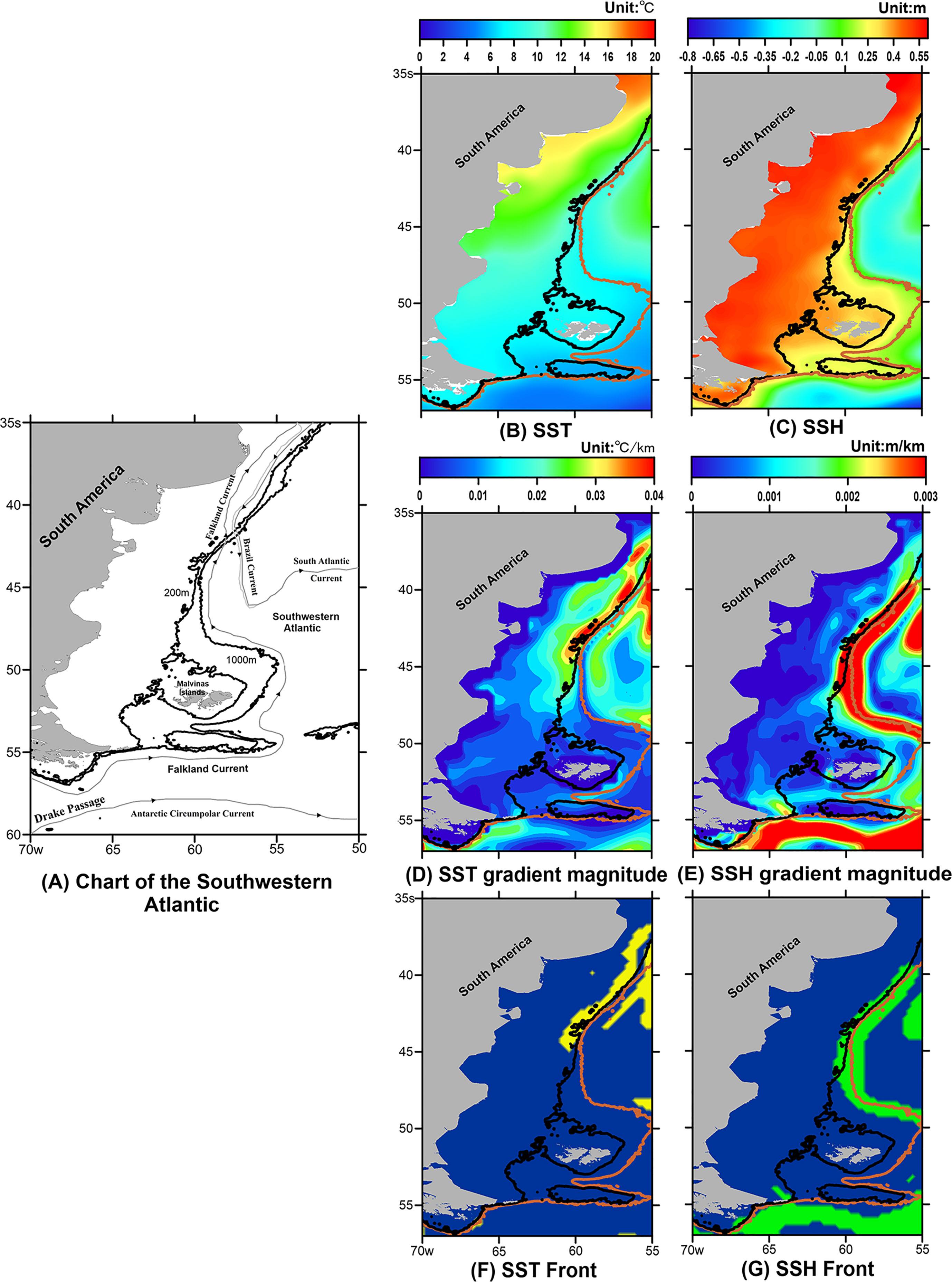
Figure 1 Introduction to the SAF background. (A) is the chart of the SA. (B, C) are 10-year (2010-2019) mean SST and SSH distributions over SA. (D, E) are mean SST and SSH gradient magnitude maps obtained from SST and SSH for 2010-2019. (F, G) are SST fronts (yellow zone) and SSH fronts (green zone) obtained from the corresponding gradient magnitude map by the threshold. The black and brown solid contours are 200m and 1000m isobaths, respectively.
In the frontal regions, the properties of water mass change rapidly, which are characterized with enhanced horizontal gradients of temperature, salinity, density, etc (Legeckis, 1979). Therefore, researchers often calculate the gradient magnitude map by gradient operation on satellite remote sensing observations (Text S1), and reserve the area with large gradient by a specific threshold to identify the ocean front (Moore et al., 1999; Dong et al., 2006; Wang et al., 2020). Among them, sea surface temperature (SST) data are widely used for ocean front detection (Freeman et al., 2016). Figures 1B, D, F are display the SST distribution over the SA, the SST gradient magnitude map, and the SST front (Southwestern Atlantic thermal front) obtained from the magnitude map by gradient threshold, respectively. Figure 1B shows that the temperature difference between the two sides of the 200m isobath is obvious. SST gradient magnitude map indicates the magnitude of the temperature gradient, which can reflect the intensity of the front. As can be seen from Figure 1D, the maximum SST gradient magnitude are mainly distributed along the west of the 200m isobaths, which coincides exactly with the spatial distribution of the SST front (yellow zone) in Figure 1F. Therefore, the Southwestern Atlantic thermal front (SST front) is mainly distributed along the South American shelf water on the western side of the 200m isobath. Apart from that, the SAF is a typical “current-induced front” (Wang et al., 2021) and thus has prominent dynamic characteristics. Since sea surface height (SSH) data can be used to represent the dynamic characteristics of ocean phenomena, they have been widely used in the study of dynamic fronts in recent years (Chambers, 2018). Figure 1C shows the SSH distribution over the SA. Different from the SST distribution, the SSH distribution is mainly divided by the 1000m isobath, which is exactly consistent with the pathway of the Falkland Current. The invasion of the South American shelf water by the Falkland Current along the 1000m isobath leads to the encounter of two water masses with different dynamic characteristics, resulting in a large difference in the SSH, thus generating the SSH front (Southwestern Atlantic dynamic front). According to Figures 1E, G, the Southwestern Atlantic dynamic front is mainly distributed along the 1000m isobath, which is different from the spatial distribution of the Southwestern Atlantic thermal front. It should be emphasized that for two distinct water masses, the fronts formed between them are unique. The reason for the difference in the spatial distribution of thermal and dynamic fronts comes from the different expression of front characteristics (Takahashi and Kawamura, 2005; Liu and Hou, 2012). Thermal front is the expression of the thermal characteristics of SAF, and the dynamic front is the performance of SAF’s dynamic characteristics. Both of them are part of SAF. Therefore, to achieve high-precision SAF detection that fuses dynamic and thermal characteristics cannot only rely on SST or SSH but requires the synergy of SST and SSH. Meanwhile, it is challenging to establish a feature association between massive SST and SSH data and accurately identify the SAF from complex feature fusion data (Liu et al., 2021). Traditional gradient-based frontal detection method (Text S1) cannot solve the above problems (Kittler, 1983).
In recent years, deep learning methods, especially convolutional neural networks (CNNs) have shown excellent performance in mining complex rules hidden in multi-source long term series data, and are increasingly applied to the study of various ocean phenomena such as mesoscale eddies, internal waves, and sea ice (Gao et al., 2022; Zhang and Li, 2022; Li et al., 2022a). Since ocean fronts separate water mass classes and neural networks are robust in assigning classes in complex data, edge detection driven by the underlying neural network may be a good way to find fronts (Li et al., 2022b). Compared with traditional frontal detection methods, deep learning methods have advantages in automatic feature extraction and modeling the relationship between multi-source remote sensing data and ocean fronts. This study develops a deep learning model, SAFNet, to perform feature fusion of SST and SSH data spanning 10 years (2010-2019), and extract the SAF from the fusion data. Comparative experiments show that SAFNet can achieve accurate detection of SAF. Finally, by comparing the seasonal frontal probability (FP) derived from SST, SSH and SST-SSH fusion data respectively, the necessity of the fusion data for SAF detection is proved, and a new understanding of the spatiotemporal distribution and seasonal variation of SAF is obtained. Apart from that, the code of the SAFNet will be updated to GitHub: https://github.com/yangxiaomao225/SAFNet.
The rest of the paper is organized as follows. Section 2 introduces the multi-source remote sensing data used to establish the dataset for training and testing the proposed model and the structure of the SAFNet. Some comparative experiments and spatiotemporal distribution of the FP are shown and discussed in Section 3. In the last section, some conclusions are drawn.
2 Data and method
2.1 Data for training and testing the deep learning model
The altimeter data used in this study are generated by Copernicus Marine and Environmet Monitoring Service (CMEMS) using data from the TOPEX/Poseidon, Jason-1, Jason-2, and Envisat missions. The daily gridded SSH data with a spatial resolution of 0.25°×0.25°from January 2010 to December 2019, spanning 10 years. Since SSH products contain two kinds of data, sea level anomalies (SLAs) and absolute dynamic topography (ADT), this study uses ADT, the sum of the time-mean dynamic topography and time-varying SLAs. The daily SST data with a 0.25° spatial resolution refers to the NOAA Optimum Interpolation (OI) SST product (Reynolds et al., 2007), which is constructed from infrared satellite observations of the Advanced Very High-Resolution Radiometer (AVHRR) and has the same period as the SSH data.
In this study, with the help of the above SSH and SST data, a SAF dataset is established for training and testing the proposed SAFNet. Since the Southwestern Atlantic thermal front (SST front) and dynamic front (SSH front) are part of the SAF and represent different oceanographic characteristics of the SAF, this study first uses the traditional gradient-based front identification method (Text S1) to calculate SST and SSH front through SST and SSH, respectively. Then, the union of the two kinds of fronts is used to represent the SAF in the ideal state, which incorporated the thermal and dynamic characteristics. We describe the creation of the dataset with two samples from the SAF dataset (Text S2; Figure S1).
Thus, SAFs obtained from SST and SSH data in the SA (35°S-57°S, 55°W-70°W, 128×128 pixels) during the period 2010-2018 are used as the training dataset and SAFs obtained from 2019 data are used as the validation dataset in this study. There are 3,287 training samples and 365 validation samples, and pixels in each sample are labeled as “1” or “0” for front or non-front, respectively.
2.2 SAFNet
2.2.1 Overall Structure of the SAFNet
To achieve accurate detection of the SAF by fusing multiple oceanographic features, the proposed deep learning model needs to simultaneously obtain dynamic and thermal characteristics from SSH and SST data, and can accurately detect SAF from these features. Through the traditional gradient-based front detection method (Text S1), we know that the front are the pixels with large gradients. Therefore, the proposed model needs to have two capabilities: 1) The pixels with large gradients in SST and SSH data are extracted and fused as key features. 2) Accurately extract the pixels with large gradients from the fusion features, so as to achieve high-precision detection of SAF. Thus, the SAFNet model consists of two sub-networks: a data fusion network (DFN) to establish the SSH-SST feature fusion relationship and a feature extraction network (FEN) to accurately identify pixels with large gradients from the fusion data for SAF detection. Considering the complex nonlinear relationship between SST and SSH in the SAF, the DFN is developed based on CNNs containing dense connections, and the FEN is developed based on U-Net (Ronneberger et al., 2015), a classical semantic segmentation network in deep learning, as shown in Figure 2. In order to show the detection performance of SAFNet, this study compared SAFNet with two deep learning models on the validation set for SAF detection accuracy. The first one is LinkNet (Chaurasia and Culurciello, 2017), a classical semantic segmentation model, and the other one is D-LinkNet (Zhou et al., 2018), which has achieved excellent results in the field of road recognition. Since they do not contain a data fusion module, to make a fair comparison, this study adds DFN to LinkNet and D-LinkNet so that the two models can fuse the features of SST and SSH like SAFNet.
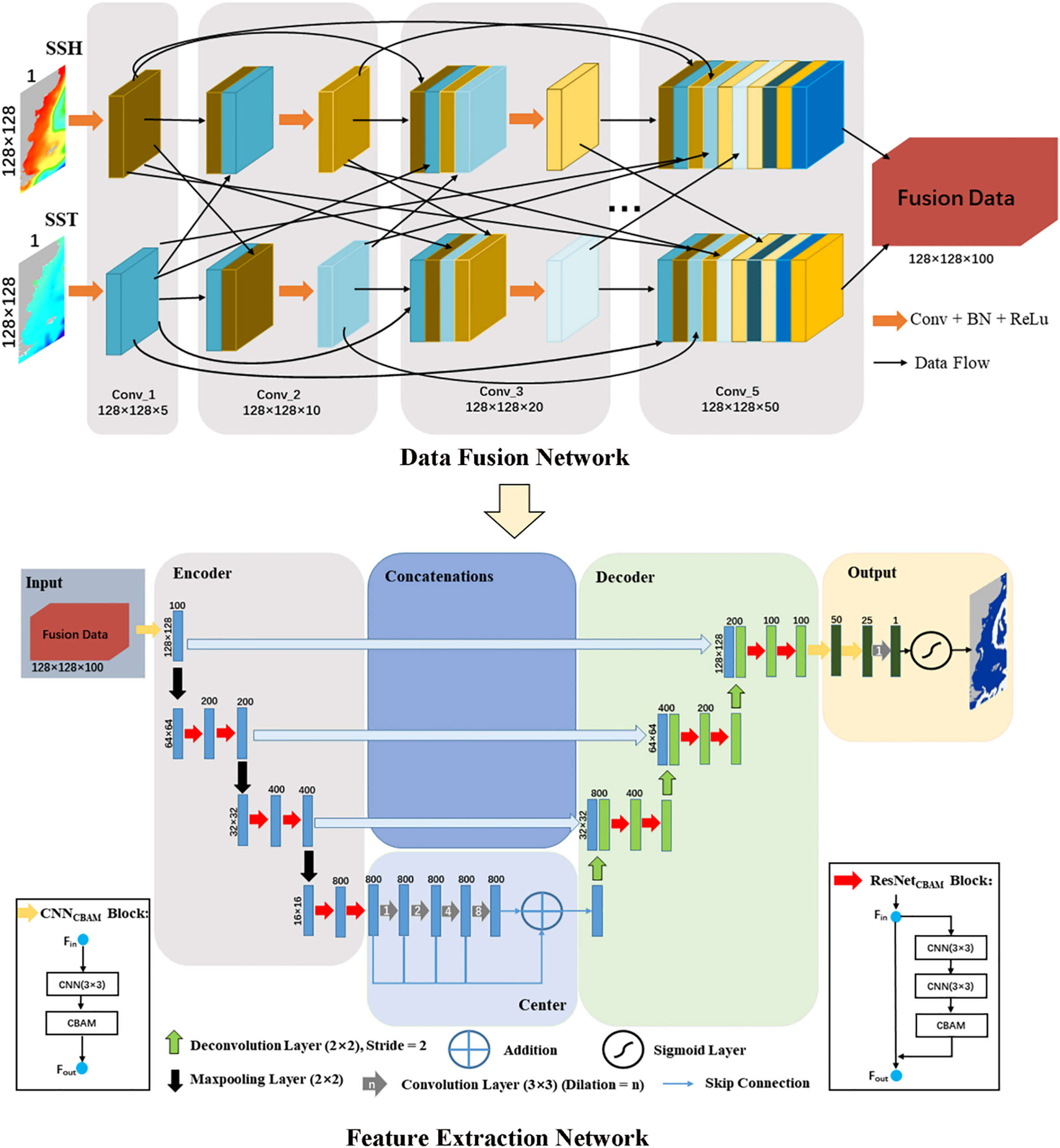
Figure 2 The overall structure of the SAFNet which consist of a data fusion network (DFN) and a feature extraction network (FEN).
2.2.2 DFN
Considering that different satellite sensors observe SSH and SST data, the fusion of two multi-source heterogeneous data belongs to multi-modal data fusion. Multi-modal data fusion based on deep learning is widely applied in medical image segmentation. There are three data fusion strategies: input-level fusion, layer-level fusion, and decision-level fusion (Zhou et al., 2019). Unlike the other two data fusion strategies, layer-level fusion can effectively integrate and fully use multi-modal data. In the layer-level fusion strategy, DenseNet (Huang et al., 2017) is the most commonly used network, so an improved DenseNet structure (Dolz et al., 2019) is used as the DFN in this study. The SSH and SST data with 128×128 pixels are imported into two different data streams, respectively, and the features of SSH and SST are extracted through the convolutional layers in the data stream. These features are densely connected between layer pairs in the same data stream and between layer pairs across data streams, and finally a fused data set combining SST and SSH features is obtained, as shown in Figure 2. The mathematical expression of DFN is as follows:
where refers to SSH or SST stream, denote the outputs of the th layer in SSH and SST streams and represents the mapping function of the two data streams at th layer composed of a convolution layer followed by a batch normalization and a Rectified Linear Unit (ReLU) activation function. Therefore, DFN can alleviate the vanishing gradient problem, introduce implicit deep supervision, and reduce the risk of overfitting tasks with smaller training sets.
2.2.3 FEN
In this study, the FEN is used to accurately detect the SAF based on the output of the DFN. To improve the detection accuracy, the convolutional block attention module (CBAM) (Woo et al., 2018) and dilated convolution layers (DCLs) are integrated into the FEN. FEN uses an encoder-decoder structure. The architecture of FEN includes six parts: input, encoder, center, decoder, concatenations and output. The goal of the encoder is to gradually extract pixels with large gradients from the fusion data through various convolutional layers, to capture the SAF features at different representation levels. The encoder contains one CNNCBAM block, six ResNetCBAM blocks, and three Max pooling layers. A CNNCBAM block is one CNN layer stacking with the CBAM, and a ResNetCBAM block is a ResNet unit integrated with the CBAM. The legend on the right in Figure 2 shows that a ResNet unit contains two CNN layers, stacking the CBAM after the second CNN layer. Adding the attention mechanism to the FEN can effectively capture the thermal and dynamic dependencies of the SAF at different scales. CBAM is divided into two modules: channel attention module and spatial attention module. These two modules can generate the feature map’s weight matrix in two dimensions. Then the weight matrices are multiplied by the input feature map for adaptive feature refinement so that the network is more targeted to extract features. The center part consists of several DCLs with skip connections. Considering the SAF’s narrowness, connectivity, and complexity, it is important to increase the receptive field of feature points in the center part and keep detailed information. DCLs are undoubtedly the best option. The decoder includes four stages, and between each stage, the scale of the feature map is restored by upsampling until the output feature map is the same size as the input data. Six ResNetCBAM blocks are integrated into the decoder to recover the SAF’s details accurately. The concatenation fuses the encoder and decoder at the same level, effectively preventing feature loss. The output consists of two CNNCBAM blocks, a 3×3 convolutional layer, and a sigmoid layer, finally outputs a value between [0,1]. If it is greater than 0.5, the pixel is the SAF; Otherwise, it is a non-front.
2.2.4 Loss function
Detection of the SAF is a typical binary classification problem, which only needs to determine which pixels are fronts and which are not. Therefore, the binary cross-entropy loss function (BCELoss) is an effective training method. However, classifying the pixels as front or non-front is a highly imbalanced problem. The weight of BCELoss cannot be set correctly when the specific difference between positive and negative samples is unknown, so the detection effect cannot be guaranteed. The dice coefficient loss function can improve this problem (Zhou et al., 2018). The dice coefficient is a measure function used to evaluate the similarity of two samples, with a larger value indicating more similarity and a smaller dice coefficient loss. Thus, this study defined the loss function as follows:
where the is the number of samples, is the detection result map of the SAFNet, is the SAF that has been labeled in the dataset. is the width of the feature map, is the height of the feature map, is a pixel in , and is a pixel in .
3 Results and discussion
3.1 Performance of SAFNet
The SAFNet is trained using the NVIDIA RTX A6000 48G GPU and PyTorch deep learning packages. The ADAM optimizer with the learning rate set to 0.01 and the learning rate decay set to 0.1 to optimize the model. The batch size and the number of epochs are set to 32 and 50.
Four metrics are adopted to evaluate the performance of SAFNet and the compared methods (LinkNet, D-LinkNet), i.e., Intersection over Union (IoU), Accuracy, Precision and Recall (Text S3). The objective evaluation results of the three models on the validation set are presented in Table S1. To visually show the differences of each model in SAF detection, the ground truth of four days are arbitrarily selected from the validation set and compared with the detection results of the three models. As shown in Figure 3, SAFNet achieves 99.45% detection accuracy for SAF, which is significantly better than the other two models. Since CBAM and DCLs are integrated in SAFNet, this study proves that CBAM and DCLs can effectively improve the detection accuracy of the proposed model for SAF through ablation experiments (Text S4; Table S2; Figure S2), which further proves that the SAFNet can be used as an effective tool to detect the SAF accurately.
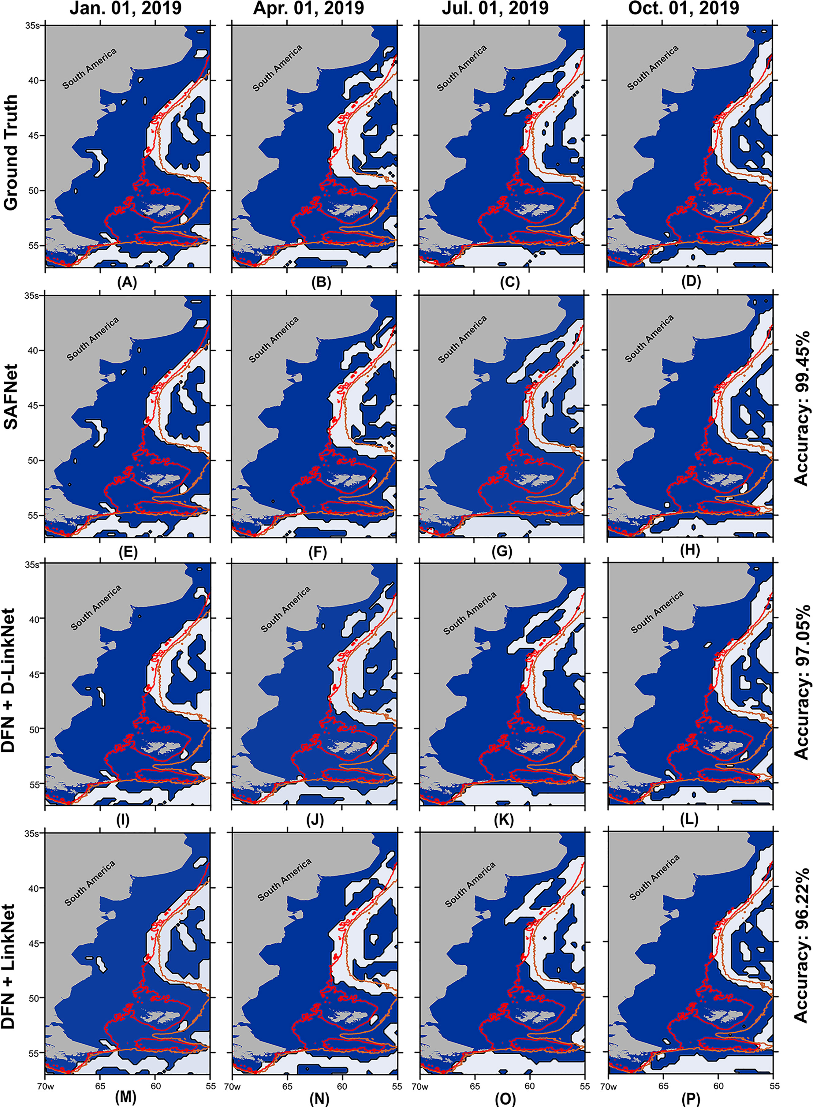
Figure 3 The results of the SAF detection. (A–D) are SAF ground truth of four days in validation set, the white zone represents the SAF, and the blue zone is the non-frontal zone. (E–P) are detection results of each model. The red and brown solid contours are 200m and 1000m isobaths, respectively.
3.2 Spatiotemporal distributions of the SAF
In this study, the comparison experiment and ablation experiment in Section 3.1 fully proves that SAFNet can achieve high-precision detection of SAF. This subsection will prove that the detection results of SAF based on SST-SSH fusion data can reflect the spatial distribution of SAF more comprehensively and accurately than that based on SST or SSH alone. In oceanography, researchers often approximate the spatiotemporal distribution of a front by obtaining its climatological distribution. At present, there are two main methods used to calculate the climatological distribution of fronts. The first one is to calculate the gradient magnitude of the mean SST or SSH data, and use the gradient magnitude map to represent the distribution of fronts. The other one is to use the daily front distribution to calculate the frontal probability (FP), and use the FP distribution to represent the distribution of fronts. The region with large gradient in the gradient magnitude map corresponds to the region with large probability of the FP distribution (Figure S3), so both the gradient magnitude and FP can accurately reflect the spatial distribution of the front (Wang et al., 2020). Since the detection result of SAFNet is the spatial distribution of daily SAF that fuses SST and SSH features, FP is used to represent the climatological mean distribution of the SAF in this study. The FP at each pixel is defined as follows:
where is the number of times that the pixel is identified as a front, is the total number of observation days.
Figure 4 displays the seasonal spatiotemporal distributions of the SAF FP obtained by SST, SSH and the SST-SSH fusion data from 2010 to 2019. By comparing the detection results of the three kinds of data, it is found that the frontal signal of the Southwestern Atlantic thermal front (derived from the SST data) is abundant in the South American shelf waters (within the 200m isobath), while the signal of the Southwestern Atlantic dynamic front (derived from the SSH data) is almost lost in the shelf waters. This is mainly because the current over the shelf does not organize into intensified velocity core or pattern, so that no outstanding SSH gradient exist. However, due to the invasion of the Falkland Current, the shelf water has obvious temperature differences, producing noticeable thermal characteristics (Text S5; Figure S4). Furthermore, the seasonal variation of the thermal front is obvious, which is stronger in summer and weaker in winter. The dynamic front is stable in four seasons and exists all the time. The reasons for this phenomenon come from two aspects: 1) In winter, the increasing surface cooling effects make SSTs uniform, leading to a decrease in the temperature difference between the Falkland Current and shelf water and the disappearance of the thermal front. 2) The Falkland Current intrudes into the shelf water all year around, resulting in the stable existence of SSH difference between water masses, so the distribution of dynamic fronts is relatively stable (Text S5; Figure S4). Hence, in the detection of the SAF, the thermal front has seasonal limitations and the dynamic front has spatial limitations, which indicates that neither the Southwestern Atlantic thermal front nor the dynamic front can fully accurately reflect the SAF. They only reflect the SAF’s thermal and dynamic characteristics, respectively (Text S5). The detection results of SAF by fusion data can fuse the information of the thermal front and the dynamic front and complement the advantages of the two fronts to realize the comprehensive and accurate detection of the SAF. Through the detection results of the fusion data, this study further understands the SAF distribution. North of 50°S, the SAF is mainly distributed along the continental slope break zone between the 200m and 1000m isobaths, and south of 50°S, the SAF is mainly distributed along 1000m isobath, as displayed in Figures 4L–O.
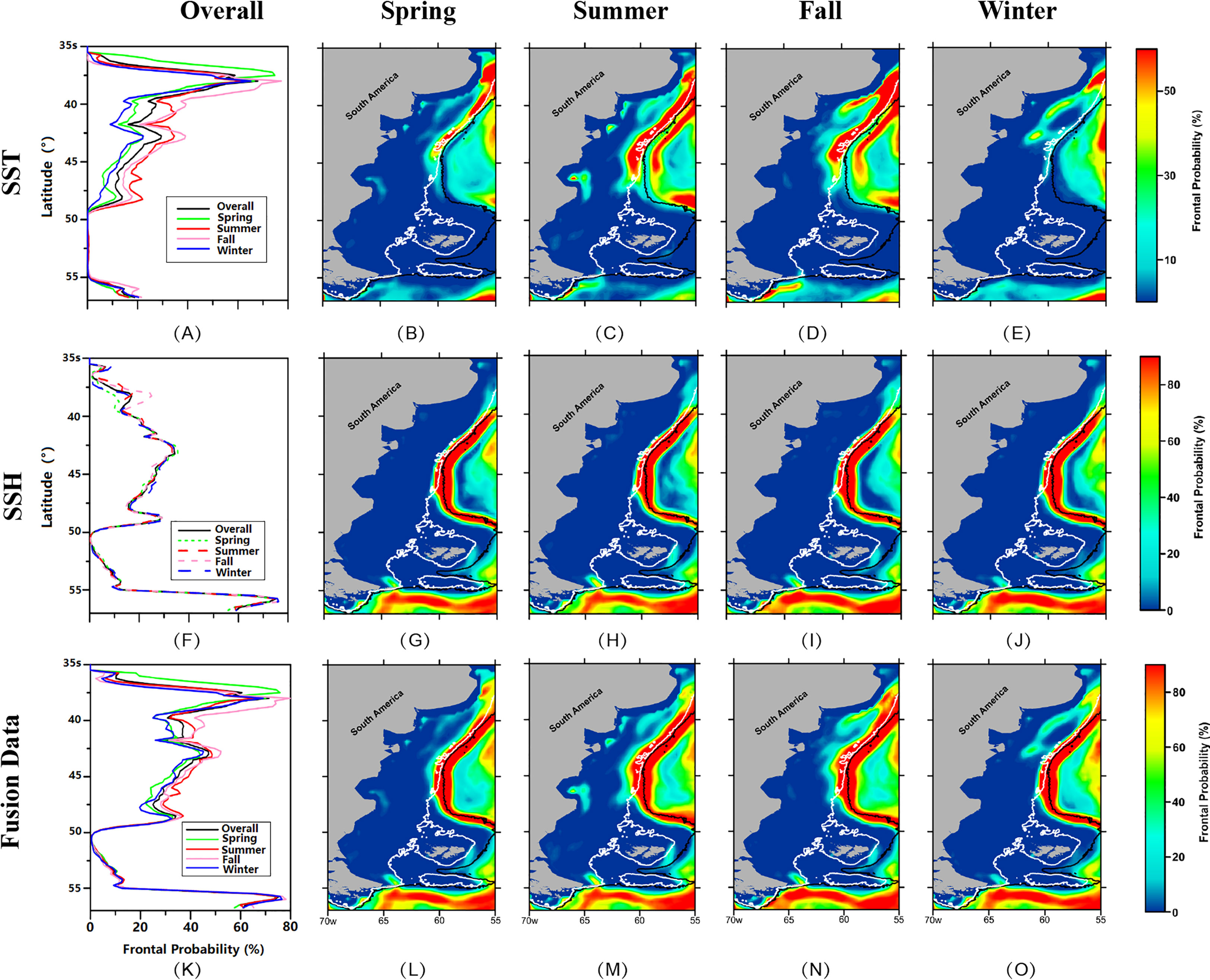
Figure 4 Spatiotemporal distributions of the SAF FP obtained by SST, SSH, and the fusion data from 2010 to 2019. The graphs and maps show meridional variation and seasonal spatial distribution of the SAF FP obatined by SST(A–E), SSH (F–J) and the fusion data (K–O).
Figures 4A, F, K display the meridional variation of the FP for detection results of three kinds of data. According to the above results, neither the thermal or dynamic front can represent SAF accurately and comprehensively. Therefore, through the meridional variation of the thermal and dynamic fronts, the changes of the thermal and dynamic characteristics of the SAF can be revealed. By comparing the three graphs, we know that the SAF has stable dynamic characteristics, and the main reason for the seasonal variation of the SAF is the change in its thermal characteristics. Between the 40°S and 50°S, SAF is stronger in summer and fall than in winter and spring, mainly because the temperature gradient between the shelf water and the Falkland Current is not obvious due to the spatially uniform surface cooling in winter. However, in the 35°S-40°S region, SAF is weakest in summer. This is mainly because this region is affected by the Brazil Current (a strong warm current) and has a high temperature, while the shelf water temperature is also high in summer, which makes the temperature gradient small and the front intensity weak in this region.
4 Conclusion
SAF is a typical current-induced front with prominent dynamic and thermal characteristics. Therefore, this study proposes the SAFNet that can fuse SST and SSH features over 2010-2019 and detect the SAF from the fusion data accurately, thus achieving an overall high-precision detection of SAF by fusing thermal and dynamic characteristics. The CBAM and DCLs are integrated into the SAFNet. The comparative experiments and ablation experiments show that SAFNet can achieve high precision detection of SAF, and the detection accuracy reaches 99.45%. By comparing the seasonal detection results of SAF FP obtained by SST, SSH, and the fusion of SST-SSH, this study finds that SAF is mainly distributed along the continental slope break zone of South America and the 1000m isobath. According to the meridional variation of FP, we know that the SAF has stable dynamic characteristics, and the reason for the seasonal difference of SAF is the change in its thermal characteristics. The SAF between 40°S and 50°S is weakest in winter due to the uniform surface cooling. In the 35°S-40°S region, the warm Brazil Current makes the water temperature generally higher and the temperature gradient is not obvious in summer, which leads to the weakest SAF.
Data availability statement
The original contributions presented in the study are included in the article/Supplementary Material. Further inquiries can be directed to the corresponding author.
Author contributions
CM: conceptualization. ZW: designed the experiments. GC, CM and YL: funding acquisition. ZW and YL: methodology. ZW: data processing. ZW: wrote the draft. GC and YL: review and validation. All authors contributed to the article and approved the submitted version.
Funding
This work was supported in part by the International Research Center of Big Data for Sustainable Development Goals under Grant CBAS2022GSP01, and in part by the National Natural Science Foundation of China under Grant 42276179 and 42030406, and in part by the Pilot National Laboratory For Marine Science and Technology (Qingdao) Laboratory open fund project under Grant 2019B02.
Conflict of interest
The authors declare that the research was conducted in the absence of any commercial or financial relationships that could be construed as a potential conflict of interest.
Publisher’s note
All claims expressed in this article are solely those of the authors and do not necessarily represent those of their affiliated organizations, or those of the publisher, the editors and the reviewers. Any product that may be evaluated in this article, or claim that may be made by its manufacturer, is not guaranteed or endorsed by the publisher.
Supplementary material
The Supplementary Material for this article can be found online at: https://www.frontiersin.org/articles/10.3389/fmars.2023.1140645/full#supplementary-material
References
Chambers D. P. (2018). Using kinetic energy measurements from altimetry to detect shifts in the positions of fronts in the southern ocean. Ocean Sci. 14, 105–116. doi: 10.5194/os-14-105-2018
Chapman C. C., Lea M. A., Meyer A., Sallee J. B., Hindell M. (2020). Defining southern ocean fronts and their influence on biological and physical processes in a changing climate. Nat. Climate Change 10, 209–219. doi: 10.1038/s41558-020-0705-4
Chaurasia A., Culurciello E. (2017). “LinkNet: Exploiting encoder representations for efficient semantic segmentation”, in IEEE Visual Communications and Image Processing (VCIP), St. Petersburg, FL, USA. 2017, 1–4. doi: 10.1109/VCIP.2017.8305148
Dolz J., Gopinath K., Yuan J., Lombaert H., Desrosiers C., Ben Ayed I. (2019). HyperDense-net: a hyper-densely connected CNN for multi-modal image segmentation. IEEE Trans. Med. Imaging 38, 1116–1126. doi: 10.1109/TMI.2018.2878669
Dong S. F., Sprintall J., Gille S. T. (2006). Location of the antarctic polar front from AMSR-e satellite sea surface temperature measurements. J. Phys. Oceanogr 36, 2075–2089. doi: 10.1175/JPO2973.1
Freeman N. M., Lovenduski N. S., Gent P. R. (2016). Temporal variability in the Antarctic polar front (2002–2014). J. Geophysical Res. 121, 7263–7276. doi: 10.1002/2016JC012145
Gao L., Li X., Kong F., Yu R., Guo Y., Ren Y. (2022). AlgaeNet: a deep-learning framework to detect floating green algae from optical and SAR imagery. IEEE J. Selected Topics Appl. Earth Observations Remote Sens. 15, 2782–2796. doi: 10.1109/JSTARS.2022.3162387
Huang G., Liu Z., Laurens V. D. M., Weinberger K. Q. (2017). Densely connected convolutional networks. In Proceedings of the IEEE conference on computer vision and pattern recognition (CVPR), Honolulu, HI, USA. pp. 4700–4708.
Kittler J. (1983). On the accuracy of the sobel edge detector. Image Vision Computing 1, 37–42. doi: 10.1016/0262-8856(83)90006-9
Legeckis R. (1979). A survey of worldwide sea surface temperature fronts detected by environmental satellites. J. Geophysical Research: Oceans 83, 4501–4522. doi: 10.1029/JC083iC09p04501
Li Y., Liang J., Da H., Chang L., Li H. (2022b). A deep learning method for ocean front extraction in remote sensing imagery. IEEE Geosci. Remote Sens. Lett. 19, 1–5. doi: 10.1109/LGRS.2021.3081179
Li X., Zhou Y., Wang F. (2022a). Advanced information mining from ocean remote sensing imagery with deep learning. J. Remote Sens. 2022. doi: 10.34133/2022/9849645
Liu Z., Hou Y. (2012). Kuroshio front in the East China Sea from satellite SST and remote sensing data. IEEE Geosci. Remote Sens. Lett. 9, 517–520. doi: 10.1109/LGRS.2011.2173289
Liu Y., Zheng Q., Li X. (2021). Characteristics of global ocean abnormal mesoscale eddies derived from the fusion of Sea surface height and temperature data by deep learning. Geophysical Res. Lett. 48. doi: 10.1029/2021GL094772
Lopes R. M., Marcolin C. R., Brandini F. P. (2016). Influence of oceanic fronts on mesozooplankton abundance and grazing during spring in the south-western Atlantic. Mar. Freshw. Res. 67, 626–635. doi: 10.1071/MF14357
Moore J. K., Abbott M. R., Richman J. G. (1999). Location and dynamics of the Antarctic polar front from satellite sea surface temperature data. J. Geophysical Research-Oceans 104, 3059–3073. doi: 10.1029/1998JC900032
Piola A. R., Franco B. C., Palma E. D., Saraceno M. (2013). Multiple jets in the malvinas current. J. Geophysical Research-Oceans 118, 2107–2117. doi: 10.1002/jgrc.20170
Reynolds R. W., Smith T. M., Liu C., Chelton D. B., Casey K. S., Schlax M. G. (2007). Daily high-resolution-blended analyses for sea surface temperature. J. Climate 20, 5473–5496. doi: 10.1175/2007JCLI1824.1
Ronneberger O., Fischer P., Brox T. (2015). U-Net: convolutional networks for biomedical image segmentation. Med. Image Computing Computer-Assisted Intervention Pt Iii 9351, 234–241. doi: 10.1007/978-3-319-24574-4_28
Takahashi W., Kawamura H. (2005). Detection method of the kuroshio front using the satellite-derived chlorophyll-a images. Remote Sens. Environ. 97, 83–91. doi: 10.1016/j.rse.2005.04.019
Wang Z., Chen G., Han Y., Ma C., Lv M. (2021). Southwestern Atlantic ocean fronts detected from satellite-derived SST and chlorophyll. Remote Sens. 13. doi: 10.3390/rs13214402
Wang Y., Yu Y., Zhang Y., Zhang H. R., Chai F. (2020). Distribution and variability of sea surface temperature fronts in the south China sea. Estuar. Coast. Shelf Sci. 240. doi: 10.1007/978-3-662-61834-9
Woo S., Park J., Lee J. Y., Kweon I. S. (2018). CBAM: Convolutional block attention module. In Proceedings of the European conference on computer vision (ECCV), Munich, Germany, pp. 3–19.
Zhang X., Li X. (2022). Satellite data-driven and knowledge-informed machine learning model for estimating global internal solitary wave speed. Remote Sens. Environ. 283. doi: 10.1016/j.rse.2022.113328
Zhou T., Ruan S., Canu S. (2019). A review: deep learning for medical image segmentation using multi-modality fusion. Array 3-4. doi: 10.1016/j.array.2019.100004
Keywords: Southwestern Atlantic fronts, multi-source remote sensing data, deep learning, ocean dynamics, ocean thermodynamics
Citation: Wang Z, Chen G, Ma C and Liu Y (2023) Southwestern Atlantic ocean fronts detected from the fusion of multi-source remote sensing data by a deep learning model. Front. Mar. Sci. 10:1140645. doi: 10.3389/fmars.2023.1140645
Received: 09 January 2023; Accepted: 31 May 2023;
Published: 14 June 2023.
Edited by:
Hongsheng Bi, University of Maryland, College Park, United StatesReviewed by:
Felipe Minuzzi, Federal University of Santa Maria, BrazilJian Zhao, University of Maryland, College Park, United States
Copyright © 2023 Wang, Chen, Ma and Liu. This is an open-access article distributed under the terms of the Creative Commons Attribution License (CC BY). The use, distribution or reproduction in other forums is permitted, provided the original author(s) and the copyright owner(s) are credited and that the original publication in this journal is cited, in accordance with accepted academic practice. No use, distribution or reproduction is permitted which does not comply with these terms.
*Correspondence: Chunyong Ma, Y2h1bnlvbmdtYUBvdWMuZWR1LmNu