Spatiotemporal distributions of air-sea CO2 flux modulated by windseas in the Southern Indian Ocean

Sun, Huiying; Zheng, Kaiwen; Yu, Jing; Zheng, Hao

doi:10.3389/fmars.2023.1139591

ORIGINAL RESEARCH article

Front. Mar. Sci., 01 March 2023

Sec. Coastal Ocean Processes

Volume 10 - 2023 | https://doi.org/10.3389/fmars.2023.1139591

This article is part of the Research Topic Extreme Weather Events Induced Coastal Environment Changes under Multiple Anthropogenic Impacts View all 16 articles

Spatiotemporal distributions of air-sea CO₂ flux modulated by windseas in the Southern Indian Ocean

Huiying Sun^1†

Kaiwen Zheng^2†

Jing Yu^1,3*

Hao Zheng^4,5*

¹College of Oceanic and Atmospheric Sciences, Ocean University of China, Qingdao, China
²Frontier Science Center for Deep Ocean Multispheres and Earth System (FDOMES), Physical Oceanography Laboratory, Ocean University of China, Qingdao, China
³Institute of Marine Development of Ocean University of China, Qingdao, China
⁴Key Laboratory of Marine Environment and Ecology, Institute of Coastal Environmental Pollution Control, College of Environmental Science and Engineering, Ministry of Education, Frontiers Science Center for Deep Ocean Multispheres and Earth System, Ocean University of China, Qingdao, China
⁵Sanya Oceanographic Institution, Ocean University of China, Sanya, China

The Southern Indian Ocean is a major reservoir for rapid carbon exchange with the atmosphere, plays a key role in the world’s carbon cycle. To understand the importance of anthropogenic CO₂ uptake in the Southern Indian Ocean, a variety of methods have been used to quantify the magnitude of the CO₂ flux between air and sea. The basic approach is based on the bulk formula—the air-sea CO₂ flux is commonly calculated by the difference in the CO₂ partial pressure between the ocean and the atmosphere, the gas transfer velocity, the surface wind speed, and the CO₂ solubility in seawater. However, relying solely on wind speed to measure the gas transfer velocity at the sea surface increases the uncertainty of CO₂ flux estimation. Recent studies have shown that the generation and breaking of ocean waves also significantly affect the gas transfer process at the air-sea interface. In this study, we highlight the impact of windseas on the process of air-sea CO₂ exchange and address its important role in CO₂ uptake in the Southern Indian Ocean. We run the WAVEWATCH III model to simulate surface waves in this region over the period from January 1^st 2002 to December 31^st 2021. Then, we use the spectral partitioning method to isolate windseas and swells from total wave fields. Finally, we calculate the CO₂ flux based on the new semiempirical equation for gas transfer velocity considering only windseas. We found that after considering windseas’ impact, the seasonal mean zonal flux (mmol/m²·d) increased approximately 10%-20% compared with that calculated solely on wind speed in all seasons. Evolution of air-sea net carbon flux (PgC) increased around 5.87%-32.12% in the latest 5 years with the most significant seasonal improvement appeared in summer. Long-term trend analysis also indicated that the CO₂ absorption capacity of the whole Southern Indian Ocean gradually increased during the past 20 years. These findings extend the understanding of the roles of the Southern Indian Ocean in the global carbon cycle and are useful for making management policies associated with marine environmental protection and global climatic change mitigation.

1 Introduction

Human activities have been a major source of global warming over the past 50 years (IPCC, 2022a). Anthropogenic emissions of greenhouse gases have persisted since 1990. By 2019, carbon dioxide (CO₂) from fossil fuels and industry had the largest growth in absolute emissions (IPCC, 2022b). Although CO₂ accounts for approximately 20% of greenhouse gases, it is responsible for 80% of the radiative forcing that sustains the greenhouse effect and makes the atmospheric temperature continuously rise (Lacis et al., 2010; Schmidt et al., 2010). Since the beginning of the industrial era, global anthropogenic CO₂ emissions from human activities such as the burning of fossil fuel, cement production, and changing land use have increased over time, and the present atmospheric carbon concentration has been unprecedented in the last three million years (Willeit et al., 2019). The accumulation of discharged atmospheric CO₂ rose from 277 ppm in 1750 to 414.4 ppm in 2021, well beyond the normal range of natural variability (Levitus et al., 2000; Feely et al., 2001; Joos and Spahni, 2008; Lekshmi et al., 2021). Therefore, the accurate evaluation of anthropogenic emissions and the world’s carbon cycle has been of great scientific interest in recent years.

The ocean is an important active carbon reservoir, taking up more than 25%-30% of anthropogenic CO₂ emitted to the atmosphere; so it plays a pivotal role in mitigating global climate change (Sabine et al., 2004; Friedlingstein et al., 2020). The Southern Indian Ocean, spanning from 0° to 66.5°S, is one of the largest oceanic sinks of anthropogenic CO₂, representing approximately 10% of the ocean surface area but removing 15% of CO₂ emitted by humans (Frölicher et al., 2015; Gruber et al., 2019). The Southern Indian Ocean is unique because of its geographical features, atmospheric forcing, and complex ocean dynamics. In contrast to the Pacific and the Atlantic, it is completely enclosed by the Indian subcontinent in the north and is dominated by westerlies near the equator rather than trade winds (Valsala et al., 2012). Annual wind speeds in this region are higher than those of other seas at the same latitudes, which increases the gas transfer velocity and thus accelerates the CO₂ exchange between the sea surface and atmosphere (Deacon, 1977; Wanninkhof, 2014; Watson et al., 2020).

To understand the importance of anthropogenic CO₂ uptake in the Southern Indian Ocean, a variety of methods have been used to quantify the magnitude of the CO₂ flux between the sea and air (Metzl et al., 1995; Louanchi et al., 1996). Typical approach based on the bulk formula—the air-sea CO₂ flux is commonly calculated by the difference in CO₂ partial pressure between the ocean and the air ( $p C O_{2}^{s e a}$ and $p C O_{2}^{a i r}$ , respectively), the gas transfer velocity, contemporaneous sea surface wind speed, and the CO₂ solubility in seawater (Takahashi et al., 2002; Sabine et al., 2004; DeVries, 2014; Frölicher et al., 2015; Roobaert et al., 2019). Using this approach, a series of crucial results have been reported in the last 20 years (e.g., Bates et al., 2006; Wanninkhof and Triñanes, 2017; Vieira et al. 2020). However, relying solely on wind speed to calculate the gas transfer velocity at the sea surface increases the uncertainty of CO₂ flux estimation (Woolf, 1993). Recent studies have shown that the generation and breaking of ocean waves also significantly affect the gas exchange process at the sea-air interface (Zappa et al., 2007; Gu et al., 2021). Observations in the Southern Indian Ocean sector of the Antarctic Circumpolar Current (ACC) show that large quantities of bubbles produced by wave breaking enhance the intensity of under-surface turbulence by up to three orders of magnitude and hence expand the gas contact area (Li et al., 2021). This will substantially increase gas transfer velocity and thus enhance CO₂ absorption by the ocean. To address the important role of surface wave breaking on CO₂ exchange, a new semiempirical equation for gas transfer velocity has recently been proposed that can account for different significant wave height (SWH hereafter) and divide gas transfer velocity into turbulence and bubbles contributions. Calculations after this upgrade significantly reduce the uncertainty of gas transfer velocity at moderate-high wind speeds (Deike and Melville, 2018). And the contribution of bubbles and the dependence of the ocean state vary greatly on regional and seasonal scales, generally supporting the ocean to absorb approximately 40% of the CO₂ (Reichl and Deike, 2020). Gu et al. (2021) investigated a new expression of gas transfer velocity that coupled with wind-wave and showed that about 50% of the global CO₂ fluxes at high wind speeds are attributable to bubble-mediated contributions. However in these studies, ‘wind-wave’ represents total waves and using these to modulate gas transfer velocity may exaggerate their impacts.

Surface waves consist of swells and windseas, which are two categories with completely different characteristic features (Wang and Huang, 2004). Swells usually have regular shapes, more orderly arrangements with longer crest lines and smooth surfaces. They are stable as due to the action of air resistance and the internal friction of sea water, the wave energy is distributed in a larger area, and the energy and wave height of a swell in the water column decrease continuously during propagation (Zhang et al., 2011; Ethamony et al., 2013). As the period increases, the wavelength and wave speed grow correspondingly, which makes the steepness of the wave surface decrease. Hence swells will not produce large numbers of bubbles in the sea-air interface. In contrast to swells, windseas are locally generated, have short wavelengths, are more chaotic, and travel more slowly than surface wind. Windseas gain energy from wind to grow and easily lose instability and break, which significantly affects the gas exchange process in the sea-air interface (Qian et al., 2020). Now that total waves include two categories, using total waves to quantify the gas transfer velocity might overestimate the impact of waves on the overall CO₂ flux.

Therefore, in this study, we highlight the influence of windseas on air-sea CO₂ exchange process and address the important role of surface waves in CO₂ absorption in the Southern Indian Ocean. We run the WAVEWATCH III model to simulate surface waves in the Southern Indian Ocean over the period from January 1^st 2002 to December 31^st 2021. Then, we use the spectral partitioning method to isolate windseas and swells from total wave fields. Finally, we calculate CO₂ flux based on the new semiempirical equation for gas transfer velocity considering only windseas. The article is structured as follows. Section 2 discusses the model configuration of the simulations and the data source we used to validate the model output. Spectral partitioning method to separate windseas and swells are discussed. We also present the standard bulk formula of air-sea CO₂ exchange flux and bulk formula modulated by windseas in this section. Section 3 first shows the simulated results of the spatial and seasonal distributions of the SWH of windseas and swells in the Southern Indian Ocean. Then, the validation results of the model output and observation data are discussed. Finally, the temporal and spatial distributions of air-sea CO₂ exchange flux modulated by windseas, differences between the calculations with/without waves’ impact, and decadal trends of net carbon flux are presented. The overall implication and limitations of the study are evaluated in Section 4.

2 Data and methods

2.1 Configuration of wave simulations

We use the recent WAVEWATCH III (WW3, hereafter) official version 4.18 to simulate surface waves in the Southern Indian Ocean, spanning from 0° to 66.5°S. The specific settings are as follows: The wind speed—the 10 m wind above the surface—obtained from the European Centre for Medium-Range Weather Forecasts (ECMWF) ERA-5 datasets over the period from January 1^st 2002 to December 31^st 2021. The wind fields are regularly gridded and from 0° to 66.5°S, 30°E to 135°E with a 1/4° resolution. The time resolution is set to 6 hours. The water depth is automatically generated by the Gridgen 3.0 topography packet, which combines the National Geophysical Data Center - ETOPO 1 data. The topography resolution is 1/20°. Our model integrates the spectrum to a cut-off frequency f_HF and uses a parametric tail to frequency above f_HF. Twenty-four discrete wavenumbers (0.0412∼0.4060Hz, 2.4∼24.7s) and 36 directions are used to simulate isotropic waves. Parameterizations for current waves, wave-wave interactions, wave breaking-related white capping, wave refraction and shoaling are added to further improve the accuracy of the simulated waves (Hanson et al., 2006). Field model results, including 10-m wind speed, SWH of total waves, and wave energy density spectra, are output at each grid point with a time interval of 6 hours. We also output 4 points’ wave information according to the position shown in Figure 1, which will be used for model validation against altimeters in the following section 2.2. Although ERA-5 datasets also provide wave reanalysis data that contain partition results of swells and windseas, significant numerical and physical differences can still be found between the WW3 and WAM models (Liu et al., 2002).

FIGURE 1

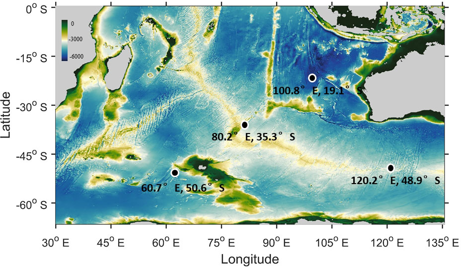
Figure 1 A map of the study region showing water depth in the Southern Indian Ocean, with the altimeter locations used for model verification. Four positions (60.7°E 50.6°S; 80.3°E 35.3°S; 100.8°E 19.1°S; 120.2°E 48.9°S) are randomly picked over a period from January 1^st 2021 to December 31^st 2021.

2.2 Modelling validation

In this study, we use altimeter data to evaluate our model performance. Data are obtained from the Australian Integrated Marine Observing System (IMOS), CRYOSAT-2 altimeter database. This data source provides global wave observations from altimeter products that have been put to use since 1985. All the wave heights have been verified against global float/buoy data at all crossover points with independent missions. Calibration details can be found in Ribal and Young (2019). In this study, we randomly selected four positions (shown in Figure 1) over a period from January 1^st 2002 to December 31^st 2021, for model validation. The SWH of total waves simulated by the WW3 model were compared to the altimeter data through temporal correlation analyses. We also calculated the bias and correlation coefficient between the model output and altimeter data to quantify the comparison results. All results are shown in Figure 2. The SWH produced by the model shows a clear temporal correlation with real-time data altimeter observations. The correlation indexes are over 0.75-0.84, and the biases are less than 0.17-0.32 in all four positions, indicating that our model basically reflects the main wave information in the Southern Indian Ocean.

FIGURE 2

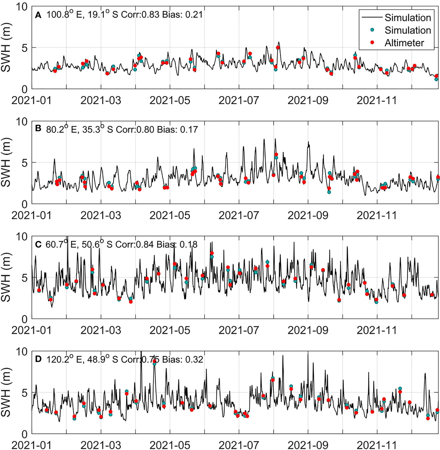
Figure 2 Time series of SWH comparisons between model outputs and altimeter records. Scatter points are results of model (green) and altimeter (red) correspond to a same moment. (A–D) are four panels of the four randomly selected locations.

2.3 The spectra energy partition method

The version of WW3 used in this study contains a partition module that can separate swells and windseas from total waves. The partition module was at first used as the topography processing watershed algorithm by Hanson and Jensen (2004) to isolate a 2D wave spectra. Then, modified FORTRAN routines (Hanson et al., 2006) were added into the WW3 model to identified different waves. The basic principle is inverting 2D wave spectra and making spectral peaks become catchments. Then partition boundaries or watershed lines can be identified using the watershed algorithm. Swells and windseas are determined using wave age criterion on the basis of different components of wind direction and absolute speed. This method has proven to be highly accurate and were added into the WW3 model to identified different waves (Zheng et al., 2016; Tao et al., 2017; Anoop et al., 2020).

2.4 Calculation of air-sea gas exchange flux with no waves

We calculated the air-sea gas exchange flux of CO₂ (F,mol/m²·d) with no waves using a standard bulk formula by Wanninkhof (2014):

\begin{array}{l} F = k_{0} L Δ p C O_{2} & (1) \end{array}

where positive values of Fdenote the transfer of CO₂ from the ocean towards the atmosphere, negative values correspond to that from the atmosphere into the ocean, and L (mol(kg·atm)^-1) is the solubility of CO₂ in water (Weiss, 1974):

\begin{array}{l} l n L = A l + A 2100 S S T + A 3 l n 100 S S T + S S S B 1 + B 2 S S T 100 + B 3 S S T 1002 & (2) \end{array}

Here, we used A₁ = -60.2409, A₂ = -93.4517, A₃ = 23.3585, B₁ = 0.023517, B₂ = -0.023656, and B₃ = 0.0047036. In addition, SST is the sea surface temperature in degrees Celsius and SSS is the sea surface salinity. k₀ is the appropriate gas transfer velocity calculated as $k_{0} = 0.251 U_{10}^{2} {(S c / 660)}^{- 0.5}$ , where U₁₀ is the wind speed measured 10 m above the sea surface. The constant value of 0.251 is based on an extensive collection of gas transfer velocity estimates from Wanninkhof (2014). The variable Sc is the Schmidt number:

\begin{array}{l} S c = a + b (S S T) + c {(S S T)}^{2} + d {(S S T)}^{3} & (3) \end{array}

where a = 2073.1,b =125.62, c = 3.6276, and d = 0.043219 are all constant values applied from parameterization by Wanninkhof (2014). $Δ p C O_{2} (p C O_{2}^{s e a} - p C O_{2}^{a i r})$ is the CO₂ partial pressure difference between the surface seawater and the air.

We calculated F for each 1/4° × 1/4° latitude-longitude grid point in the open water of the Southern Indian Ocean over the period 2002 to 2021. For variables, the following data products were used. Monthly mean SSTs were employed from the Advanced Microwave Scanning Radiometer (AMSR) datasets with two satellites provided by the Romete Sensing System, namely, AMSR-2 and AMSR-E. U₁₀ is an ERA-5 dataset of ECMWF from 1979 to the present. Monthly mean SSS is available at the Physical Sciences Laboratory (PSL) of the National Oceanic and Atmospheric Administration (NOAA). SSS is a product of the NCEP Global Ocean Data Assimilation System, which is forced by the momentum flux, heat flux, and fresh water flux from the NCEP atmospheric reanalysis (GODAS, Behringer et al., 1998). It reproduces observations well and is now the most commonly used dataset for F analysis (e.g., Watson et al., 2020; Monteiro et al., 2020; Zheng et al., 2021). For the ΔpCO₂, we employed the observation-based global monthly gridded atmospheric and sea surface CO₂ partial pressure and CO₂ fluxes product by Landschützer et al. (2020) from 1982 onwards. These observation-based data were obtained using a two-step artificial neural network method combining biogeochemical provinces and CO₂ driver variables and observations from the fourth release of the Surface Ocean CO₂ Atlas (SOCAT, Bakker et al., 2016).

2.5 Calculation of air-sea gas exchange flux with waves

To stress the important role of ocean surface waves in air-sea CO₂ exchange, we used a wind-wave-dependent expression by Deike and Melville (2018) to estimate the CO₂ exchange rate, k_w. k_w consists of two terms, bubble-mediated k_wb and nonbubble k_wnb, given as:

\begin{array}{l} k_{w} = k_{w b} + k_{w n b} = \frac{A_{B}}{L \cdot R \cdot S S T} u_{*}^{5 / 3} {(g H_{s})}^{2 / 3} {(\frac{S c}{660})}^{- 1 / 2} + A_{N B} u_{*} {(\frac{S c}{600})}^{- 1 / 2} & (4) \end{array}

where A_B = 1 ± 0.2 × 10^-5s²m^-2 is a dimensional fitting coefficient, A_NB = 1.55 × 10^-4, R = 0.08205 L atm mol^-1k^-1is the ideal gas constant (Keeling, 1993), g is the gravitational acceleration, and H_s is the SWH from the WW3 model simulated waves. $u_{*} = {(\frac{τ}{ρ_{a i r}})}^{1 / 2}$ is the friction velocity in the air, where ρ_air is the mean air density and τ is a turbulent shear stress. Then, the calculated k_w is substituted into equation (1) to further calculate the F under the impact of waves. The data sources used in this study are listed in Table 1.

TABLE 1

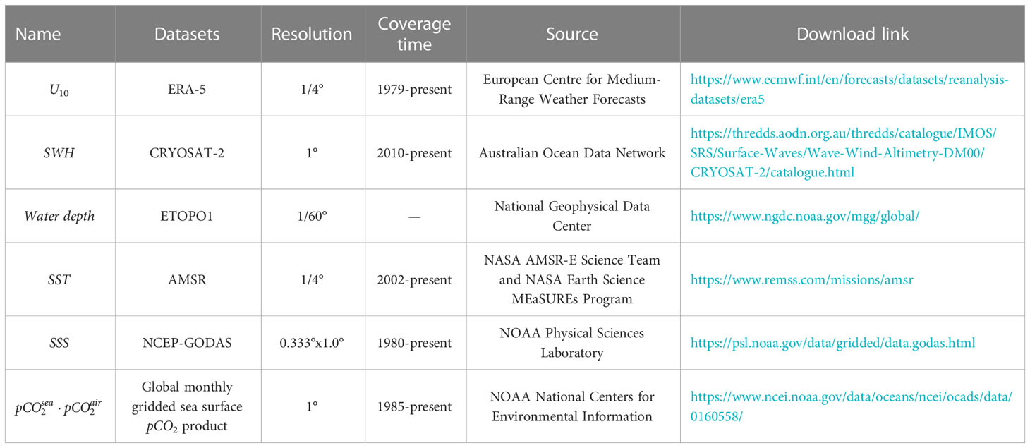
Table 1 Descriptions of data used in this study and their sources.

3 Results

3.1 Separation of swells and windseas from total waves in the Southern Indian Ocean

Seasonal distributions of SWH (including total waves, windseas, and swells) are showed in Figure 3. The highest seasonal mean SWH of total waves, windseas and swells are found in the extratropical areas, which are basically distributed along the southern westerlies. SWH also shows obviously seasonal variations in the whole Southern Indian Ocean. The strongest wave energy appears in summer, followed by winter. The wave heights depend greatly on the seasonal changes in wind speed; windseas are clearly aligned with the winds, as powerful westerly winds directly generate strong windseas (Semedo et al., 2011). The westerly region in the Southern Indian Ocean are the main source areas of swells (Vincent and Soille, 1991) also make swells energy particularly high than low-latitude region. Apart from these seasonal and spatial results that are consistent with previous surface wave studies (Zheng et al., 2016), our partition results provide an interesting view: windseas contribute only a small fraction of energy to the total waves in almost every region and season. In high- and middle-latitude areas (30°S-60°S), the windseas energy in winter accounts for the largest proportion, 37.26%, followed by summer, which is 25.09%. In low- and middle-latitude areas (0-30°S), summer and winter also have a higher windseas proportion but maintain less than 40% of total waves. As we discussed above, windseas have completely different physical properties with swells and should be the main factor influencing gas transfer velocities (Jiang and Chen, 2013). We suggest that modifying the air-sea CO₂ exchange flux by using total waves tends to overestimate the effect of waves. The specific proportion of windseas energy to total waves is shown in Table 2. In the following sections, we emphasize the effect of windseas on the air-sea CO₂ exchange flux in the southern Indian Ocean.

FIGURE 3

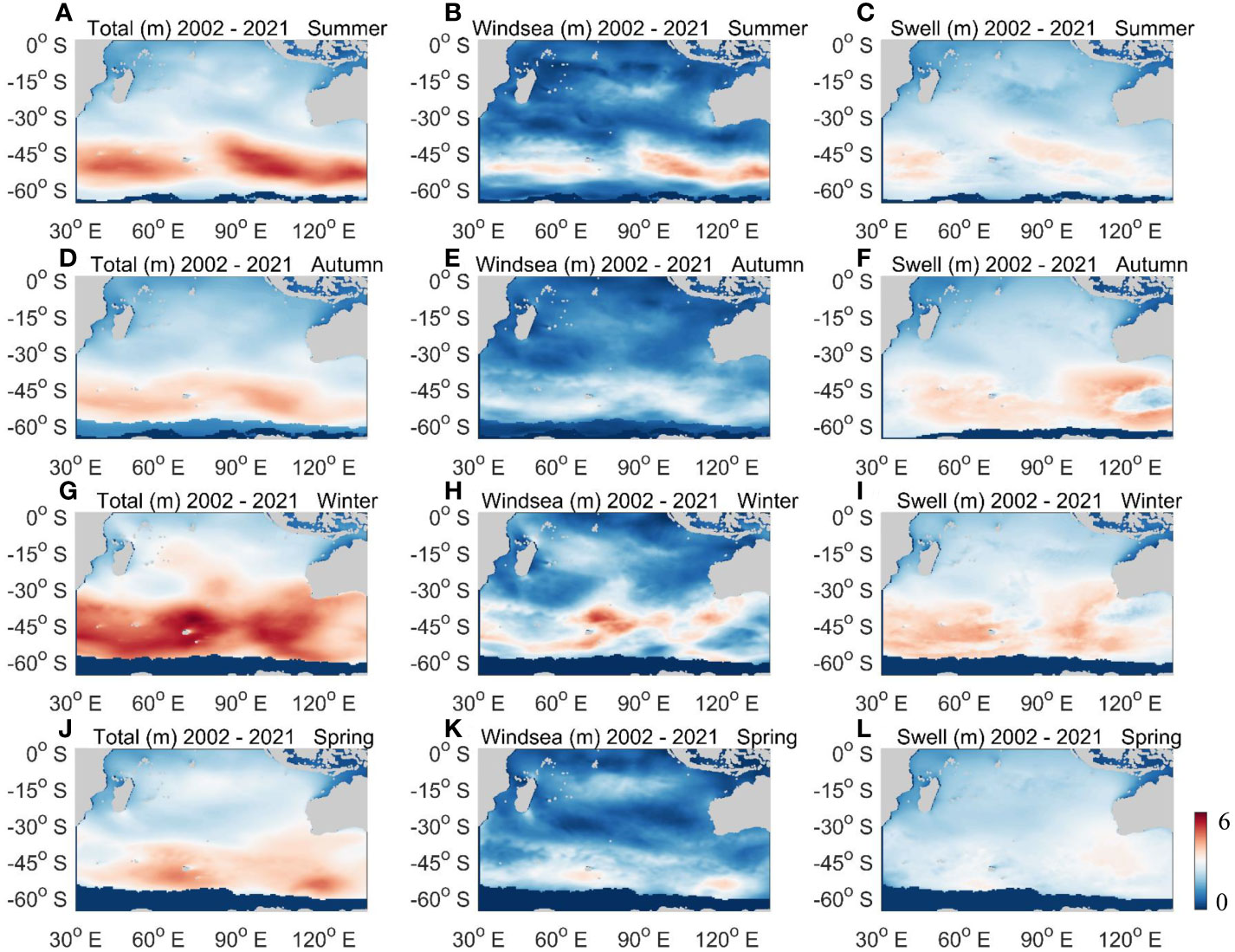
Figure 3 Seasonal averages for total SWH (A, D, G, J), wave height of windseas (B, E, H, K), and wave height of swells (C, F, I, L) in the Southern Indian Ocean.

TABLE 2

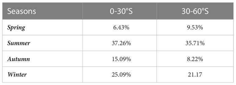
Table 2 The regional partition distribution of windseas energy to total waves in different seasons.

3.2 Spatial and temporal characteristics of air-sea CO₂ flux modulated by windseas

We first showed an important but independent driver—surface seawater partial pressure $(p C O_{2}^{s e a})$ —that affects air-sea CO₂ transfer in the Southern Indian Ocean. Because the atmospheric partial pressure of CO₂ $(p C O_{2}^{a i r})$ is nearly consistent in the open ocean, $p C O_{2}^{s e a}$ largely determines the direction and rate of CO₂ transfer through the air-sea interface (Takahashi et al., 2002). Study has shown that the majority of the seasonal and spatial variations in CO₂ flux stem from the $p C O_{2}^{s e a}$ (McGillis et al., 2001). Therefore, here, before carefully discussing the distribution and variation of the air-sea CO₂ flux, we first examined the spatial distribution of the seasonal mean $p C O_{2}^{s e a}$ in the Southern Indian Ocean (Figure 4). The spatial pattern of $p C O_{2}^{s e a}$ showed an uneven distribution, and seasonal variation was also apparent. In autumn and winter, there was a large area of low $p C O_{2}^{s e a}$ in the wide sea area between 20°S and 40°S. In addition, as the area of the subtropical high-pressure belt increased with the onset of spring, a decrease in the low $p C O_{2}^{s e a}$ area occurred from south to north. A high $p C O_{2}^{s e a}$ zone emerged near 80°E and reached its maximum value of 380 μatm. In summer, the low $p C O_{2}^{s e a}$ region tended to be stable at approximately 40°S, and $p C O_{2}^{s e a}$ followed by sea surface temperature variations. The $p C O_{2}^{s e a}$ in the Antarctic coastal waters was higher in autumn and winter, and lower in other seasons. Throughout the year, a high $p C O_{2}^{s e a}$ zone existed between 0°S and 12°S on the east coast of Africa, which was caused by the high-salinity and high-temperature water at the confluence of cold and warm currents in summer and the confluence of warm currents in winter (Deacon, 1981).

FIGURE 4

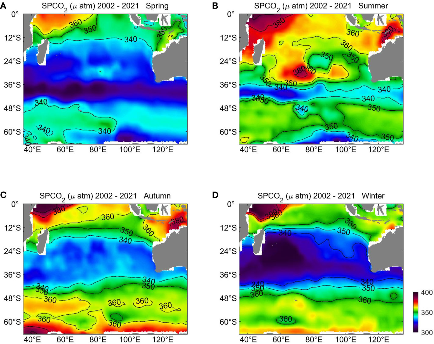
Figure 4 Seasonal distributions of surface seawater partial pressure of CO₂, $p C O_{2}^{s e a}$ (μatm), in the Southern Indian Ocean. (A) Spring, (B) Summer, (C) Autumn, (D) Winter.

Surface wave breaking has an effect on gas transfer velocity. A higher gas transfer velocity will be generated for more developed windseas states under the same wind and $p C O_{2}^{s e a}$ (Zhao et al., 2003). To see this difference clearly, we show the temporal evolution of the gas transfer velocity with waves and no waves in Figure 5. Values at each point are annually averaged in the full region. It is clear that after considering the impact of windseas, the gas transfer velocity is improved nearly for all times. An average 5%-15% enhancement is seen, which is lower than the enhancement caused by total waves shown in Gu et al. (2020). This is in line with expectations, as increasing evidence has indicated that mass transfer, such as CO₂, is factually influenced by the surface turbulent process associated with the wave field (Liang et al., 2013; Brumer et al., 2017; Lenain and Melville, 2017). Surface wind is just an external forcing; as an indirect factor, it does not determine gas exchange (e.g., Edson et al., 2011; Liang et al., 2020). However, if windseas break, they generate large amounts of whitecaps, which will directly affect gas transfer through two mechanisms. First, breaking waves can promote the transfer associated with the upper turbulent patches. The interface contaminated by surface active impurities can be renewed by breaking waves, resulting in an accelerated increase in gas exchange in high wind speed areas (Komori and Misumi, 2002). Then there is a bubble-mediated transfer, in which the gas is trapped in a bubble for a certain period of time during the transfer between the air and the sea (Hasse and Liss, 1980).

FIGURE 5

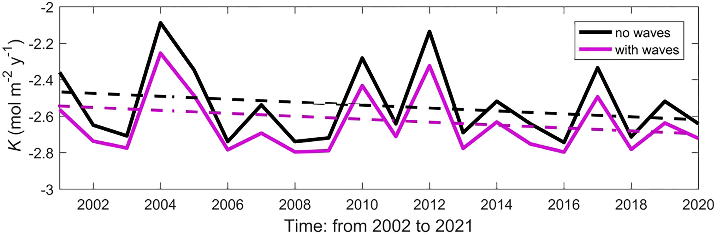
Figure 5 Temporal evolution of gas transfer velocity with waves (solid black) and no waves (solid purple).

Based on the new gas transfer velocity, we then provide the distributions of seasonal mean CO₂ flux modulated by windseas in the Southern Indian Ocean in Figure 6. The distribution of CO₂ flux in the Southern Indian Ocean exhibited distinct regional and seasonal differences. The tropical area (0°-12°S) tended to lose a substantial amount of CO₂ through outgassing, mainly due to the high SST and low wind speeds throughout the year. Among them, the CO₂ uptake in summer was weak over the regions because of the uniform distribution of air pressure and the relative scarcity of low pressure systems in the atmosphere. Compared with the tropical area, the seasonal variation of CO₂ flux in the subtropical region (12°S-36°S) was more obvious. During the spring and winter, the ability to absorb atmospheric CO₂ tended toward to be stronger than other seasons. In winter, controlled by the surface waves in the southeasterly trade winds, the CO₂ flux varied markedly. Strong trade winds in winter produced stronger wave fields leading to higher CO₂ flux, with an average maximum of -3.14 mmol/m²·d in the central region between 12°S and 24°S. In the ACC region (36°S-52°S), the Southern Indian Ocean was a very strong sink of atmospheric CO₂ throughout the year, with the maximum mean uptake reaching -8.12 mmol/m²·d. Strong westerly winds blowing across the sea give rise to abundant physical oceanographic processes, such as wind blocking, string, and high-pressure collapsing, may further strengthen the effect of windseas on the air- sea gas exchange (Toba and Koga, 1986; Toba, 1988). The majority of the net uptake occurred in winter, consistent with the findings of previous studies (Sarma et al., 2013; Zhang et al., 2017). Finally, similar to the tropical region, the entire subpolar region (52°S-62°S) tended to be a source of CO₂ to the atmosphere, because the horizontal temperature distribution was more uniform, the horizontal pressure gradient was very small, the air flow mainly converged and rose, the annual average wind speed is low which was unfavorable to the gas exchange process at the air-sea interface. Overall, annual mean value over the subpolar region is around -0.24 mmol/m²·d. To clearly show the impact of windseas to the CO₂ flux, we show differences for the seasonal and spatial distributions between with and without windseas impact in Figure 7. Consistent with the regional distributions of partition results of windseas from total waves, the most significant differences appears in the southern westerlies areas. And for the seasonal aspect, the strongest CO₂ uptake increasement appears in summer and winter. The maximum increasement gets up to 20% which suggests that the windseas have considerable impact in the region. In contrast, low-latitude region and spring and autumn all have a relatively weak increasement response to the low energy of windseas there.

FIGURE 6

Figure 6 Seasonal distributions of air-sea CO₂ flux, F (mmol/m²·d), in the Southern Indian Ocean. (A) Spring, (B) Summer, (C) Autumn, (D) Winter.

FIGURE 7

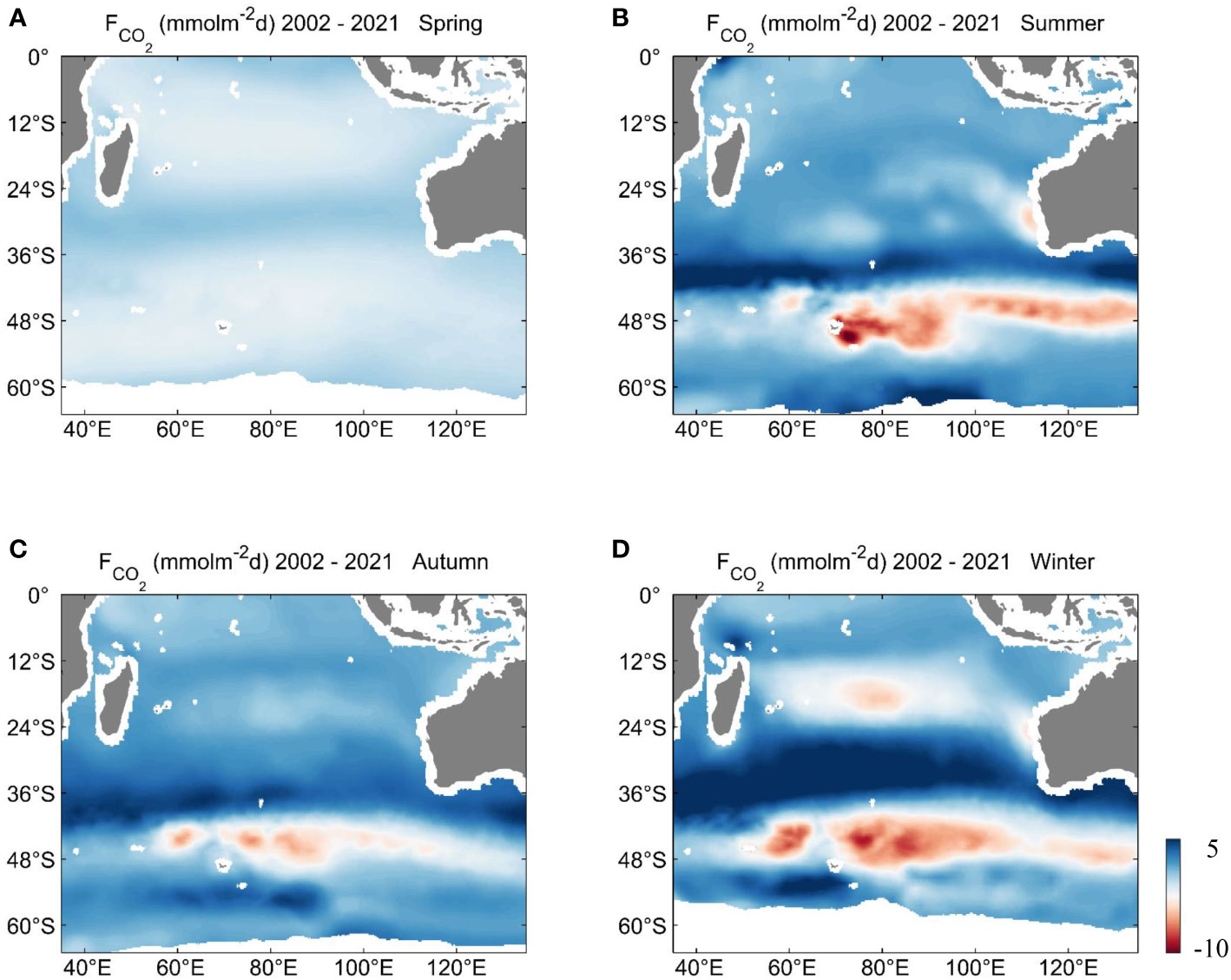
Figure 7 Differences for the seasonal and spatial distributions between with and without windseas impact. (A) Spring, (B) Summer, (C) Autumn, (D) Winter.

To further clarify the corresponding spatiotemporal relationships and reveal the long-term trend of air-sea CO₂ flux in the investigated two-decade time span, we show the zonal time series of air-sea CO₂ flux modulated by windseas for the entire Southern Indian Ocean in Figure 8. The overall pattern of CO₂ sources and sinks in the Southern Indian Ocean was relatively stable and had obvious temporal and spatial variations. In the tropical and subpolar regions, the Southern Indian Ocean was generally characterized by CO₂ sources with a weak interannual variation trend. The subtropical regions showed obvious seasonal variations, with sinks in winter and spring and sources in summer and autumn. The interannual variation remained unchanged in the 20-year time span included in this study. Obvious CO₂ source-to-sink and sink-to-source transition regions were found at approximately 25°S and 35°S, which was also consistent with observations (Jabaud-Jan et al., 2004; Xu et al., 2016; Lekshmi et al., 2021). The ACC region was a clear long-persisting CO₂ sink area, with increasing intensity of carbon absorption over time. We also found that approximately every seven years, a large CO₂ absorbing area formed, with effects covering 50 degrees of latitude from south to north. Each appearance of this area lasted for three years, and it contributed substantially to the net CO₂ uptake in the Southern Indian Ocean.

FIGURE 8

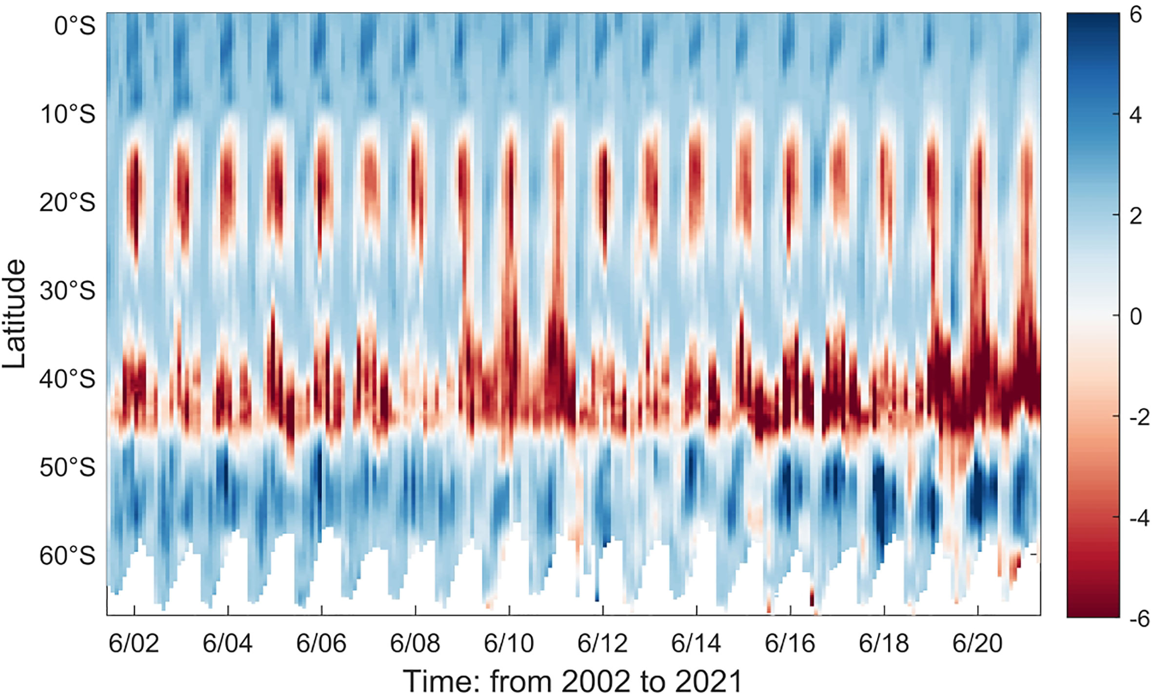
Figure 8 Zonal sequence diagram of F (mmol/m²·d) from 2002 to 2021 in the Southern Indian Ocean.

Figure 9 shows the 20-year zonal mean seasonal flux in the Southern Indian Ocean. To clearly highlight the impact of windseas on CO₂ exchange, we show the flux calculated from no waves in dashed lines and with waves in solid lines in this figure. Both the calculations from the two methods show clear spatiotemporal characteristics. In terms of spatial distribution, the CO₂ flux was less than or near to zero between 12°S and 48°S, which means this region is a CO₂ sink or saturation area. The CO₂ flux of all seasons was generally greater than or equal to zero between 0°S and 12°S, indicating a moderate CO₂ source. In contrast, although the CO₂ flux fluctuated significantly with the seasons at south of 48°S, the total CO₂ emissions were stronger. The sea area near the Antarctic continent mainly presented a weak convergence source and saturation zone. In terms of the seasonal distribution of air-sea CO₂ flux, the most dramatic fluctuations with latitude occurred in winter. The CO₂ uptake of the Southern Indian Ocean repeatedly increased and decreased, showing a “W” pattern covering form approximately 12°S to 48°S, with more CO₂ absorption in the middle and high latitudes than in the lower latitudes; the peak values of CO₂ absorption in winter were -3.23 mmol/m²·d with no waves and -3.31 mmol/m²·d with waves, reached at 38°S and 40°S, respectively. In spring and autumn, there was weak CO₂ absorption at north of 30°S, whereas the south was a strong CO₂ sink area. The maxima of CO₂ absorption with the impact of windseas were -2.21 mmol/m²·d and -4.48 mmol/m²·d respectively, reached at approximately 45°S. Overall, the Southern Indian Ocean had the strongest CO₂ uptake in summer, with seasonal mean absorption of approximately -1.97 mmol/m²·d under the influence of waves.

FIGURE 9

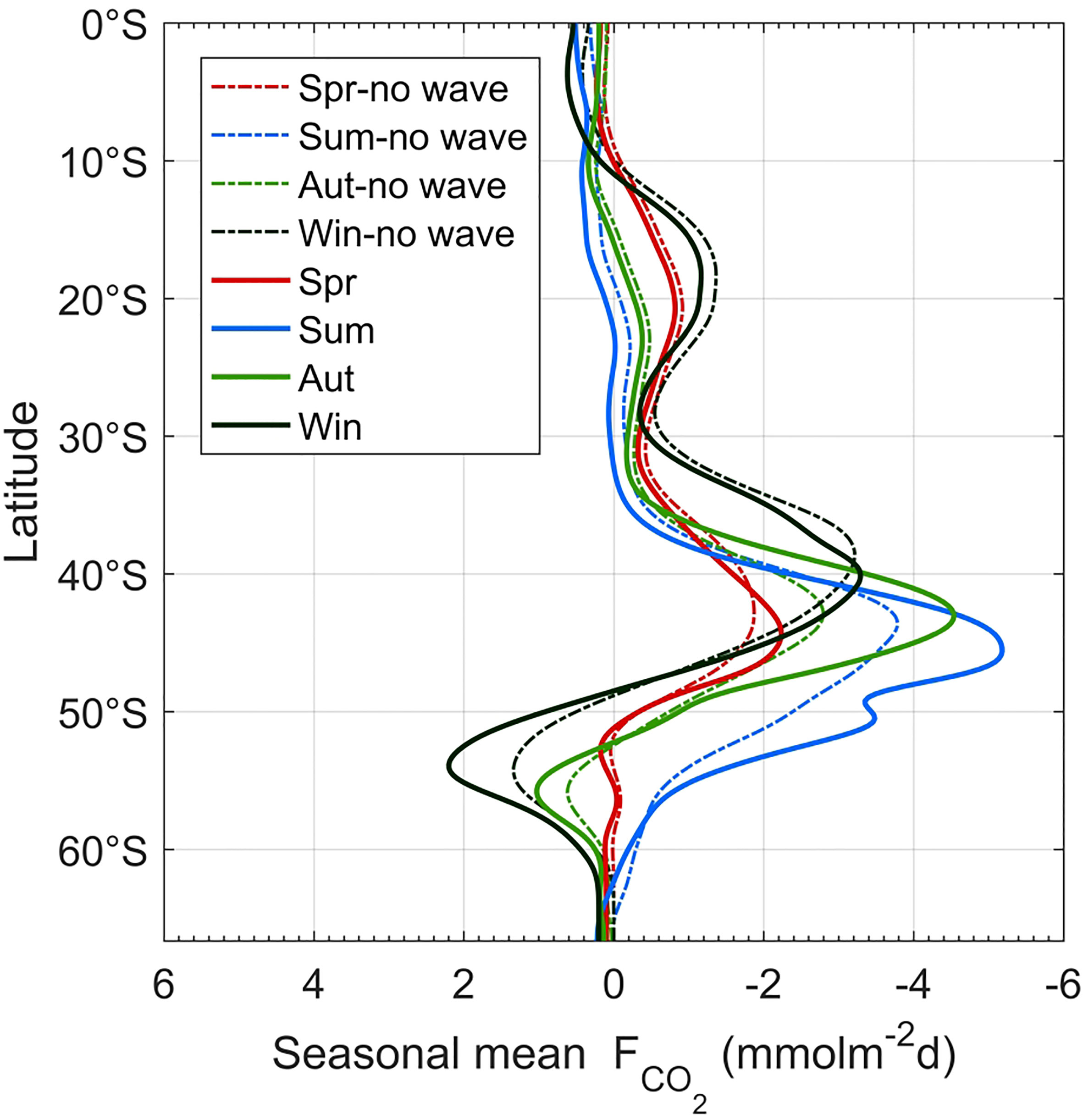
Figure 9 Seasonal mean zonal flux (mmol/m²·d) from 2002 to 2021 in the Southern Indian Ocean. Dashed lines are flux calculated with no waves and solid lines are calculated with waves.

3.3 Decadal CO₂ uptake trend predicted by the gas transfer velocity affected by windseas and no windseas

Finally, to further investigate the decadal CO₂ uptake trend and assess its important role in future carbon sequestration, we examined the seasonal evolution of air-sea net carbon flux (F_net) without the impact of waves in the Southern Indian Ocean from 2002 to 2021. We also present a time series of F_net with waves to evaluate the implications of the CO₂ uptake tread as affected by surface windseas (Figure 10). In each of these diagrams, the scattered points are seasonally averaged values integrated for the entire Southern Indian Ocean, and the lines are independent trends fitted for the corresponding seasons.

FIGURE 10

Figure 10 Evolution of air-sea net carbon flux, F_net(PgC) with waves and no waves in the Southern Indian Ocean. The scattered points are seasonally averaged values integrated for the entire Southern Indian Ocean, and the lines are independent trends fitted for the corresponding seasons.

In the last two decades, F_net was negative in all four seasons, which means that the Southern Indian Ocean is a perennial carbon sink. Among the different seasons, summer had the largest F_net, with an annual mean value without the influence of breaking waves of approximately -0.031 PgC. This was followed by winter, with an annual mean F_net of approximately -0.027 PgC, and then by spring and autumn, with annual mean values of -0.022 PgC and -0.021 PgC, respectively. The atmospheric CO₂ absorption capacity of the Southern Indian Ocean gradually strengthened over time. The fitting line between the F_net and time clearly shows a decreasing trend. In particular, the correlation shows a relatively smooth trend in the first decade but a much steeper trend in the second decade, which means that the sequestration of atmospheric carbon in the Southern Indian Ocean has become stronger in recent years. Again, summer had the most significant growth rate of F_net, with an annual rate of increase of approximately -0.000319 PgC/year with no waves. Under the impact of surface windseas, the annual mean F_net shows a clear increasing trend but has a stronger absorbing ability. The largest seasonal improvement is in summer, and the average result over the last 5 years is 32.12%. This indicates that surface wave breaking has a great impact on gas transfer velocity and hence total CO₂ uptake, especially in high wind speed seasons. Even in autumn, surface waves also clearly intensifies the total CO₂ uptake in the Southern Indian Ocean with an improvement of approximately 5.87%. Enter into the latest year, the capacity of CO₂ uptake in the Southern Indian Ocean reach a new peak in 2021. Especially in summer, annual mean value of F_net gets to approximately -0.048 PgC with the impact of windseas. These all suggest that a faster process of carbon sequestration is taking place in the Southern Indian Ocean.

4 Discussion and conclusion

Human-induced climate change has led to widespread disruption in nature and is affecting the lives and livelihoods of billions of people (IPCC, 2022a). Air-sea temperature change, sea level rise and extreme weather and climate events have become increasingly prominent due to excess emissions of greenhouse gases. The ocean is an important sink for anthropogenic CO₂ (Siegenthaler and Sarmiento, 1993). Studies have shown that the ocean absorbs more than 25% of the CO₂ emitted by human activities in the atmosphere (Watson et al., 2020) and therefore has a climate-change mitigating effect. The role of the ocean in regulating global climate is significantly affected by the spatiotemporal variation in CO₂ exchange processes at the ocean-atmosphere interface. Although significant importance of the world’s carbon cycle and mitigation of anthropogenic climate change, uncertainties remain in quantifying the global marine anthropogenic CO₂ sink as CO₂ uptake by the oceans fails to match emissions from human activities as atmospheric CO₂ levels increase (Khatiwala et al., 2013). At the same time, the ocean will also be negatively affected by climate warming and ocean acidification, further inhibiting its absorption of CO₂ or accelerating its release (Arias-Ortiz et al., 2018; Nakano and Iida, 2018; Aoki et al., 2021).

Surface waves consist of swells and windseas, which are two categories with completely different characteristic features. Previous studies using total waves to quantify the gas transfer velocity may overestimate the impact of waves on the overall CO₂ fluxes. In this study, we highlight the impact of windseas on the process of air-sea CO₂ exchange and address its important role in CO₂ uptake in the Southern Indian Ocean. The main findings of this study are as follows. In the Southern Indian Ocean, previous studies using total waves to modify the air-sea CO₂ transfer rate tended to overestimate the effect of waves. However, we found that windseas, as a main factor influencing gas transfer velocities, contributed only a small fraction of energy to the total waves in almost every region and seasons. Air-sea CO₂ flux showed strong spatiotemporal variation: Regarding seasonality in the Southern Indian Ocean, summer had the strongest CO₂ uptake capacity, with an annual mean flux of approximately −1.8 mmol/m²·d. The long-term seasonal variations in F_net in the Southern Indian Ocean are negative in all seasons, and the fitting correlations of F_net with time show a decreasing trend, which means that the sequestration of atmospheric carbon in the Southern Indian Ocean has been strengthening in recent years. This further indicates that the Southern Indian Ocean plays an increasingly important role in influencing global carbon cycling and constraining the global warming process. Meanwhile, the impact of surface waves clearly intensifies the total CO₂ uptake in the Southern Indian Ocean. Under the impact of surface windseas, the annual mean F_net shows a clear increasing trend but has a stronger absorbing ability. The largest improvement is in summer, with an average result over the last 5 years of 32.12%. Even in autumn, they have an improvement of approximately 5.87%.

This study presents new findings, but several limitations may still affect the quantitative parts of our results. As lack of direct field measurements of air-sea CO₂ flux, we cannot evaluate the impact of windseas proposed in this study, this is one of a major limitation of this work. Furthermore, we only calculated the CO₂ flux in the open ocean for lack of quantitative synthesis of integrated coastal ocean carbon, which may significantly underestimate the CO₂ uptake process in the entire Southern Indian Ocean. From a global perspective, even though coastal regions account for only 7%-8% of the global ocean area, such regions contribute approximately 28% of the total primary production and help to bury up to 80% of total organic carbon (Dai et al., 2022). Coastal regions are thus one of the most important carbon sinks in the world’s oceans and play a crucial role in mitigating global climate change. However, because of the lack of systematic observations and numerical simulations, accounting for these regions in global carbon cycle research remains challenging and has not yet been resolved in this study. In addition, we assumed that the process of ocean absorption of atmospheric CO₂ was solely controlled by certain physical factors. This obviously ignores potential interactions among different factors, such as wind speed, sea surface temperature, and salinity, which may have indirect effects on the CO₂ partial pressure at the surface. Several studies have also provided evidence that changes in SST, SSS, and wind speed can induce variations in the partial pressure of CO₂ via physicochemical processes that affect CO₂ exchange (Kashef-Haghighi and Ghoshal, 2013; Sun et al., 2021a; Sun et al., 2021b; Wanninkhof, 1992). We hope that necessary groundwork can be performed to address these problems in future research.

Data availability statement

The original contributions presented in the study are included in the article/supplementary material. Further inquiries can be directed to the corresponding authors.

Author contributions

JY, HZ, and HS conceptualized the research. KZ, JY, and HZ collected the data and contributed expertise to the construction and finalization of the manuscript. HS and KZ conducted the data processing and the main analysis and wrote the manuscript draft. HS and KZ share first authorship. All authors contributed to the article and approved the submitted version.

Funding

This research was financially supported by the National Natural Science Foundation of China (41976017, 42206014 and U20A2099), the Hainan Provincial Joint Project of Sanya Yazhou Bay Science and Technology City (220LH061) and Hainan Provincial Key Research and Development Projects (ZDYF2022SHFZ018).

Acknowledgments

AMSR data are produced by Remote Sensing Systems and were sponsored by the NASA AMSR-E Science Team and the NASA Earth Science MEaSUREs Program. Data are available at www.remss.com. NCEP Global Ocean Data Assimilation System (GODAS) data are provided by NOAA PSL, Boulder, Colorado, USA, from their website at https://psl.noaa.gov. The air-sea CO₂ partial pressure products are produced by NOAA National Centers for Environmental Information (DOI: https://doi.org/10.7289/V5Z899N6). The altimeter data in this study was obtained from Australian Ocean Data Network.

Conflict of interest

The authors declare that the research was conducted in the absence of any commercial or financial relationships that could be construed as a potential conflict of interest.

Publisher’s note

All claims expressed in this article are solely those of the authors and do not necessarily represent those of their affiliated organizations, or those of the publisher, the editors and the reviewers. Any product that may be evaluated in this article, or claim that may be made by its manufacturer, is not guaranteed or endorsed by the publisher.

References

Anoop T. R., Shanas P. R., Aboobacker V. M., Kumar V. S., Nair L. S., Prasad R., et al. (2020). On the generation and propagation of makran swells in the Arabian Sea. Int. J. Climatol. 40 (1), 585–593. doi: 10.1002/joc.6192