Ship-to-ship maritime wireless channel modeling under various sea state conditions based on REL model

The propagation of electromagnetic waves on land and sea is significantly different. Although the Los scenario is significant in marine wireless communication, the marine wireless channel exists an obvious two-ray phenomenon due to the strong reflection path reflected through the sea surface. By modeling the measured data of marine wireless channels, this paper calculates the radio propagation characteristics of the Pearl River estuary. In addition, the wave fluctuations and high humidity environment will also impact the properties of the marine wireless channel. Therefore, sea surface morphology models under multiple wind speeds are built. To estimate the path loss in the same area under different conditions, the Monte Carlo method is employed to quantify the results. The simulation results show that the electric wave propagation gradually degenerated from the round earth loss (REL) model to the free space model with increasing wind speed. Moreover, the distribution of the shadow fading varies with distance. The findings provide references for the network planning of marine communication.

1 Introduction

Space-air-ground-sea multiple access is an important key capability in the sixth generation (6G) network (Chen et al., 2022). 6G can achieve global seamless coverage, providing support for ultra-low latency (Li et al., 2021), digital twins, and other scenarios (Tang et al., 2022). However, the coverage of wide-band wireless signals on the ocean is still quite limited. Currently, maritime radio communication together with satellite and shore-based networks constitute part of maritime communication (Alqurashi et al., 2022). However, maritime conventional wireless communication systems mainly focus on the MF/HF/VHF bands, and satellite communication (Bekkadal, 2009) on the ocean provides wide coverage but high costs. Thus, the 3GPP Rel-16 (Lin et al., 2021) studied the non-terrestrial network (NTN) to support the 5G communication network and prepared for 6G technology. Therefore, marine communication is developing from traditional satellite communications to the marine NTN, and wide-band wireless communication will be expanded to ocean areas.

As the information is transferred via a medium in wireless communication, the properties of the wireless channel will determine the transmission rate and communication quality. Thus, it is essential to estimate the radio channel characteristics before network planning. Marine radio channel has special characteristics (Lees and Williamson, 2020). For example, in the terrestrial network, the fading is mainly relative to the relative position of the scatterers and the receiver, which exists in many Non-line-of-sight (NLoS) scenarios. Unlike that on the ground, the scatters on the sea surface are far less than that on the ground, but the radio channel varies with the ocean waves (Wang et al., 2018). What’s more, the sea surface is a random rough surface (Le Roux et al., 2009; Chen et al., 2021), so the research on sea surface radio channels generally belongs to the research of electromagnetic scattering from rough surfaces. Defer from the terrestrial environment, the real sea surface also has time-varying characteristics, and is affected by many factors such as wind speed, seabed topography, etc. That will generate propagation mechanism and multipath channel characteristics differed from other scenarios, which makes radio waves show unique loss and fading characteristics (Lees and Williamson, 2020). Therefore, the ocean wave’s impact on the marine radio channel is worth studying.

Therefore, the impact of changing ocean waves on a maritime radio channel still needs to be studied. The current paper aims to address this aspect and provides the maritime radio channel characteristics change with the ocean waves. In particular, this paper contributes the following aspects:

● The 5.9 GHz ship-to-ship radio channel measurement is conducted on the Pearl River estuary. With the introduction of equipment, a temporary point-to-point wireless communication network for maritime environments is built.

● Measured ship-to-ship path loss on the calm sea is extracted. We extract the path loss data from the measured data and verify the effectiveness of the round earth loss (REL) model. Results show that the REL model fits well with the measured data for a calm sea environment.

● Large scales fading characteristics for the maritime environment under various wind speeds are analyzed. The REL model and the PM wave spectrum model are used to model the propagation characteristics of the sea surface electromagnetic wave under different wind speeds. Based on the Monte Carlo method, the path loss and shadow fading characteristics of 5.9 GHz under the wind speed of 0-6m are quantitatively described.

The rest parts of this paper are organized as follows: Section 2 introduces the related works for maritime radio channel analysis. The description of the measurement campaign is given in Section 3. The measured path loss and its modeling are represented in Section 4. Sea surface morphology modeling is described in Section 5, while model verification and results analysis are provided in Section 6. Finally, the conclusion and discussion are drawn in Section 7.

2 Related works

Currently, empirical models for maritime radio rely primarily on measurement and statistical data (Habib and Moh, 2019). By making reasonable geometric assumptions (Huang et al., 2016), these models reduce the complex channel to a dual or multi-path path loss model. The reflection path from the sea surface is calculated using electromagnetic simulation or numerical analysis, with the roughness of the sea surface taken into account.

As far as the model of the offshore wireless channels is concerned, most of the current work focuses on the path loss model of different frequency bands (Maliatsos et al., 2006b; Maliatsos et al., 2006a). The sea surface radio channel model needs to consider the sea surface reflection phenomenon, so the Two-Ray model (Gaitán et al., 2020) was first used to model the sea wireless channel. The propagation loss measurement of the 5.8 GHz port WiMAX system carried out in Singapore Port confirms the effectiveness of the Two-Ray model (Joe et al., 2007), in which communication mode is from the land base station (BS) to the ship in the harbor of the WiMAX system. Moreover, the Influence of the tide and the shadow fading of obstacles on the sea surface could also be taken into account (Le Roux et al., 2009). The transmitter (TX) emitted signals of band 3.5 GHz and 5.8 GHz from the BS, while the receiver (RX) was fixed on the boat.

On basis of the Two-Ray model, the Plane Earth Loss (PEL) model (Saunders and Aragón-Zavala, 2007; Yee Hui et al., 2014) takes into account the reflection coefficients of electromagnetic waves on different media surfaces, which is widely used in cellular communications. However, as the distance between TX-RX gradually increases, when it reaches more than a few kilometers, the earth’s surface can no longer be assumed to be “flat”. Therefore, the curvature of the earth needs to be considered for long-distance wide ocean scenes (Yang et al., 2013). REL model (Gaitán et al., 2020) (Yu et al., 2017), divides the propagation area into two segments by the reflection point, and the path loss model considering the curvature of the earth is given. Under the premise of comprehensive consideration of the earth’s curvature and the reflection (Molisch, 2012), scattering (Saunders and Aragón-Zavala, 2007), diffraction (Reyes-Guerrero et al., 2011), and other propagation phenomena (Mabrouk et al., 2015; Alqurashi et al., 2022), together with environmental geometric analysis and measurement data, such as the diffuse reflection effect of rough surfaces could derive a novel path loss model. The effectiveness of this model has been verified by comparison with the Okumara-Hata, COST 231 (Singh, 2012), and ITU-R P.1546-2 models (Yang et al., 2019).

In our previous study (Yang et al., 2018; Li et al., 2021) and the papers mentioned above, the results were derived under calm sea conditions. However, the sea surface changes with the waves (Janssen, 2004). Ocean waves could cause shadow effects on electromagnetic reflective surfaces, the divergent effect of reflected signals, and the surface diffraction effect. Thus, we conducted a measurement to acquire the ship-to-ship radio channel data. Sea surfaces should also be modeled by leveraging the morphology methods. Then, the Monte Carlo method is used to quantify the results of estimating path loss in the same area under different conditions. This method is helpful to improve the generalization ability of the ocean surface channel model and provide accurate path loss under weather conditions that are difficult to measure.

3 Measurement Campaign

3.1 Equipment

To study the maritime radio channel characteristics, we conducted a ship-to-ship measurement in the Pearl River Estuary in Nansha, Guangzhou.

The TX part employed a Keysight signal source connected with a 5.9 GHz omnidirectional antenna (see Figure 1). The output gain of the amplifier was 40 dBm. The TX continuously transmitted chirp signals with a bandwidth of 1 MHz and a period of 2.56 ms. The equipment was both fixed on the TX and RX test boats. Meanwhile, the antenna was fixed at the highest point of the ship in both TX and RX, which is about 3 m from the sea surface. The RX part used a Keysight spectrum analyzer (see Figure 1). The spectrum analyzer was connected to a 5.9 GHz omnidirectional antenna via a low noise amplifier (LNA). We employed Matlab to control the spectrum analyzer to collect received signals, with a sampling frequency of 1 MHz. Similarly, the received antenna was fixed at the top of the boat, which was also 3 m high from the sea surface.

FIGURE 1

Figure 1 Overview of the equipment architecture.

The detailed parameters of the measurement system are listed in Table 1.

TABLE 1

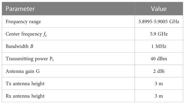
Table 1 System parameters.

3.2 Experiment

During the measurement, the sea surface was calm with a breeze of about 2 m/s (see Figure 2B). The experiment was conducted from 9 am-12 pm in the morning. The above figure shows the temperature and wind speed data of the area that day. During the experiment, the temperature was 30-31 °C (see Figure 2A, the wind direction was mainly south and southwest (see Figure 2C), the wind speed was small, and the sea was calm.

FIGURE 2

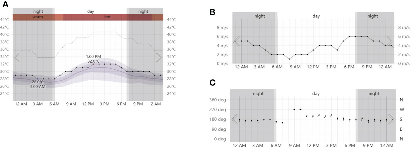
Figure 2 Weather conditions on the day of measurement: (A) is the temperature record; (B) is the wind speed record; and (C) is the wind direction record.

The measurement was carried out at the Pearl River estuary near the west side of Humen Bridge (shown in Figure 3). Nansha Marina served as the two ships’ departure point. Throughout the measurement, the TX moved in a small range near the shore, while the RX left the shore and moved about 3 km to the east. The RX boat’s average speed was around 10 km/h. The entire measurement procedure took approximately one hour. Figure 3 depicts the motion area of the two ships throughout the testing process.

FIGURE 3

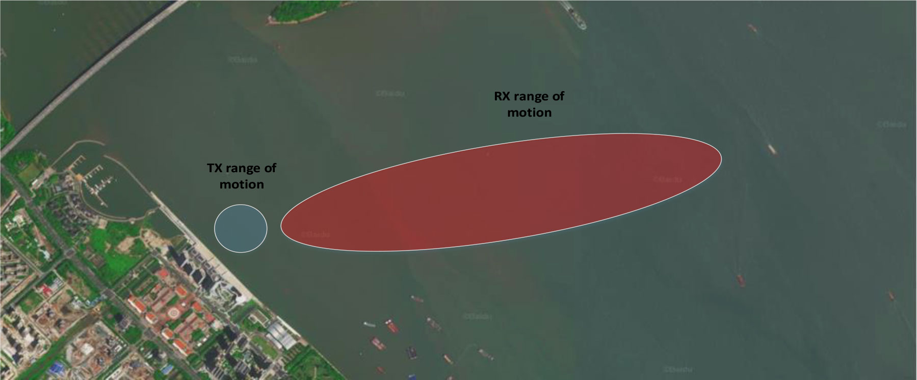
Figure 3 Satellite map of the measured area.

During the whole measurement process, the position with time stamps for both the TX and RX were recorded by the GPS. The TX continuously transmitted Chirp signals at 5.9 GHz. The Keysight spectrum analyzer on the RX boat was connected to a notebook that collected signals with the Matlab program, the notebook also recorded the time and GPS information of the collected signals. During the whole measurement process, about 200 groups of IQ data were collected by the spectrometer. The spectrum analyzer can sample 100000 times in a single acquisition, so each group of data includes 100000 IQ data. The collected IQ data can be used to analyze RX’s received energy information. Their time and position data were also obtained. The path loss model of the electromagnetic wave on the sea can be analyzed through the recorded position information of the TX and RX and the energy information of the received signal.

4 Modeling of measured path loss

4.1 REL model

According to the Two-Ray model and the actual measurement environment, it is stated in the paper (Yang et al., 2013) that when the TX-RX distance is large enough, the curvature of the earth cannot be ignored. Therefore, the Two-Ray model is modified by adding the curvature, as shown in Figure 4. Extending the Two-Ray model to the REL model allows more reliable channels for open scenes.

FIGURE 4

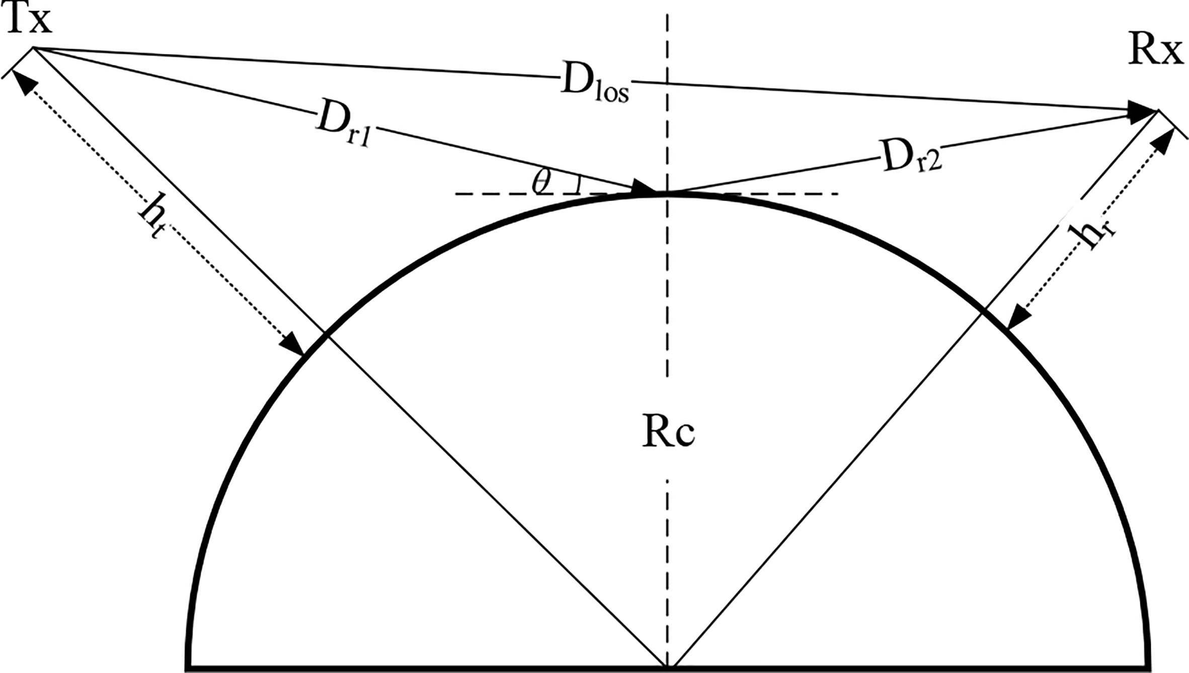
Figure 4 REL model.

In the REL model, the path loss is still consisted of the directed path and reflected path. As a result, the modified model also includes directed path loss and ground-reflected path loss. The model can be expressed by Formula (1), in which TX power is P_t and RX power is P_r.

$\begin{array}{ll}{L}_{\text{rel}}=-10{\log }_{10}\frac{P_{\text{r}}}{P_{\text{t}}}=20{\log }_{10}(\frac{\lambda }{4\pi D_{\text{LOS}}})+20{\log }_{10}\eta +L_{\text{e}\_\text{diff}}& (1)\end{array}$

$\begin{array}{ll}\eta =\left|1+R_{\text{rough}}·s_{\text{c}}·D_{\text{eff}}·e^{j\frac{2\pi }{\lambda }{D}_{\text{diff}}}\right|& (2)\end{array}$

where, η can be derived from Equation (2). R_rough represents effective reflection coefficient. s_c and D_eff express the shadowing and divergence coefficient, respectively. L_{e_diff} is the diffraction loss caused by the curvature of the earth (Yang et al., 2013).

4.2 Measured path loss

In this part, we will analyze the path loss characteristics of the sea surface based on the 200 signal data received. Through calibration in the laboratory, the corresponding relationship between the data recorded by the spectrum analyzer and the received energy can be obtained. And then the path loss can be calculated by combining the transmission power, transmission loss, transmission antenna gain, reception antenna gain, and reception loss.

From Figure 5 we can derive that the path loss for a calm sea surface fits well with the REL model, proving that the REL model is appropriate for ocean wideband radio propagation. In other words, the sea surface has specular electromagnetic wave reflection characteristics, since the calm sea surface is like a mirror. The measured path loss varies from 0 to 500 m and fluctuates significantly. Furthermore, the path loss increases significantly at 120 m, 180 m, and 360 m.

FIGURE 5

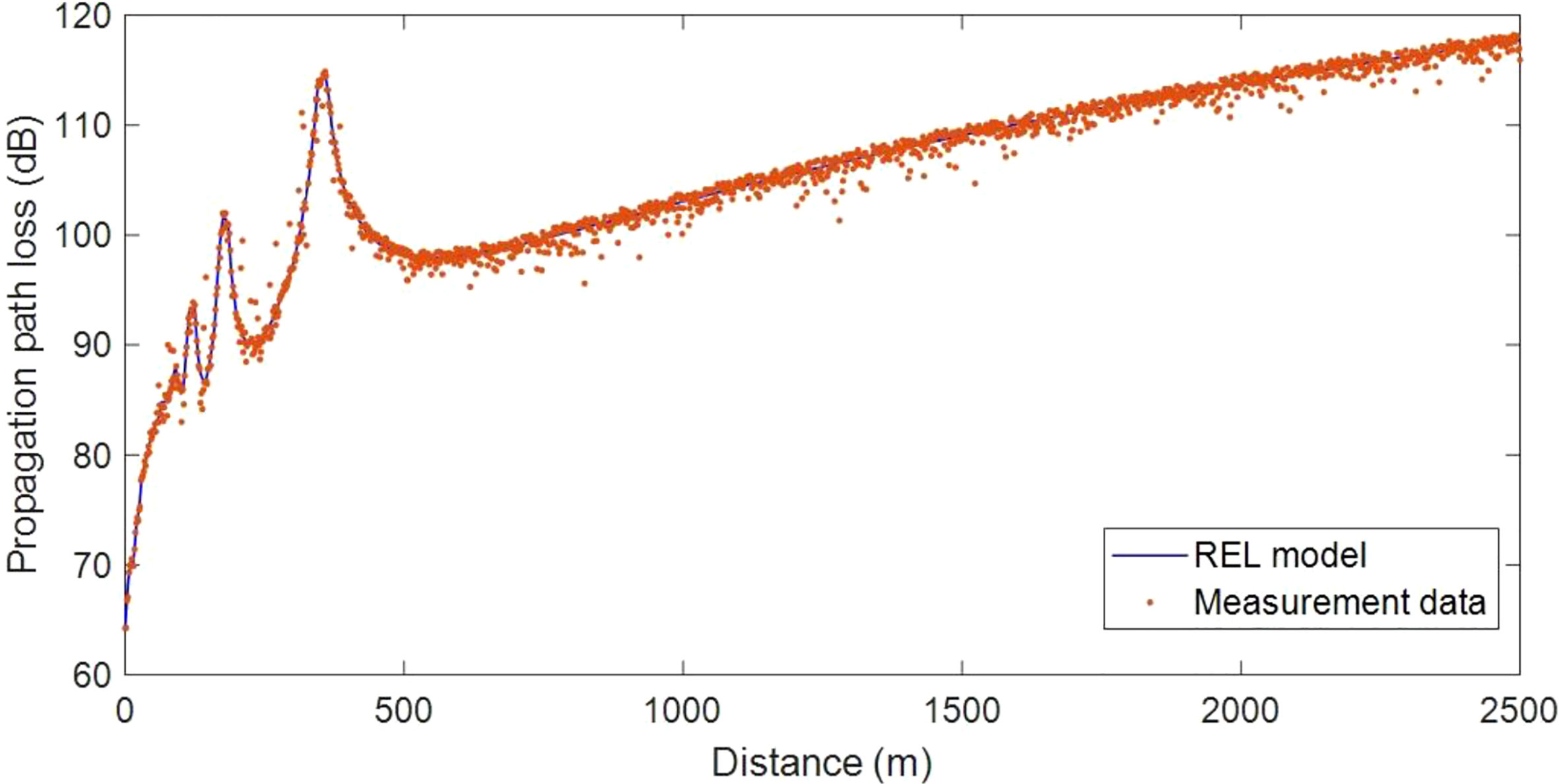
Figure 5 Measured propagation path loss compared with the REL model.

It is worth noting that as wind speed increases, ocean wave fluctuation will increase. As a result, the electromagnetic wave reflection point on the sea surface will change. Furthermore, the received power will vary. However, due to many limitations, including equipment conditions, safety considerations, and personnel scheduling factors, this paper did not obtain the measured channel path loss characteristics under a variety of complex sea conditions. As a result, to analyze the channel path loss characteristics under complex sea conditions, this paper combines the path loss model measured on the calm sea surface with the wave model under different wind speeds.

5 Sea surface morphology modeling

The aforementioned REL model is suitable for a calm sea. Nevertheless, the actual ocean wave fluctuation is extremely complex. It is formed by mixing waveforms with varying frequencies, wave heights, propagation directions, and phases. However, it is very complicated to use actual mathematical expressions to simulate waves (Peachey, 1986; Bhaskaran, 2019). Meanwhile, the wave theory of fluid mechanics is incapable of accurately predicting real-time variant ocean waves. Therefore, we simulate the ocean waves based on the wave spectrum and stochastic theory, to control the parameters in real-time simulation.

In a two-dimensional (2D) plane, ocean waves only consider the changes on the x-z axis. Because it does not involve the change of waves on the z-pane, the actual simulated results are only 2D wave curves that cannot adequately describe real-time ocean wave information. Ocean waves in three dimensions (3D) are studied by simulating them on the x-y axis at various angles to the z-axis. Thus, the ocean wave is made up of a variety of random phases, frequencies, and propagation directions. The following formula yields the 3D ocean wave (He et al., 2005).

$\begin{array}{ll}\text{ξ}(\text{x},\text{y},\text{t})={\sum }_{\text{i}=1}^{\text{m}}{\sum }_{\text{j}=1}^{\text{n}}{\text{A}}_{\text{n}}({\text{ω}}_{\text{i}},{\text{θ}}_{\text{j}})\text{cos}({\text{k}}_{\text{i}}{\text{xcosθ}}_{\text{j}}+{\text{k}}_{\text{i}}{\text{xsinθ}}_{\text{j}}-{\text{ω}}_{\text{i}}\text{t}+{\text{ϵ}}_{\text{ij}})& (3)\end{array}$

In the equation (4), A_n is the amplitude of multiple random waves which can be obtained by the following formula:

$\begin{array}{ll}{A}_{\text{n}}=\sqrt{2S(\omega ,\theta )\Delta \omega \Delta \theta }& (4)\end{array}$

k_i is the wave beam, and ε_ij is the random initial value phase subject to a uniform distribution. S(ω,θ) is the directional spectral function calculated by the following equation.

$\begin{array}{ll}S(\omega ,\theta )=S_{\text{n}}(\omega )G(\omega ,\theta )& (5)\end{array}$

where S_n(ω) is the frequency spectrum function, G(ω,θ) represents the directional function, ω is representative frequency, and θ is the phase that randomly selected in [0, 2π]. Different wave spectrum has different spectrum functions and orientation functions.

Here, we utilize Pierson Moscowitz (PM) spectrum (He et al., 2005) as the spectrum function for random wave generation. The PM spectrum is obtained by fitting the fully grown wave observation spectrum, which represents the fully grown wind waves. The spectral function of the PM spectrum is as follows:

$\begin{array}{ll}S(w)=\frac{a{g}^2}{w^5}exp(-\beta \frac{g^4}{U^5{w}^4})& (6)\end{array}$

where g is the gravitational acceleration, U is the wind speed at 19.5m from the sea surface, and a = 0.0081, β = 0.74. The sea surface morphology modeling results under different wind speeds by the aforementioned formulas (shown in Figure 6).

FIGURE 6

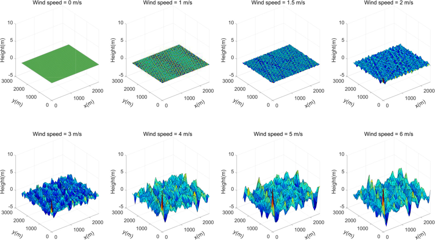
Figure 6 Simulated sea surface morphology under varying wind speed.

6 Results and analysis

6.1 Model verification

Figure 6 depicts the simulated sea surface morphology. To investigate the radio propagation mechanisms, the diagram shown in Figure 7 illustrates 4 types of ray propagation between TX and RX. We can see that there are no waves on the sea surface in Scenario 1. In this situation, the calm sea surface is like a mirror. The received signal comes from the directed path and reflected path. This is precisely the scenario we measured.

FIGURE 7

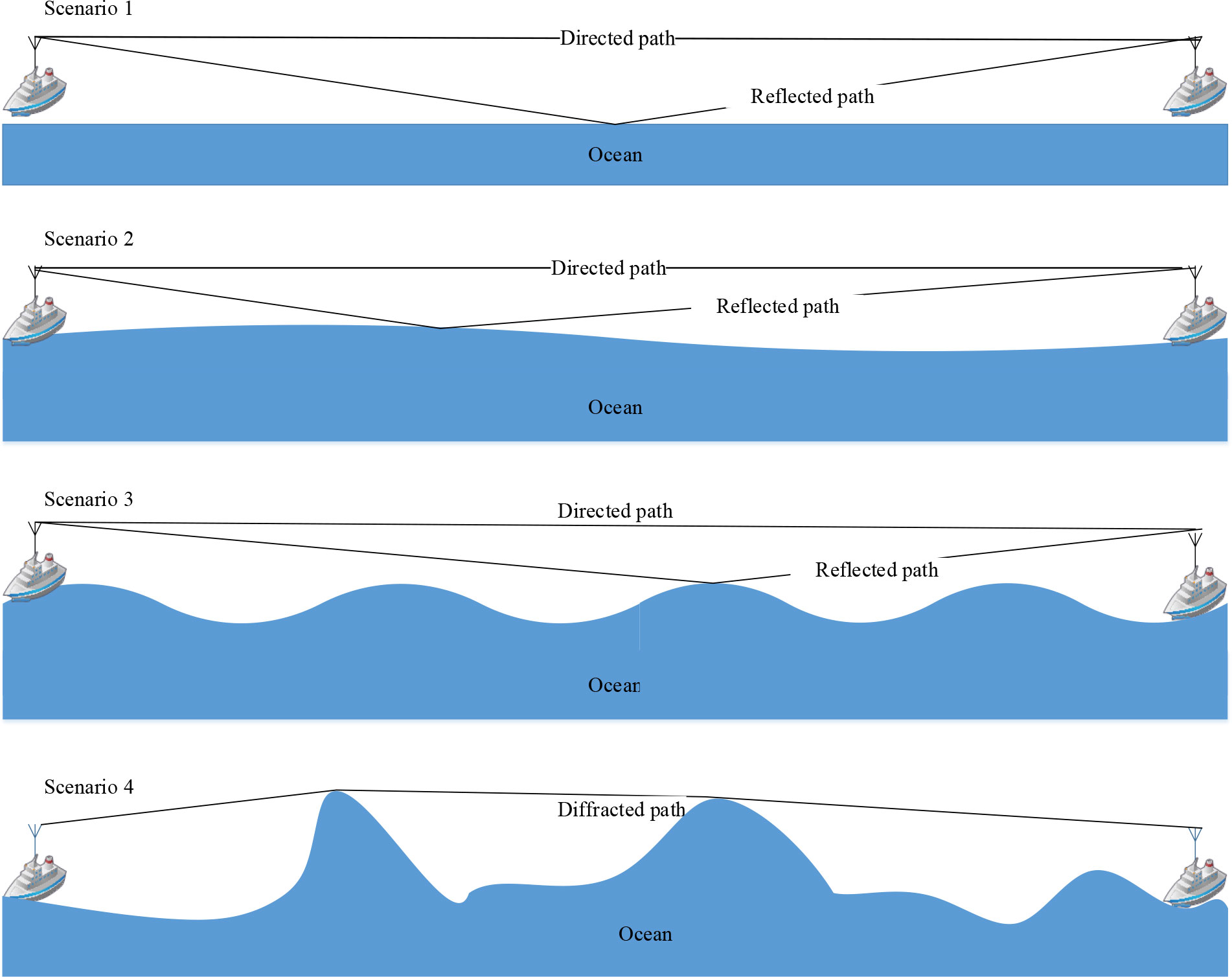
Figure 7 Radio propagation mechanisms under different sea surface conditions.

Although the sea surface cannot be completely calm in reality, its minor fluctuations are insufficient to change the position of the sea surface reflection signal over a wide range, so the measured electromagnetic wave path loss model in this scenario is very consistent with the REL model. The reflection point and height of the ship with the waves change as the ocean waves rise in Scenarios 2 and 3. Radio wave propagation characteristics will change due to interference between the straight path and the reflection path. Because the antenna height of the two communicating boats is low (only 3 m), the simulation indicates that electromagnetic waves may be blocked by the high ocean waves. Scenario 4 shows that there is only a diffracted path between TX and RX.

Therefore, to simulate the influence of random fluctuation of sea waves under different wind speeds on electromagnetic wave propagation on the sea surface, we use the Monte Carlo method (Hammersley, 2013) to simulate the path loss and shadow fading characteristics under different wind speeds.

The Monte Carlo method is also called the statistical simulation method, which is a numerical simulation method that takes probability phenomena as the research object. It is a method for calculating an unknown characteristic quantity by collecting statistical data through sampling. As a result, it can be used to calculate, simulate, and test discrete systems. The random characteristics of the system can be recreated in computational simulation by creating a probability model that closely matches the system performance and running random tests on a computer.

Firstly, the sea surface morphology needs to be modeled using the method mentioned in Section 5. We set the TX coordinate position on the sea surface area based on these simulated ocean surfaces. The REL model is then used to calculate the path loss at each of these points (see Figure 8). Following that, a large amount of data can be obtained. Using the extracted data, we analyze path loss and shadow fading. The detailed program is illustrated in Table 2.

FIGURE 8

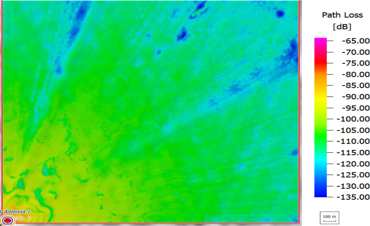
Figure 8 Energy hot map based on path loss.

TABLE 2

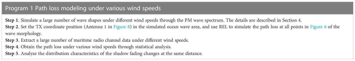
Table 2 Program of model verification.

6.2 Analysis

From Section 3.2, we can derive that the REL model fits well with the measured path loss. In this section, we use the REL model to calculate the path loss in the simulation. As shown in Figure 8, it is the sea surface path loss diagram using the REL model under the sea wave with 3 m/s wind speed, where the colors represent varying path loss values. In this paper, 50 figures of simulation data like Figure 8 are obtained under one wind speed, and 200 groups of path loss data can be obtained from each simulation data. Based on the large amount of data obtained, the characteristics of the sea channel are analyzed.

The TX is located at the lower left corner of the figure. The value of path loss from the TX to this point is represented by the color in the figure. A path loss curve can be formed by the value of the point where the ray from Antenna 1 passes. The figure shows that undulating waves cause significant differences in path loss curves in different directions. In this paper, we first obtain a large amount of morphological information about the sea surface (see Figure 6), then obtain the path loss as shown in Figure 8, and then extract a large number of path loss curves from Figure 8. Finally, we perform statistical analysis on these path loss curves to determine the path loss and shadow fading characteristics of the sea surface under wind speed.

The statistical curves of the sea surface path loss for different wind speeds obtained using the Monte Carlo method are shown in Figure 9. Each curve is based on the statistics of 10,000 sets of wave data under one wind speed simulation.

FIGURE 9

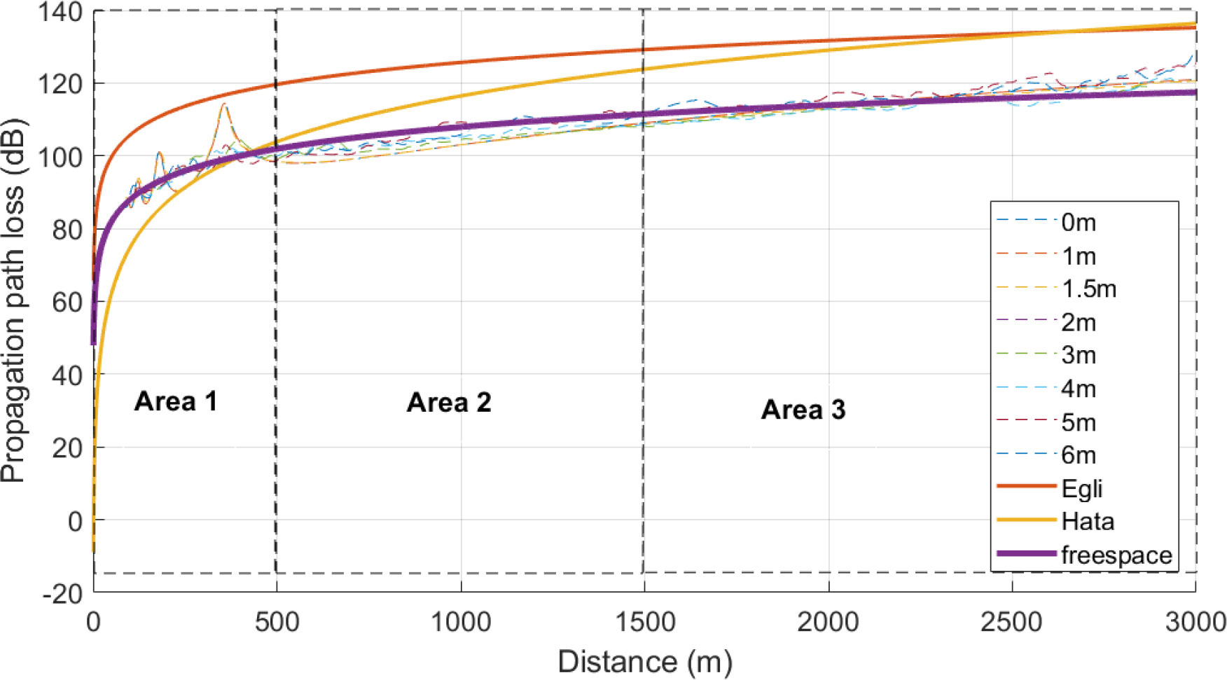
Figure 9 Simulated propagation path loss under various wind speeds.

The path loss under 0 m/s, 1 m/s, and 1.5 m/s waves are the same as that under a calm sea, indicating that the sea surface with wind speed less than 1.5 m/s belongs to a calm sea surface, and wave fluctuation has little influence on electromagnetic wave propagation. When the wind speed reaches 2 m/s, the two-ray phenomenon of the sea surface path loss characteristics disappears, which is mainly manifested in the fluctuation of the path loss value within the distance of 100 meters to 400 meters. Egli (Oluwole and Olajide, 2013), Hata (Emeruwa and Ekah, 2018), and Free Space models are employed in Figure 9. The path loss curve is consistent with the free space model. This shows that the deterministic interference between the LoS path and the reflection path caused by the reflection on the calm sea surface has become a random interference with the wave fluctuation, which causes the path loss model changes. At the same time, as the wave becomes strong due to the increased wind speed, it does not have a significant impact on long-distance propagation statistically, and the long-distance propagation model still conforms to the free space model.

Because of random wave fluctuation, the reflected and directed electromagnetic waves randomly overlap or block, resulting in the random change of the path loss from the transmitting side to the receiving side. The distribution of this change varies with the wave, which is associated with shadow fading and divergence. The distribution characteristics of shadow fading at different waves and distances at the sea surface are obtained by simulating the path loss characteristics of different waves at the same distance at a large number of source terminals.

In this paper, the distance is divided into three sections to analyze the shadow-fading effect. Figure 9 shows that two-path interference caused a significant change in path loss between 0 and 500 m. Thus, we make the 3 sections using Area 1/2/3. In Area 1 (0 - 500 m), the directed path and reflected path have obvious interference effects (5.9 GHz, receiver antenna height 3 m). Subsequently, the distance between 500 m to 2500 m is divided into two sections (Area 2 for 500 m -1500 m and Area 3 for > 1500 m). Interference and shadowing may occur as the distance between the directed and reflected paths increases.

Because the wave fluctuation has almost no impact on the sea surface morphology, under 0 m/s, 1 m/s, and 1.5m/s wind speed. Thus, we only consider the shadow fading under the wind speed of 2 m/s, 3 m/s, 4 m/s, 5 m/s, and 6 m/s.

To find the statistical regularity of the shadow fading, we analyze the cumulative distribution function (CDF) for three distance ranges.

Figure 10 depicts the CDF of the shadow fading distribution of Area 1, ranging from about -13.5 dB to about 15.5 dB because 0-500m is the obvious region of the REL benefit. The 10% CDF is - 7.18 dB, the 50% CDF is about 0 dB, and the 90% CDF is 8.42 dB. Table 3 contains the specifics. The CDF varies slightly depending on the ocean wave, and when the wind speed is low, the dispersion range of shadow fading is slightly larger. This is because the range of 0 - 500 m is located in the interference area of the directed and reflected path. Meanwhile, the interference effect change with the wave fluctuation.

FIGURE 10

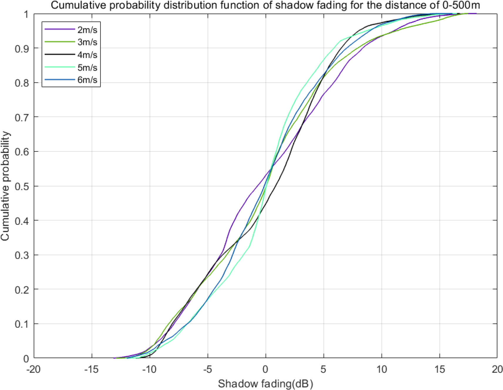
Figure 10 CDF of the shadow fading for Area 1.

TABLE 3

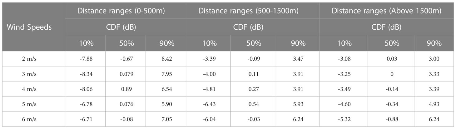
Table 3 Statistic results.

Figure 11 shows the CDF of the shadow fading distribution of the RX at a distance of 500-1500 m. It can be seen from the figure that with the increase of the wind speed, the distribution range of the shadow fading expands significantly. The specific distribution values of shadow fading are shown in Table 3. As the wind speed increases from 2 m/s to 6 m/s, 10% of CDF changes from -3.39 dB to -6.04 dB, and 90% of CDF changes from 3.47 dB to 6.24 dB. The simulation shows that wind-induced wave fluctuation significantly impacts the shadow fading of radio wave propagation on the sea surface.

FIGURE 11

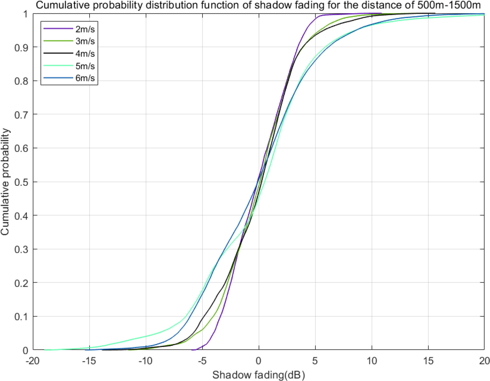
Figure 11 CDF of the shadow fading for Area 2.

Figure 12 shows the CDF of the shadow fading distribution of the receiving end at a distance longer than 1500 m. An obvious trend can still be seen in Figure 12, which is similar to what is displayed in Figure 11. With the increase of the wind speed, the distribution range of the shadow fading becomes significantly larger. As the wind speed changes from 2 m/s to 6 m/s, 10% of CDF changes from -3.08 dB to -5.32 dB, and 90% of CDF changes from 3 dB to 6.24 dB. It can also be observed from the table that the distribution range of shadow fading is slightly less than 500 m-1500 m when the distance is larger than 1500 m.

FIGURE 12

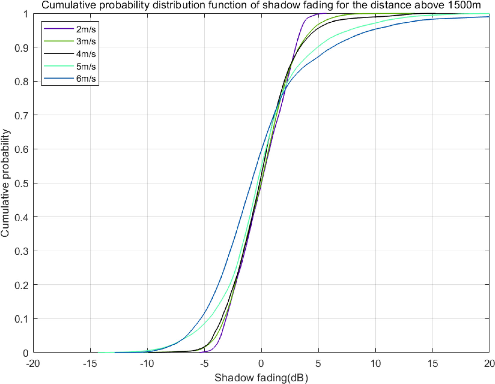
Figure 12 CDF of the shadow fading for Area 3.

7 Conclusions and discussions

This paper begins by describing a channel measurement activity that we conducted at sea. And then the paper introduces the REL model for sea surface propagation and based on the measured data, it is observed that the propagation characteristics of electromagnetic waves on the calm sea surface fit the REL model. Because obtaining channel test data under severe weather is difficult, this paper employs the Monte Carlo method to simulate path loss and shadow fading characteristics in different waves generated by the PM wave spectrum model. The simulation results show that as the wind speed on the sea increases, the radio wave propagation model transitions from the REL model to the Free Space model. The general trend of the shadow fading characteristics is that the distribution gradually widens as the sea waves grow larger.

The simulation results in this paper show that the wave fluctuation caused by the rising wind speed will weaken the two-path effect on the sea surface, which will make the originally large path loss at some distance smaller, which is conducive to communication, but at the same time, the simulation also shows that the wave will increase the impact of shadow fading on the sea surface, resulting in energy fluctuation, which will affect the performance of the receiver. The findings of our study can serve as a guide for the development of maritime 5G mobile communication networks under complex sea conditions.

Data availability statement

The original contributions presented in the study are included in the article/supplementary material. Further inquiries can be directed to the corresponding author.

Author contributions

FL: conceptualization, resources, methodology, software, validation, formal analysis, writing—original draft. YS: conceptualization, measurement, writing—review & editing. JL: measurement, software. KY: conceptualization, writing—review & editing. JY: writing—review & editing. All authors contributed to the article and approved the submitted version.

Funding

The study is supported by the Natural Science Foundation of Hubei Province [2022CFB285], and partly supported by the 2022 Scientific Research Program of the Hubei Provincial Department of Education [No. B2022391], the discipline construction project of Transportation Engineering of Guangzhou Jiaotong University, and Basic Scientific Research Fund of Zhejiang Provincial Universities under Grant No. 2021JD004.

Acknowledgments

This project would have been impossible without the support of Guangzhou Maritime University. The authors would also like to thank my colleagues for their wonderful collaboration.

Conflict of interest

JY is employed by Beijing Metaradio Technologies Co., Ltd.

The remaining authors declare that the research was conducted in the absence of any commercial or financial relationships that could be construed as a potential conflict of interest.

Publisher’s note

All claims expressed in this article are solely those of the authors and do not necessarily represent those of their affiliated organizations, or those of the publisher, the editors and the reviewers. Any product that may be evaluated in this article, or claim that may be made by its manufacturer, is not guaranteed or endorsed by the publisher.

References

Alqurashi F. S., Trichili A., Saeed N., Ooi B. S., Alouini M. S. (2022). Maritime communications: a survey on enabling technologies, opportunities, and challenges. IEEE Internet Things J. 10 (4), 3525–3547. doi: 10.1109/JIOT.2022.3219674

CrossRef Full Text | Google Scholar

Bekkadal F. (2009). “Emerging maritime communications technologies,” in 2009 9th International Conference on Intelligent Transport Systems Telecommunications, (ITST), Lille, France. 358–363. doi: 10.1109/ITST.2009.5399329

CrossRef Full Text | Google Scholar

Bhaskaran P. K. (2019). Challenges and future directions in ocean wave modeling - a review. J. Extreme Events 6 (02), 1950004. doi: 10.1142/S2345737619500040

CrossRef Full Text | Google Scholar

Chen W., Li C., Yu J., Zhang J., Chang F. (2021). A survey of maritime communications: From the wireless channel measurements and modeling perspective. Regional Stud. Mar. Sci. 48, 102031. doi: 10.1016/j.rsma.2021.102031

CrossRef Full Text | Google Scholar

Chen W., Montojo J., Lee J., Shafi M., Kim Y. (2022). The standardization of 5G-advanced in 3GPP. IEEE Commun. Magazine 60 (11), 98–104. doi: 10.1109/MCOM.005.2200074

CrossRef Full Text | Google Scholar

Emeruwa C., Ekah U. J. (2018). Pathloss model evaluation for long term evolution in owerri. Int. J. Innovative Sci. Res. Technol. 3 (11), 491–496.

Google Scholar

Gaitán M. G., Santos P. M., Pinto L. R., Almeida L. (2020). “Experimental evaluation of the two-ray model for near-shore WiFi-based network systems design,” in 2020 IEEE 91st Vehicular Technology Conference (VTC2020-Spring) Handbook for Marine Radio Communication, Publisher name: Informa Law from Routledge. 1–3. doi: 10.4324/9781315766393

CrossRef Full Text | Google Scholar

Habib A., Moh S. (2019). Wireless channel models for over-the-sea communication: A comparative study. Appl. Sci. 9 (3), 443. doi: 10.3390/app9030443

CrossRef Full Text | Google Scholar

Hammersley J. (2013). Monte Carlo methods (London, United Kingdom: CHAPMAN AND HALL). doi: 10.1007/978-94-009-5819-7

CrossRef Full Text | Google Scholar

He H., Liu H., Zeng F., Yang G. (2005). “A way to real-time ocean wave simulation,” in International Conference on Computer Graphics, Imaging and Visualization (CGIV'05), Beijing, China, 409–415. doi: 10.1109/CGIV.2005.11

CrossRef Full Text | Google Scholar

Huang F., Liao X., Bai Y. (2016). Multipath channel model for radio propagation over sea surface. Wireless Pers. Commun. 90 (1), 245–257. doi: 10.1007/s11277-016-3343-4

CrossRef Full Text | Google Scholar

Janssen P. (2004). The interaction of ocean waves and wind (Cambridge, United Kingdom: Cambridge University Press).

Google Scholar

Joe J., Hazra S. K., Toh S. H., Tan W. M., Shankar J., Hoang V. D., et al. (2007). “Path loss measurements in sea port for WiMAX,” in 2007 IEEE Wireless Communications and Networking Conference, Hong Kong, China., 1871–1876. doi: 10.1109/WCNC.2007.351

CrossRef Full Text | Google Scholar

Lees G. D., Williamson W. G. (2020). Handbook for marine radio communication (London, United Kingdom: Informa Law from Routledge). doi: 10.4324/9781315766393

CrossRef Full Text | Google Scholar

Le Roux Y. M., Ménard J., Toquin C., Jolivet J. P., Nicolas F. (2009). “Experimental measurements of propagation characteristics for maritime radio links,” in 2009 9th International Conference on Intelligent Transport Systems Telecommunications,(ITST), Lille, France., 364–369. doi: 10.1109/ITST.2009.5399326

CrossRef Full Text | Google Scholar

Li C., Yu J., Xue J., Chen W., Wang S., Yang K. (2021). Maritime broadband communication: Wireless channel measurement and characteristic analysis for offshore waters. J. Mar. Sci. Eng. 9 (7), 783. doi: 10.3390/jmse9070783

CrossRef Full Text | Google Scholar

Li Z., Zhu N., Wu D., Wang H., Wang R. (2021). Energy-efficient mobile edge computing under delay constraints. IEEE Trans. Green Commun. Networking 6 (2), 776–786. doi: 10.1109/TGCN.2021.3138729

CrossRef Full Text | Google Scholar

Lin X., Rommer S., Euler S., Yavuz E. A., Karlsson R. S. (2021). 5G from space: An overview of 3GPP non-terrestrial networks. IEEE Commun. Standards Magazine 5, (4), 147–153. doi: 10.1109/MCOMSTD.011.2100038

CrossRef Full Text | Google Scholar

Mabrouk I. B., Reyes-Guerrero J. C., Nedil M. (2015). “Radio-channel characterization of an over-sea communication,” in 2015 9th European Conference on Antennas and Propagation (EuCAP), Lisbon, Portugal., 1–4.

Google Scholar

Maliatsos K., Constantinou P., Dallas P., Ikonomou M. (2006a). “Measuring and modeling the wideband mobile channel for above the sea propagation paths,” in 2006 First European Conference on Antennas and Propagation, Nice, France., 1–6. doi: 10.1109/EUCAP.2006.4584755

CrossRef Full Text | Google Scholar

Maliatsos K., Loulis P., Chronopoulos M., Constantinou P., Dallas P., Ikonomou M. (2006b). “Measurements and wideband channel characterization for over-the-sea propagation,” in 2006 IEEE International Conference on Wireless and Mobile Computing, Networking and Communications, Montreal, QC, Canada., 237–244. doi: 10.1109/WIMOB.2006.1696376

CrossRef Full Text | Google Scholar

Molisch A. F. (2012). Wireless communications (The Atrium, Southern Gate, Chichester, West Sussex, United Kingdom: John Wiley & Sons).

Google Scholar

Oluwole F. J., Olajide O. Y. (2013). Radio frequency propagation mechanisms and empirical models for hilly areas. Int. J. Electrical Comput. Eng. (IJECE) 3 (3), 372–376. doi: 10.11591/ijece.v3i3.2519

CrossRef Full Text | Google Scholar

Peachey D. R. (1986). Modeling waves and surf. ACM Siggraph Comput. Graphics 20 (4), 65–74. doi: 10.1145/15886.15893

CrossRef Full Text | Google Scholar

Reyes-Guerrero J. C., Bruno M., Mariscal L. A., Medouri A. (2011). “Buoy-to-ship experimental measurements over sea at 5.8 GHz near urban environments,” in 2011 11th Mediterranean Microwave Symposium (MMS), Yasmine Hammamet, Tunisia., 320–324. doi: 10.1109/MMS.2011.6068590

CrossRef Full Text | Google Scholar

Saunders S. R., Aragón-Zavala A. (2007). Antennas and propagation for wireless communication systems (The Atrium, Southern Gate, Chichester, West Sussex, United Kingdom: John Wiley & Sons).

Google Scholar

Singh Y. (2012). Comparison of okumura, hata and cost-231 models on the basis of path loss and signal strength. Int. J. Comput. Appl. 59 (11), 37–41. doi: 10.5120/9594-4216

CrossRef Full Text | Google Scholar

Tang T., Li L., Wu X., Chen R., Li H., Lu G., et al. (2022). TSA-SCC: text semantic-aware screen content coding with ultra low bitrate. IEEE Trans. Image Process. 31, 2463–2477. doi: 10.1109/TIP.2022.3152003

PubMed Abstract | CrossRef Full Text | Google Scholar

Wang J., Zhou H., Li Y., Sun Q., Wu Y., Jin S., et al. (2018). Wireless channel models for maritime communications. IEEE Access 6, 68070–68088. doi: 10.1109/ACCESS.2018.2879902

CrossRef Full Text | Google Scholar

Yang K., Molisch A. F., Ekman T., Røste T., Berbineau M. (2019). A round earth loss model and small-scale channel properties for open-sea radio propagation. IEEE Trans. Vehicular Technol. 68 (9), 8449–8460. doi: 10.1109/TVT.2019.2929914

CrossRef Full Text | Google Scholar

Yang K., Molisch A. F., Ekman T., Roste T. (2013). “A deterministic round earth loss model for open-sea radio propagation,” in 2013 IEEE 77th Vehicular Technology Conference (VTC Spring), Dresden, Germany., 1–5. doi: 10.1109/VTCSpring.2013.6691821

CrossRef Full Text | Google Scholar

Yang K., Zhou N., Røste T., Eide E., Ekman T., Hasfjord A. M., et al. (2018). “Wifi measurement for the autonomous boat’DRONE 1’in Trondheim fjord,” in The 1st International Conference on Maritime Autonomous Surface Ship (ICMASS 2018), Busan, Korea.

Google Scholar

Yee Hui L. E. E., Dong F., Meng Y. S. (2014). Near sea-surface mobile radiowave propagation at 5 GHz: measurements and modeling. Radioengineering 23 (3), 824–830.

Google Scholar

Yu J., Chen W., Yang K., Li C., Li F., Shui Y. (2017). Path loss channel model for inland river radio propagation at 1.4 GHz. Int. J. Antennas Propagation 2017, 1–15. doi: 10.1155/2017/5853724

CrossRef Full Text | Google Scholar