Wide-area sound speed profile estimation based on a pre-classification scheme for sound speed perturbation modes

Introduction: The trend of sound speed profile (SSP) inversion is towards wide-area sound speed estimation. However, the traditional inversion method of dividing the latitude and longitude grids has limitations in terms of significantly lower accuracy when samples are lacking. k-means clustering algorithm (K-means) can divide the training class to achieve high accuracy estimation.

Method: This paper proposes a grid-free pre-classification inversion scheme based on empirical orthogonal function (EOF) vectors. The scheme is based on the K-means to classify the samples according to the perturbation mode of the SSP. After classification, the SSP inversion is carried out using the self-organizing map algorithm (SOM). The experimental sea area is selected from the South China Sea, and the inversion results are evaluated using root mean square error (RMSE) as the criterion.

Result: The inversion results show that the inversion error is 2.1 m/s for the pre-classification solution and 2.7 m/s for the solution without pre-classification, a steady improvement of more than 20% in the inversion error. Accuracy is also improved by 2.14 m/s in the depth range where the sound speed perturbance is greatest.

Discussion: This pre-classification scheme has smaller inversion errors and the classification results are reasonable in terms of distribution in time and space. It provides a feasible solution for SSP inversion in sea areas where samples are lacking.

1 Introduction

Sound speed profiles (SSP) are an important dynamic factor influencing underwater acoustic energy, and their acquisition in real-time is of great importance for sound propagation (Stojanovic et al., 1994; Rouseff et al., 2001; Song, 2017; Han and Yao, 2021; Li et al., 2022b). However, SSP measurements have a broad spatial and temporal coverage, and obtaining SSP through in situ measurements is time-consuming. On the other hand, the satellite remote sensing platform has comprehensive coverage and real-time characteristics, which can meet the observation needs of SSP measurement with wide spatial and temporal coverage. Still, the data it acquires are limited to the sea surface. Therefore, the research focuses on using certain physical relationships to project the satellite acquired sea surface information downward to estimate the underwater sound speed in real time (LeBlond, 1976). There have been two approaches to reconstructing the underwater data using sea surface data for a long time. One is the traditional model of the physical relationship between the sea surface and the underwater field. Carnes estimated underwater profile data for the NW Pacific and NW Atlantic using empirical orthogonal and single empirical orthogonal regression functions (Carnes et al., 1994). The US Navy later included this inversion method as part of its operational marine environment prediction program due to its good performance in terms of efficiency and accuracy (Chu et al., 2004). Since then, the multivariate projection method proposed by Fischer (2000) and the multivariate regression method proposed by Nardelli and Santoleri (2004) have also been successful in acquiring underwater structures. However, these traditional methods are mainly based on a linear relationship between the surface and subsurface (Meijers et al., 2011). Their performance deteriorates in sea areas with complex sea conditions due to the highly non-linear nature of the ocean. So, another class of machine methods with the advantage of extracting non-linear relationships from a data set is gradually being used in this field (Liu and Weisberg, 2005; Jain and Ali, 2006; Li et al., 2022a). In recent years, Su used the XGBoost model to reconstruct the global underwater thermohaline structure (Su et al., 2019), and Chen used the self-organizing map (SOM) to reconstruct the underwater temperature data in the Kuroshio extension of the Pacific Ocean east of the island of Japan (Chen et al., 2020). Ou used the Random Forest algorithm to reconstruct the underwater sound speed data in the South China Sea (Ou et al., 2022a). Bao et al. estimated Pacific subsurface salinity data using a generalized regression neural network FOAGRNN model with a fruit fly optimization algorithm (Bao et al., 2019). An increasing number of machine learning algorithms are being used in this area, and most show better performance (Charantonis et al., 2015; Bianco and Gerstoft, 2017; Li et al., 2022d; Li et al., 2022c).

Machine learning is efficient and high performing, but it also faces apparent problems. One of the most realistic problems is that machine learning algorithms require many samples as a training set to get a good estimation result. Insufficient samples in the training set can directly lead to wrong estimation results (Frederick et al., 2020). If the time series and spatial orientation were expanded to introduce more samples, this would lead to inconsistent basis functions for the inversions and introduce more significant errors due to differences in the perturbation mechanisms. To maintain the consistency of the basic functions, the traditional treatment is to divide the sea area into individual 1° x 1° or 2° x 2° latitude and longitude grid cells and then extract the Empirical orthogonal function (EOF) vector basis functions in each grid (Chen et al., 2018; Li et al., 2021). When the sample data is insufficient, the whole sea area is treated as a large grid in a unified manner. This treatment will result in greater errors due to the large area of the sea grid and differences in the sound speed perturbation mechanisms in the sea area, resulting in inconsistencies in the derived basis functions. This paper proposes a pre-classification scheme based on the extraction of EOF vectors from sound speed profiles to solve the difficulty of the above machine learning algorithm to divide the grid in the sea with insufficient data samples. This scheme classifies sea areas with similar perturbance mechanisms into the same class of data samples. The classification is based on the consistency of the EOF basis functions tested using the K-means algorithm. The SSP is inverted using the SOM algorithm after the classification. The K-means algorithm is a classical Euclidean distance-based clustering algorithm that can reasonably classify seas based on the similarity of EOF. Previous scholars have applied it to the estimation of thermohaline profiles showing that this classification algorithm is feasible and effective (Hjelmervik and Hjelmervik, 2013). The SOM algorithm can fuse the input SSP inversion-related parameters by simulating a lateral inhibition phenomenon in the biological nervous system; similar inversions by previous scholars using the SOM have also shown good performance (Chapman and Charantonis, 2017).

The experimental area was selected from the South China Sea, the largest marginal sea connecting the Indian and Pacific Oceans. Its unique semi-enclosed basin structure, monsoons, and other factors led to a complex SSP distribution and perturbation, which presented a challenge to the SSP inversion scheme (Sun et al., 2020). The most critical difficulty is that due to political and economic reasons, Argo buoys are sparsely deployed in the South China Sea region, and SSP samples are scarce in the South China Sea compared to other water areas. This makes it challenging to implement inversion solutions for relevant machine learning algorithms. Therefore, the pre-classification scheme in this paper was chosen to conduct experiments in the South China Sea, which can verify the validity and feasibility of the classification scheme. The classification divides the sea area into three types of samples, and the results of the inversion experiments are evaluated for the assessment using root mean square error (RMSE). The inversion results show an accuracy of 2.1 m/s after pre-classification treatment of the South China Sea. The inversion accuracy using the traditional treatment of the entire South China Sea as one large grid is 2.7 m/s. The pre-classification scheme improves the inversion accuracy by 0.6 m/s and stabilizes upgrading the inversion accuracy by more than 20%. The experimental results show that using the K-means algorithm to check the consistency of the empirical orthogonal function and to pre-classify the sea area is an effective solution for the difficulty of dividing the training grid of machine learning algorithms into complex sea areas with insufficient data samples. It achieves a high accuracy inversion of the de-gridded SSP for complex sea areas with insufficient data samples.

2 Data

Three main types of data were used in this experiment: Argo buoy data, satellite remote sensing data, and World Ocean Atlas 2018 (WOA18) data.

2.1 Satellite remote sensing data

The satellite remote sensing data used in the study are sea surface temperature anomaly (SSTA) and sea level anomalies (SLA). SSTA and SLA data from the Copernicus Project (https://marine.copernicus.eu/). The temporal resolution was chosen as one day, and the spatial resolution was chosen as 0.25° × 0.25°.

2.2 Background profile data

The background profiles are taken from the WOA18 dataset, derived from the National Oceanic Data Research Center (NODC) climate state ocean hydrographic data (https://www.ncei.noaa.gov/products/world-ocean-atlas). It is a climate-averaged data set that integrates temperature, salinity, density, and other data sets and measurements from various global seas, including annual, seasonal, and monthly averages. It is generally available at 0.25°, 1°, and 5° spatial resolution. The WOA18 data used in this experiment were selected as annual averages for 2005-2017, with a spatial resolution of 0.25° × 0.25°.

2.3 Argo data

The international Argo program was implemented in 2000, with over 15000 automated profiling buoys deployed in the global ocean by many countries. This was mainly for measuring temperature and salinity profiles. The Argo data used in the experiments were taken from the Global Ocean Argo Scattered Data Collection by the China Argo Reference Centre (ftp://ftp.argo.org.cn/pub/ARGO/global). Due to political and sea complexity factors, buoys in the South China Sea are sparsely deployed and data measured are scarce, with only 3881 temperature and salinity profiles measured between 2009 and 2018. The experimental SSP data can be converted from temperature, salinity, and pressure data in the buoy based on empirical equations for sound speed. For the depth sampling in the profile, the sampling interval was 5 m for the first 100 m and 10 m for the depth of 100-200 m, as the sound speed perturbance amplitude gradually approached 0 after 200 m, and the sampling interval was increased to 25 m and 50 m. After 1000 m depth, the number of samples decreases significantly, and in some seas, there is no data even below 1000 m depth. Considering the number of samples and the EOF vector magnitude values, this paper selects 1000 m as the maximum depth. Sound speed anomalies and variability exist in this depth range, and universality can be guaranteed. The thermohaline data were converted to SSP using an empirical formula for the sound speed (Del Grosso, 1974). Of these, 3757 SSP sample data from 2009 to 2017 were used as the training set, and 124 SSP sample data from 2018 were used as the test set (Figure 1).

FIGURE 1

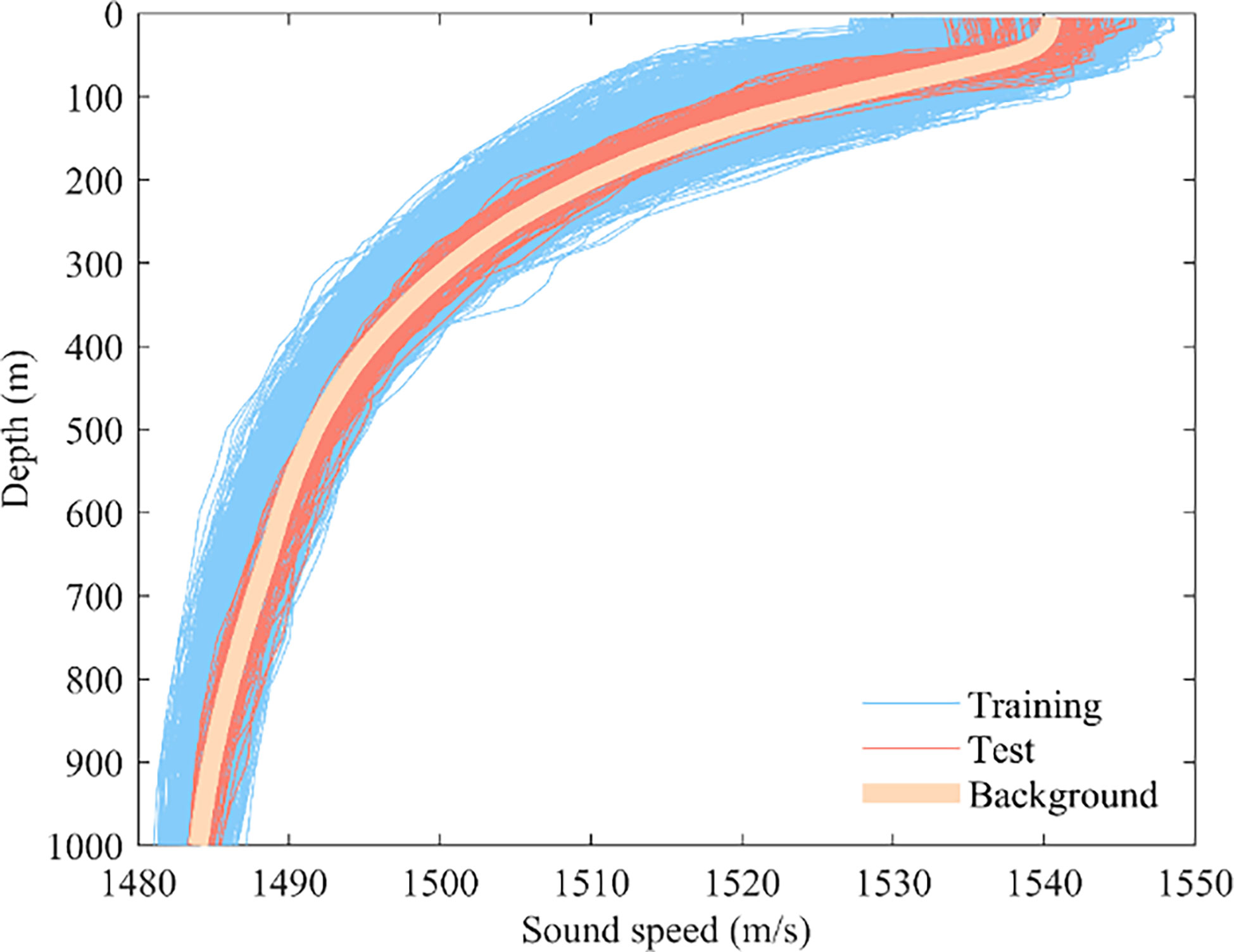
Figure 1 Sound speed profile samples and background profile.

3 Materials and methods

3.1 EOF dimensionality reduction

In solving problem of SSP inversion, the SSP are firstly reduced in dimensionality. The samples are usually reduced in dimensionality to represent the sound speed perturbation by the sound speed basis function. The sound speed can then be modeled using a function of time sampling point t and depth z in the form of:

$\begin{array}{ll}C(z,t)=C_0+{\displaystyle {\sum }_{i=1}^{\infty }}{a}_i(t)k_i(z)& (1)\end{array}$

where C₀ is the background profile, the part of the ocean where the sound speed is stable and constant over time, and can usually be approximated by the mean value. The part perturbed with time and depth is represented as a superposition of the EOF vector k_i(z) and its projection coefficients a_i(t). During SSP reconstruction, the EOF vectors of higher-order modes may contain too much noise. Therefore, the SSP perturbation can be effectively described using no more than a five orders EOF vector while ensuring little loss of SSP information. A five orders EOF vector are used for characterization in this paper. The EOF vector is obtained by extracting the principal components of the sound speed sample matrix, which is obtained by bringing the profile’s temperature, salinity, and depth data into the empirical equation for the sound speed (Del Grosso, 1974). The samples are subtracted from the climatic state sound speed profile values representing the background mean to the matrix form ω of the sound speed anomaly data.

$\begin{array}{ll}R=\omega \times {\omega }^T& (2)\end{array}$

$\begin{array}{ll}R\times E=E\times \Lambda & (3)\end{array}$

where R is the covariance matrix of the sound speed anomaly matrix, E is the EOF vector, and the first five orders vector is chosen as the inversion basis function.

Figure 2 shows the first five orders of the normalized vector of the EOF. Based on the amplitude distribution, it is known that the perturbation of the sound speed mainly occurs in the range of 0-200 m sea depth, and the amplitude has tended to zero at 1000 m. Thus this experimental study focuses on the reconstruction effect in the first 1000 m sea depth.

FIGURE 2

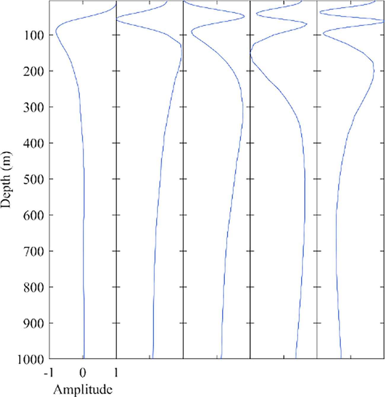
Figure 2 First five orders of the empirical orthogonal function.

3.2 Error analysis

The error analysis uses RMSE as the error assessment criterion for full text., where C_r is the measured profile and C is the reconstructed profile. Where m is the number of depth sampling points and n is the number of samples.

$\begin{array}{ll}RMSE=\sqrt{\frac{{\sum }_{i=1}^m{\sum }_{j=1}^n{(C_{r(i,j)}-C_{(i,j)})}^2}{m\times n}}& (4)\end{array}$

Table 1 shows the variance contribution of the first five orders of EOF modes, with the first five orders accounting for 96.1% of all eigenvalues. The direct reconstruction error of the first five orders is 1.03 m/s. This indicates that the first five orders EOF modes already contain the main features of the data, suggesting that they are sufficient for reconstructing the profiles and do not introduce too much perturbation noise from the higher-order modes.

TABLE 1

Table 1 Properties of reconstruction of different orders of the empirical orthogonal function.

3.3 Sample classification

During the experiment, author tested the accuracy performance of k at different values. It is found that the accuracy increases as the value of K increases. However, when K>3, the increase is very small, and the experimental cost and the accuracy gain are not proportional, so this paper uses K=3 to solve the difficulty of dividing the grid when the sample is insufficient. with the following procedure.

1. Determine the total number of classifications K = 3

2. K data vectors are randomly selected as the barycenter using the projection coefficients a_i as the training set.

3. Calculate the Euclidean distance of each projection vector to the K prime centers and classify the vector to the class with the smallest Euclidean distance.

4. After all vectors are classified, the center of mass of each cluster is recalculated.

5. The distance between the new center of mass and the original center of mass in step 4 is calculated, and when it is less than the set threshold, it is judged to be converged, and the classification is finished. If the threshold is not reached, steps 3 to 5 are repeated until convergence is achieved,

$\begin{array}{ll}{d}_i^m=\frac{1}{N_m}{\displaystyle {\sum }_{n=1}^N}{\delta }_{mn}{a}_i^n& (5)\end{array}$

The projection coefficient a_i is the training set, where n is the sample order, N is the total number of samples, and N_m denotes the total number of samples in the m cluster. $a_i^n$ denotes the i element of the n sample and is used to determine whether sample n belongs to cluster m. If it does, δ_mn=1, otherwise δ_mn=0. Based on $d_i^m$, the Euclidean distance ϵ can be calculated for all clusters,

$\begin{array}{ll}ϵ=\sqrt{{\displaystyle {\sum }_{n=1}^N}{\displaystyle {\sum }_k^K}{\delta }_{m_n}{\displaystyle {\sum }_{i=1}^S}{(a_i^n-d_i^m)}^2}& (6)\end{array}$

where S is the EOF number of orders used for inversion. A smaller ϵ indicates a smaller standard deviation for all clusters, indicating a better clustering effect.

3.4 Profile estimation based on remote sensing data

The SOM inversion process is briefly described as follows (Chapman and Charantonis, 2017; Li et al., 2021).

1. Initialization: the weight vectors are initialized along a linear subspace tensor of the two principal feature vectors of the input dataset in an ordered manner.

2. A sample vector x is randomly selected from the input training dataset, and the degree of similarity between it and all the weight vectors on the map is calculated, The best matching unit (BMU) denoted as y_c. The similarity is a metric using the Euclidean distance.

$\begin{array}{ll}\Vert \text{x}-{\text{y}}_{\text{c}}\Vert =mi{n}_i\left\{\Vert x-y_i\Vert \right\}& (7)\end{array}$

3. After finding the BMU, the prototype vector for the SOM was done using a batch algorithm by simply replacing the prototype vector with a weighted average of the samples, where the weighting factor is the neighborhood area function value,

$\begin{array}{ll}{y}_i(t+1)=\frac{{\sum }_{j=1}^n{h}_{ic(j)}(t)x_j}{{\sum }_{j=1}^n{h}_{ic(j)}(t)}& (8)\end{array}$

where c(j) is the BMU of the sample vector x_j, h_ic(j) is the neighborhood function (weighting factor), and n is the number of sample vectors.

4. Select another learning data input to the network’s input layer and return to step 2) until all the input data is provided to the network.

5. Let t = t + 1, return to step 2, and stop when training times T are reached.

After the neural network is trained, the inversion calculation is performed using known data. By using the existing data to find the nearest best matching unit in the neural network in terms of Euclidean distance, and using the best matching unit to complete the network parameters, where the parameters to be completed are the inversion coefficients.

$\begin{array}{ll}{d}_E^c(X,re{f}^c)={\sum }_{i\in avail}(1+{\sum }_{j\in minssing}{(co{r}_{ij}^c)}^2)\times {(X_i-re{f}_i^c)}^2& (9)\end{array}$

where X is the input data, cis the index of each type, ref is the reference vector, $d_E^c$ is the Euclidean distance between the input vector and the map cell, $co{r}_{ij}^c$ is the correlation between the known information and the information of the water body to be inverted, X_i is the known information, avail is the set of known information, and minssing is the set of unknown information. The SSP reconstruction is performed by obtaining the set of projection coefficients. The entire specific flow chart is as Figure 3 (Ou et al., 2022b).

FIGURE 3

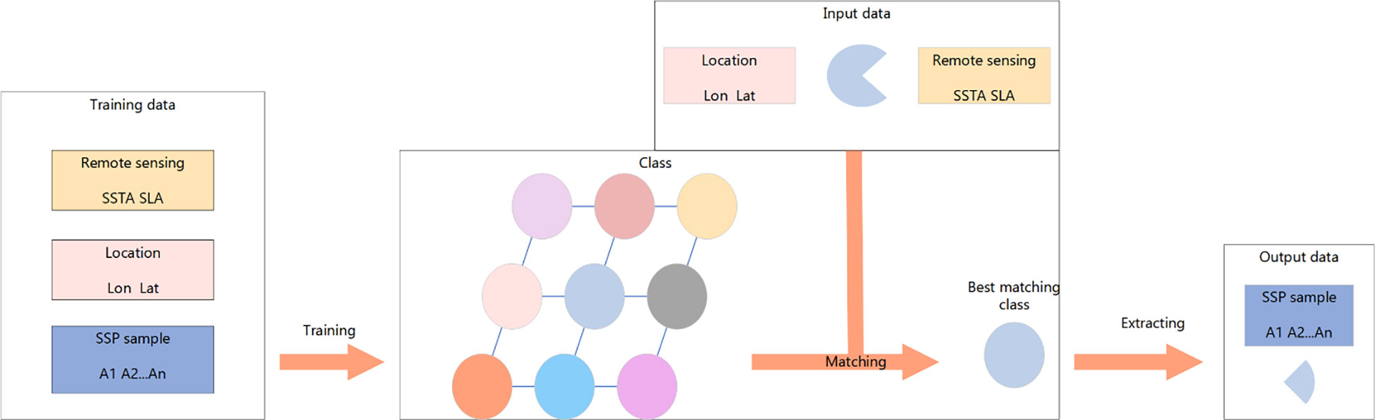
Figure 3 SOM algorithm inversion process.

4 Results and discussion

The experimental sea area was divided into three categories according to the EOF’s consistency. The sample numbers of Type 1, Type 2 and Type 3 are 1746, 612 and 1399 respectively, and the marker colors are Red, Pale yellow and Blue respectively.

Figure 4 shows the geospatial distribution of each type of training sample data, with the first type of samples concentrated in the inland river basin on the Xisha Islands side, the second type of samples concentrated in the coastal waters near the Philippines and Vietnam, and the third type of samples concentrated in the watershed on the Philippines side.

FIGURE 4

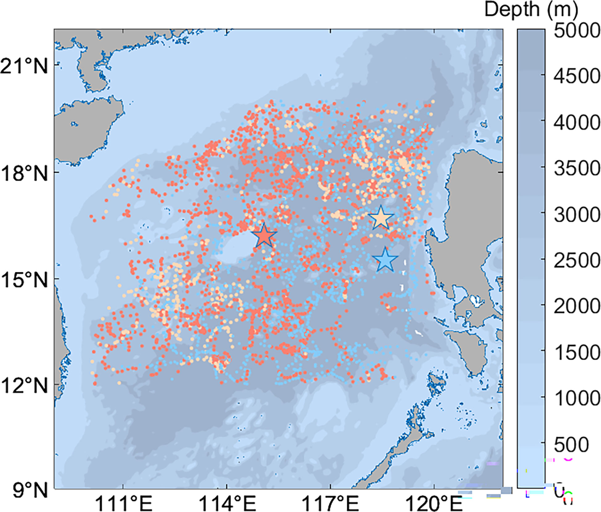
Figure 4 Distribution of samples after classification, asterisks mark class centers.

Figure 5 shows the seasonal time distribution of the number of training sample data in each category. The first sample data category is mainly distributed from December to May, with a small number of samples from June to September. The overall season of the first category of data is biased toward winter. The second sample data category is mainly distributed in October-April, with almost zero samples in summer, and the overall data season is winter. The third category of data sample data is primarily distributed from June to November, with an overall seasonal bias towards summer and autumn.

FIGURE 5

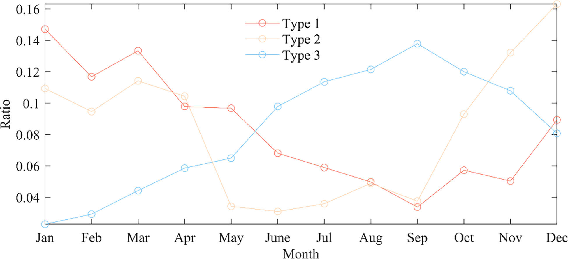
Figure 5 Seasonal distribution of sample data.

Figure 6 shows the errors for each sample in the test set. Except for very few samples, the errors after K-means classification and reconstruction using the SOM are all below 4.3 m/s, which is significantly more accurate than the traditional method of using the sea as a large grid with direct inversion using the SOM. The maximum reconstruction error for the K-means+SOM model in the test set samples was 4.29 m/s, and the maximum reconstruction error for the SOM model was 5.79 m/s.

FIGURE 6

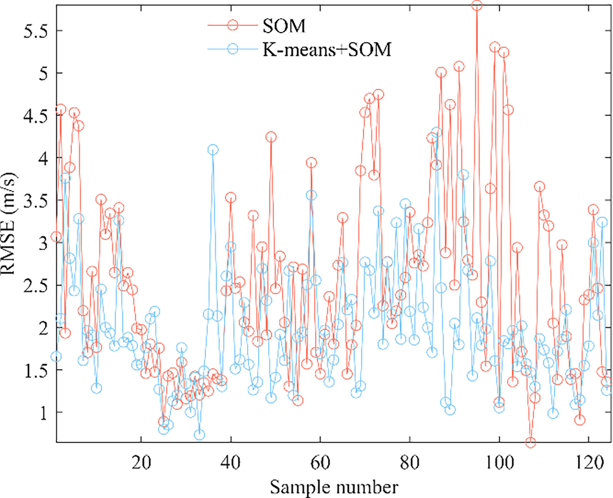
Figure 6 Error per sample for the test set.

Figure 7 shows the errors of the two reconstruction modes for each depth sampling point. From the modal plots and the sampling point error plots, it is known that the sound speed perturbations are most intense, and the amplitude is greatest at 100-200 m sea depth. As the temperature is the main factor affecting large variations in sound speed in the upper ocean, it is inferred that the error at this depth is due to seasonal and diurnal variations in the mixed layer to the extent that large variations in SSP are produced. Ocean internal waves and other dynamic ocean activity also contribute to some extent to the concentration of errors at these depths. The lower error at the sea surface is because near-surface SSP are directly controlled and estimated by sea surface parameters. And the errors will naturally be relatively small in deeper layers with less sound speed perturbance. The reconstruction accuracy of the K-means+SOM model is significantly higher than that of the SOM model, except for very few depth sampling points. The maximum reconstruction error of the K-means+SOM model is 3.08 m/s at the sound speed perturbation. In comparison, the maximum reconstruction error of the SOM model is 5.22 m/s at the sound speed perturbation, indicating that the classified and then inverse model characterizes the sound speed perturbation to a greater extent. The error analysis of the sample sequence and the depth reconstruction data show that this classification model followed by inversion has high accuracy. The vast majority of the improvement in accuracy of the post-class inversion is because classification refines the EOF vectors of the samples, which in the traditional method using a large grid are of one class, to three classes after classification refinement. The EOF vectors of samples with the same and similar characteristics are naturally the same and similar. EOF vector analysis was performed on the classified samples of the three categories, correspondence analysis of the time and space distribution, and time and space functions of the three types of samples to verify this conclusion.

FIGURE 7

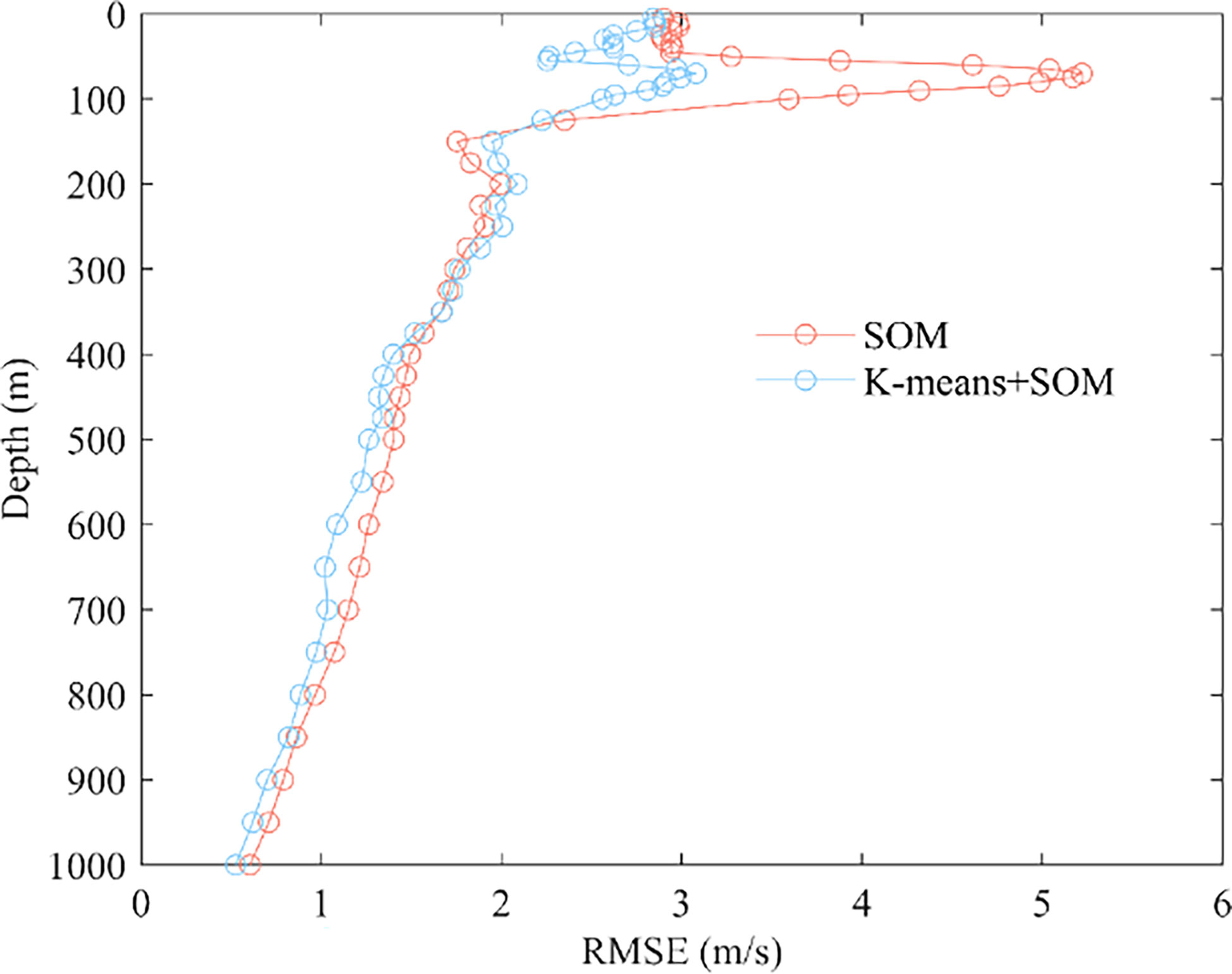
Figure 7 Error per depth of the test set.

The first-order mode contribution of Type 1 is 63.9%, and the second-order mode contribution is 20.6%. The features are mainly concentrated in the first mode, and the second-order mode accounts for a certain proportion of the features. The sound speed perturbations of the first two modes are concentrated in the ocean’s upper layer above 200 m sea depth. The modal contribution of the first five orders is 96.3%, which already covers most features. The direct reconstruction error of the first five orders is 0.86 m/s, which is sufficiently accurate to use the first five orders for characterization and does not introduce too much perturbation noise from the higher order modes (Table 2).

TABLE 2

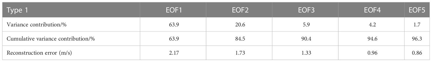
Table 2 First five orders contribution rates and errors for Type 1.

The first-order mode contribution of Type 2 is 93.3%, and the features are mainly concentrated in the first mode. The sound speed disturbances in the first-order mode are all concentrated in the ocean’s surface layer above 100 m sea depth. The first five order modal contribution is 99.0%, which covered the sample features. The direct reconstruction error of the first five orders modal is 1.82 m/s; using the first five orders modal representation has covered the original features of the sample (Table 3).

TABLE 3

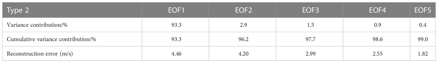
Table 3 First five orders contribution rates and errors for Type 2.

The first-order mode contribution of Type 3 is 72.2%. The second-order mode contribution is 14.4%, with the features mainly concentrated in the first mode and the second-order mode accounting for a certain proportion of the features. The sound speed perturbance in the first two modes are concentrated in the ocean’s upper layer above 200 m sea depth. The modal contribution of the first five orders is 96.2%, which already contains the majority of the sample features. The use of the first five orders of modal representation has largely encompassed the majority of the sample features. This sample data category is influenced by factors such as black tides, monsoons, and wider geographical distribution. It is the most challenging part of the three categories of sample data to characterize. The consistency of the EOF vectors is low relative to the first two categories, with a direct reconstruction error of 4.80 m/s for the first five orders of modalities (Table 4).

TABLE 4

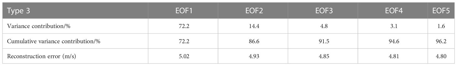
Table 4 First five orders contribution rates and errors for Type 3.

According to the law that the EOF first-order mode contribution is the majority, the EOF first-order mode can already be roughly analyzed to derive the sound speed variation law (Figure 8). Therefore, the first order mode of the EOF analysis of the three types of samples can be used as a function of space, and the average of the projection coefficients can be used as a function of time to analyze the change in sound speed for each type of data.

FIGURE 8

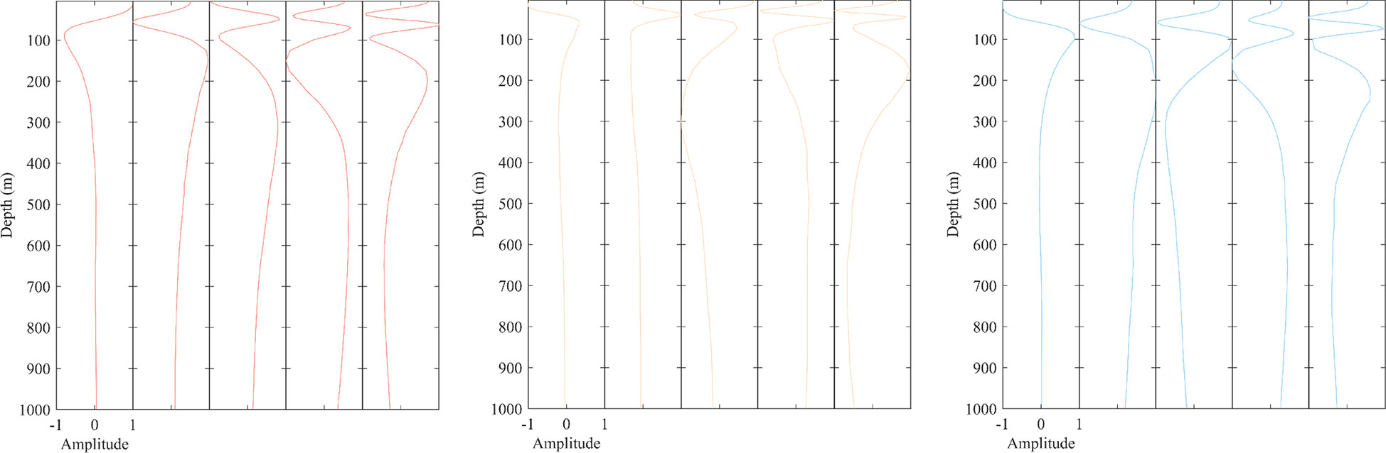
Figure 8 The first five orders of modalities of Type 1~Type3.

Figure 9 shows the trend of sound speed variation as a function of time and space for the first type of data, the perturbation of the sound speed reaches its maximum near 100 m depth, with the overall sound speed variation being large at the surface and small at the deep-seated. The perturbance gradually decreases with increasing depth, reaching around 400 m, where it tends to zero, and after that, it does not change much with increasing depth. As a function of time, the mean amplitude of sound speed has negative values, with the maximum value in the summer months when the data sample is small, in line with the seasonal transformation of the first type of sample data. Combined with the spatial and temporal distribution, the first data type is spatially distributed on the western side of the South China Sea, and the temporal distribution is skewed towards winter. Influenced by the monsoon in the northeastern part of the South China Sea in winter, the frequent intrusion of cold air can cause significant cooling of the seawater in this region resulting in a negative trend in the temporal and spatial amplitude of the sound speed variation.

FIGURE 9

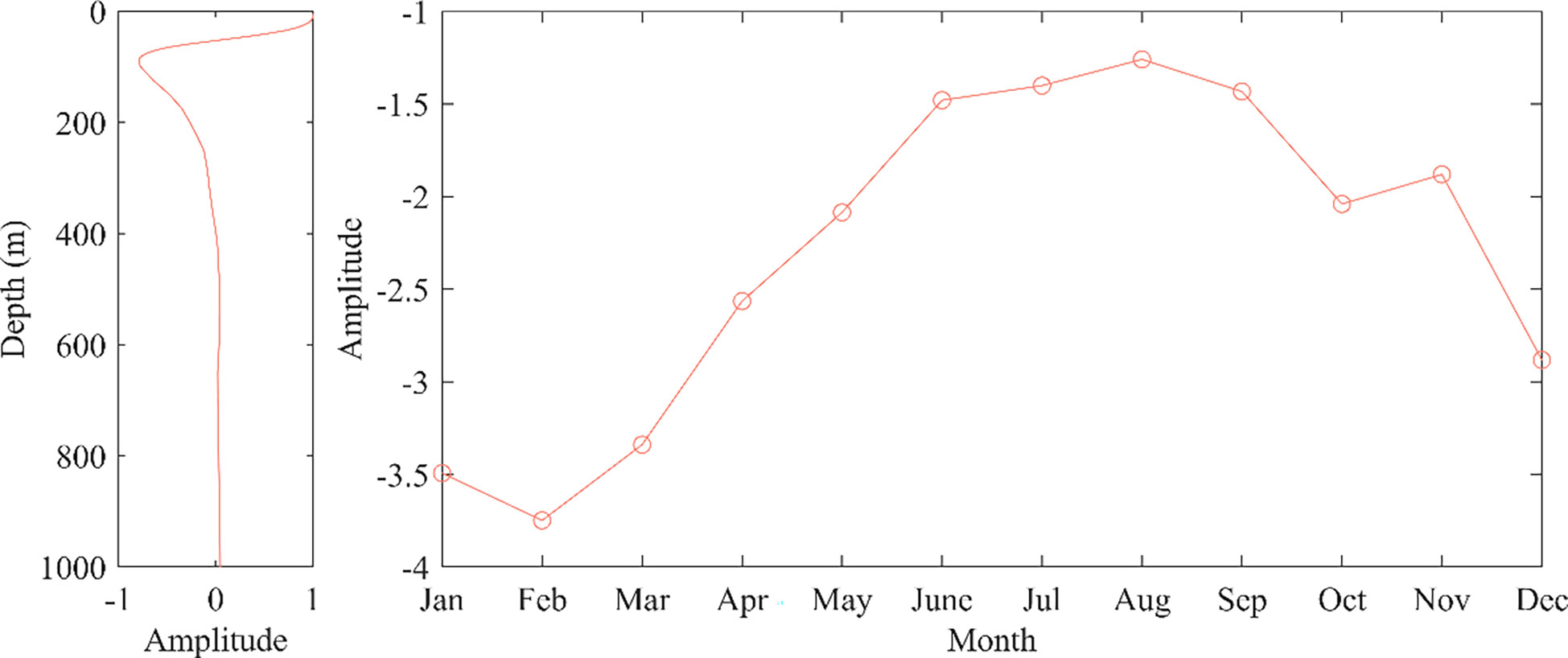
Figure 9 Time and space functions of Type 1.

Figure 10 shows the trend of sound speed variation as a function of time and space for the second type of data, from the perspective of the spatial function, similar to the first type of data, the perturbation of sound speed reaches a maximum near 100 m depth, with the overall sound speed variation being large at the surface and small at the deep-seated. The perturbance gradually decreases with increasing depth, reaching around 400 m and tending to zero, with little change with increasing depth after that. As a function of time, the amplitude values of the sound speed are all negative, which corresponds to the seasonal transformation of the second type of sample data. Combined with the spatial and temporal distribution, the second type of data is spatially distributed in the northern part of the South China Sea and the cold water area near the coast of Vietnam, with a temporal distribution biased towards winter. The northern part of the South China Sea is influenced by the winter monsoon in the northeastern part of the South China Sea, and the frequent intrusion of cold air can cause significant cooling of the seawater in this region resulting in a negative trend in the temporal and spatial amplitude of the sound speed variation. The waters close to the coast of Vietnam can form cold upwelling waters due to the cold summer eddies in the western South China Sea, creating a cold water zone. The effects of the monsoon and upflow cause the samples in this category to show negative values in sound speed variation perturbation and time and space functions.

FIGURE 10

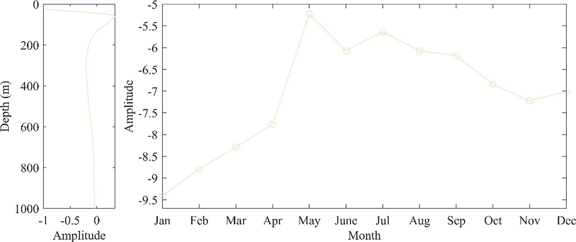
Figure 10 Time and space functions of Type 2.

Figure 11 shows the trend of sound speed variation as a function of time and space for the third type of data, from the perspective of the spatial function, similar to the first two types of data, the perturbation of sound speed reaches a maximum near 100 m depth, with a large variation in overall sound speed variation at the surface and a small variation at the deep-seated. The perturbance gradually decreases with increasing depth, reaching around 400 m, where it tends to zero, and after that, it does not change much with increasing depth. As a function of time, the amplitude of sound speed has a positive value, which corresponds to the seasonal transformation of the type 3 sample data. Combined with the spatial and temporal distribution, the third type of data is spatially distributed on the eastern side of the South China Sea, with distribution in both the north and south. The temporal distribution is skewed towards summer. The influence of the southwest monsoon in summer and the heat and salt transported to the northern part of the South China Sea from the eastern side of the Bus Strait to the northern part of the South China Sea by the Kuroshio tide will warm up the seawater. Sound speed variation’s time and space functions for this type of sample show positive values in magnitude.

FIGURE 11

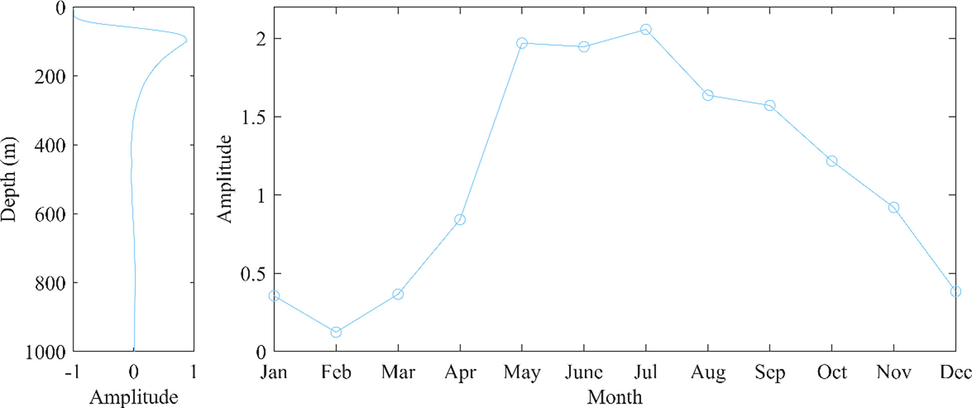
Figure 11 Time and space functions of Type 3.

The K-means algorithm divides the South China Sea waters into three categories of training data samples based on the consistency of EOF. The correspondence analysis results between the time and space distribution and the time and space functions show that this classification has some justification for classifying samples that are similar in time and space into similar categories. Based on the results of the analysis of reconstruction errors and time and space functions. The K-means-based pre-classification scheme effectively solves the difficulty of dividing the training grid for machine learning algorithms in complex, under-sampled seas and also enables de-gridded SSP inversion for complex, under-sampled seas. This is reflected in the refinement of the EOF vector in the classification and the rational division of samples with the same geographical location and similar hydrological characteristics in terms of geographical distribution and time season. The time-seasonal distribution of the sample data corresponds well to the time function.

5 Conclusions

Sound speed profiles are one of the elements of marine environmental observations, and real-time, accurate sound speed profile information is important for various marine acoustic studies. Previous scholars have proved that projecting the sea surface data acquired by satellite remote sensing technology into the ocean and performing SSP inversion to obtain large-scale sound speed data is feasible and effective. However, due to the non-linear and distinctive characteristics of the ocean, the accuracy of the inversion using the traditional linear inversion method through physical relationships is low and not applicable in a complex class of sea in the South China Sea when there are complex climatic, seasonal variations and geographical environments in certain sea areas. The accuracy of inversion using machine learning methods is undoubtedly improved. Still, it is also limited by the fact that gridded inversion requires a certain number of samples in each grid. This is also not applicable in sea areas where the spatial and temporal distribution of sample data is sparse due to various reasons such as political reasons, observation environment, and harsh natural environment. Therefore, this paper proposes an EOF-based grid-free pre-classification scheme. It abandons the idea that machine learning algorithms consistently divide the sea area into 1°×1° or 2°×2° latitude and longitude grid cells or treat the whole sea area as a large grid for inversion, and divides the training classes according to the consistency of EOF, refining the EOF vector.

In this paper’s classification of the South China Sea area, the scheme divides the sea area into three types of data samples with similarity in spatial and temporal distribution. Each type of sample corresponds better to the South China Sea area in terms of time and geographical environmental factors, such as the southwest monsoon in summer, the northeast monsoon in winter, the northern Kuroshio, and the cold water upwelling formed by the western summer cold eddies. The results of the experimental error analysis also show that the classification followed by the inversion scheme consistently improves the model’s accuracy by more than 20% compared to direct inversion using machine learning algorithms. The accuracy of the inversion results is also improved in the most difficult to characterize major sound speed perturbance at depths of 100-200 m.

In future research, we can try to introduce more geographic, physical, and climate-based multi-source constraints to refine the classification conditions to obtain better classification results. For example, setting the monsoon constraint parameter to classify the sea areas affected by monsoon that cause temperature increase or decrease into one category. According to the geographical location, the sea areas affected by the flow field are classified into the same category. Samples with similar depth range of sound speed perturbance are classified into one category according to the different main sound speed perturbance in the sea area. The introduction of more constraints for classification should be able to bring the accuracy of SSP inversion further, under the premise of ensuring interpretability in physical sense.

Data availability statement

The original contributions presented in the study are included in the article/supplementary material. Further inquiries can be directed to the corresponding author.

Author contributions

CL completed the literature research, analysis, and manuscript writing. KQ completed the conceptualization, methodology and funding acquisition. All authors contributed to the article and approved the submitted version.

Funding

This research was funded by the Natural Science Foundation of Guangdong Province, grant number No.2022A1515011519 and funded by the Innovation Training Funding Project for College Students, grant number No.S202210566001.

Conflict of interest

The authors declare that the research was conducted in the absence of any commercial or financial relationships that could be construed as a potential conflict of interest.

Publisher’s note

All claims expressed in this article are solely those of the authors and do not necessarily represent those of their affiliated organizations, or those of the publisher, the editors and the reviewers. Any product that may be evaluated in this article, or claim that may be made by its manufacturer, is not guaranteed or endorsed by the publisher.

References

Bao S., Zhang R., Wang H., Yan H., Yu Y., Chen J. (2019). Salinity profile estimation in the pacific ocean from satellite surface salinity observations. J. Atmospheric Oceanic Technol. 36 (1), 53–68. doi: 10.1175/JTECH-D-17-0226.1

CrossRef Full Text | Google Scholar

Bianco M., Gerstoft P. (2017). Dictionary learning of sound speed profiles. J. Acoustical Soc. America 141 (3), 1749–1758. doi: 10.1121/1.4977926

CrossRef Full Text | Google Scholar

Carnes M. R., Teague W. J., Mitchell J. L. (1994). Inference of subsurface thermohaline structure from fields measurable by satellite. J. Atmospheric Oceanic Technol. 11 (2), 551–566. doi: 10.1175/1520-0426(1994)011<0551:IOSTSF>2.0.CO;2

CrossRef Full Text | Google Scholar

Chapman C., Charantonis A. A. (2017). Reconstruction of subsurface velocities from satellite observations using iterative self-organizing maps. IEEE Geosci. Remote Sens. Lett. 14 (5), 617–620. doi: 10.1109/LGRS.2017.2665603

CrossRef Full Text | Google Scholar

Charantonis A. A., Badran F., Thiria S. (2015). Retrieving the evolution of vertical profiles of chlorophyll-a from satellite observations using hidden Markov models and self-organizing topological maps. Remote Sens. Environ. 163, 229–239. doi: 10.1016/j.rse.2015.03.019

CrossRef Full Text | Google Scholar

Chen C., Ma Y., Liu Y. (2018). Reconstructing sound speed profiles worldwide with Sea surface data. Appl. Ocean Res. 77, 26–33. doi: 10.1016/j.apor.2018.05.002

CrossRef Full Text | Google Scholar

Chen C., Yan F., Gao Y., Jin T., Zhou Z. (2020). Improving reconstruction of sound speed profiles using a self-organizing map method with multi-source observations. Remote Sens. Lett. 11 (6), 572–580. doi: 10.1080/2150704X.2020.1742940

CrossRef Full Text | Google Scholar

Chu P. C., Guihua W., Fan C. (2004). Evaluation of the US navy’s modular ocean data assimilation system (MODAS) using south china sea monsoon experiment (SCSMEX) data. J. Oceanogr. 60 (6), 1007–1021. doi: 10.1007/s10872-005-0009-3

CrossRef Full Text | Google Scholar

Del Grosso V. A. (1974). New equation for the speed of sound in natural waters (with comparisons to other equations). J. Acoustical Soc. America 56 (4), 1084–1091. doi: 10.1121/1.1903388

CrossRef Full Text | Google Scholar

Fischer M. (2000). Multivariate projection of ocean surface data onto subsurface sections. Geophys. Res. Lett. 27 (6), 755–757. doi: 10.1029/1999GL010451

CrossRef Full Text | Google Scholar

Frederick C., Villar S., Michalopoulou Z. H. (2020). Seabed classification using physics-based modeling and machine learning. J. Acoustical Soc. America 148 (2), 859–872. doi: 10.1121/10.0001728

CrossRef Full Text | Google Scholar

Han N., Yao S. (2021). Discrimination of the active submerged/bottom target based on the total scintillation index. Appl. Acoustics 172, 107646. doi: 10.1016/j.apacoust.2020.107646

CrossRef Full Text | Google Scholar

Hjelmervik K. T., Hjelmervik K. (2013). Estimating temperature and salinity profiles using empirical orthogonal functions and clustering on historical measurements. Ocean Dynamics 63 (7), 809–821. doi: 10.1007/s10236-013-0623-3

CrossRef Full Text | Google Scholar

Jain S., Ali M. M. (2006). Estimation of sound speed profiles using artificial neural networks. IEEE Geosci. Remote Sens. Lett. 3 (4), 467–470. doi: 10.1109/LGRS.2006.876221

CrossRef Full Text | Google Scholar

LeBlond P. H. (1976). Temperature–salinity analysis of world ocean waters. J. Fish. Res Board of Canada 33 (6), 1471–1471. doi: 10.1139/f76-190

CrossRef Full Text | Google Scholar

Li Y., Gao P., Tang B., Yi Y., Zhang J. (2022a). Double feature extraction method of ship-radiated noise signal based on slope entropy and permutation entropy. Entropy 24, 22. doi: 10.3390/e24010022

CrossRef Full Text | Google Scholar

Li Y., Geng B., Jiao S. (2022b). Dispersion entropy-based lempel-ziv complexity: A new metric for signal analysis. Chaos Solitons Fractals 161, 112400. doi: 10.1016/j.chaos.2022.112400

CrossRef Full Text | Google Scholar

Li Y., Jiao S., Geng B. (2022c). Refined composite multiscale fluctuation-based dispersion lempel–ziv complexity for signal analysis. ISA Trans. doi: 10.1016/j.isatra.2022.06.040

CrossRef Full Text | Google Scholar

Li H., Qu K., Zhou J. (2021). Reconstructing sound speed profile from remote sensing data: Nonlinear inversion based on self-organizing map. IEEE Access 9, 109754–109762. doi: 10.1109/ACCESS.2021.3102608

CrossRef Full Text | Google Scholar

Li Y., Tang B., Yi Y. (2022d). A novel complexity-based mode feature representation for feature extraction of ship-radiated noise using VMD and slope entropy. Appl. Acoustics 196, 108899. doi: 10.1016/j.apacoust.2022.108899

CrossRef Full Text | Google Scholar

Liu Y., Weisberg R. H. (2005). Patterns of ocean current variability on the West Florida shelf using the self-organizing map. J. Geophys. Res. 110, C06003. doi: 10.1029/2004JC002786

CrossRef Full Text | Google Scholar

Meijers A. J. S., Bindoff N. L., Rintoul S. R. (2011). Estimating the four-dimensional structure of the southern ocean using satellite altimetry. J. Atmospheric Oceanic Technol. 28 (4), 548–568. doi: 10.1175/2010JTECHO790.1

CrossRef Full Text | Google Scholar

Nardelli B. B., Santoleri R. (2004). Reconstructing synthetic profiles from surface data. J. Atmospheric Oceanic Technol. 21 (4), 693–703. doi: 10.1175/1520-0426(2004)021<0693:RSPFSD>2.0.CO;2

CrossRef Full Text | Google Scholar

Ou Z., Qu K., Liu C. (2022a). Estimation of sound speed profiles using a random forest model with satellite surface observations. Shock Vibration 2022, 2653791. doi: 10.1155/2022/2653791

CrossRef Full Text | Google Scholar

Ou Z., Qu K., Wang Y., Zhou J. (2022b). Estimating sound speed profile by combining satellite data with In situ Sea surface observations. Electronics 11 (20), 3271. doi: 10.3390/electronics11203271

CrossRef Full Text | Google Scholar

Rouseff D., Jackson D. R., Fox W. L. J., Jones C. D., Ritcey J. A., Dowling D. R. (2001). Underwater acoustic communication by passive-phase conjugation: Theory and experimental results. IEEE J. Oceanic Eng. 26 (4), 821–831. doi: 10.1109/48.972122

CrossRef Full Text | Google Scholar

Song A. (2017). High frequency underwater acoustic communication channel characteristics in the gulf of Mexico. J. Acoustical Soc. America 141 (5), 3990–3990. doi: 10.1121/1.4989133

CrossRef Full Text | Google Scholar

Stojanovic M., Catipovic J. A., Proakis J. G. (1994). Phase-coherent digital communications for underwater acoustic channels. IEEE J. Oceanic Eng. 19 (1), 100–111. doi: 10.1109/48.289455

CrossRef Full Text | Google Scholar

Su H., Yang X., Lu W., Yang W. H. (2019). Estimating subsurface thermohaline structure of the global ocean using surface remote sensing observations. Remote Sens. 11 (13), 1598. doi: 10.3390/rs11131598

CrossRef Full Text | Google Scholar

Sun S., Fang Y., Zu Y., Liu B., Samah A. A. (2020). Seasonal characteristics of mesoscale coupling between the sea surface temperature and wind speed in the south China Sea. J. Climate 33 (2), 625–638. doi: 10.1175/JCLI-D-19-0392.1

CrossRef Full Text | Google Scholar