Main drivers of marine heat waves in the eastern South Pacific

During the last decades, marine heat waves (MHWs) have increased in frequency and duration, with important impacts on marine ecosystems. This trend has been related to rising global sea surface temperatures, which are expected to continue in the future. Here, we analyze the main characteristics and possible drivers of MHWs in the eastern South Pacific off Chile. Our results show that MHWs usually exhibit spatial extensions on the order of 10³-10⁴ km², temperature anomalies in the mixing layer between 1 and 1.3°C, and durations of 10 to 40 days, with exceptional events lasting several months. In this region, MHW are closely related to the ENSO cycles, in such a way that El Niño and, to a lesser extent, La Niña events increase the probability of high intensity and extreme duration MHWs. To analyze the MHW drivers, we use the global ocean reanalysis GLORYS2 to perform a heat budget in the surface mixed layer. We find that most events are dominated by diminished heat loss –associated with reduced evaporation– and enhanced insolation; thus, this group is called ASHF (for air-sea heat fluxes). The second type of MHWs is driven by heat advection, predominantly forced by anomalous eastward surface currents superimposed on a mean westward temperature gradient. The third type of MHWs results from a combination of positive (seaward) anomalies of air-sea heat fluxes and heat advection; this group exhibits the greatest values of spatial extension, intensity, and duration.

1 Introduction

Marine heat waves (MHWs), defined as extreme positive anomalies in sea surface temperature (SST), have trended upwards in frequency as well as temporal and spatial extents during the last few decades (Frölicher et al., 2018; Oliver, 2019; Marin et al., 2021). MHWs can have negative ecological and socioeconomic impacts (e.g., Hobday et al., 2018; Intergovernmental Panel on Climate Change (IPCC), 2022); in particular, they have been associated with a considerable decrease in primary production and a reduction in the biomass of certain marine species (Smale and Wernberg, 2013; Cavole et al., 2016; Reed et al., 2016; Arafeh-Dalmau et al., 2020; Sen Gupta et al., 2020). MHWs may also impact the spatial distribution of some species, altering the typical spatial ranges some organisms occupy (e.g., Bond et al., 2015; Smale et al., 2019; Jacox et al., 2020). Whereas the habitats of some species have been observed to shrink spatially, those of tropical species tend to extend (e.g., Wernberg et al., 2013; Cavole et al., 2016). Furthermore, harmful algal blooms have also been related to MHWs (e.g., McCabe et al., 2016). Most of the impacts induced by MHWs have impacted the fishing industry, greatly reducing catches and even completely disabling the fishing of certain species due to harmful algal blooms (Caputi et al., 2016; McCabe et al., 2016). MHWs are also an important issue for the regulation of marine resources since they could impose stressful environmental conditions on species that have already seen their traditional habitat reduced by other factors (Frölicher and Laufkötter, 2018). Thus, a better understanding of the MHW drivers and occurrences would improve their predictability on different time scales and support decision makers in mitigating their negative impacts.

Many processes on different spatial and temporal scales are involved in the generation of MHWs (Holbrook et al., 2019). Even the ongoing global warming has been directly related to a higher probability of extreme MHWs (Oliver et al., 2019). Given the current global warming scenario and according to global projections for the end of the present century, the number of MHWs across the entire ocean is projected to increase 10-fold (Frölicher et al., 2018). Over central Chile (26°S-39°S), a slightly positive warming trend that increases south of ~38°S has been observed between 1982 and 2020. This trend has been associated with an increasing frequency of MHWs (Varela et al., 2021; Pujol et al., 2022). The warming trend off Chile will continue and probably increase in the future, being more severe along the length of the Chilean coast (e.g., Dewitte et al., 2021). Nevertheless, observational evidence showed a cooling in the coastal region from 1979 to 2006, contrasting with the warming air temperature observed over continental Chile (Falvey & Garreaud, 2009).

Modes of internal climate variability can also impact the likelihood of MHWs and can maintain or intensify these events for long periods (Holbrook et al., 2019; Sen Gupta et al., 2020). In the Pacific Ocean, the positive phase of the Pacific Decadal Oscillation (PDO) leads to predominantly warm years, when MHWs tend to occur (Newman et al., 2016; Scannell et al., 2016). The warm phase of the PDO is also associated with positive feedback with El Niño events, contributing to the generation of large MHWs (more intense and with greater spatial and temporal extensions). Such is the case of the 2014-2016 event, which was categorized as severe, that occurred over much of the Northeast Pacific (Di Lorenzo and Mantua, 2016). El Niño events increase the probability of high-intensity MHWs in the eastern tropical Pacific (the intensity of a MHW refers to the temperature anomaly associated with the MHW, see methods below). In general, the greater the intensity of El Niño, the greater the intensity of the observed MHW. In terms of duration, MHWs related to El Niño events can last as long as the El Niño itself (Oliver et al., 2018; Sen Gupta et al., 2020). La Niña events may also force MHWs in the western Pacific. During the austral summer of 2010-2011, a MHW was induced by greater warm water advection off Western Australia, triggered in turn by an intensification of the Leeuwin Current due to the strong La Niña event (Pearce and Feng, 2013).

On timescales ranging from several days to several weeks, the MHW drivers generally act on regional-length scales, i.e., spanning from tens to hundreds of km (Holbrook et al., 2019). The frequency of MHWs lasting less than 100 days has increased in the last two decades along the coasts of Peru and northern Chile (Pietri et al., 2021). On this regional scale, the warming generated by heat advection (HA) is due to the action of anomalous currents through typical (mean) temperature gradients or typical currents flowing in anomalously large temperature gradients. For instance, the MHW observed in the Tasman Sea in 2015-2016 was generated by anomalies of the East Australian Current (Oliver et al., 2017). On the same spatial scale, the warming generated by air-sea heat fluxes (ASHFs) is also important. These conditions generally occur in the presence of atmospheric blocking, which reduces cloud cover, enhances solar radiation, and decreases surface wind speed, thereby reducing latent heat cooling (Holbrook et al., 2020). In turn, this causes a decrease in the mixed-layer depth (MLD) contributing further to the warming of this reduced water volume (Oliver et al., 2021). For instance, the MHW that occurred in the boreal winter of 2013-2014 over the northeast Pacific –with an intensity of ~2°C– was an event that began because of a weakening of the westerly surface winds and a large decrease in the MLD, which primarily decreased sensible and latent heat loss from the ocean to the atmosphere; moreover, this was coupled with a weakening of the cooling typically caused by advective flows in the area (Bond et al., 2015). Another mechanism of similar spatial and temporal scales is warming due to entrainment anomalies. This mechanism considers both the vertical advection of heat and the intrusion of heat towards more superficial layers due to the variation of the mixing layer (see equation 1 below). This process generally makes a minor contribution to the generation of MHWs (e.g., Holbrook et al., 2019). However, in coastal upwelling regions –like central Chile–, it is reasonable to assume that the weakening of this cooling process may increase the probability that MHWs will occur (Varela et al., 2021).

In this study, we evaluate the relative importance of the main drivers of MHW (ASHF, HA, and entrainment) in the southeastern Pacific for the last two decades (1992-2020). We perform a heat budget analysis of the MHWs observed in the surface mixed layer and, using different statistical criteria, evaluate the relative importance of these drivers in the generation of MHWs. A long, intense (anomalies greater than 3°C) MHW occurred in the tropical and subtropical Southeast Pacific during the austral summer of 2016-2017 associated with the “coastal El Niño” (Takahashi et al., 2018; Pujol et al., 2022). This event took place after the large central El Niño of 2015-2016 (also known as “Godzilla” El Niño). The dynamics of the coastal El Niño differed from those of the El Niño-Southern Oscillation. In fact, neutral temperature anomalies were observed in the equatorial Pacific during the coastal El Niño (Echevin et al., 2018; Takahashi et al., 2018). The large MHW related to this coastal El Niño event notoriously impacted our study region off central Chile. The present study analyzes this MHW in detail, along with the MHW induced by the prominent 1997-1998 El Niño event (McPhaden, 1999; McPhaden and Yu, 1999).

2 Materials and methods

2.1 Data

We use temperature, currents, and MLD from the GLORYS2-V4 Global Ocean Ensemble Physics Reanalysis (hereafter GLORYS; https://data.marine.copernicus.eu/product/GLOBAL_REANALYSIS_PHY_001_031/description) (Garric and Parent, 2017) for the period January 1993 to August 2019. This reanalysis is based on the NEMO ocean general circulation model version 3.1 (https://www.nemo-ocean.eu/). The ocean model assimilates satellite SST from AVHRR and AMSR-E (1/4° resolution), along-track sea-level anomalies derived from satellite altimetry, and temperature and salinity profiles from ARGO floats since 2002. The ocean model has a horizontal resolution of 1/4° curvilinear orthogonal grid and 75 vertical levels. NEMO’s surface boundary conditions are taken from ERA-Interim global atmospheric reanalysis (https://www.ecmwf.int/en/forecasts/datasets/reanalysis-datasets/era-interim) and includes zonal and meridional surface wind, latent and sensible heat fluxes, and net shortwave and longwave radiation. The ERA-Interim database, also used in the present study, has a temporal and spatial resolution of 6 h and approximately 80 km (3/4°), respectively, and 60 vertical levels from the surface to 0.1 hPa (Berrisford et al., 2011; Dee et al., 2011). Only sea surface data over the period from 1993 to August 2019 were used in this study. To achieve the same horizontal resolution as GLORYS (i.e., 1/4°), the ERA variables were interpolated using an Akima spline.

2.2 Definition of marine heat waves

MHWs were defined using the mixed layer mean temperature (MLT) following the methodology proposed by Hobday et al. (2016). When the daily MLT in a specific grid point exceeds a climatological threshold value for a period of at least 5 days, it is considered to be impacted by a MHW. Daily threshold values correspond to the 90th percentile of the MLT for each grid point. For the calculation of the 90th percentile for a specific day of the year, we used an 11-day moving window centered on the specific day and the 26-year-long time series (see Figure S1 in Supporting Information). Finally, the threshold values were smoothed using a 31-day moving mean (Hobday et al., 2016).

2.3 Characterization of MHWs

To characterize the MHW events, different metrics were used: duration, spatial extent, and mean and maximum intensities (Hobday et al., 2016). We also quantified the frequency of MHWs inside the study region based on the number of events per year.

2.3.1 Duration

The duration of a MHW is the number of days that the MLT continuously exceeds the threshold value (only if this number is greater than 5 days according to the MHW definition). To calculate duration, we considered our study region to be a unit (shown in Figure 1 as the area enclosed by the black contour). For this, we used two different definitions: one based on the MLT of each grid point and the other based on the complete study region. In the first case, the duration is the number of days during which the MHW is present in a particular grid point (named definition 1, used in Figure 1B). In the second case, the duration is the number of days during which at least one grid point within the study region was under the influence of a MHW; in this case, duration considers all grid points affected by a MHW within the study region at the same time (named definition 2, used in Figure 2). Both definitions are used here in different contexts and explicitly specified.

FIGURE 1

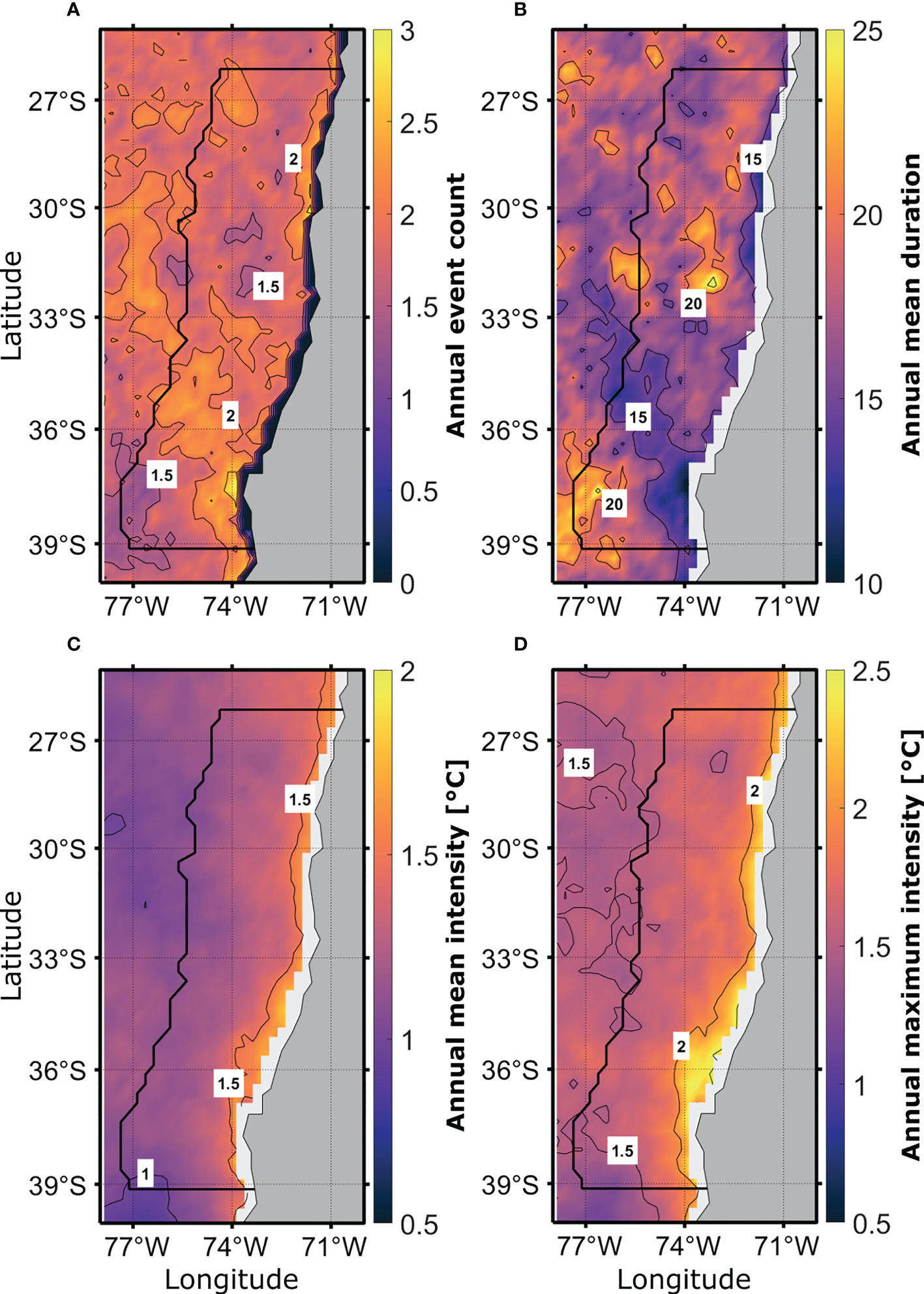
Figure 1 Annual mean of the different metrics that characterize the MHWs off central Chile: (A) mean frequency, (B) mean duration, (C) mean intensity, and (D) maximum intensity. The study region is enclosed by the black contour. Annual means were calculated between 1993 and 2018.

FIGURE 2

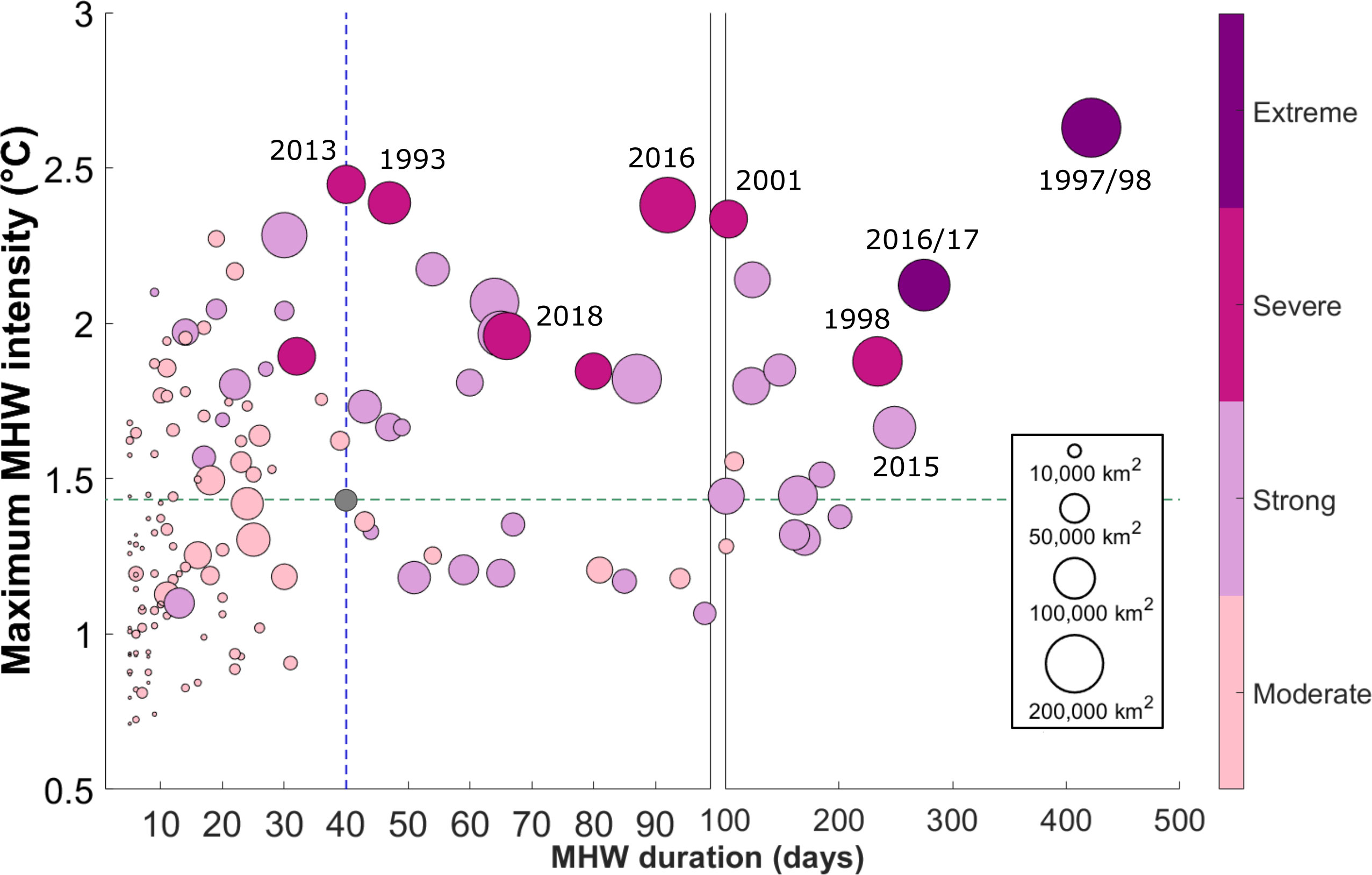
Figure 2 Maximum intensity versus duration of the MHWs off central Chile. Each event is represented by a circle. The size of each circle represents the spatial extent of the corresponding event according to the scale shown in the lower right corner. Colors show the event category according to the scale on the right side of the graph (see methodology –section 2.3– for more details).

2.3.2 Spatial extent

The spatial extent is the sum of the areas of all the grid points that satisfy the definition of a MHW during a given day.

2.3.3 Intensities

The mean MHW intensity is directly defined as the mean value of the mixed layer temperature anomalies at all grid points affected by the MHW (e.g., Oliver et al., 2021). The maximum intensity is calculated as follows: Firstly, for each day, the maximum MLT anomaly within the MHW impacted region is selected, and then all the maximum daily values are averaged over the period that the MHW lasted.

The historical ranges of different metrics are also shown to provide typical characteristics of the MHWs observed in our study region. These ranges are delimited by the 25th and 75th percentiles of the respective metrics.

Following Hobday et al. (2018), different categories of MHWs are used based on the difference between the climatological (mean) MLT and the threshold value defined above. Then, depending on the frequency with which the MLT exceeds this difference, different categories were defined: moderate, strong, severe, and extreme, depending on if the MLT exceeds the threshold once, twice, thrice, or four or more times. See Figure S2 in the Supporting Information. Another metric to evaluate the impact of the MHWs over the study region is based on the daily integration of the MLT over the region affected by a particular MHW event, which represents the combined effect of intensity and the spatial extent of the MHW (units of °C km²). We call this metric magnitude.

2.4 Temperature tendency in the mixed layer

The equation for the tendency of the MLT is used to evaluate the relative importance of the main MHW drivers. The different terms involved in this equation are associated with different ocean and/or atmospheric processes and conditions, and they can contribute to increasing or decreasing the MLT. Following Oliver et al. (2021), we write the heat budget in the mixed layer as

$\begin{array}{ll}\frac{\partial \overline{T}}{\partial t}=-\overline{\mathbf{u}}·\mathbf{\nabla }\overline{T}-(\frac{\overline{T}-T_{-h}}{h}) ( \frac{\partial h}{\partial t}+{\mathbf{u}}_{-h}·\mathbf{\nabla }h+w_{-h}) +\frac{Q_{SW}+Q_{LW}+Q_{sen}+Q_{lat}}{\rho C_{p}h}+residual& (1)\end{array}$

where $\overline{T}$ is the vertical mean temperature in the mixed layer, t is time, u=(u,v) is the horizontal velocity (obtained from GLORYS), u_-h is u at z=–h (the base of the MLD), and w is the vertical component of the velocity estimated from the wind stress curl (Ekman pumping, EP). Close to the coast, we add a term directly related to the cross-shore Ekman transport (M), assuming that the cross-shore Ekman transport is locally compensated by a vertical transport inside a distance given by the first baroclinic Rossby radius (Chelton et al., 1998). EP and M were calculated from the ERA-interim surface wind field. The vectorial operator ∇ is in the horizontal plane, Q are the ASHFs (related to shortwave and longwave radiations, and sensible and latent heats), ρ is the density of seawater, and C_p is the specific heat of seawater at constant pressure. The top bar indicates vertically averaged quantities in the mixing layer, a subindex h indicates that the quantity is evaluated at a depth z=–h(x,y,t), i.e., at the base of the mixed layer.

The first term on the right-hand side of (1) is the horizontal heat (temperature) advection vertically averaged in the MLD. The second term comprises the total change of the MLD (Dh/Dt) and the entrainment of temperature into the mixed layer (herein, entrainment). The third term comprises the sum of the four terms that conform the net ASHF: the two radiative terms –the short wave (Q_SW) and longwave (Q_LW) fluxes– and the two turbulent heat flux terms –sensible (Q_SENS) and latent (Q_LAT) heat. Herein, we call this third term air-sea heat fluxes (ASHFs). The last term is a residual associated with turbulent horizontal and vertical mixing, which is assumed to play a minor role compared to the other terms (e.g., Holbrook et al., 2019; Marin et al., 2022). We identify the first three terms of the right-hand side of (1) as the possible drivers of the MHW events. Time series of HA, ASHF, and entrainment are calculated by integrating only periods and zones affected by MHWs. The resulting time series for each term represents the partial contribution to the total temperature change over the region impacted by MHWs per day (in °Ckm² day^-1).

2.5 Calculation of the dominant driver of the MHWs

The relative importance of the drivers associated with each MHW is calculated by comparing the daily magnitudes of a specific driver with the daily time series of the MLT tendency (i.e., $\partial \overline{T}/\partial t$from GLORYS), both integrated over the MHW-impacted area. Specifically, the comparison considers the 75th percentile of the driver and the 50th percentile of the MLT tendency, a procedure explained as follows: percentiles are calculated based on the respective daily time series during each MHW, e.g., percentiles for a MHW lasting 40 days are calculated from the respective distributions of these variables within those 40 days. The choice of these percentiles for both the MLT tendency and the drivers are discussed in the supplementary material (Figures S4 and S5 in Supporting Information). If the 75th percentile of a certain driver is higher than the 50th percentile of the MLT tendency for a given MHW, we consider that the driver plays a significant role in the generation of this MHW event. When more than one driver plays a significant role in the generation of the same MHW, we compare the magnitude of these drivers to evaluate the dominant driver. Thus, the driver whose 50th percentile exceeds the 75th percentile of the other relevant driver is considered dominant. This means that the warming generated by the dominant driver exceeds the warming generated by the other driver. When neither of the drivers is dominant and all play a significant role, we refer to the MHW as a combined type.

3 Results

3.1 General characteristics of the MHW off Chile

The MHW frequency ranged from ~1 to 3 events per year (Figure 1A). The duration of MHW (Figure 1B; calculated using definition1) fluctuate in a range between 16 (25th percentile) and 20 days (75th percentile). The duration and frequency of the MHWs was inversely correlated, i.e., longer (shorter)-lasting events are less (more) frequent. Among the different metrics, intensity has been recognized as the most relevant for assessing MHW severity (e.g., Hobday et al., 2018; Oliver et al., 2021) and is frequently used for the overall MHW classification. In our study region, maximum intensity typically ranged from about 1.5 to 1.7°C (Figure 1D; the lower and upper limits correspond to the 25th and 75th percentile, respectively), whereas mean intensity was 1.2 ± 0.2°C (Figure 1C). The intensity increased consistently toward the coast (Figures 1C, D), particularly when plotting maximum annual intensities (Figure 1D). Unlike intensity, frequency and duration do not have a clear spatial pattern.

Between January 1993 and December 2018, two extreme, eight severe, 31 strong, and 18 moderate MHWs occurred off Chile (Figure 2). These MHWs showed a wide range of duration, spanning from 16 to 20 days (9 to 44 days) according to definition 1 (2) (see section 2.3). The spatial extent of the MHWs (i.e., the sum of all pixels impacted by each MHW) ranged from 3×10³–4×10⁴ km² (Figure 2). In general, it is expected that the higher the category of a certain MHW, the greater its intensity, duration, and spatial extent. The category of MHW correlates well with the duration (r=0.73), maximum intensity reached during that category (r=0.77), and spatial extent (r=0.85) of the events. Although this is true for many MHWs, some events show considerably greater duration or spatial extent than others of the same category (Figure 2). For instance, the strong 249-day-long MHW labeled 2015 is much longer than all the strong and severe MHWs, and the area of the severe MHW labeled 2016 covers 18700km², an area greater than that of all the severe MHWs.

3.2 Physical drivers of the MHWs

Based on a heat budget analysis in the surface mixed layer, we examined the main processes involved in the formation and evolution of the MHWs. To estimate the relative importance of the different drivers represented in (1) and their seasonal contributions, we calculate their respective seasonal cycles as daily averages for the 26-year period (Figure 3, black curves). Note that the seasonal cycles for all drivers were calculated using only periods and regions impacted by MHWs. During most of austral spring and summer (September-February), radiative forcing is commonly the dominant term (Figure 3A), whereas HA is the dominant term in austral fall and winter (March-August) (Figure 3B). Entrainment is usually weakly negative during MHW events, reducing the mixed-layer temperature. In general, the contribution of entrainment is very small (<8% of the magnitude of ASHFs and HA separately, Figure 3C) and practically negligible in the heat balance. Solar radiation is reduced in fall and winter, increasing the relative importance of HA (Figure 3B). As the magnitude of HA depends on both the magnitude of the current normal to the temperature gradient and on the magnitude of this gradient and given the large magnitude of the offshore temperature gradient, relatively small positive (onshore) current anomalies are important for increasing the HA term during some MHWs. Nevertheless, large southward current anomalies along the coast may also increase HA. These particular cases are illustrated below for the long MHW related to the El Niño 1997-1998 off central Chile. We show that the magnitude of MHWs was greater from late austral spring to the end of summer (Figure 3D) and lowest from September to November. This magnitude is associated also with the seasonality of the frequency of the MHW observed in the study region, which are larger in austral summer and fall and minimum in spring. Note that the secondary maximum of MHW magnitude observed in April can be related to the increasing of HA.

FIGURE 3

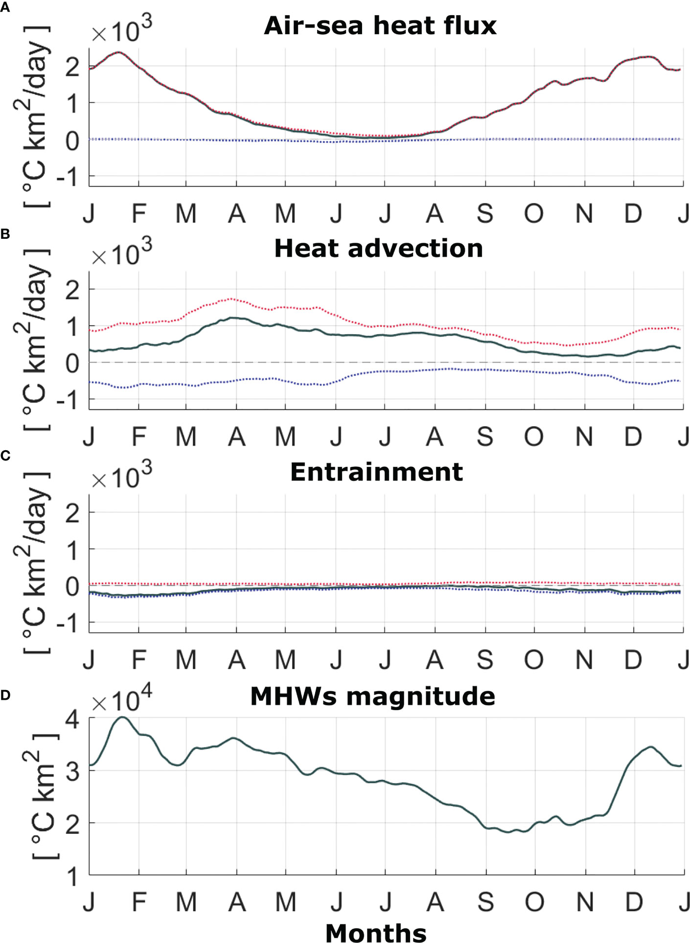
Figure 3 Annual cycle of the different MHW drivers in the study region. Each driver was integrated over the spatial extent impacted by a MHW, then the daily values, corresponding to the same calendar day, were averaged over the 1993-2018 period. Air-sea heat fluxes (A), heat advection (B), entrainment (C) and magnitude of MHWs (D). The black curves in (A–C) show the average of all values, while the red lines show the average of only positive values (contribution to warming), and the blue lines show the average of the negative values (contribution to cooling).

Figures 3A–C also show the contribution of the different terms of (1), distinguishing their positive (red curves) and negative (blue curves) contributions to the heat balance. The positive (negative) contribution of the driver occurs when only values favorable to the warming (cooling) of the driver are considered. This allows better analysis of the nature of the MHW in the region. For instance, a MHW event could be dominated by two different mechanisms in different subareas within the study region, and the same driver can be adding and subtracting heat from the surface layer within different subareas of the same MHW, which would result in a rather small total effect of the driver after averaging over the whole region affected by the MHW. In such cases, the double nature of the MHW would be missed. In summary, the climatological heat balance within the MHWs showed that ASHFs practically always contribute to increasing surface layer temperature (i.e., the red and black lines are similar in Figure 3A), whereas HA shows both positive and negative contributions –represented in Figure 3C by red and blue lines, respectively– with a predominance of positive values (black line). Entrainment plays only a secondary role and commonly contributes to reducing MLT. Then, the main drivers of the MHWs are HA and ASHFs.

Daily anomalies of ASHFs, HA, and entrainment vary widely within the MHWs, with fluctuations that are about one order of magnitude larger than the amplitude of their seasonal cycle (Figure 4 and Figure S3 in Supporting Information). The red line shows the standard deviation, which was calculated using a moving window of 365 days (using this moving window, we avoid overweighting the influence of ENSO). The values over each red line correspond to periods when the drivers are more important; these periods are used to illustrate the specific processes associated with the different drivers. Note that most of the peaks in the ASHF and HA anomalies (Figures 4A, B) are related to El Niño. This phenomenon is most evident in the extreme events of 1997-1998 and 2015-2016, but the impact of the “Coastal El Niño” is also clearly visible during the austral summer of 2017.In general, the spatial pattern of the HA anomalies (Figure 5A) resembles the observed MHW patterns of both frequency and duration (Figures 1A, B). These patterns result from the combination of ASHF and HA. Despite the ASHF is the main driver of most MHWs, the HA has more spatial structure in the oceanic region than the relatively homogenous ASHF pattern (see Figure 7A below). Note that there are periods not related to ENSO when HA and ASHF anomalies are larger than their respective threshold red curves.

FIGURE 4

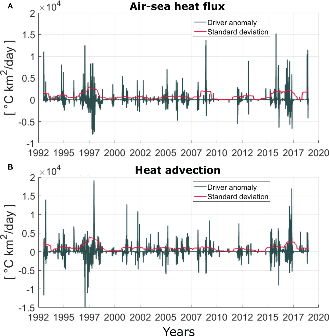
Figure 4 MHW driver anomalies (respect to their seasonal cycle) integrated over the spatial extent and periods affected by MHWs in the study region (see black contour in Figure 1). Air - sea heat fluxes (A), and heat advection (B). The red line indicates the value of one standard deviation calculated inside of a 365-day moving window. Days exceeding this standard deviation were used to calculate and classify the warming mechanism (drivers) associated with the MHWs.

FIGURE 5

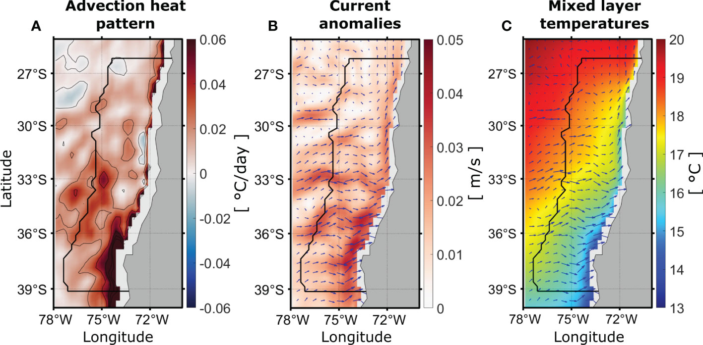
Figure 5 Warming related to heat advection (A). These values were calculated by averaging the HA (°C day^-1) during the days that HA was larger than the threshold value shown by the red line in Figure 4B. Mean pattern of the associated current anomalies (B) and temperature of the mixed layer (C) (also current anomalies are shown by arrows). The black contours show the study region.

During El Niño, the magnitude of MHWs (mean value ~6.9×10⁴°C km²) is greater than during La Niña (mean value ~5.7x10^4° km²) and neutral periods (mean value ~4.3x10⁴ km²) (Figure 6A). Interestingly, the magnitude of MHWs during La Niña is greater than during neutral conditions (Figures 6C, D). During El Niño, the most intense MLT anomalies are observed near the coast (Figure 6B), whereas during La Niña, larger magnitudes are present in the offshore region (Figure 6C). In summary, ENSO cycles increase the probability of more intense MHWs in our study region.

FIGURE 6

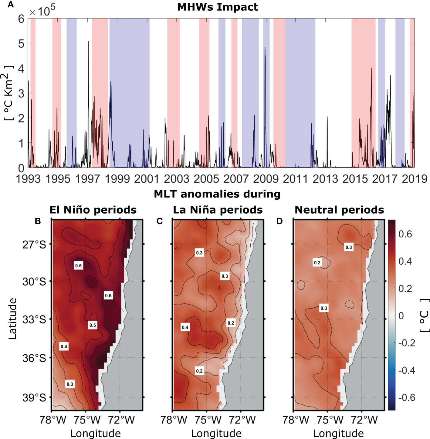
Figure 6 Relationship between MHWs and ENSO. Time series of MHW magnitudes (A), El Niño (La Niña) periods are shaded in red (blue). El Niño and La Niña periods were defined based on the ONI (Oceanic El Niño index https://origin.cpc.ncep.noaa.gov/products/analysis_monitoring/ensostuff/ONI_v5.php). Mean spatial patterns of MLT anomalies observed during periods affected by MHWs (magnitude of MHWs > 0) and concomitant to El Niño (B), La Niña (C), and ENSO-neutral conditions (D). The most intense MLT anomalies are observed during El Niño periods, and these are larger near the coast. MLT anomalies during La Niña are smaller than during El Niño periods, but higher than during neutral periods, showing larger magnitudes in the offshore region.

The warming pattern (in °Cd^-1) related to the ASHFs shows positive values across the region. Larger values are found near the coast (Figure 7A), where the mixed layer is shallower (Figure 7B).Among the different terms involved in the air-sea heat exchange (Figure 8), the term related to latent heat flux (Figure 8C) is the most relevant in creating the spatial pattern observed in Figure 7A. In contrast to the pattern observed from the latent heat flux anomalies (Figure 8C), patterns of short and longwave radiation anomalies show mainly meridional variability and smaller magnitude (Figures 8A, B). The sensible heat flux anomalies are spatially more homogeneous and slightly positive (Figure 8D).

FIGURE 7

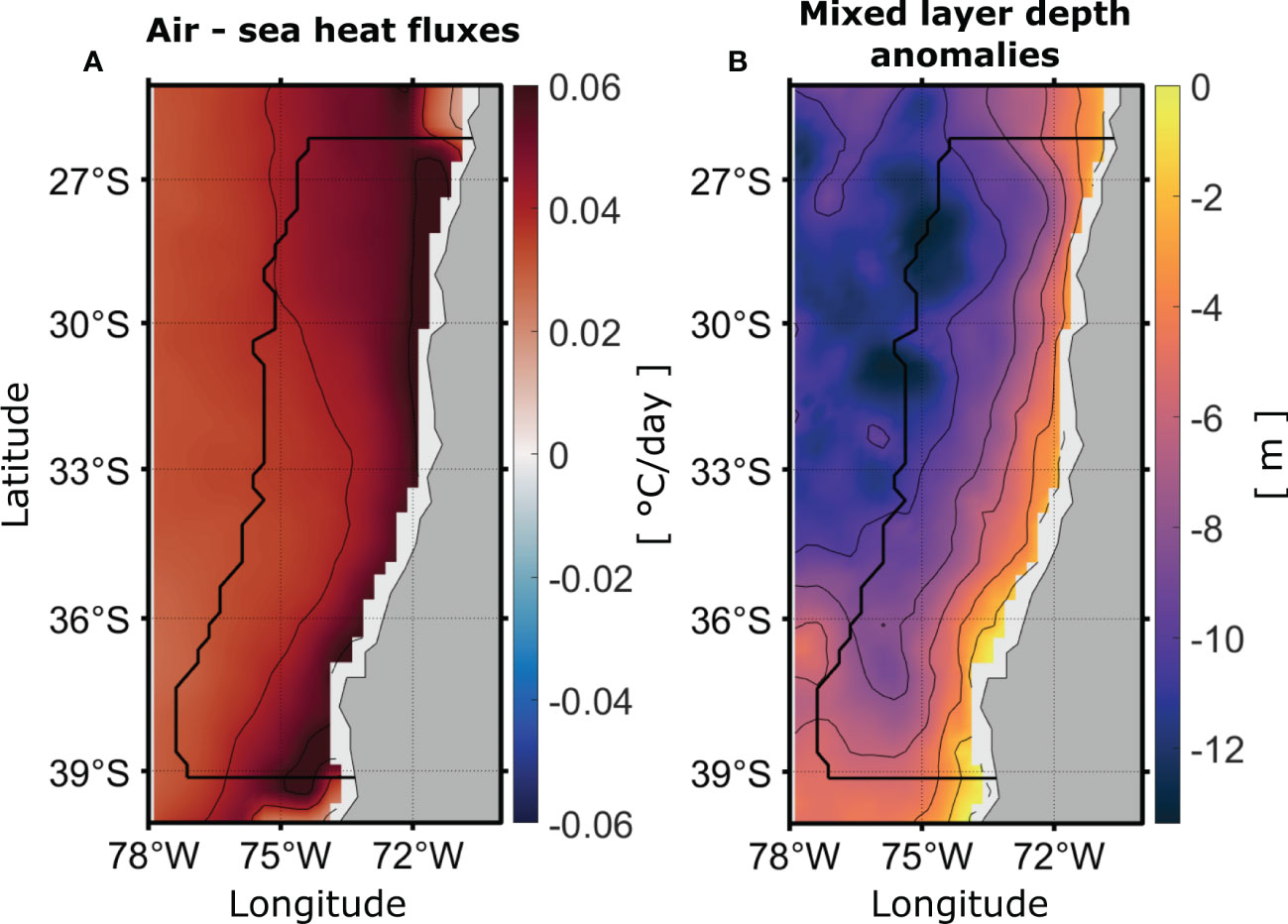
Figure 7 Mean magnitude of the warming generated by air-sea heat fluxes (A), and mixing layer depth anomalies (B). The selected days to calculate the air-sea heat fluxes correspond to days where the fluxes exceed the threshold value shown by the red line in Figure 4A. The black contours show the study region.

FIGURE 8

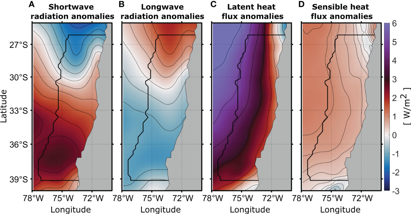
Figure 8 Mean magnitude of the different air-sea heat fluxes when ASHF are relatively high (over their threshold value Figure 4A) between 1993 and 2018. Shortwave radiation anomalies (A), longwave radiation anomalies (B) latent heat flux anomalies (C) and sensible heat flux anomalies (D). Anomalies are positive when the heat flow is toward the ocean. The black contours show the study region.

The spatial pattern of the HA (Figure 5A, in °C/d) shows that all the region tends to be warmed up by this driver, but the largest values are observed along a narrow coastal band. This warming is more intense south of 32°S, affecting a larger offshore region. The warming pattern is related to both eastward (onshore) current anomalies and a large zonal temperature gradient in all the region, being more intense south of 32°S (Figure 5B, C). It is worth noting that the HA is, in general, smaller than the ASHF in our study region and entertainment anomalies are commonly much smaller (<8%). As stated before, a MHW could be generated and maintained by different drivers acting at different times and places. Most long MHWs are driven by a combination of ASHF and HA.

3.3 The 1997-1998 and 2016-2017 MHWs

To better illustrate our results, we analyze two extreme MHWs: one during 1997-1998, related to the large El Niño event, and the other during 2016-2017, related to the “coastal El Niño”. The 1997-1998 El Niño was the strongest on record (e.g., McPhaden, 1999) and generated the most extreme and longest MHW observed in our study region (Figure 2). During this MHW, both HA and ASHFs were relevant. Previous to the 1997-1998 El Niño, during January-February, a MHW impacted the region (Figure 9A). Its growth was initially driven by an increase in ASHFs (Figure 9C), whereas the contribution of HA remained relatively low. After that, the magnitude of the MHW dropped nearly to 0 but remained positive. During April-June 1997, the magnitude of the MHW began to grow again (Figure 9A) related to the onset of the strong El Niño in the region (Ulloa et al., 2001). At that time, the HA increased considerably (Figure 9B), whereas the magnitude of ASHFs was close to zero. In austral winter, the ASHFs started increasing and peaked in November 1997 (Figure 9C), contributing to maintaining the long MHW observed in our region. Then, in December 1998, near the peak of the ENSO event, both ASHF and HA increased (Figures 9B, C). Thus, the extreme MHW of 1997-1998 observed off central Chile was driven by a combination of ASHF and HA. The pattern of the ASHFs term shows that during January-February 1997, ASHFs contributed to the MHW in most of the offshore region (Figure 9E). Then, during the onset of the 1997-1998 El Niño (April-June 1997), HA was the dominant driver with intensity showing a variable spatial pattern in the offshore region (Figure 9F). In contrast, during December 1997, the HA dominated very close to the coast increasing the MHW intensity (Figure 9G). This last pattern is consistent with large coastal trapped waves –forced by equatorial Kelvin waves– arriving in central Chile (e.g., McPhaden and Yu, 1999). In addition, the ASHF also made an important contribution in December 1997, similar to the previous period (August-November 1997), with a similar warming pattern (Figure 9H). Prior to the 1997-1998 El Niño, in January-February 1997, a large MHW impacted the region (Figure 9A). This MHW was mainly driven by ASHF, with a minor contribution from HA (Figures 9B, C). During this period, satellite SST data showed positive anomalies over a wide region of the South Pacific centered around 30°-35°S, reaching the coast of central Chile (c.f., Shaffer et al., 1999).

FIGURE 9

Figure 9 MHW observed off central Chile during the 1997-1998 El Niño event. Time series in (A) shows the magnitude of this MHW, the first period was dominated by ASHFs during early 1997 (left yellow shading), the second period was dominated by HA during mid 1997 (central yellow shading), and the third period was dominated by the combination of both drivers (late 1997, right yellow shading). Time series of HA (B), ASHFs (C) and entrainment (D). The time series were obtained by integrating the drivers over the region affected by the MHW within the study region (black contour). Warming pattern produced by ASHFs during early 1997 (E) and during late 1997 (H) corresponding to the period shaded in yellow in (A). Warming pattern produced by HA during mid 1997 (F) and late 1997 (G).

During the coastal El Niño of 2016-2017, a large MHW occurred off central Chile (Figure 10). In November and December 2016, ASHF dominated the surface heat budget, driving this MHW (Figures 10A, C first yellow-shaded period). The spatial pattern of ASHF-related warming in this period is intense and relatively homogeneous, affecting the whole zone (Figure 10D). Later, both ASHF and HA become relevant in supporting this MHW (Figures 10A–C; gray-shaded period). This occurs simultaneously with the maximum expressions of coastal El Niño. During the last stage of this MHW, the HA was stronger and dominated the heat balance (Figures 10A, B April-May 2017; second yellow-shaded period). Finally, HA and MHW decay together during mid-2017. The heating pattern generated by HA during this last period shows large mesoscale variability with strong warming nuclei, mostly near the coast (Figure 10G).

FIGURE 10

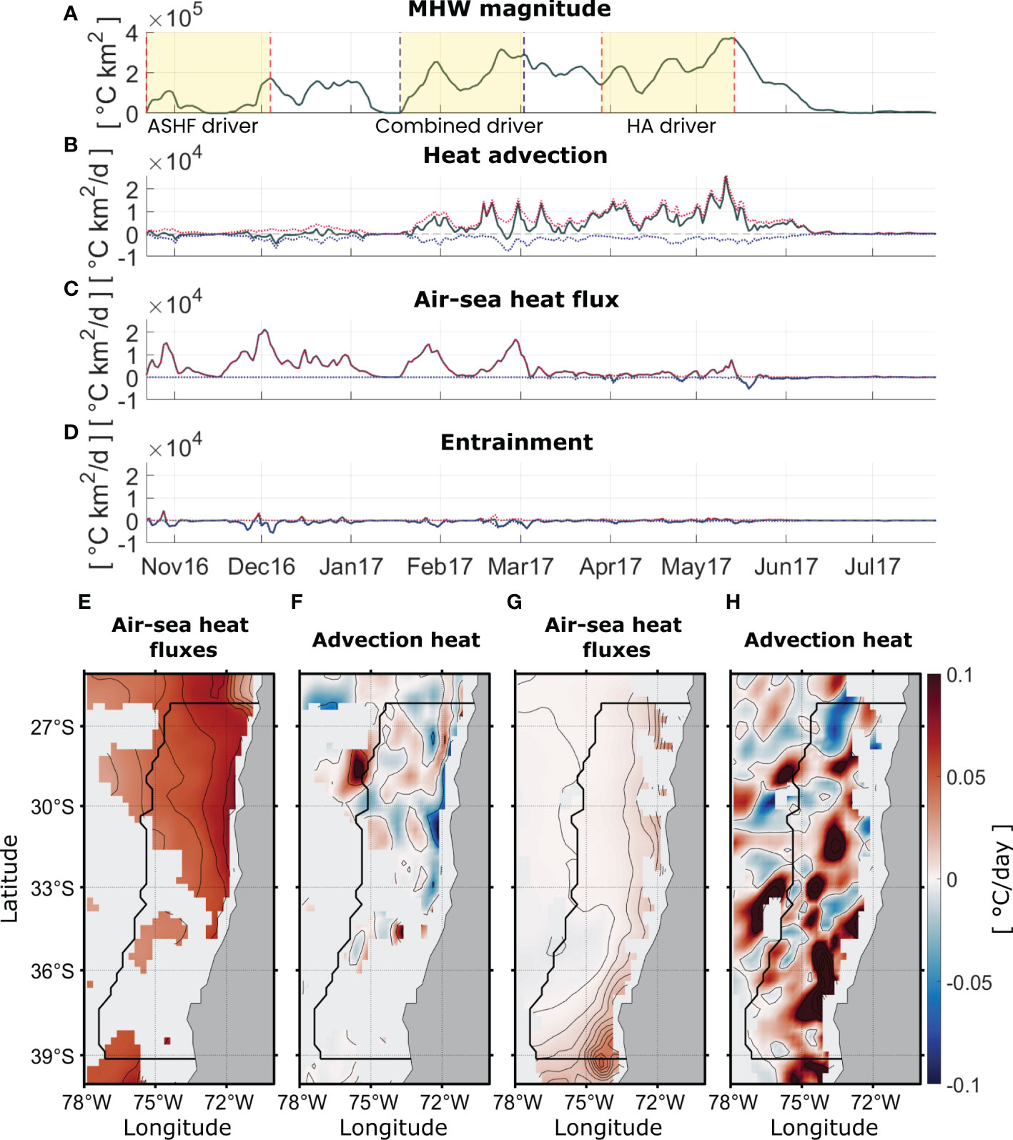
Figure 10 MHW generated by a combination of both, air-sea heat fluxes and heat advection, occurring between late 2016 and early 2017. The time series (A) shows the magnitude of the MHW, the first period was dominated by air-sea heat fluxes at the end of 2016 (yellow shading), a second period was dominated by combined drivers (gray shading) and a third period was dominated by heat advection (yellow shading at the right). Time series of the HA integrated in the MHW region (B). Time series of ASHFs (C) and time series of entrainment (D). The time series were obtained by integrating the drivers over the region affected by the MHW within the study region (black contour). Warming spatial pattern associated with ASHFs during the first part of the MHW (yellow shading centered on Nov 2016) (E) and during the third period (yellow shading centered on Apr 2017) (G). Warming pattern produced by HA during the first period (yellow shading centered on Nov 2016) (F) and during the third period (yellow shading centered on Apr 2017) (H).

3.4 Comparing the different types of observed MHW

Based on the main drivers, we can distinguish three types of MHW: 1) mainly forced by ASHF, 2) mainly forced by HA, and 3) combined-type, in which the relevance of both ASHF and HA is similar. Figure 11 presents a summary of the classification of MHWs. ASHF-type MHWs were the most frequent –more than 65 out of 147 events (44%) were observed in our 26-year-long study period (Figure 11A). These MHWs had a mean intensity of ~1.2°C and a maximum intensity of ~2.5°C (Figure 11C). For those MHWs that are dominated by a particular driver, HA exhibits a higher mean partial contribution to the total magnitude than ASHF (in average, 814 vs 605°C km² day^-1, respectively). During ASHF-type MHWs, the mixed layer is considerably reduced, reaching a typical depth of only ~18 m (Figure 11D). Thus, ASHFs can warm up more quickly in a region with a reduced mixed layer, making this driver more efficient to increase the MLT. This type of MHWs occurs when the wind is reduced, thus decreasing the mixing in the surface layer and, in turn, the MLD. ASHF-type MHW are characterized by a relatively short duration, ~24 days (Figure 11B), whereas their average spatial extent covers ~2.8×10⁴ km² (Figure 11D). The largest MHW of this type impacted ~34% of the whole study region on average.

FIGURE 11

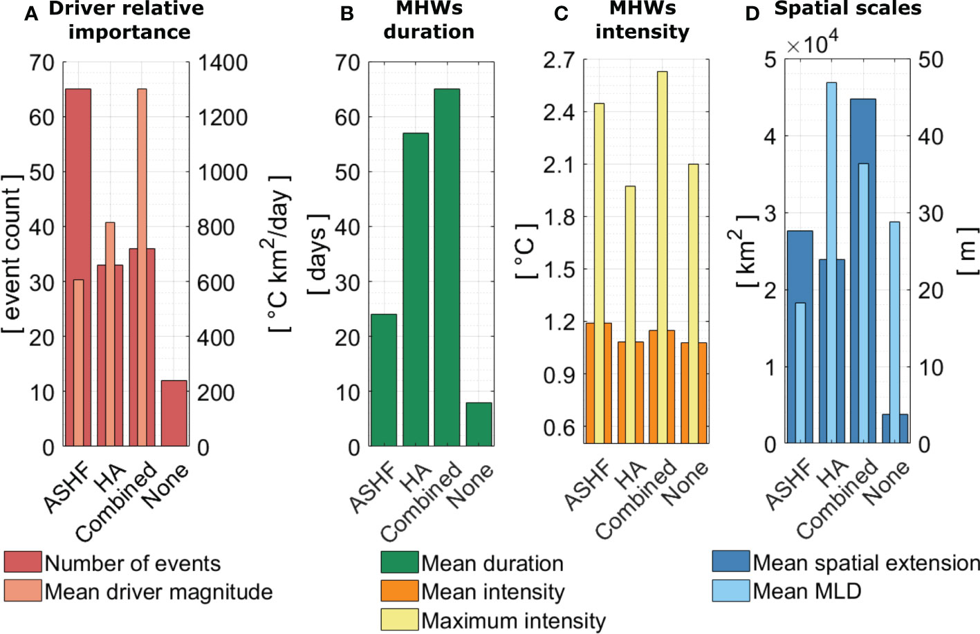
Figure 11 Representation of the dominant drivers of the MHWs and their characteristics off central Chile: (A) Number of events dominated by the different drivers (thick bars and left axis) and mean magnitude of the corresponding driver (thin bars and right axis). (B) Mean duration of the MHW related to the different driver types. (C) Mean intensity (thick bars) and maximum intensity (thin bars) of the MHW. (D) Averaged spatial extension (thick bars and left axis) and depth of the mixed layer (thin bars and right axis) related to the different type of MHWs. None corresponds to those MHWs that are not dominated by any specific driver according to the selected criteria to define the different MHW types. We include the MLD in panel D to clarify why a driver with less magnitude (e.g., ASHF) may lead to more intense MHWs (for instance, in HA-type MHWs the MLD is commonly more than twice the MLD observed in ASHF-type, that involve that the HA driver is commonly less efficient to rise the mixed layer temperature).

The HA-type MHWs are considerably less frequent (Figure 11A): only 33 out of 147 (23%) events of this MHW occurred during the study period. As stated above, the partial contribution of HA to the total magnitude is on average ~814°C km² day^-1 during HA-type MHWs, which is larger than the partial contribution of air-sea heat fluxes during the ASHF-type MHWs. However, in this case, the mixed layer is thicker (~47 m depth) (Figure 10D). These MHWs have smaller maximum (~2.0°C) and slightly smaller mean intensities (~1.1°C on average) compared with the other MHW-types (Figure 11C). The mean duration of AH-type MHWs is ~57 days, about twice the mean duration of the ASHF-type MHWs. Moreover, their average spatial extent involves an area of ~2.4×10⁴ km² (Figure 11D), including a particular MHW that reached an average extension of 27% of the entire region analyzed.

During the study period, 36 combined-type MHWs were observed, representing 25% of the total 147 events. Hence, this group is more (less) frequent than HA-type (ASHF-type) MHWs (Figure 11A). The combined-type MHWs showed a mean intensity of ~1.2°C and maximum intensities (~2.6°C) similar to the ASHF-type MHW (Figure 11C). The mean partial contribution of the combined heat fluxes (ASHF + HA) to the total magnitude was 650°C km² day^-1 (Figure 11A). These MHWs had the longest duration (~65 days) (Figure 11B). As shown in the study cases above, the different drivers may act simultaneously or during different periods, thus extending the MHW duration. Consequently, combined-type MHWs had the largest spatial extents (~4.5×10⁴ km² (Figure 11D), being considerably superior to the other two types of MHWs. The largest MHW reached an average spatial extent of about 39% of the entire region and corresponded to the event observed during the 1997-1998 El Niño, analyzed in the previous section. The MLD during this type of MHW was on average ~36 m (Figure 11D), an intermediate value between those for the other two types. Finally, MHWs that do not exhibit a main contribution by the drivers analyzed presented the lowest frequency: only 12 events out of 147, i.e., 8%. They were generally weaker than the MHWs analyzed above (Figures 9 and 10), showed the shortest duration (~8 days on average) (Figure 11B), and the smallest spatial extensions (~0.4×10⁴ km²) (Figure 11D).

4 Discussion and summary

Here we use reanalysis products –GLORYS-2V4 and ERA-interim– to describe MHWs off central Chile and to analyze their main driving mechanisms. Our results show that ASHF and HA are the main drivers of these events; the relative contribution of these drivers define three types of MHWs, namely: ASHF-type, AH-type, and combined-type. Entrainment does not play a relevant role driving MHWs in the study region. In general, the coastal region off Chile is characterized by relatively low temperatures due to the upwelling of cold waters during most of the year (e.g., Strub et al., 2013). Consistently, Pietri et al. (2021) found that most MHWs shorter than 100 days off Peru are associated with a weakness of upwelling-favorable winds and so with reduction of entrainment of cold waters near the coast. Nevertheless, our results showed that the entrainment is not clearly reduced during MHW. Rather, it usually continues rather normal and the frequency of MHWs do not exhibit a clear contrast between the coastal and the oceanic regions (Figure 1). However, the mean duration of MHWs is smaller and intensity is larger near the coast of central Chile (Figure 1B). It is worth noting that entrainment was estimated from the wind field and other phenomena like baroclinic coastal trapped waves may also play a significant role near the coast. According to Varela et al. (2021), MHWs off Chile show different trends between the oceanic and coastal regions, being principally negative near the coast. Their analysis was based on SST (NOAA OISST) for the period 1982-2018. The GLORYS product has relatively good temporal (daily), horizontal and vertical (particularly in the upper ocean) resolutions to perform a heat balance in the mixed layer. The MHWs estimated from GLORYS have a very good agreement with the NOAA OISST product. A product commonly used in MHW’s studies, both globally and regionally in the eastern South Pacific (e.g., Hobday et al., 2018; Pietri et al., 2021; Pujol et al., 2022). We also compare MHWs based on GLORYS/ERA-interim with those estimated using in situ observations from the Stratus buoy near 21°S 85°W (https://uop.whoi.edu/ReferenceDataSets); both results were quite consistent (not shown here).

El Niño events have a strong impact on SST off central Chile (e.g., Shaffer et al., 1999; Hormazabal et al., 2001; Escribano et al., 2004). In fact, we observed the highest MLT anomalies related to the MHWs in these periods (Figure 5A). Although the effects differ for different events –e.g., central and eastern El Niño events (Takahashi et al., 2011)–, the typical anomalies observed during El Niño periods exceed 2°C near the coast of central Chile (Enfield, 2001; Escribano et al., 2004). In this region, the SST anomalies related to El Niño result from a complex interaction of different oceanographic and atmospheric processes: (1) During El Niño events, downwelling coastal trapped waves –forced by equatorial Kelvin waves that hit the South American coast– deepen the thermocline along the coast and, although upwelling of subsurface waters may continue, the upwelled waters are warmer than usual (Huyer et al., 1987; Hormazabal et al., 2001). Low-frequency perturbations of the pycnocline may also propagate offshore, extending the impact of coastal disturbances toward the ocean interior (Vega et al., 2003; Ramos et al., 2006). (2) Downwelling coastal trapped waves are also associated with an increase of southward advection of surface warmer water (e.g., Pizarro et al., 2002). Onshore surface current anomalies transporting warm oceanic waters toward the coast have also been observed during El Niño (Huyer et al., 1987). (3) Although regional warming during El Niño is essentially driven by oceanic mechanisms, this also induces atmospheric warming of the air in subtropical and tropical South America (e.g., Garreaud et al., 2009). In addition to El Niño, La Niña also has a great impact on SST off central Chile (Figure 6B) compared to periods not affected directly by ENSO (Figure 6C). Both El Niño and La Niña exhibit stronger MHW impacts than ENSO-neutral years (Figure 6A). Thus, we conclude that ENSO cycles have a great capacity to modulate the characteristics of MHWs mainly by impacting HA.

The large MHW observed during 2016-2017 was related to the coastal El Niño. This event triggered extreme coastal warming off Peru, mainly due to a relaxation of the southeasterly trade winds off the coast (Garreaud, 2018; Takahashi et al., 2018). The weakening of the trade winds off Peru decreased the upwelling intensity along the coastal zone and reduced evaporation in a larger offshore region. The coastal 2016-2017 El Niño also triggered severe rains along the west coast of tropical South America, with devastating socio-economic consequences (Rodriguez-Morata et al., 2019).

ASHFs present their greatest magnitude during the warm season (spring and summer), generating a large number of MHWs. Hence, ASHF-type MHWs are the most frequent in our study region. The warming induced by ASHFs affects the whole region with a similar magnitude (Figure 7A). During MHWs, ASHFs do not induce cooling. The main characteristics of ASHF-type MHWs are their high frequency (65 out of 147 events), mean intensity of ~1.2°C, maximum intensity reaching ~2.5°C, spatial extension up to 34% of the entire study region, and short duration (less than one month). In the cold season (autumn and winter), the magnitude of the ASHFs is greatly reduced, and the probability of the generation of ASHF-type MHWs in these periods strongly decreases. This type of events are mainly generated by heightened solar radiation or decreased evaporation, which can occur separately or together at different locations and times within the development of a MHW.

HA-type MHWs are generated mainly by eastward current anomalies superimposed on a mean westward temperature gradient ( $u^{\prime }\partial \overline{T}/\partial x$ which dominates in the term $v·\nabla \overline{T}$). Note that while $v^{\prime }·\nabla \overline{T}$tends to increase the MLT, the nonlinear term ( $v^{\prime }·\nabla {\overline{T}}^{\prime }$)tends to reduce the MLT, and $v^{\prime }·\nabla {\overline{T}}^{\prime }$ is, in general, much smaller than the other two terms shown above. HA presents its highest magnitude during autumn but is also relatively high in summer and winter. It makes a considerable contribution to warming in all seasons, indicating that these MHWs may occur year round. During MHWs, HA contributes much less to cooling than to warming. Nevertheless, considerably intense cooling takes place in summer and autumn. This fact supports a large variability of the HA term (as observed for the MHWs analyzed in previous sections). The main characteristics of advective-type MHW are low frequency (compared to ASHF events), mean intensity of ~1.1°C, maximum intensity up to ~2°C, spatial extent reaching a maximum of 27% of the study region, and long duration (about two months).

The most intense MHWs generally occur close to the coast, which is consistent with the fact that the warming signal caused by their main drivers (ASHF and HA) is also stronger towards the coast. The most intense MHWs are those grouped within the combined type. In these cases, the warming contributions induced by HA and ASHFs are observed concomitantly or during different periods or subareas within a certain MHW. The main characteristics of combined-type MHWs are a slightly higher (significantly lower) frequency than HA (ASHF) events, mean intensity of ~1.2°C, maximum intensity reaching ~2.6°C, and the largest spatial extension, impacting up to 39% of the whole study region. Their mean duration is slightly longer than the advective events (more than two months).

In this study, we analyzed the main properties and drivers of the MHWs in the eastern South Pacific off central Chile. Most studies mainly focus on the impacts of large SST anomalies related to El Nino events, while ecological effects of all MHWs should also be of importance. Different kinds of MHWs involve environmental changes that can directly impact pelagic species that are relevant to large- and small-scale fisheries, as well as kelp forests that are key to biodiversity of coastal zones (e.g., Arafeh-Dalmau et al., 2020; Cheung and Frölicher, 2020). In our region, small-scale fisheries and harvesting of wild seaweed are highly sensitive to temperature distribution and contribute significantly to the total catches of the country and to the livelihood of multiple coastal communities (e.g., Villegas et al., 2019; Chevallier et al., 2021). Here we have identified the main properties and drivers of the MHWs observed off central Chile in the last decades. Nevertheless, the evaluation of the impacts of different types of MHWs on the pelagic and coastal environments is an important task that needs to be addressed in future studies. In addition to the impacts on the marine environment, MHWs may also be related to extreme weather events of northern Chile. A dramatic example is the large floods observed in March 2015 in northern Chile (resulting in significant damage and several casualties), which was closely related to a MHW over the eastern Pacific (Bozkurt et al., 2016).

The long MHWs that occur during El Niño periods in the study region have traditionally been associated with warm water advection and the role of ASHF has been commonly underestimated. However, our results show that the large and prolonged heat waves during the 1997-98 El Niño event did not only result from warm water advection, but from a combination of ASHF and HA. On the other hand, ASHF-type MHW are the most frequent during non-El Niño years, and they are even more common during La Niña than during ENSO-neutral years. These heat waves are closely associated with a reduction of MLD, a difficult variable to simulate by numerical models (e.g., Oschlies, 2002; Fox-Kemper et al., 2008). In general, to build realistic forecasts of extreme events associated with MHWs together with adequate information from ASHF and HA, it is necessary to improve our ability to estimate the MLD off the coast of Chile.

Data availability statement

Publicly available datasets were analyzed in this study. This data can be found here: https://doi.org/10.48670/moi-00024 https://www.ecmwf.int/en/forecasts/datasets/reanalysis-datasets/era-interim.

Author contributions

DC and OP designed the study and methodology. DC and OP wrote the manuscript with contribution of all authors, DC performed the data analysis and produced the figures. OP, MJ-C and DN supervised the research, refined the methodology and contributed to the interpretation of the results. All authors contributed to the article and approved the submitted version.

Funding

This work was supported by ANID (FONDECYT projects: 11811872 leaded by OP). The first author, DC, received support by a magister scholarship from the Millennium Institute of Oceanography (IMO), Chile. This work was also partially funded by IMO (ANID, ICM grant IC-120019), Programa de Centros Regionales (ANID/2020-R20F0008-CEAZA), COPAS COASTAL (ANID/FB210021) and the Centre for Climate and Resilience Research (CR)2 (ANID/FONDAP/1522A0001).

Conflict of interest

The authors declare that the research was conducted in the absence of any commercial or financial relationships that could be construed as a potential conflict of interest.

Publisher’s note

All claims expressed in this article are solely those of the authors and do not necessarily represent those of their affiliated organizations, or those of the publisher, the editors and the reviewers. Any product that may be evaluated in this article, or claim that may be made by its manufacturer, is not guaranteed or endorsed by the publisher.

Supplementary material

The Supplementary Material for this article can be found online at: https://www.frontiersin.org/articles/10.3389/fmars.2023.1129276/full#supplementary-material

References

Arafeh-Dalmau N., Schoeman D. S., Montaño-Moctezuma G., Micheli F., Rogers-Bennett L., Olguin-Jacobson C., et al. (2020). Marine heat waves threaten kelp forests. Science 367 (6478), 635–635. doi: 10.1126/science.aba5244

PubMed Abstract | CrossRef Full Text | Google Scholar

Berrisford P., Kållberg P., Kobayashi S., Dee D., Uppala S., Simmons A. J., et al. (2011). Atmospheric conservation properties in ERA-interim. Q. J. R. Meteorol. Soc. 137 (659), 1381–1399. doi: 10.1002/qj.864

CrossRef Full Text | Google Scholar

Bond N. A., Cronin M. F., Freeland H., Mantua N. (2015). Causes and impacts of the 2014 warm anomaly in the NE pacific. Geophys. Res. Lett. 42 (9), 3414–3420. doi: 10.1002/2015gl063306

CrossRef Full Text | Google Scholar

Bozkurt D., Rondanelli R., Garreaud R., Arriagada A. (2016). Impact of warmer eastern tropical pacific SST on the march 2015 atacama floods. Monthly Weather Rev. 144 (11), 4441–4460. doi: 10.1175/MWR-D-16-0041.1

CrossRef Full Text | Google Scholar

Caputi N., Kangas M., Denham A., Feng M., Pearce A., Hetzel Y., et al. (2016). Management adaptation of invertebrate fisheries to an extreme marine heat wave event at a global warming hot spot. Ecol. Evol. 6 (11), 3583–3593. doi: 10.1002/ece3.2137

PubMed Abstract | CrossRef Full Text | Google Scholar

Cavole L., Demko A., Diner R., Giddings A., Koester I., Pagniello C., et al. (2016). Biological impacts of the 2013–2015 warm-water anomaly in the northeast pacific: Winners, losers, and the future. Oceanography 29 (2), 273–285. doi: 10.5670/oceanog.2016.32

CrossRef Full Text | Google Scholar

Chelton D. B., DeSzoeke R. A., Schlax M. G., El Naggar K., Siwertz N. (1998). Geographical variability of the first baroclinic rossby radius of deformation. J. Phys. Oceanog. 28 (3), 433–460. doi: 10.1175/1520-0485(1998)028%3C0433:gvotfb%3E2.0.co;2

CrossRef Full Text | Google Scholar

Cheung W. W., Frölicher T. L. (2020). Marine heatwaves exacerbate climate change impacts for fisheries in the northeast pacific. Sci. Rep. 10 (1), 1–10. doi: 10.1038/s41598-020-63650-z

PubMed Abstract | CrossRef Full Text | Google Scholar

Chevallier A., Broitman B. R., Barahona N., Vicencio-Estay C., Hui F. K., Inchausti P., et al. (2021). Diversity of small-scale fisheries in Chile: Environmental patterns and biogeography can inform fisheries management. Environ. Sci. Policy 124, 33–44. doi: 10.1016/j.envsci.2021.06.002

CrossRef Full Text | Google Scholar

Dee D. P., Uppala S. M., Simmons A. J., Berrisford P., Poli P., Kobayashi S., et al. (2011). The ERA-interim reanalysis: Configuration and performance of the data assimilation system. Q. J. R. meteorol. Soc. 137 (656), 553–597. doi: 10.1002/qj.828

CrossRef Full Text | Google Scholar

Dewitte B., Conejero C., Ramos M., Bravo L., Garcon V., Parada C., et al. (2021). Understanding the impact of climate change on the oceanic circulation in the Chilean island ecoregions. Aquat. Conservat.: Mar. Freshw. Ecosyst. 31 (2), 232–252. doi: 10.1002/aqc.3506

CrossRef Full Text | Google Scholar

Di Lorenzo E., Mantua N. (2016). Multi-year persistence of the 2014/15 north pacific marine heatwave. Nat. Climate Change 6 (11), 1042–1047. doi: 10.1038/nclimate3082

CrossRef Full Text | Google Scholar

Echevin V., Colas F., Espinoza-Morriberon D., Vasquez L., Anculle T., Gutierrez D. (2018). Forcings and evolution of the 2017 coastal El niño off northern Peru and Ecuador. Front. Mar. Sci. 5. doi: 10.3389/fmars.2018.00367

CrossRef Full Text | Google Scholar

Enfield D. B. (2001). Evolution and historical perspective of the 1997–1998 El niño–southern oscillation event. Bull. Mar. Sci. 69 (1), 7–25.

Google Scholar

Escribano R., Daneri G., Farías L., Gallardo V. A., González H. E., Gutiérrez D., et al. (2004). Biological and chemical consequences of the 1997–1998 El niño in the Chilean coastal upwelling system: a synthesis. Deep Sea Res. Part II: Top. Stud. Oceanog. 51 (20-21), 2389–2411. doi: 10.1016/j.dsr2.2004.08.011

CrossRef Full Text | Google Scholar

Falvey M., Garreaud R. D. (2009). Regional cooling in a warming world: Recent temperature trends in the southeast pacific and along the west coast of subtropical south America, (1979–2006). J. Geophys. Res.: Atmosph. 114 (D4) D04102, 1–16. doi: 10.1029/2008jd010519

CrossRef Full Text | Google Scholar

Fox-Kemper B., Ferrari R., Hallberg R. (2008). Parameterization of mixed layer eddies. part I: Theory and diagnosis. J. Phys. Oceanog. 38 (6), 1145–1165. doi: 10.1175/2007JPO3792.1

CrossRef Full Text | Google Scholar

Frölicher T. L., Fischer E. M., Gruber N. (2018). Marine heatwaves under global warming. Nature 560 (7718), 360–364. doi: 10.1038/s41586-018-0383-9

PubMed Abstract | CrossRef Full Text | Google Scholar

Frölicher T. L., Laufkötter C. (2018). Emerging risks from marine heat waves. Nat. Commun. 9 (1), 1–4. doi: 10.1038/s41467-018-03163-6

PubMed Abstract | CrossRef Full Text | Google Scholar

Garreaud R. D. (2018). A plausible atmospheric trigger for the 2017 coastal El niño. Int. J. Climatology 38, e1296-e1302. doi: 10.1002/joc.5426

CrossRef Full Text | Google Scholar

Garreaud R. D., Vuille M., Compagnucci R., Marengo J. (2009). Present-day south american climate. Palaeogeog. Palaeoclimatol. Palaeoecol. 281 (3-4), 180–195. doi: 10.1016/j.palaeo.2007.10.032

CrossRef Full Text | Google Scholar

Garric G., Parent L. (2017) Product user manual for global ocean reanalysis products GLOBAL-REANALYSIS-PHY-001-025. Available at: https://catalogue.marine.copernicus.eu/documents/PUM/CMEMS-GLO-PUM-001-025.pdf.

Google Scholar

Hobday A. J., Alexander L. V., Perkins S. E., Smale D. A., Straub S. C., Oliver E. C., et al. (2016). A hierarchical approach to defining marine heatwaves. Prog. Oceanog. 141, 227–238. doi: 10.1016/j.pocean.2015.12.014

CrossRef Full Text | Google Scholar

Hobday A. J., Oliver E. C., Gupta A. S., Benthuysen J. A., Burrows M. T., Donat M. G., et al. (2018). Categorizing and naming marine heatwaves. Oceanography 31 (2), 162–173. doi: 10.5670/oceanog.2018.205

CrossRef Full Text | Google Scholar

Holbrook N. J., Scannell H. A., Sen Gupta A., Benthuysen J. A., Feng M., Oliver E. C., et al. (2019). A global assessment of marine heatwaves and their drivers. Nat. Commun. 10 (1), 1–13. doi: 10.1038/s41467-019-10206-z

PubMed Abstract | CrossRef Full Text | Google Scholar

Holbrook N. J., Sen Gupta A., Oliver E. C., Hobday A. J., Benthuysen J. A., Scannell H. A., et al. (2020). Keeping pace with marine heatwaves. Nat. Rev. Earth Environ. 1 (9), 482–493. doi: 10.1038/s43017-020-0068-4

CrossRef Full Text | Google Scholar

Hormazabal S., Shaffer G., Letelier J., Ulloa O. (2001). Local and remote forcing of sea surface temperature in the coastal upwelling system off Chile. J. Geophys. Res.: Oceans 106 (C8), 16657–16671. doi: 10.1029/2001jc900008

CrossRef Full Text | Google Scholar

Huyer A., Smith R. L., Paluszkiewicz T. (1987). Coastal upwelling off Peru during normal and El niño times 1981–1984. J. Geophys. Res.: Oceans 92 (C13), 14297–14307. doi: 10.1029/jc092ic13p14297

CrossRef Full Text | Google Scholar

Intergovernmental Panel on Climate Change (IPCC) (2022). “Technical summary,” in The ocean and cryosphere in a changing climate: Special report of the intergovernmental panel on climate change (Cambridge: Cambridge University Press), 39–70. doi: 10.1017/9781009157964.002

CrossRef Full Text | Google Scholar

Jacox M. G., Alexander M. A., Bograd S. J., Scott J. D. (2020). Thermal displacement by marine heatwaves. Nature 584, 82–86. doi: 10.1038/s41586-020-2534-z

PubMed Abstract | CrossRef Full Text | Google Scholar

Marin M., Feng M., Bindoff N. L., Phillips H. E. (2022). Local drivers of extreme upper ocean marine heatwaves assessed using a global ocean circulation model. Front. Climate 4. doi: 10.3389/fclim.2022.788390

CrossRef Full Text | Google Scholar

Marin M., Feng M., Phillips H. E., Bindoff N. L. (2021). A global, multiproduct analysis of coastal marine heatwaves: Distribution, characteristics, and long-term trends. J. Geophys. Res.: Oceans 126 (2), e2020JC016708. doi: 10.1029/2020jc016708

CrossRef Full Text | Google Scholar

McCabe R. M., Hickey B. M., Kudela R. M., Lefebvre K. A., Adams N. G., Bill B. D., et al. (2016). An unprecedented coastwide toxic algal bloom linked to anomalous ocean conditions. Geophys. Res. Lett. 43 (19), 10–366. doi: 10.1002/2016gl070023

CrossRef Full Text | Google Scholar

McPhaden M. J. (1999). The child prodigy of 1997-98. Nature 398 (6728), 559–561. doi: 10.1038/19193

CrossRef Full Text | Google Scholar

McPhaden M. J., Yu X. (1999). Equatorial waves and the 1997–98 El niño. Geophys. Res. Lett. 26 (19), 2961–2964. doi: 10.1029/1999gl004901

CrossRef Full Text | Google Scholar

Newman M., Alexander M. A., Ault T. R., Cobb K. M., Deser C., Di Lorenzo E., et al. (2016). The pacific decadal oscillation, revisited. J. Climate 29 (12), 4399–4427. doi: 10.1175/JCLI-D-15-0508.1

CrossRef Full Text | Google Scholar

Oliver E. C. (2019). Mean warming not variability drives marine heatwave trends. Climate Dynam0 53 (3), 1653–1659. doi: 10.1007/s00382-019-04707-2

CrossRef Full Text | Google Scholar

Oliver E. C., Benthuysen J. A., Bindoff N. L., Hobday A. J., Holbrook N. J., Mundy C. N., et al. (2017). The unprecedented 2015/16 Tasman Sea marine heatwave. Nat. Commun. 8 (1), 1–12. doi: 10.1038/ncomms16101

PubMed Abstract | CrossRef Full Text | Google Scholar

Oliver E. C., Benthuysen J. A., Darmaraki S., Donat M. G., Hobday A. J., Holbrook N. J., et al. (2021). Marine heatwaves. Annu. Rev. Mar. Sci. 13, 1–30. doi: 10.1146/annurev-marine-032720-095144

CrossRef Full Text | Google Scholar

Oliver E. C., Burrows M. T., Donat M. G., Sen Gupta A., Alexander L. V., Perkins-Kirkpatrick S. E., et al. (2019). Projected marine heatwaves in the 21st century and the potential for ecological impact. Front. Mar. Sci. 6. doi: 10.3389/fmars.2019.00734

CrossRef Full Text | Google Scholar

Oliver E. C., Donat M. G., Burrows M. T., Moore P. J., Smale D. A., Alexander L. V., et al. (2018). Longer and more frequent marine heatwaves over the past century. Nat. Commun. 9 (1), 1–12. doi: 10.1038/s41467-018-03732-9

PubMed Abstract | CrossRef Full Text | Google Scholar

Oschlies A. (2002). Improved representation of upper-ocean dynamics and mixed layer depths in a model of the north Atlantic on switching from eddy-permitting to eddy-resolving grid resolution. J. Phys. Oceanog. 32 (8), 2277–2298. doi: 10.1175/1520-0485(2002)032<2277:IROUOD>2.0.CO;2

CrossRef Full Text | Google Scholar

Pearce A. F., Feng M. (2013). The rise and fall of the “marine heat wave” off Western Australia during the summer of 2010/2011. J. Mar. Syst. 111, 139–156. doi: 10.1016/j.jmarsys.2012.10.009

CrossRef Full Text | Google Scholar

Pietri A., Colas F., Mogollon R., Tam J., Gutierrez D. (2021). Marine heatwaves in the Humboldt current system: from 5-day localized warming to year-long El niños. Sci. Rep. 11 (1), 1–12. doi: 10.1038/s41598-021-00340-4

PubMed Abstract | CrossRef Full Text | Google Scholar

Pizarro O., Shaffer G., Dewitte B., Ramos M. (2002). Dynamics of seasonal and interannual variability of the Peru-Chile undercurrent. Geophys. Res. Lett. 29 (12), 22–21. doi: 10.1029/2002gl014790

CrossRef Full Text | Google Scholar

Pujol C., Pérez-Santos I., Barth A., Alvera Azcarate A. (2022). Marine heatwaves offshore central and south Chile: Understanding forcing mechanisms during the years 2016-2017. Front. Mar. Sci. 9. doi: 10.3389/fmars.2022.800325

PubMed Abstract | CrossRef Full Text | Google Scholar

Ramos M., Pizarro O., Bravo L., Dewitte B. (2006). Seasonal variability of the permanent thermocline off northern Chile. Geophys. Res. Lett. 33 (9) L09608, 1–4. doi: 10.1029/2006gl025882

CrossRef Full Text | Google Scholar

Reed D., Washburn L., Rassweiler A., Miller R., Bell T., Harrer S. (2016). Extreme warming challenges sentinel status of kelp forests as indicators of climate change. Nat. Commun. 7 (1), 1–7. doi: 10.1038/ncomms13757

CrossRef Full Text | Google Scholar

Rodríguez-Morata C., Díaz H. F., Ballesteros-Canovas J. A., Rohrer M., Stoffel M. (2019). The anomalous 2017 coastal El niño event in Peru. Climate Dynam0 52 (9), 5605–5622. doi: 10.1007/s00382-018-4466-y

CrossRef Full Text | Google Scholar

Scannell H. A., Pershing A. J., Alexander M. A., Thomas A. C., Mills K. E. (2016). Frequency of marine heatwaves in the north Atlantic and north pacific since 1950. Geophys. Res. Lett. 43 (5), 2069–2076. doi: 10.1002/2015gl067308

CrossRef Full Text | Google Scholar

Sen Gupta A., Thomsen M., Benthuysen J. A., Hobday A. J., Oliver E., Alexander L. V., et al. (2020). Drivers and impacts of the most extreme marine heatwave events. Sci. Rep. 10 (1), 1–15. doi: 10.1038/s41598-020-75445-3

PubMed Abstract | CrossRef Full Text | Google Scholar

Shaffer G., Hormazabal S., Pizarro O., Salinas S. (1999). Seasonal and interannual variability of currents and temperature off central Chile. J. Geophys. Res.: Oceans 104 (C12), 29951–29961. doi: 10.1029/1999jc900253

CrossRef Full Text | Google Scholar

Smale D. A., Wernberg T. (2013). Extreme climatic event drives range contraction of a habitat-forming species. Proc. R. Soc. B: Biol. Sci. 280 (1754), 20122829. doi: 10.1098/rspb.2012.2829

CrossRef Full Text | Google Scholar

Smale D. A., Wernberg T., Oliver E. C., Thomsen M., Harvey B. P., Straub S. C., et al. (2019). Marine heatwaves threaten global biodiversity and the provision of ecosystem services. Nat. Climate Change 9 (4), 306–312. doi: 10.1038/s41558-019-0412-1

CrossRef Full Text | Google Scholar

Strub P. T., Combes V., Shillington F. A., Pizarro O. (2013). “Currents and processes along the eastern boundaries,” in International geophysics, vol. 103. (Academic Press), 339–384. doi: 10.1016/b978-0-12-391851-2.00014-3

CrossRef Full Text | Google Scholar

Takahashi K., Aliaga-Nestares V., Avalos G., Bouchon M., Castro A., Cruzado L., Quispe N, et al. (2018). The 2017 coastal El Niño [in “State of the Climate in 2017”]. Bulletin of American Meteorological Society. 99 (8), S210–S211. doi: 10.1175/2018BAMSStateoftheClimate.1

CrossRef Full Text | Google Scholar

Takahashi K., Montecinos A., Goubanova K., Dewitte B. (2011). ENSO regimes: Reinterpreting the canonical and modoki El niño. Geophys. Res. Lett. 38 (10) L10704, 1–5. doi: 10.1029/2011gl047364

CrossRef Full Text | Google Scholar

Ulloa O., Escribano R., Hormazabal S., Quinones R. A., González R. R., Ramos M. (2001). Evolution and biological effects of the 1997–98 El nino in the upwelling ecosystem off northern Chile. Geophys. Res. Lett. 28 (8), 1591–1594. doi: 10.1029/2000gl011548

CrossRef Full Text | Google Scholar

Varela R., Rodríguez-Díaz L., de Castro M., Gómez-Gesteira M. (2021). Influence of Eastern upwelling systems on marine heatwaves occurrence. Global Planet. Change 196, 103379. doi: 10.1016/j.gloplacha.2020.103379

CrossRef Full Text | Google Scholar

Vega A., du-Penhoat Y., Dewitte B., Pizarro O. (2003). Equatorial forcing of interannual rossby waves in the eastern south pacific. Geophys. Res. Lett. 30 (5) 1197, 1–4. doi: 10.1029/2002gl015886

CrossRef Full Text | Google Scholar

Villegas M., Laudien J., Sielfeld W., Arntz W. (2019). Effect of foresting barren ground with macrocystis pyrifera (Linnaeus) c. agardh on the occurrence of coastal fishes off northern Chile. J. Appl. Phycol. 31 (3), 2145–2157. doi: 10.1007/s10811-018-1657-1

CrossRef Full Text | Google Scholar

Wernberg T., Smale D. A., Tuya F., Thomsen M. S., Langlois T. J., De Bettignies T., et al. (2013). An extreme climatic event alters marine ecosystem structure in a global biodiversity hotspot. Nat. Climate Change 3 (1), 78–82. doi: 10.1038/nclimate1627

CrossRef Full Text | Google Scholar