Forecasting Prorocentrum minimum blooms in the Chesapeake Bay using empirical habitat models

Aquaculturists, local beach managers, and other stakeholders require forecasts of harmful biotic events, so they can assess and respond to health threats when harmful algal blooms (HABs) are present. Based on this need, we are developing empirical habitat suitability models for a variety of Chesapeake Bay HABs to forecast their occurrence based on a set of physical-biogeochemical environmental conditions, and start with the dinoflagellate Prorocentrum minimum (also known as P. cordatum).To identify an optimal set of environmental variables to forecast P. minimum blooms, we first assumed a linear relationship between the environmental variables and the inverse of the logistic function used to forecast the likelihood of bloom presence, and repeated the method using more than 16,000 combinations of variables. By comparing goodness-of-fit, we found water temperature, salinity, pH, solar irradiance, and total organic nitrogen represented the most suitable set of variables. The resulting algorithm forecasted P. minimum blooms with an overall accuracy of 78%, though with a significant variability ~ 30-90% depending on region and season. To understand this variability and improve model performance, we incorporated nonlinear effects into the model by implementing a generalized additive model. Even without considering interactions between the five variables used to train the model, this yielded an increase in overall model accuracy (~ 81%) due to the model’s ability to refine the regions in which P. minimum blooms occurred. Including nonlinear interactions increased the overall model accuracy even further (~ 85%) by accounting for seasonality in the interaction between solar irradiance and water temperature. Our findings suggest that the influence of predictors of these blooms change in time and space, and that model complexity impacts the model performance and our interpretation of the driving factors causing P. minimum blooms. Apart from their forecasting potential, our results may be particularly useful when constructing explicit relationships between environmental conditions and P. minimum presence in mechanistic models.

1 Introduction

Harmful algal blooms (HABs) manifest themselves when aquatic algal species grow to such levels that they negatively affect humans, fish, or other aquatic organisms. Examples of such harmful effects are a critical reduction of the oxygen concentration (Glibert et al., 2018) or the production of toxins that may have a significant effect on human and ecosystem health (Marques et al., 2010). It is therefore important to forecast such blooms so aquaculturists and coastal managers can assess risks to health and take appropriate action, such as delaying shellfish harvest and closing beaches when and where HABs are forecasted.

Various modeling techniques have been proposed to forecast and model HABs [see Anderson et al. (2015) and Franks (2018) for a recent review]. Overall, two main classes of models can be distinguished: mechanistic and statistical models (Flynn and McGillicuddy, 2018; Ralston and Moore, 2020). Mechanistic models for these events are typically constructed using fundamental laws of physics and analytical relationships of physiology, and involve solving a set of (differential) equations that allow the forecast of HABs in time and space (e.g., Wong et al., 2007; Qin and Shen, 2019; Hofmann et al., 2021; Zhang et al., 2021; Li et al., 2022). Conversely, statistical models forecast HABs by constructing empirical relationships based on historical data and linking various environmental conditions to the abundance or probability of occurrence of HABs. A disadvantage of statistical models is that they require large data sets, while a disadvantage of mechanistic models is that they include many model assumptions and thus require a priori insight into the functioning of HABs including specific rate parameters needed to develop the mechanistic model formulations (Kendall et al., 1999). Given the complexity of HABs, statistical models have been preferentially used to forecast HABs to date (Ralston and Moore, 2020). A wide range of statistical models have been proposed, ranging from generalized linear models (GLM) (e.g., Anderson et al., 2010; Singh et al., 2014), generalized additive models (GAM) that allow inclusion of nonlinear (interacting) effects (e.g., Carstensen et al., 2015; Díaz et al., 2016), to more advanced machine learning techniques such as decision trees and support vector machines (Recknagel et al., 1997; Brown et al., 2013; Cruz et al., 2021).

Numerous metrics can be used to assess the performance or goodness-of-fit of such statistical models (Johnson and Omland, 2004; Ding et al., 2018). This is not only crucial to optimize and compare model forecasting skill, but also to ascertain which combination of environmental variables should be included in a given model. The Akaike Information Criterion (AIC) (Akaike, 1998), which combines the maximum likelihood principle and Kullback-Leibler information theory (Kullback and Leibler, 1951; Stoica and Selén, 2004), is a commonly employed technique. The advantage of this method is that it optimizes the likelihood function of the model based on the observations while keeping the model as simple as possible to avoid overfitting and assure the model’s generality. Another less-complicated and broadly utilized metric to quantify the goodness-of-fit when focusing on forecasting models is the model accuracy, which compares the model projections and observations by dividing the number of correct forecasts by the total number of forecasts (Stow et al., 2009). Although AIC and model accuracy have been broadly applied using multiple statistical modeling techniques to calculate goodness-of-fit, the effect of model type on AIC, model accuracy, and the variability of model accuracy through space and time is, as far as the authors are aware, largely unknown.

In this contribution, we apply various statistical models to forecast the likelihood of occurrence of high concentrations or ‘blooms’ of the dinoflagellate Prorocentrum minimum (also known as Prorocentrum cordatum) in the Chesapeake Bay. P. minimum is responsible for massive mahogany tides in the Chesapeake Bay, which typically occur in spring. Shellfish culture failures have been reported at sites where large blooms occurred in several Chesapeake Bay tributaries, and at least one large fish kill and toxicity to scallop larvae has been demonstrated for strains of P. minimum (Hégaret and Wikfors, 2005; Wikfors, 2005). Their blooms also significantly attenuate light and negatively affect the growth conditions of submerged aquatic vegetation (Gallegos and Jordan, 2002; Gallegos and Bergstrom, 2005). We consider two model types: a GLM and GAM. An important motivation of choosing a GLM and GAM analysis is that it allow us to study relationships between environmental variables and the probability of P minimum blooms. We determine the effect of model choice on the AIC and model accuracy, and analyze how the model accuracy changes in time and space. Ultimately, these insights will be used to add P. minimum into our suite of forecasts available on the Chesapeake Bay Environmental Forecasting System website (www.vims.edu/cbefs; Bever et al., 2021).

2 Methodology

Approximately 3,600 in situ observations acquired between 1984-2020 from the Chesapeake Bay are used to construct the statistical models for forecasting the likelihood of P. minimum blooms in the Chesapeake Bay. A bloom is defined here as concentrations greater than 1,000 cells mL⁻¹ (Telesh et al., 2016; Pease et al., 2021). We extract observations of P. minimum cell counts and nineteen corresponding physical biogeochemical parameters that were systematically collected over this period from a large data set. We assume a two-class problem (cf., binomial distribution): we either detect a bloom or no bloom, and apply logistic regression. Because we do not know the optimal combination of environmental variables to forecast P. minimum blooms, we assess more than 16,000 variable combinations and identify the best combination based on the AIC and model accuracy. We start with evaluating the accuracy of a relatively simple GLM (Section 3). In a second step we replace the GLM by a GAM to include nonlinear effects and interactions and analyze the spatial and temporal variability of the model accuracy. Finally, we explain the difference found in AIC and model accuracy when adding nonlinearities, and the insights we gain into how environmental variables affect the probability of P. minimum blooms (Section 4).

2.1 The Chesapeake Bay and in situ observations

The Chesapeake Bay is more than 300 km long, approximately 50 km at its widest point, and has an average water depth of approximately 7 m, ranging from 0-40 m (Figure 1). It is the largest continental estuary in the U.S.A. It has multiple tributaries, of which the Susquehanna River, located at the northern boundary, is responsible for nearly 50% of the total freshwater input. The Potomac and James rivers have the second highest freshwater discharge (St-Laurent et al., 2020). The salinity ranges from 0 in the upper tributaries to more than 30 near the mouth. The estuary’s watershed is densely populated and is thus severely anthropologically-impacted (Kemp et al., 2005), resulting in high nutrients loads of, for example, nitrogen (Shenk and Linker, 2013). This stimulates phytoplankton growth, which may increase hypoxic (O₂< 2 mg L⁻¹) volumes from zero in winter to volumes of the order of 10⁰ − 10¹ km³ in summer (Hagy et al., 2004; Bever et al., 2013; Frankel et al., 2022).

FIGURE 1

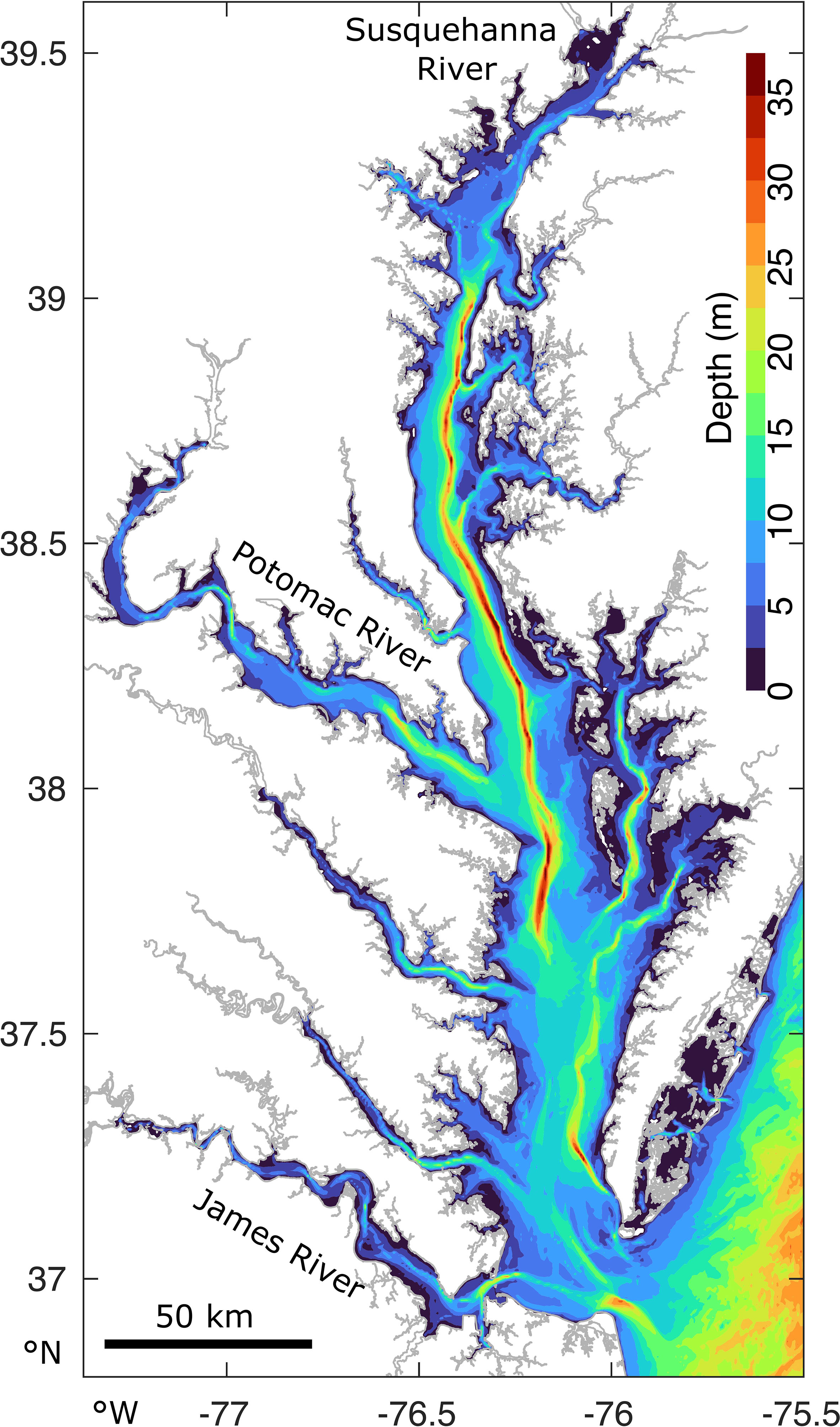
Figure 1 The Chesapeake Bay and its bathymetry and main tributaries, located on the East Coast of the U.S.A.

The Chesapeake Bay has been systematically sampled within the Chesapeake Bay Program, resulting in long-term, biweekly or monthly, in situ collection of a variety of physical and biogeochemical variables (Table 1). For a detailed description of the methodology, we refer the reader to Chesapeake Bay Program (2022). We start from P. minimum cell counts at 37 stations in the Chesapeake Bay (Figure 2) and extract the corresponding nineteen physical and biogeochemical variables based on station and date. This activity results in a data set consisting of 3609 observations of P. minimum cell counts and corresponding variables of interest. The number of blooms is 256. Most observations were collected in the main channel and the majority of blooms occurred in the upper region of the Chesapeake Bay (Figure 2A) in April-May (Figure 2B).

TABLE 1

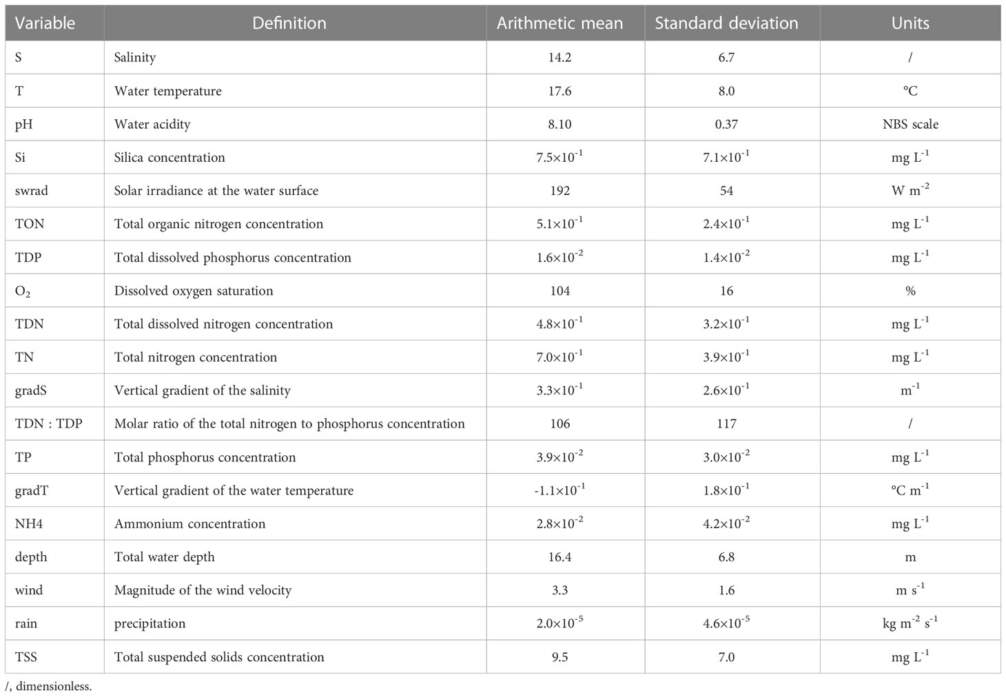
Table 1 The nineteen environmental variables used to train the P. minimum models and their mean and standard deviation observed at the surface (< 1 m) in the Chesapeake Bay between 1984-2020.

FIGURE 2

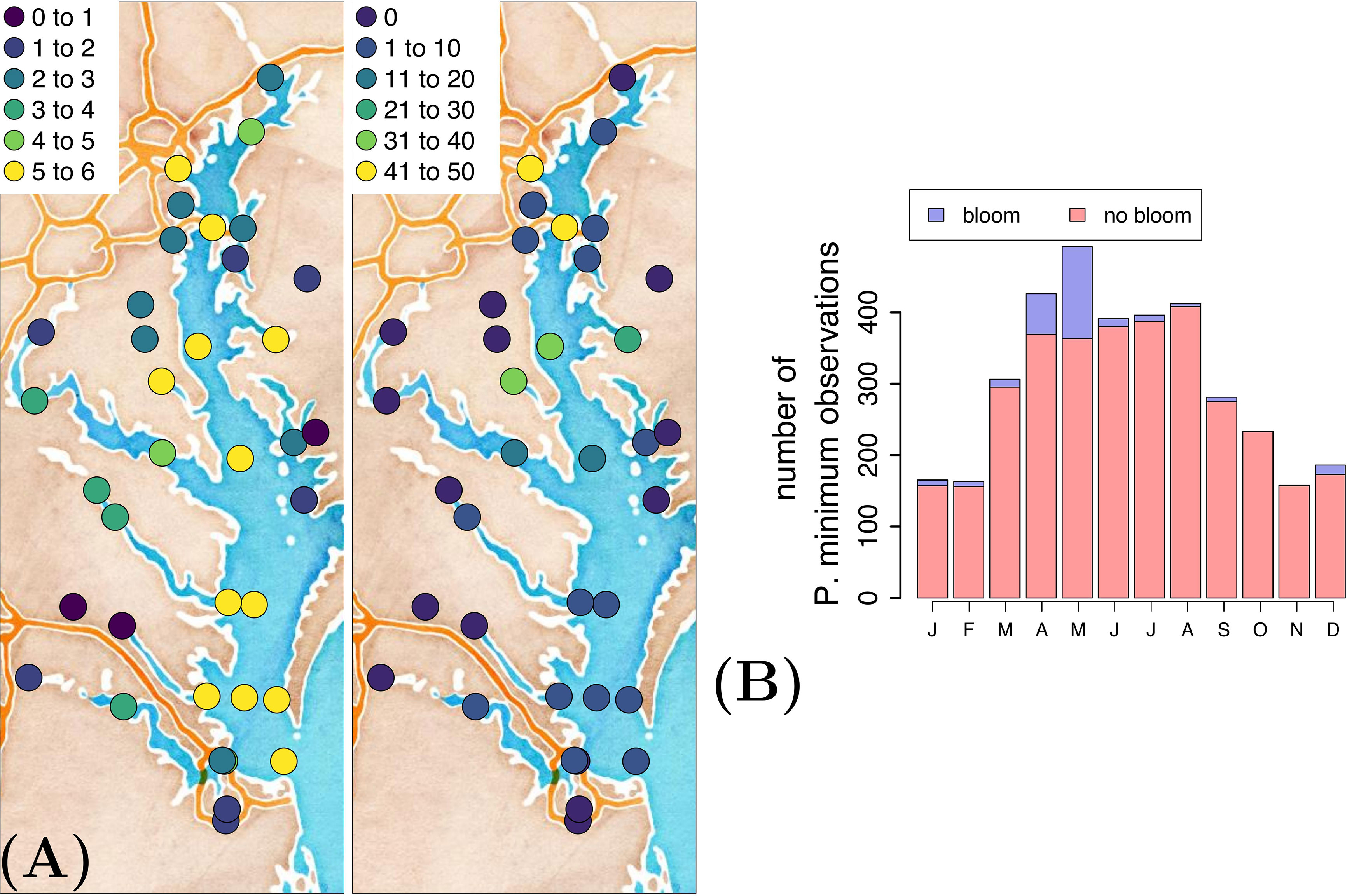
Figure 2 (A) Natural logarithmic number of P. minimum observations (left) and number of P. minimum blooms (right), and (B) temporal distribution of the P. minimum observations at 37 stations in surface waters (i.e.,<1 m water depth).

We only use observations in the surface waters (i.e., < 1 m water depth), with the exception of the vertical gradient of salinity and water temperature. The reason is that P. minimum cell counts at deeper water depth are unavailable. Solar irradiance, wind, and rain are from the ERA5 reanalysis (Hersbach et al., 2020), which provides hourly estimates on a 1/4 deg. grid. Long-term daily-averaged values of solar irradiance are computed so they solely depends on Julian day (cf., no spatial variability and a reduction of temporal variability caused by, for example, clouds). Water depth is estimated using long-term time-averages of observations collected between 1984-2020, resulting in a fixed water depth at each station (cf., no temporal variability). Because we are interested in biological activity (cf., blooms), we estimate the dissolved oxygen saturation from salinity, temperature, atmospheric pressure, and dissolved oxygen observations (Dataset U.S. Geological Survey, 2011). The vertical gradients in salinity and temperature are calculated from the slope of a linear fit that we apply to the salinity and temperature observations over depth, requiring that at least 50% of the total water depth was sampled.

2.2 Statistical models

In this section, we briefly introduce the binomial distribution, and the two statistical models that we apply: GLMs and GAMs.

2.2.1 The binomial distribution

Before presenting the GLM and GAM, we introduce some concepts of the binomial distribution that are required to understand the core assumptions made to construct these models: probability p, the expected value µ, and link or logit function g.

Our bloom data are binary: a bloom occurs or it does not. Therefore, we assume that the bloom data follows a Bernoulli distribution or, because multiple Bernoulli trials are considered, a binomial distribution. The probability mass function of the latter distribution in 1D reads as

$\begin{array}{ll}f(y;n,p)=\left(\begin{array}{c}n\\ y\end{array}\right)p^y(1-p{)}^{n-y},& (1)\end{array}$

in which n is the total number of trials, p is the probability of a bloom, y ∈ {0, 1, ..., n} is the number of successes (i.e., blooms), and $\left(\genfrac{}{}{0ex}{}{n}{y}\right)$ = n!/[k!(n − k)!] is the binomial coefficient. We can write Eq. (1) in its exponential form by applying the identity operator exp[ln()]:

$\begin{array}{ll}f\left(y;n,p\right)=\left(\begin{array}{c}n\\ y\end{array}\right)\text{exp\hspace{0.17em}}[\eta y-\underset{\begin{array}{c}|\\ \hfill \hspace{1em}\to \text{A}(\eta ;n)\end{array}}{\underbrace{nln(1+e^{\eta })\text{],}}}& (2)\end{array}$

with

$\begin{array}{ll}\eta =\ln \frac{p}{1-p}.& (3)\end{array}$

The expected value E[y;η,p] is defined as

$\begin{array}{ll}\mu =E[y;n,p]=\sum _{y=0}^{n}yf(y;n,p)& (4)\end{array}$

Summation of Eq. (2) from y = 0 to η, taking the derivative of both side to η, and using the normalization property $\sum _{y=0}^{n}f(y;n,p)=1$, it can be shown that

$\begin{array}{ll}\mu ={\partial }_{\eta }A(\eta ;n)=g^{-1}(\eta )=n\frac{e^{\eta }}{1+e^{\eta }},& (5)\end{array}$

where g is the link function, that is, linking µ to η, which reads as

$\begin{array}{ll}g=\ln \frac{\mu }{n-\mu }.& (6)\end{array}$

The latter function is also known as the logit or log-odds function.

2.2.2 Generalized linear models

A GLM assumes that η can be expressed as a linear combination of the environmental variable x_i (e.g., salinity, temperature). Following the same reasoning, if we have k independent environmental variables, a GLM assumes

$\begin{array}{ll}\eta ={\beta }_0+\sum _{i=1}^k{\beta }_i{x}_i& (7)\end{array}$

The variables x₁,…x_k are normalized to balance the order of magnitude of the various terms in Eq. (7):

$\begin{array}{ll}{x}_i=\frac{{\tilde{x}}_i-\text{mean}(x_i)}{\text{std}(x_i)},& (8)\end{array}$

in which ${\tilde{x}}_i$ is the dimensional observation of x_i, and mean(x_i) and std(x_i) are the arithmetic mean and standard deviation of all considered (dimensional) observations of x_i, respectively. The normalization enables a fair comparison of the response of varying various environmental variables [cf., terms in Eq. (7)] and the probability of a bloom. By maximizing the likelihood function ℒ(p;n,y), that is, given n and y, what is the most realistic estimate of p [cf., swap the conditional of f(y;n,p)], we determine the fitting parameters β₀,…β_k. The transformation between p, η (and thus β₀,…β_k) follows from Eq. (3):

$\begin{array}{ll}p=\frac{1}{1+e^{-\eta }}.& (9)\end{array}$

Once we estimated β₀,…β_k, we can thus compute a probability of a bloom p using this equation given x₁,…x_k.

2.2.3 Generalized additive models

GAMs are an extension of GLMs in which we allow for nonlinear (interaction) terms:

$\begin{array}{ll}\eta ={\beta }_0+\sum _{i=1}^k{s}_i(x_i)+\underset{\text{interaction\hspace{0.17em}terms}}{\underbrace{{\displaystyle \sum _{i=1}^{k-1}{\displaystyle \sum _{j=i+1}^k{\text{S}}_{ij}(x_i{x}_j)}}}},& (10)\end{array}$

where the coefficients β_i are replaced by nonlinear functions s_i and s_ij. In addition to its nonlinear characteristics, this approach allows us to consider the effect of interactions. For example, what is the effect of the interaction of salinity and temperature on the probability of a bloom to occur. To fit the functions s_i and s_ij to the in situ data, we again maximize the likelihood functions ℒ. To avoid overfitting, which results in a less generic model, we add a penalty term that quantifies the degree of ‘quivering’ of the fitted curve by taking the square of the second derivative (the second derivative quantifies how fast the gradient changes and is thus a measure for its short-term change). We use the thin plate spline approach, which constructs s_ij (x_i,x_j) [or s_i(x_i)] using radial basis functions [i.e., ϕ(r) = r² ln (r)] and has a penalty term:

$\begin{array}{ll}-{\lambda }_{ij}{\int }^{}{\int }^{}\left\{[{\partial }_{x_i{x}_i}{s}_{ij}(x_i,x_j){]}^2+2[{\partial }_{x_i{x}_j}{s}_{ij}(x_i,x_j){]}^2+{[{\partial }_{x_j{x}_j}{s}_{ij}(x_i,x_j)]}^2\right\}d{x}_{i}d{x}_j,& (11)\end{array}$

in which λ_ij is a scaling factor to control the weight of the penalty term. For the technical details and implementation, we refer the reader to Dobson and Barnett (2018), Wood (2006), and the functions glm() and gam() of the stats and mgcv packages provided by the open-source R statistical software.

2.2.4 Imbalanced data

The P. minimum bloom data are heavily skewed, that is, the number of observed blooms is significantly fewer than the number of no-bloom occurrences (ratio<10%). This imbalance hinders the construction of a useful model (Chawla et al., 2004; Kim et al., 2021). A model constructed with such a distribution would generally forecast a no-bloom event with an overall high accuracy >90%, simply due to the low percentage of observed blooms. To avoid this outcome, we apply the Synthetic Minority Over-sampling Technique e (SMOTE) (Chawla et al., 2011). This method increases the number of bloom data points by generating synthetic data of a suite of physical-biogeochemical predictors associated with observed blooms. A synthetic bloom data point (which is represented by a value 1) is created by (1) randomly selecting one out of five nearest neighboring bloom data points of a real bloom data point in the multidimensional (cf., number of variables under consideration) variable-vector space, (2) subtracting the selected nearest neighbor and the bloom data vector of focus, (3) multiplying this difference by a random number between 0.25 and 0.75, and (4) adding this scaled difference to the bloom data point under consideration. Synthetic data points are only used to train the model. To estimate model accuracy, only real observations are used as test data.

2.2.5 Goodness-of-fit and optimal variable combination

We computed the goodness-of-fit of the statistical models using three quantities: the AIC, the accuracy of forecasting a bloom α₁, and the accuracy of a no-bloom occurrence α₀:

$\begin{array}{ll}\text{AIC}=2k^{\prime }-2\ln (ℒ),& (12)\end{array}$

$\begin{array}{ll}{\alpha }_1=\frac{N_1^{pred}}{N_1^{obs}},& (13)\end{array}$

$\begin{array}{ll}{\alpha }_0=\frac{N_0^{pred}}{N_0^{pred}},& (14)\end{array}$

in which k’ is the number of model parameters, ℒ is the likelihood function of the model, $N_1^{obs}$ and $N_0^{obs}$ are the observed, and $N_1^{pred}$ and $N_0^{pred}$ are the correctly forecasted number of bloom and no-bloom events, respectively. From Eq. (12), we see that a lower AIC value corresponds to a better goodness-of-fit; the number of model parameters increases the AIC, whereas a higher likelihood decreases this quantity. From Eqs. (13)-(14), the total model accuracy α is

$\begin{array}{ll}\alpha =\frac{N_1^{obs}{\alpha }_1+N_0^{obs}{\alpha }_0}{N_1^{obs}+N_0^{obs}}& (15)\end{array}$

To avoid overfitting the GLM, an optimal combination of up to five environmental variables were identified based on the AIC (Figure S1, Supplementary Material). This can also be derived by the following simple reasoning: if we require a minimum of five observations for each dimension (cf., environmental variable), the number of variables D is limited by the total number of data points to train the model ~ 3000, that is, 5^D ~ 3000, or D~ 5. Using up to five variables, the total number of variable combinations C is

$\begin{array}{ll}\mathcal{C}=\sum _{D=1}^5\frac{N^{var}!}{D!(N^{var}-D)!}=16663& (16)\end{array}$

in which N^var = 19 is the total number of variables to choose from. For each variable combination, we train 50 GLMs to incorporate the variability that is related to the random subdivision of the data into a training and test data set required to construct a GLM. We thus train a total of 50×16663>800,000 GLMs. We compute the averaged (of the 50 GLMs) AIC and accuracy α₁ and α₂, and estimate the uncertainty by computing the standard deviation. The optimal variable combinations are determined by requiring that the corresponding AIC is <7.5 percentile, and model accuracy α>92.5 percentile, that is, selecting the ~ 7.5% best results. To quantify the potential of applying individual variables to forecast P. minimum blooms, we compute the probability that a variable is present in this set of optimal variable combinations (‘Probability selected’) and its ‘Correlation to a bloom’, which varies between -1 (variable is always negatively associated with the probability of a bloom) and 1 (variable is always positively associated with the probability of a bloom).

3 Results

3.1 Generalized linear models

Of the nineteen variables examined, S, T, and pH were found to be the optimal predictors in forecasting a P. minimum bloom (Table 2; Probability selected >50%). S and T are always negatively associated with a bloom, whereas pH is linked to an increase of the probability of a bloom to occur (Table 2). The second most important predictors (Probability selected >20%) are nutrients Si, TON, and TDP, and swrad. Si and TDP are linked to a decrease of the probability of a bloom to occur, whereas swrad and TON are linked to an increase. All other variables have a probability less than 20%. The goodness-of-fit of all 16,663 variable combinations and the corresponding set of optimal combinations that was used to determine the Probability selected and Correlation to a bloom can be found in the Supplementary Material (Figure S1).

TABLE 2

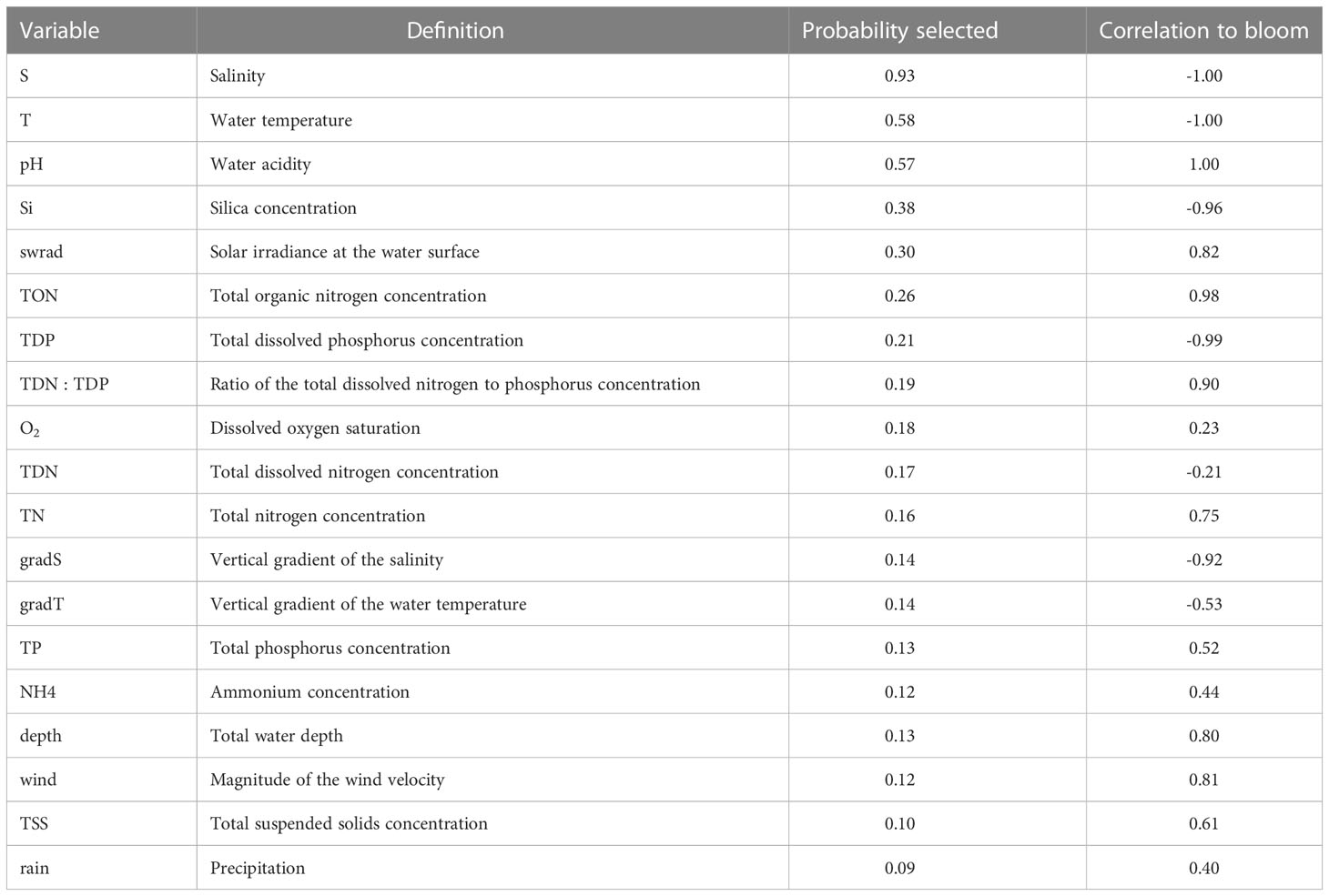
Table 2 Ranking the nineteen variables based on their effectiveness in forecasting P. minimum blooms (cf., Probability selected) and the corresponding effect on these blooms (cf., Correlation to bloom) using a generalized linear model.

Based on the AIC, the optimal five-variable combination is {T, S, pH, swrad, TON} (Table 3). If we only include three and four variables to train the GLM, the optimal sets are {T, S, pH} and {T, S, pH, swrad}, respectively. Including four or five variables results in a significantly better model based on the AIC compared to using only three variables (Welch two-tailed t-test, both p-values<2.2×10^-16). Considering five instead of four variables also results in a significantly better AIC (Welch two-tailed t-test, p-value =1.8×10^-12). Because pH, O₂, and nutrients may be linked to a consequence of a bloom rather than a cause, we also determine the optimal set when we exclude these variables. This results in optimal variable combinations {T, S, swrad}, {T, S, swrad, depth}, and {T, S, swrad, depth, wind} when restricting the number of variables to three, four, and five, respectively. Based on the AIC, the model is significantly better when using all five variables instead of only three (Welch two-tailed t-test, p-value =1.9×10^-6) or four (Welch two-tailed t-test, p-value = 2.6×10^-2). The model also significantly improves when including four instead of three variables (Welch two-tailed t-test, p-value =8.5×10^-3).

TABLE 3

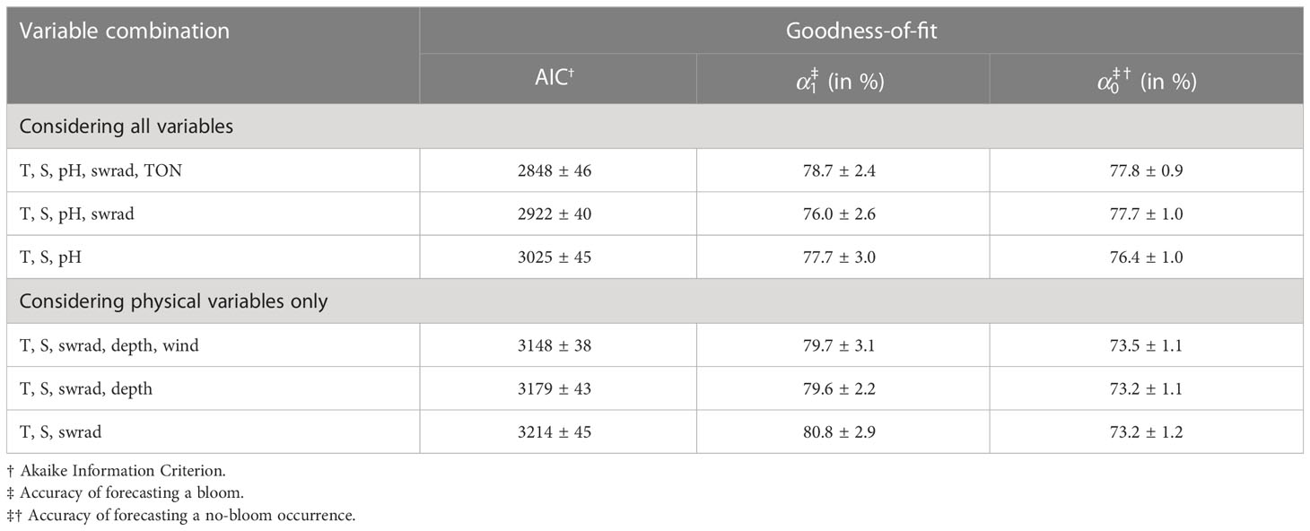
Table 3 Optimal variable combination with and without consideration of biogeochemical environmental variables to train the generalized linear model and the corresponding goodness-of-fit.

Model accuracy of forecasting a bloom and no-bloom occurrence varies in both space and time for the optimal variable combination {T, S, pH, swrad, TON} (Figure 3). The GLM forecasts blooms more accurately in the upper Bay region and tends to not forecast them well in its lower reaches (Figure 3A). Conversely, in the lower portion of the Bay, the model more accurately forecasts no-bloom events. From a seasonal perspective, the GLM forecasts P. minimum blooms relatively accurately in spring (March-June), yet is less accurate in forecasting no-bloom events during this time period (Figure 3B). The opposite is true in all other seasons.

FIGURE 3

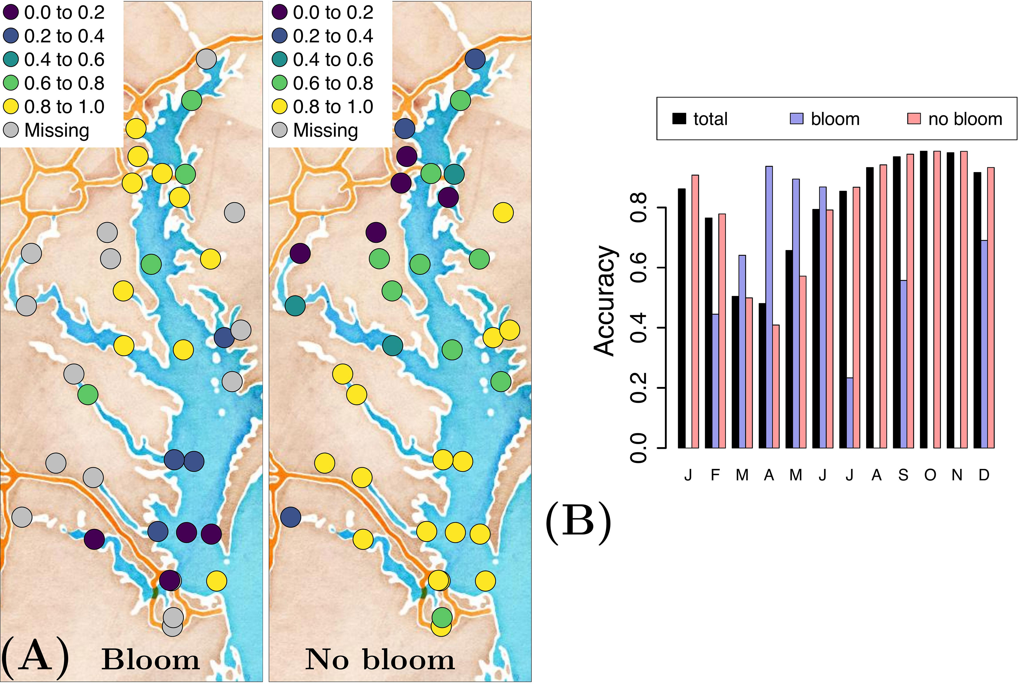
Figure 3 (A) Accuracy of forecasting a P. minimum bloom and no-bloom occurrence, and (B) the corresponding temporal distribution of the accuracy when using the optimal variable combination {T, S, pH, swrad, TON} and applying a generalized linear model.

3.2 Generalized additive models

To better understand the temporal and spatial variability in the accuracy of forecasting P. minimum blooms and increase overall model performance, we also applied GAMs to account for nonlinear effects (Table 4). We only consider the two extremes: the optimal variable combination {T, S, pH, swrad, TON}, and the three-variable optimal model in which we only include physical variables {T, S, swrad}. The optimal five-variable combination yields a significantly greater model performance based on the AIC (Welch two-tailed t-test, p-value =6.8×10^-6) than the three-variable optimal model (Table 4). In addition, GAMs that consider interactive terms are significantly better compared to GAMs that do not include these terms (Welch two-tailed t-test, p-value =8.6×10^-11 and =5.3×10^-12, respectively). Interestingly, the model constructed using T, S, and swrad that includes interactions improves model performance more than the model using all five variables {T, S, pH, swrad, TON} without interactions (Welch two-tailed t-test, p-value =3.8×10^-9).

TABLE 4

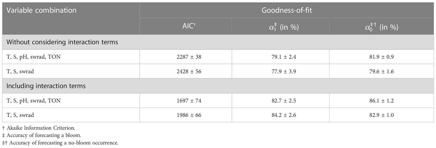
Table 4 Goodness-of-fit corresponding to the generalized additive model with and without consideration of interaction terms.

Inclusion of the interaction terms clearly improves model performance when we analyze the temporal and spatial variability of the model accuracy. For example, when we compare the accuracy with and without interactions (Figures 4A, B), we see more points with model accuracy > 0.6 (green and yellow) in the case with interactions, and more points with lower accuracy (dark blue) in the case without interactions. A similar pattern is seen for the temporal variability of the accuracy (Figures 4C, D); inclusion of interaction terms uniformizes the accuracy of forecasting a bloom in time (less variability in the size of the blue bars). To summarize, the model continues to better forecast the blooms located in the upper region of the Bay and no-bloom events in its southern portion, yet model accuracy is more uniform in both space and time when interaction terms are included in the model.

FIGURE 4

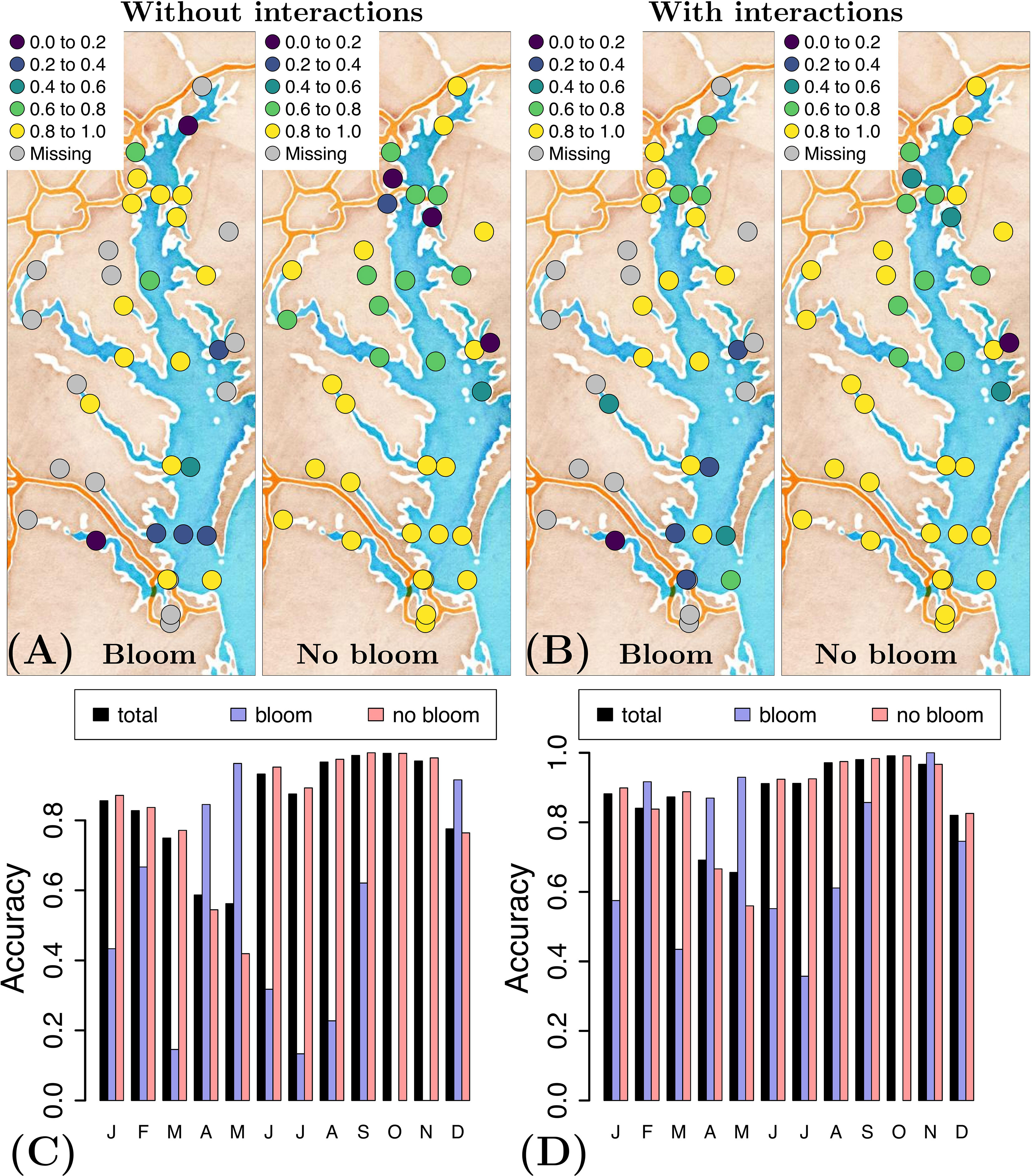
Figure 4 Accuracy of forecasting a P. minimum bloom and no-bloom (A) without and (B) with consideration of interactions, and the corresponding temporal distribution of the accuracy (C) without and (D)with consideration of interactions, using the optimal variable combination {T, S, pH, swrad, TON} and applying a generalized additive model.

3.3 The effect of nonlinearities on bloom probability

Including nonlinear effects in the GAM allows the model to have a range of environmental conditions in which the probability of a P. minimum bloom is optimized. This corresponds to a (nonlinear) local maximum in η -x_i space, which is not possible in a GLM. The nonlinear response of the probability of a bloom to S (s_s) and T (s_T) indeed shows such a local maximum at a specific range of S and T [(Figures 5A, B); horizontal red arrows] centered at ~ 8 and ~ 15°C, respectively. The dots and shaded area depict the partial residuals and two standard error bounds, respectively.

FIGURE 5

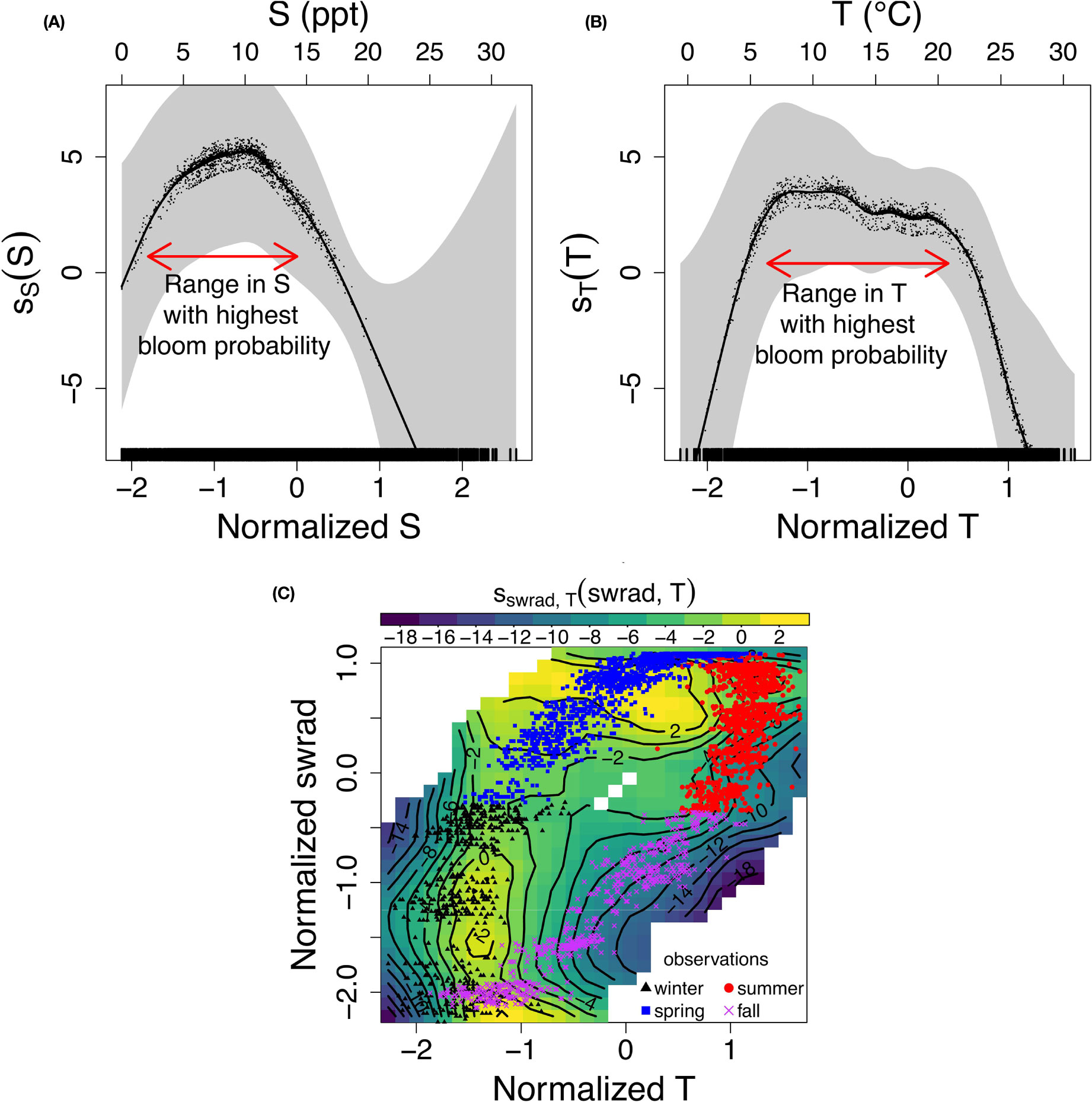
Figure 5 (A–C) Nonlinear response of (the logit of) the probability of a P. minimum bloom to (normalized) (A) salinity (S), (B) water temperature (T), and (C) interacting (normalized) T and solar irradiance (swrad), and the corresponding observations assuming a generalized additive model with interaction terms [Eq. (10)] and the optimal variable combination {T, S, pH, swrad, TON}.

The nonlinear interaction of terms captures the seasonal pattern of the probability of bloom occurrence, and result in an increase of goodness-of-fit and more consistent model accuracy over time. Specifically, the swrad-T interaction term partly captures the seasonality of bloom occurrence, that is, only a few blooms were observed in fall and most blooms occur in spring (Figure 5C). Indeed, the model forecasts a decrease in the probability of a bloom (blue/green region, contour <-6) corresponding to the fall observations and an increase (yellow region, contour > 2) corresponding to spring observations. For completeness, we added the GAM response to all other (interacting) variables to the Supplementary Material (Figures S2–S4).

4 Discussion

4.1 Importance of biogeochemistry and hydrodynamics

By training statistical models using more than 16,000 variable combinations of nineteen physical and biogeochemical variables, we showed that salinity, water temperature, pH, total organic nitrogen (TON), and solar irradiance is the optimal variable combination to forecast P. minimum blooms in the Chesapeake Bay. Our analysis also allowed us to determine the effectiveness of individual environmental variables in forecasting P. minimum blooms (Table 2) and the corresponding effect on these bloom forecasts. Salinity, temperature, and to a lesser extent, solar irradiance are the most important variables that affect the probability of a bloom. In addition to these physical factors, pH, silica, organic nitrogen, and dissolved phosphorus play a role in forecasting these blooms. Organic nitrogen and pH show a strong positive correlation to the presence of P. minimum blooms, whereas silica and dissolved phosphorus are negatively correlated to these blooms. These findings are consistent with various studies presented in the literature. Hansen (2002) showed that P. minimum tolerates relatively high pH values (> 9) compared to two other dinoflagellate taxa (i.e., Ceratium lineatum and Heterocapsa triquetra) in laboratory experiments, and that growth rate reaches a maximum at a pH of ∼ 8. Olenina et al. (2010) found a correlation between P. minimum abundance and pH in the coastal region of Lithuania. The negative relationship of bloom probability with silica may be due to competition with diatom taxa, which require silica, while P. minimum does not. For example, the diatom Skeletonema costatum is often dominant in the Chesapeake Bay (Marshall et al., 2006). The positive response of a bloom to organic nitrogen agrees with Glibert et al. (2001) who found that P. minimum blooms in spring in 1998 typically occurred after a peak of urea. Finally, the negative relationship with dissolved phosphorus complies with Li et al. (2015) who showed that P. minimum blooms are associated with low phosphate concentrations in the Chesapeake Bay. Bi et al. (2021) also found a negative relationship between the ratio of particulate organic nitrogen to particulate organic phosphorus and diatom to P. minimum ratio.

4.2 Nonlinear dependence

Adding nonlinear (interacting) dependencies between predictor variables results in valuable insights into the impact of these dependencies on the probability of a P. minimum bloom occurring, and may explain the improvement in the model’s ability to forecast blooms. The nonlinear local maximum of the model response of the probability of a bloom to salinity and temperature, centered at ~ 8 and ~ 15°C, respectively (Figures 5A, B), suggests that a high probability of a bloom is constrained to specific regions of the Chesapeake Bay. This restriction reduces error attributable to spatial variability (Figure 3A versus Figure 4A). In addition, the model stresses the importance of the nonlinear seasonal interaction between solar irradiance and temperature, which is likely caused by the delayed effect of water cooling and warming due to thermal inertia (Figure 5C). This seasonal interaction between solar irradiance and water temperature partly captures the seasonal hysteresis pattern observed in this interaction, which may explain the further increase of the goodness-of-fit (i.e., decrease in AIC) and uniformity of the model accuracy in time (Figures 4C, D). These results highlighting the need for nonlinearities comply with previous studies. Tango et al. (2005) found that P. minimum mainly blooms in April-May in the upstream region of the Bay and showed that the blooms were restricted to salinities of 4.5-12.8 and water temperatures of 12-28°C. This was confirmed by Li et al. (2015) who demonstrated that the optimal temperature and salinity ranges are 5-10 and 15-20°C. respectively. Fan and Glibert (2005) indicated that urea uptake, which is most closely related to TON in our set of five optimal variables, increased with increasing solar irradiance during a bloom in the Choptank River, thus showing the importance of the TON-solar irradiance interaction.

4.3 Model limitations and assumptions

Several assumptions and limitations are imposed to construct our habitat suitability models, which may impact model performance and its application. Though we compared P. minimum cell counts and environmental factors measured on the same date near the water surface, we assume that the response of a bloom and a set of environmental conditions is instantaneous (i.e., within one day) and vertical processes are of little importance. However, we know that P. minimum needs time to grow and has various life cycle stages (cf., cyst stage), with typical time scales on the order of multiple days (Heil et al., 2005). In addition, P. minimum may show a vertical gradient caused by both active (i.e., vertical migration; Olsson and Granéli, 1991) and passive (i.e., water flow; Li et al., 2021) processes.

The relatively small number of coincident observations of P. minimum cell counts and environmental variables, as well as the limited number of P. minimum blooms compared to the number of total observations in the data set used in training, testing, and validating the models, imposes limitations that must, if possible, be remedied. In regards to the skewed number of blooms in the data set, we applied the SMOTE method to generate synthetic bloom data points to balance the bloom/no-bloom observations. To employ the largest data set possible, we used a data set covering ∼ 35 years and thus assume that the response of a bloom to environmental conditions and the sampling methodology are fixed over these years. However, we know that, for example, detection limits for various variables have been lowered over these years [for changes in methodology, see Chesapeake Bay Program (2022)]. Based on an analysis of the frequency distribution of the in situ observations, we do not expect a major impact of changes in the detection limits on our model application (for more details, we refer the reader to the Supplementary Material; Figures S5–S8). Furthermore, we assume a stationary response of P. minimum to the environment. These assumptions may all affect the model performance. We therefore stress the importance of additional observations and continued monitoring campaigns to augment the essential data sets used in this analysis. Future observations of P. minimum blooms and corresponding environmental variables that are known to affect these blooms are required to further improve our results and test their sensitivity to our assumptions.

5 Summary and conclusions

Forecasts of harmful algal blooms (HABs) are highly desired by stakeholders, such as coastal managers and aquaculturists, so they are able to assess risks associated with the presence of HABs and respond accordingly. With this in mind, our objective is to add HABs into our suite of forecasts available through the Chesapeake Bay Environmental Forecasting System (CBEFS) (www.vims.edu/cbefs; Bever et al., 2021). Here, we constructed empirical habitat suitability models with and without consideration of nonlinearities to forecast the P. minimum blooms in the Chesapeake Bay using a set of environmental factors for which decades of in situ observations exist. By training statistical models using more than 16,000 combinations of nineteen environmental variables and comparing goodness-of-fit, we showed that using a small subset of these variables provides optimal results. Specifically, salinity, water temperature, pH, total organic nitrogen, and solar irradiance form the optimal set of variables required to forecast a P. minimum bloom. Including nonlinear interactions between these variables improves the model’s ability to forecast the blooms (increase in accuracy of ~ 10%) and provides valuable insights into the variability of the model’s ability to spatially and temporally forecast these blooms. For example, a nonlinear response between the probability of a bloom and (interacting) environmental conditions showed high probability of blooms in specific regions (cf., range of salinity) and seasons (cf., range of temperature and interaction between solar irradiance and temperature). Given the dynamical complexities of P. minimum blooms, we found surprisingly high overall model accuracy (up to ∼ 85%). Our study highlights that additional observations of P. minimum blooms and corresponding environmental variables that are known to affect these blooms would be required to diminish model limitations and increase model accuracy (at all times). One of the key findings of our study is that this accuracy may vary based on the region and season of interest. To our knowledge, this is the first instance in which a study has provided seasonally and spatially dependent model accuracies for HAB occurrence. Before our work, neither a qualitative nor quantitative picture of this variability was available. Insight into the variability in model accuracy in time and space is crucial for users of forecasts derived from this model. Knowing the regions and season that come with lower model forecasting accuracy can guide monitoring program managers when and where to collect in situ observations so they can optimize limited available funding and partly resolve these knowledge gaps. This will likely increase model accuracy (at all times). Even with these existing accuracy levels, we have found that coastal resource managers are already using our forecasts to visit locations where the likelihood of finding a bloom is highest. Stakeholders focus group meetings with anglers have also revealed that anglers and charter boat captains will use these forecasts to help them decide when and where to fish, so they have the greatest chance of avoiding direct contact with HABs. Finally, apart from their forecasting potential, our findings may be particularly useful to construct explicit relationships between environmental variables and P. minimum presence in mechanistic models. Ultimately, these insights will be used to extend CBEFS with forecasts of P. minimum blooms by forcing our empirical habitat suitability model using modeled forecasts of salinity, water temperature, pH, total organic nitrogen, and solar irradiance instead of in situ observations.

Data availability statement

Publicly available datasets were analyzed in this study. This data can be found here: https://www.chesapeakebay.net/what/data.

Author contributions

DH: Conceptualization, Formal analysis, Investigation, Methodology, Software, Validation, Visualization, Writing: original draft preparation, review and editing, Data curation. MF: Conceptualization, Investigation, Writing: review and editing. PS-L: Conceptualization, Investigation, Resources, Writing: review and editing. RH: Conceptualization, Investigation, Writing: review and editing. CB: Conceptualization, Investigation, Writing: review and editing. All authors contributed to the article and approved the submitted version.

Funding

This paper is the result of research funded by the National Oceanic and Atmospheric Coastal Ocean and Modeling Testbed Project under award NA21NOS0120167 to VIMS. Chris Brown was supported by the NOAA Center for Satellite Applications and Research.

Acknowledgments

The authors acknowledge William & Mary Research Computing (https://www.wm.edu/it/rc) for providing computational resources and/or technical support that have contributed to the results reported within this paper. The scientific results and conclusions, as well as any views or opinions herein, are those of the authors and do not necessarily reflect those of NOAA or the Department of Commerce.

Conflict of interest

The authors declare that the research was conducted in the absence of any commercial or financial relationships that could be construed as a potential conflict of interest.

Publisher’s note

All claims expressed in this article are solely those of the authors and do not necessarily represent those of their affiliated organizations, or those of the publisher, the editors and the reviewers. Any product that may be evaluated in this article, or claim that may be made by its manufacturer, is not guaranteed or endorsed by the publisher.

Supplementary material

The Supplementary Material for this article can be found online at: https://www.frontiersin.org/articles/10.3389/fmars.2023.1127649/full#supplementary-material

References

Akaike H. (1998). “Information theory and an extension of the maximum likelihood principle,” in Selected papers of Hirotugu Akaike (Springer), 199–213. doi: 10.1007/978-1-4612-1694-0_15

CrossRef Full Text | Google Scholar

Anderson C. R., Moore S. K., Tomlinson M. C., Silke J., Cusack C. K. (2015). Living with harmful algal blooms in a changing world: Strategies for modeling and mitigating their effects in coastal marine ecosystems. Coast. Mar. Hazards Risks Disasters, 495–561. doi: 10.1016/B978-0-12-396483-0.00017-0

CrossRef Full Text | Google Scholar

Anderson C. R., Sapiano M. R., Prasad M. B. K., Long W., Tango P. J., Brown C. W., et al. (2010). Predicting potentially toxigenic Pseudo-nitzschia blooms in the Chesapeake Bay. J. Mar. Syst. 83, 127–140. doi: 10.1016/J.JMARSYS.2010.04.003

CrossRef Full Text | Google Scholar

Bever A. J., Friedrichs M. A., Friedrichs C. T., Scully M. E., Lanerolle L. W. (2013). Combining observations and numerical model results to improve estimates of hypoxic volume within the Chesapeake Bay, USA. J. Geophysical Res.: Oceans 118, 4924–4944. doi: 10.1002/JGRC.20331

CrossRef Full Text | Google Scholar

Bever A. J., Friedrichs M. A., St-Laurent P. (2021). Real-time environmental forecasts of the Chesapeake Bay: Model setup, improvements, and online visualization. Environ. Model. Softw. 140, 105036. doi: 10.1016/J.ENVSOFT.2021.105036

CrossRef Full Text | Google Scholar

Bi R., Cao Z., Ismar-Rebitz S. M., Sommer U., Zhang H., Ding Y., et al. (2021). Responses of marine diatom-dinoflagellate competition to multiple environmental drivers: Abundance, elemental, and biochemical aspects. Front. Microbiol. 12. doi: 10.3389/FMICB.2021.731786/BIBTEX

PubMed Abstract | CrossRef Full Text | Google Scholar

Brown C. W., Hood R. R., Long W., Jacobs J., Ramers D. L., Wazniak C., et al. (2013). Ecological forecasting in Chesapeake Bay: Using a mechanistic-empirical modeling approach. J. Mar. Syst. 125, 113–125. doi: 10.1016/j.jmarsys.2012.12.007

CrossRef Full Text | Google Scholar

Carstensen J., Klais R., Cloern J. E. (2015). Phytoplankton blooms in estuarine and coastal waters: Seasonal patterns and key species. Estuarine Coast. Shelf Sci. 162, 98–109. doi: 10.1016/J.ECSS.2015.05.005

CrossRef Full Text | Google Scholar

Chawla N. V., Bowyer K. W., Hall L. O., Kegelmeyer W. P. (2011). SMOTE: Synthetic minority over-sampling technique. J. Artif. Intell. Res. 16, 321–357. doi: 10.1613/jair.953

CrossRef Full Text | Google Scholar

Chawla N. V., Japkowicz N., Kotcz A. (2004). Special issue on learning from imbalanced data sets. ACM SIGKDD Explor. Newslett. 6, 1–6. doi: 10.1145/1007730.1007733

CrossRef Full Text | Google Scholar

Cruz R. C., Costa P. R., Vinga S., Krippahl L., Lopes M. B. (2021). A review of recent machine learning advances for forecasting harmful algal blooms and shellfish contamination. J. Mar. Sci. Eng. 9 (3), 283. doi: 10.3390/JMSE9030283

CrossRef Full Text | Google Scholar

Dataset Chesapeake Bay Program (2022) Chesapeake Bay Program data. Available at: https://www.chesapeakebay.net/what/data (Accessed 2022-09-12).

Google Scholar

Dataset U.S. Geological Survey (2011) . change to solubility equations for oxygen in water: Office of water quality technical memorandum 2011.03. Available at: https://water.usgs.gov/water-resources/memos/documents/WQ.2011.03.pdf.

Google Scholar

Díaz P. A., Ruiz-Villarreal M., Pazos Y., Moita T., Reguera B. (2016). Climate variability and Dinophysis acuta blooms in an upwelling system. Harmful Algae 53, 145–159. doi: 10.1016/J.HAL.2015.11.007

PubMed Abstract | CrossRef Full Text | Google Scholar

Ding J., Tarokh V., Yang Y. (2018). Model selection techniques: An overview. IEEE Signal Process. Magazine 35, 16–34. doi: 10.1109/MSP.2018.2867638

CrossRef Full Text | Google Scholar

Dobson A. J., Barnett A. G. (2018). An introduction to generalized linear models (Chapman and Hall/CRC).

Google Scholar

Fan C., Glibert P. M. (2005). Effects of light on nitrogen and carbon uptake during a Prorocentrum minimum bloom. Harmful Algae 4, 629–641. doi: 10.1016/J.HAL.2004.08.012

CrossRef Full Text | Google Scholar

Flynn K. J., McGillicuddy D. J. (2018). Modeling marine harmful algal blooms: Current status and future prospects. Harmful Algal. Blooms, 115–134. doi: 10.1002/9781118994672.CH3

CrossRef Full Text | Google Scholar

Frankel L. T., Friedrichs M. A., St-Laurent P., Bever A. J., Lipcius R. N., Bhatt G., et al. (2022). Nitrogen reductions have decreased hypoxia in the Chesapeake Bay: Evidence from empirical and numerical modeling. Sci. Total Environ. 814, 152722. doi: 10.1016/j.scitotenv.2021.152722

PubMed Abstract | CrossRef Full Text | Google Scholar

Franks P. J. S. (2018). Recent advances in modelling of harmful algal blooms. In: Glibert P., Berdalet E., Burford M., Pitcher G., Zhou M. (eds) Global Ecol. Oceanography Harmful Algal Blooms (Springer, Cham: Ecological Studies), 232. doi: 10.1007/978-3-319-70069-4_19

CrossRef Full Text | Google Scholar

Gallegos C. L., Bergstrom P. W. (2005). Effects of a prorocentrum minimum bloom on light availability for and potential impacts on submersed aquatic vegetation in upper Chesapeake Bay. Harmful Algae 4, 553–574. doi: 10.1016/J.HAL.2004.08.016

CrossRef Full Text | Google Scholar

Gallegos C. L., Jordan T. E. (2002). Impact of the spring 2000 phytoplankton bloom in Chesapeake Bay on optical properties and light penetration in the Rhode River, Maryland. Estuaries 4(25), 508–518. doi: 10.1007/BF02804886

CrossRef Full Text | Google Scholar

Glibert P. M., Berdalet E., Burford M. A., Pitcher G. C., Zhou M. (Eds.) (2018). Global ecology and oceanography of harmful algal blooms Vol. 232 (Springer International Publishing). doi: 10.1007/978-3-319-70069-4

CrossRef Full Text | Google Scholar

Glibert P. M., Magnien R., Lomas M. W., Alexander J., Tan C., Haramoto E., et al. (2001). Harmful algal blooms in the Chesapeake and coastal bays of Maryland, USA: Comparison of 1997, 1998, and 1999 events. Estuaries 24, 875–883. doi: 10.2307/1353178

CrossRef Full Text | Google Scholar

Hagy J. D., Boynton W. R., Keefe C. W., Wood K. V. (2004). Hypoxia in Chesapeake Bay 1950–2001: Long-term change in relation to nutrient loading and river flow. Estuaries 4(27), 634–658. doi: 10.1007/BF02907650

CrossRef Full Text | Google Scholar

Hansen P. J. (2002). Effect of high ph on the growth and survival of marine phytoplankton: implications for species succession. Aquat. Microbial. Ecol. 28, 279–288. doi: 10.3354/AME028279

CrossRef Full Text | Google Scholar

Hégaret H., Wikfors G. H. (2005). Time-dependent changes in hemocytes of eastern oysters, Crassostrea virginica, and northern bay scallops, Argopecten irradians, exposed to a cultured strain of Prorocentrum mimimum. Harmful Algae 4, 187–199. doi: 10.1016/J.HAL.2003.12.004

CrossRef Full Text | Google Scholar

Heil C. A., Glibert P. M., Fan C. (2005). Prorocentrum minimum (pavillard) schiller: A review of a harmful algal bloom species of growing worldwide importance. Harmful Algae 4, 449–470. doi: 10.1016/J.HAL.2004.08.003

CrossRef Full Text | Google Scholar

Hersbach H., Bell B., Berrisford P., Hirahara S., Horányi A., Muñoz-Sabater J., et al. (2020). The ERA5 global reanalysis. Q. J. R. Meteorol. Soc. 146, 1999–2049. doi: 10.1002/QJ.3803

CrossRef Full Text | Google Scholar

Hofmann E. E., Klinck J. M., Filippino K. C., Egerton T., Davis L. B., Echevarría M., et al. (2021). Understanding controls on Margalefidinium polykrikoides blooms in the lower Chesapeake Bay. Harmful Algae 107, 102064. doi: 10.1016/J.HAL.2021.102064

PubMed Abstract | CrossRef Full Text | Google Scholar

Johnson J. B., Omland K. S. (2004). Model selection in ecology and evolution. Trends Ecol. Evol. 19, 101–108. doi: 10.1016/J.TREE.2003.10.013

PubMed Abstract | CrossRef Full Text | Google Scholar

Kemp W. M., Boynton W. R., Adolf J. E., Boesch D. F., Boicourt W. C., Brush G., et al. (2005). Eutrophication of Chesapeake Bay: historical trends and ecological interactions. Mar. Ecol. Prog. Ser. 303, 1–29. doi: 10.3354/meps303001

CrossRef Full Text | Google Scholar

Kendall B. E., Briggs C. J., Murdoch W. W., Turchin P., Ellner S. P., Mccauley E., et al. (1999). Why do populations cycle? A synthesis of statistical and mechanistic modeling approaches. Ecology 80, 1789–1805. doi: 10.1890/0012-9658(1999)080[1789:WDPCAS]2.0.CO;2

CrossRef Full Text | Google Scholar

Kim J. H., Shin J. K., Lee H., Lee D. H., Kang J. H., Cho K. H., et al. (2021). Improving the performance of machine learning models for early warning of harmful algal blooms using an adaptive synthetic sampling method. Water Res. 207, 117821. doi: 10.1016/J.WATRES.2021.117821

PubMed Abstract | CrossRef Full Text | Google Scholar

Kullback S., Leibler R. A. (1951). On information and sufficiency. Ann. Math. Stat 22, 79–86. doi: 10.1214/aoms/1177729694

CrossRef Full Text | Google Scholar

Li J., Glibert P. M., Gao Y. (2015). Temporal and spatial changes in Chesapeake Bay water quality and relationships to Prorocentrum mimimum, Karlodinium veneficum, and cyanohab events 1991–2008. Harmful Algae 42, 1–14. doi: 10.1016/J.HAL.2014.11.003

CrossRef Full Text | Google Scholar

Li R., Li M., Glibert P. M. (2022). Coupled carbonate chemistry - harmful algae bloom models for studying effects of ocean acidification on Prorocentrum mimimum blooms in a eutrophic estuary. Front. Mar. Sci. 9. doi: 10.3389/fmars.2022.889233

PubMed Abstract | CrossRef Full Text | Google Scholar

Li M., Zhang F., Glibert P. M. (2021). Seasonal life strategy of prorocentrum minimum in Chesapeake Bay, USA: Validation of the role of physical transport using a coupled physical–biogeochemical–harmful algal bloom model. Limnol. Oceanography 66, 3873–3886. doi: 10.1002/LNO.11925

CrossRef Full Text | Google Scholar

Marques A., Nunes M. L., Moore S. K., Strom M. S. (2010). Climate change and seafood safety: Human health implications. Food Res. Int. 43, 1766–1779. doi: 10.1016/J.FOODRES.2010.02.010

CrossRef Full Text | Google Scholar

Marshall H. G., Lacouture R. V., Buchanan C., Johnson J. M. (2006). Phytoplankton assemblages associated with water quality and salinity regions in Chesapeake Bay, USA. estuarine. Coast. Shelf Sci. 69, 10–18. doi: 10.1016/J.ECSS.2006.03.019

CrossRef Full Text | Google Scholar

Olenina I., Wasmund N., Hajdu S., Jurgensone I., Gromisz S., Kownacka J., et al. (2010). Assessing impacts of invasive phytoplankton: The Baltic Sea case. Mar. pollut. Bull. 60, 1691–1700. doi: 10.1016/J.MARPOLBUL.2010.06.046

PubMed Abstract | CrossRef Full Text | Google Scholar

Olsson P., Granéli E. (1991). Observations on diurnal vertical migration and phased cell division for three coexisting marine dinoflagellates. J. Plankton Res. 13, 1313–1324. doi: 10.1093/PLANKT/13.6.1313

CrossRef Full Text | Google Scholar

Pease S. K., Reece K. S., O’Brien J., Hobbs P. L., Smith J. L. (2021). Oyster hatchery breakthrough of two habs and potential effects on larval eastern oysters (Crassostrea virginica). Harmful Algae 101, 101965. doi: 10.1016/J.HAL.2020.101965

PubMed Abstract | CrossRef Full Text | Google Scholar

Qin Q., Shen J. (2019). Pelagic contribution to gross primary production dynamics in shallow areas of York River, VA, U.S.A. Limnol. Oceanography 64, 1484–1499. doi: 10.1002/lno.11129

CrossRef Full Text | Google Scholar

Ralston D. K., Moore S. K. (2020). Modeling harmful algal blooms in a changing climate. Harmful Algae 91, 101729. doi: 10.1016/J.HAL.2019.101729

PubMed Abstract | CrossRef Full Text | Google Scholar

Recknagel F., French M., Harkonen P., Yabunaka K. I. (1997). Artificial neural network approach for modelling and prediction of algal blooms. Ecol. Model. 96, 11–28. doi: 10.1016/S0304-3800(96)00049-X

CrossRef Full Text | Google Scholar

Shenk G. W., Linker L. C. (2013). Development and application of the 2010 Chesapeake Bay watershed total maximum daily load model. JAWRA J. Am. Water Resour. Assoc. 49, 1042–1056. doi: 10.1111/JAWR.12109

CrossRef Full Text | Google Scholar

Singh A., Hårding K., Reddy H. R., Godhe A. (2014). An assessment of Dinophysis blooms in the coastal arabian sea. Harmful Algae 34, 29–35. doi: 10.1016/J.HAL.2014.02.006

CrossRef Full Text | Google Scholar

St-Laurent P., Friedrichs M. A., Najjar R. G., Shadwick E. H., Tian H., Yao Y. (2020). Relative impacts of global changes and regional watershed changes on the inorganic carbon balance of the Chesapeake Bay. Biogeosciences 17, 3779–3796. doi: 10.5194/BG-17-3779-2020

CrossRef Full Text | Google Scholar

Stoica P., Selén Y. (2004). A review of information criterion rules. IEEE Signal Process. Magazine 21, 36–47. doi: 10.1109/MSP.2004.1311138

CrossRef Full Text | Google Scholar

Stow C. A., Jolliff J., McGillicuddy D. J., Doney S. C., Allen J. I., Friedrichs M. A., et al. (2009). Skill assessment for coupled biological/physical models of marine systems. J. Mar. Syst.: J. Eur. Assoc. Mar. Sci. Techniques 76, 4. doi: 10.1016/J.JMARSYS.2008.03.011

CrossRef Full Text | Google Scholar

Tango P. J., Magnien R., Butler W., Luckett C., Luckenbach M., Lacouture R., et al. (2005). Impacts and potential effects due to Prorocentrum mimimum blooms in Chesapeake Bay. Harmful Algae 4, 525–531. doi: 10.1016/J.HAL.2004.08.014

CrossRef Full Text | Google Scholar

Telesh I. V., Schubert H., Skarlato S. O. (2016). Ecological niche partitioning of the invasive dinoflagellate Prorocentrum mimimum and its native congeners in the Baltic Sea. Harmful Algae 59, 100–111. doi: 10.1016/J.HAL.2016.09.006

PubMed Abstract | CrossRef Full Text | Google Scholar

Wikfors G. H. (2005). A review and new analysis of trophic interactions between Prorocentrum mimimum and clams, scallops, and oysters. Harmful Algae 4, 585–592. doi: 10.1016/J.HAL.2004.08.008

CrossRef Full Text | Google Scholar

Wong K. T., Lee J. H., Hodgkiss I. J. (2007). A simple model for forecast of coastal algal blooms. Estuarine Coast. Shelf Sci. 74, 175–196. doi: 10.1016/j.ecss.2007.04.012

CrossRef Full Text | Google Scholar

Wood S. N. (2006). Generalized additive models: an introduction with R (chapman and hall/CRC).

Google Scholar

Zhang F., Li M., Glibert P. M., Ahn S. H. S. (2021). A three-dimensional mechanistic model of Prorocentrum mimimum blooms in eutrophic Chesapeake Bay. Sci. Total Environ. 769, 144528. doi: 10.1016/J.SCITOTENV.2020.144528

PubMed Abstract | CrossRef Full Text | Google Scholar