Real-time detection of deep-sea hydrothermal plume based on machine vision and deep learning

Recent years have witnessed an increase in applications of artificial intelligence (AI) in the detection of oceanic features with the tremendous success of deep learning. Given the unique biological ecosystems and mineral-rich deposits, the exploration of hydrothermal fields is both scientifically and commercially important. To achieve autonomous and intelligent sampling of the hydrothermal plume by using AUV, this paper proposes an innovative method for real-time plume detection based on the YOLOv5n deep learning algorithm designed with a light-weight neural network architecture to meet the requirements of embedded platforms. Ground truth labeler app LabelImg was used to generate the ground truth data from the plume dataset created by ourselves. To accurately and efficiently detect hydrothermal plumes using an embedded system, we improved the original structure of YOLOv5n in two aspects. First, SiLU activation functions in the model were replaced by ReLU activations at shallow layers and Hard-SiLU activations at deep layers to reduce the number of calculations. Second, an attention module termed Coordinate Attention (CA) was integrated into the model to improve its sensitivity to both channel and spatial features. In addition, a transfer learning training method was adopted to further improve the model’s accuracy and generalizability. Finally, we successfully deployed the proposed model in a low-cost embedded device (NVIDIA Jetson TX2 NX) by using the TensorRT inference engine. We then installed the Jetson TX2 NX into a hovering-type AUV as its vision processing unit and conducted a plume detection test in the water tank. The water tank experimental results demonstrated that the proposed method can achieve real-time onboard hydrothermal plume detection.

1 Introduction

Since its first discovery at the mid-ocean ridge in the eastern Pacific by the research submersible ALVIN in 1977 (Corliss et al., 1979), seafloor hydrothermal activity has become a popular topic of research in many academic fields owing to its unique mineralization system, ecosystem, and its contribution to the heat and material of the ocean (Luther et al., 2001; Petersen et al., 2011; Tao et al., 2020). Collecting hydrothermal fluids with suitable samplers and then analyzing their chemical composition in the laboratory has always been an effective means of studying the hydrothermal fluids. In the past few decades, fluids have been collected from seafloor hydrothermal systems with a variety of samplers that can be deployed using remotely operated vehicles (ROVs) and human-occupied vehicles (HOVs) (Seewald et al., 2002; Chen et al., 2007; Wang et al., 2020). However, the operation and maintenance of ROV or HOV are expensive, time-consuming, and might cause security concerns for the vehicle operator. By contrast, using autonomous underwater vehicles (AUVs) to explore hydrothermal deposits is more cost-effective and safer.

Obviously, unmanned and intelligent ocean exploration is the future development trend. In the past few years, AUV has played an essential role in the exploration of hydrothermal fields (German et al., 2008; Kumagai et al., 2010; Minami and Ohara, 2020). To obtain detailed visual data about seafloor hydrothermal activity more efficiently, Okamoto et al. (2019) developed a hovering-type AUV named Hobalin to perform visual observations with submillimeter image resolution using still cameras. However, the shutters of the still cameras were triggered every 4 seconds and the images captured were then analyzed by experts after the recovery of the AUV. In another word, Hobalin AUV was not capable of detecting the hydrothermal plume in real-time. To achieve autonomous sampling, AUV must first be endowed with the ability of intelligent detection of hydrothermal plumes. Several decades of exploration have collected a large number of images and videos of the deep-sea hydrothermal plume, making it feasible to build and train a deep learning model for plume detection based on these data.

In recent years, deep learning, part of a broader family of AI methods, has become a hot research method in various fields, providing intelligent solutions to some complex problems that previously required human expertise. Deep learning is a data-driven technique, learning from a large amount of labeled data to build a model. The model is then used to analyze unlabeled data and make predictions. With the continuous advancement of ocean observation technology, the amount and dimensions of ocean data have risen sharply. Applying deep learning methods to marine exploration has attracted more and more attention. For example, Ditria et al. (2020) utilized the Mask R-CNN model to analyze fish abundance automatically; Xu et al. (2021) applied three deep learning schemes to oceanic eddy detection; Li et al. (2021) proposed an improved YOLOV3 model with densely connected structures to achieve in situ zooplankton detection; Kandimalla et al. (2022) developed a fish passage observation platform to monitor fish with deep learning methods; Liao et al. (2022) used the MobileNet-SSD model and key-frame extraction detection method to detect the damage of far-sea underwater cage. As far as we know, there is limited research work on deep-sea hydrothermal plume detection via deep learning techniques.

This paper proposes a real-time object detection model for deep-sea hydrothermal plumes based on machine vision and deep learning. Firstly, a large number of hydrothermal plume images and videos were collected and then labeled manually to build a dataset for model training. Secondly, several state-of-the-art models, such as Faster R-CNN, SSD, and YOLO series were custom trained on the hydrothermal plume dataset. By comparing the plume detection performance, we selected the YOLOv5n algorithm as the baseline model in this paper. In addition, according to the characteristics of the hydrothermal plume and the real-time detection requirement, the original YOLOv5n network was optimized and improved, which not only maintains a good performance in inference speed but also achieves a tremendous increase in detection accuracy. Finally, the proposed plume detector was deployed on an edge AI computing device NVIDIA Jetson TX2 NX using TensorRT deep learning accelerator, as a vision processing unit on the AUV.

The main contributions and innovations of this paper are summarized below:

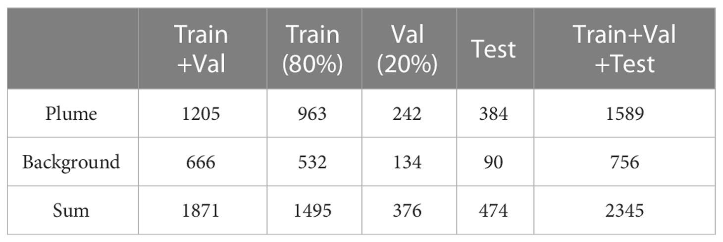
• We proposed a novel deep-sea hydrothermal plume dataset, which consists of 1589 images of the hydrothermal plume and 756 images of the seafloor background.

• We proposed a lightweight model based on the YOLOv5n algorithm to perform real-time plume detection. The original structure of YOLOv5n was improved in two aspects, including (1) replacing the SiLU activation functions with ReLU functions at shallow layers and Hard-SiLU functions at deep layers to increase the inference efficiency on the embedded system and (2) insetting an attention module termed Coordinate Attention (CA) into the backbone network to improve the overall accuracy.

• We adopted a transfer learning approach to utilize the knowledge learned from a fire and smoke dataset to better train the deep-sea hydrothermal plume detection model and enhance the model’s robustness and generalization.

• We deployed the proposed plume detection model on an embedded AI device NVIDIA Jetson TX2 NX using the TensorRT inference framework and achieved the real-time on-board high-accuracy plume detection.

2 Materials and methods

2.1 Object detection deep learning models

Deep learning in the machine vision field includes image classification, object detection, and instance segmentation. Object detection refers to the technique for recognizing and locating some specific objects in an image. As one of the primary tasks in machine vision, it has been extensively studied in the past few decades. In recent years, convolutional neural networks (CNNs) have gradually been the mainstream of object detection with the tremendous successes of deep learning in image classification (Liu et al., 2020). Generally, CNN-based object detection algorithms could be further classified into two-stage detectors and one-stage detectors (Wu et al., 2020). The former methods firstly generate the region proposals from input images and then do object classification and refinement for each region proposal. The latter innovatively reframe the object detection as a simple regression problem and perform the localization and classification in one network. Thus, one-stage methods normally have a better real-time performance.

Typical two-stage object detection methods are the R-CNN series, which include R-CNN (Girshick et al., 2014), Fast R-CNN (Girshick, 2015), and Faster R-CNN (Ren et al., 2015), etc. Representative one-stage object detection models are SSD (Liu et al., 2016) and YOLO series (including YOLO (Redmon et al., 2016), YOLOv2 (Redmon and Farhadi, 2017), YOLOv3 (Redmon and Farhadi, 2018), YOLOv4 (Bochkovskiy et al., 2020), and YOLOv5¹). YOLOv5 is the latest version of the YOLO series and its structure remains close to YOLOv4. The major difference between YOLOv4 and YOLOv5 is that they are developed in different deep learning frameworks. They are comparable in terms of accuracy, but YOLOv5 outperforms YOLOv4 in the aspect of speed and ease of model deployment. Unlike previous versions of YOLO developed in the Darknet², YOLOv5 is built in the PyTorch³ framework. Darknet is an open-source neural network framework written in C and CUDA. PyTorch, written in python, is much more easily configurable than Darknet, making YOLOv5 much more production ready.

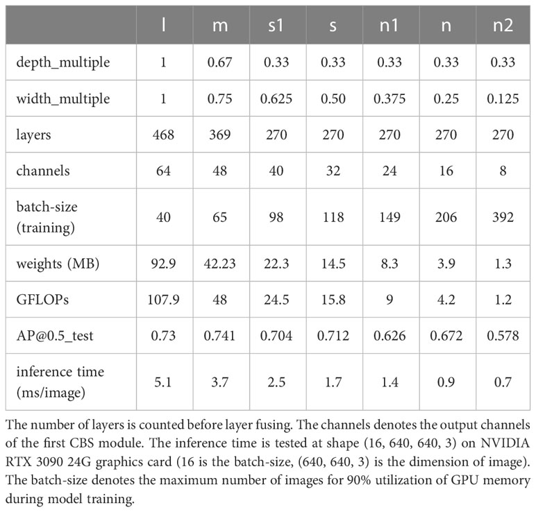
Like EfficientNet (Tan and Le, 2019), YOLOv5 adopts a simple yet effective compound scaling method that uniformly scales the network width and depth through a set of fixed scaling coefficients, called depth_multiple and width_multiple respectively. Based on differences in network depth and width, there are five models in the official release of YOLOv5-v6.1, named YOLOv5l, YOLOv5m, YOLOv5s, YOLOv5n, and YOLOv5x. Among them, YOLOv5l is the baseline model with both depth_multiple and width_multiple equal to 1, and the other four models are acquired at different scaling scales. Figure 1 shows the overall structure diagram of the YOLOv5-v6.1 series models. The CBS module is the basic module in YOLOv5-v6.1. It is composed of a 2D convolution (conv2d) layer, a batch normalization (BN) layer, and a sigmoid-weighted linear unit (SiLU) activation layer. YOLOv5 adopts CSPDarknet53 as the backbone and uses the same head as YOLOv3. Different from YOLOv4, YOLOv5 introduces the CSP network into PAN and then uses it as the neck. There are two kinds of CSP modules: the CSP in the backbone (noted as CSP1) and the CSP in the neck (noted as CSP2). The former consists of three CBS modules and several Bottleneck modules, while the latter only replaces a Bottleneck module with two CBS modules based on the former. It should be pointed out that the number of the Bottleneck modules is determined by the depth_multiple. In addition, YOLOv5 implements a new cascaded SPP module (called SPPF) that produces mathematically identical results to SPP with faster speeds. Finally, YOLOv5 has some small but useful tricks, such as the auto-learning bounding box anchors generating mechanism for custom datasets and the maximum batch-size auto-computing mechanism.

FIGURE 1

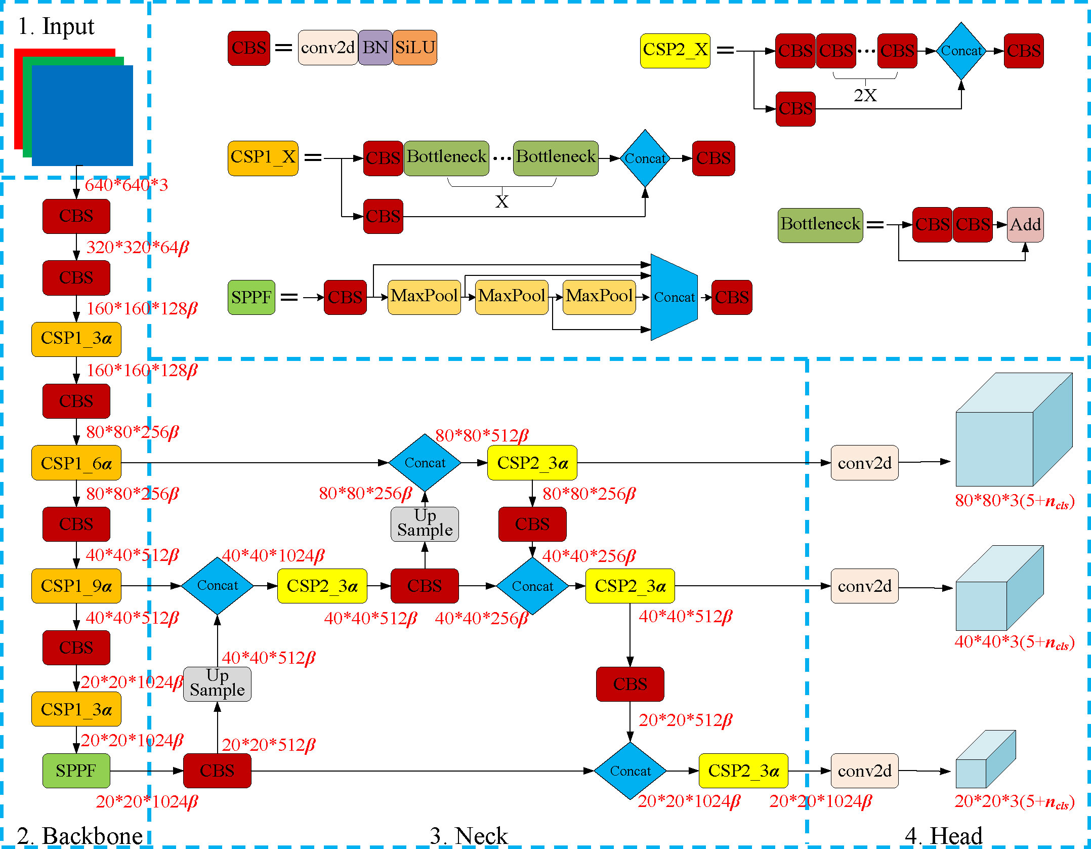
Figure 1 YOLOv5-v6.1 network structure diagram. α is the depth_multiple, β is the width_multiple, and n_clsis the number of object classes. 640*640*3, 320*320*64β etc. indicate the height*width*channels of the feature maps.

2.2 Deep-sea hydrothermal plume dataset

Deep Learning models are data-hungry for creating the best model or system with high performance. Finding or creating a quality dataset is a fundamental requirement for developing any real-world AI application. To our knowledge, there are currently no publicly available deep-sea hydrothermal plume datasets. As mentioned before, we have collected a lot of videos and images of the hydrothermal plume during the sampling process using ROV or HOV in the past few years. According to these private data and other small parts of images acquired from the internet, we built the first deep-sea hydrothermal plume dataset, consisting of 1589 images of the hydrothermal plume and 756 images of the deep-sea background. The plume dataset serves as a valuable resource for deep learning-based object detection model. Specifically, the background images are instrumental in training models to differentiate between areas with and without objects, which can reduce false positives and improve the accuracy of plume detection. Figure 2 shows some example images of the plume dataset.

FIGURE 2

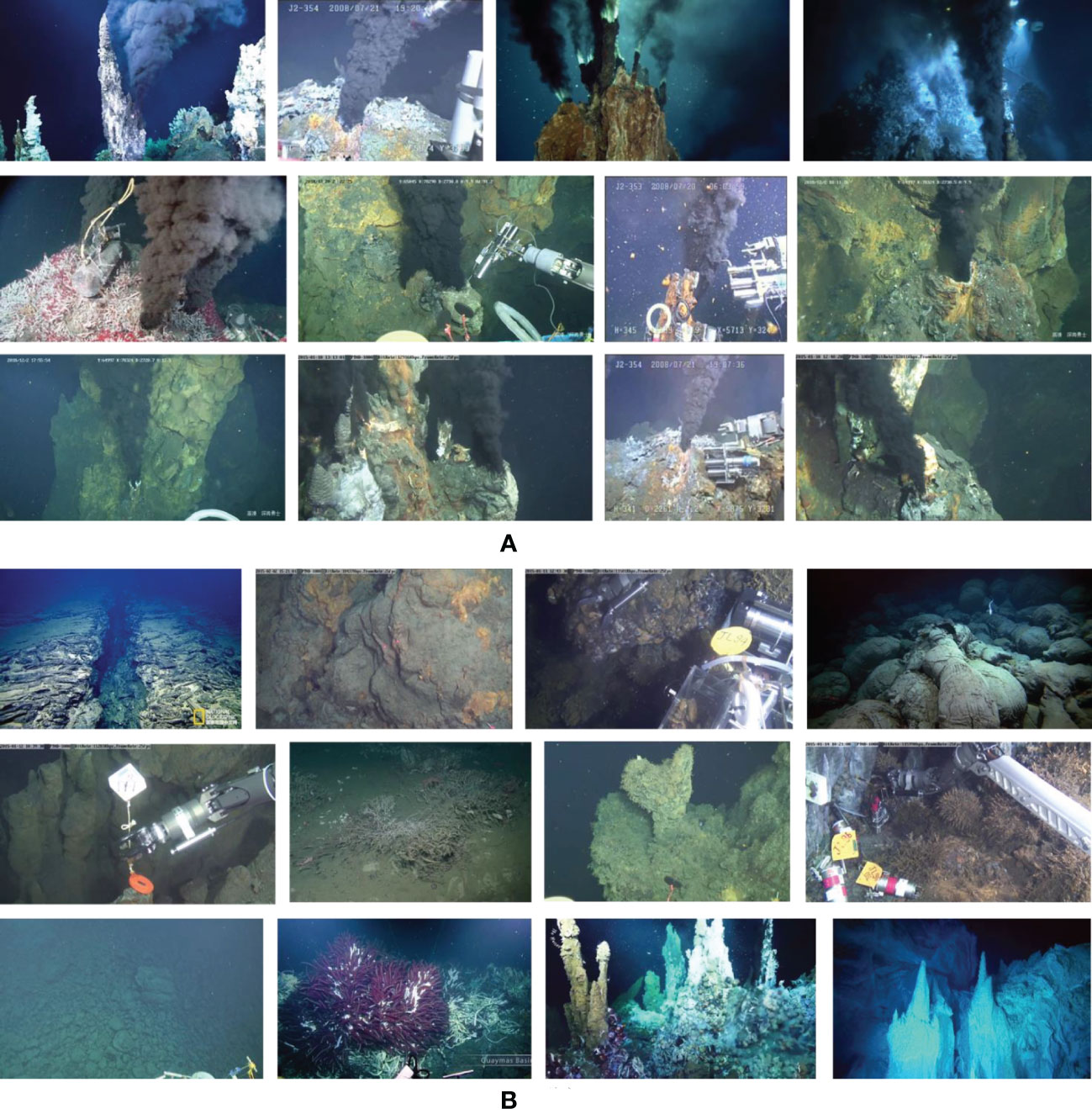
Figure 2 Example images from the deep-sea hydrothermal plume dataset: (A) images of hydrothermal plume; (B) images of deep-sea background.

2.2.1 Image extraction and labelling

The initial plume dataset contains about 60 videos filmed by ROV or HOV in different hydrothermal fields. In total there are approximately 10 h of video. We extracted 68 clips with hydrothermal plume target. Object detection models require still images with precisely labelled bounding boxes for training. However, the original video clips do not match the requirements. To meet the demands, we further extracted frames from these video clips at intervals of 2 seconds and then manually labelled the images using the LabelImg⁴ application. We saved these label files in the YOLO format, needed for YOLO models’ training. In addition, we wrote a python script to convert the YOLO format labels to the COCO format automatically. The COCO format labels are used to train and evaluate Faster-RCNN and SSD models developed in MMDetection open source object detection toolbox (Chen et al., 2019).

2.2.1 Dataset partitioning

All images and their corresponding labels were divided into 3 subsets, namely Train, Val, and Test. The former two subsets (also can be seen together as TrainVal set) are used for model training, while the latter one subset is used for final model performance evaluation. To better assess the trained model’s real performance, the images in the Test set and the images in the TrainVal set are from different videos. The numbers of images in different subsets of the plume dataset are shown in Table 1. We randomly picked 80% samples of the annotated images in the TrainVal set for model learning, with the remaining 20% used to form a validation set for best learning result assessment. Overfitting, which refers to a phenomenon that the model tries to fit the training data entirely and ends up performing poor in the case of unseen data scenarios, is a common problem in deep learning. We minimized overfitting by using the early-stopping technique. In our case, this was achieved by assessing the AP@0.5 on the Val set at intervals of one epoch and stopping the training when there were at least 50 epochs without improvement.

TABLE 1

Table 1 Numbers of images of different subsets in the deep-sea hydrothermal plume dataset.

2.2.3 Data augmentations

Deep convolutional neural networks have significantly improved the state of the arts on object detection machine vision tasks. However, their impressive performances are heavily reliant on massive amounts of labelled data for supervised learning. To improve the performance, we use the data augmentation technique to increase both the size and the diversity of the labelled plume dataset by leveraging label preserving transformations.

Common augmentations can be divided into two categories: geometric transformations and photometric transformations. Geometric transformations alter the geometry of the image to make the CNN insensitive to changes in position and orientation. Example transformations include flipping, cropping, scaling, translating, and rotating; As for photometric transformations, it adjusts the color channels or adds some noise to make the CNN insensitive to changes in illumination and color (Taylor and Nitschke, 2018). YOLOv5 not only contains these generic augmentations, but also has some unique augmentations such as Mosaic, MixUp, and Copy-Paste. However, it does not mean that the more data augmentation methods are used, the better the performance of the detector will be. For a specific dataset, it is necessary to choose some appropriate data augmentations. Obviously, flapping up-down is not practical in plume detection. In the proposed plume detector, we used a combination of Mosaic and some suitable traditional augmentation methods. To make the plume detector insensitive to changes in illumination and color, the enhancement coefficient of hue (H), saturation (S), and lightness (V) were set to 0.1, 0.8, and 0.5, respectively. Other coefficients were kept the same as those in YOLOv5.

2.3 Deep-sea hydrothermal plume detector

2.3.1 Model architecture

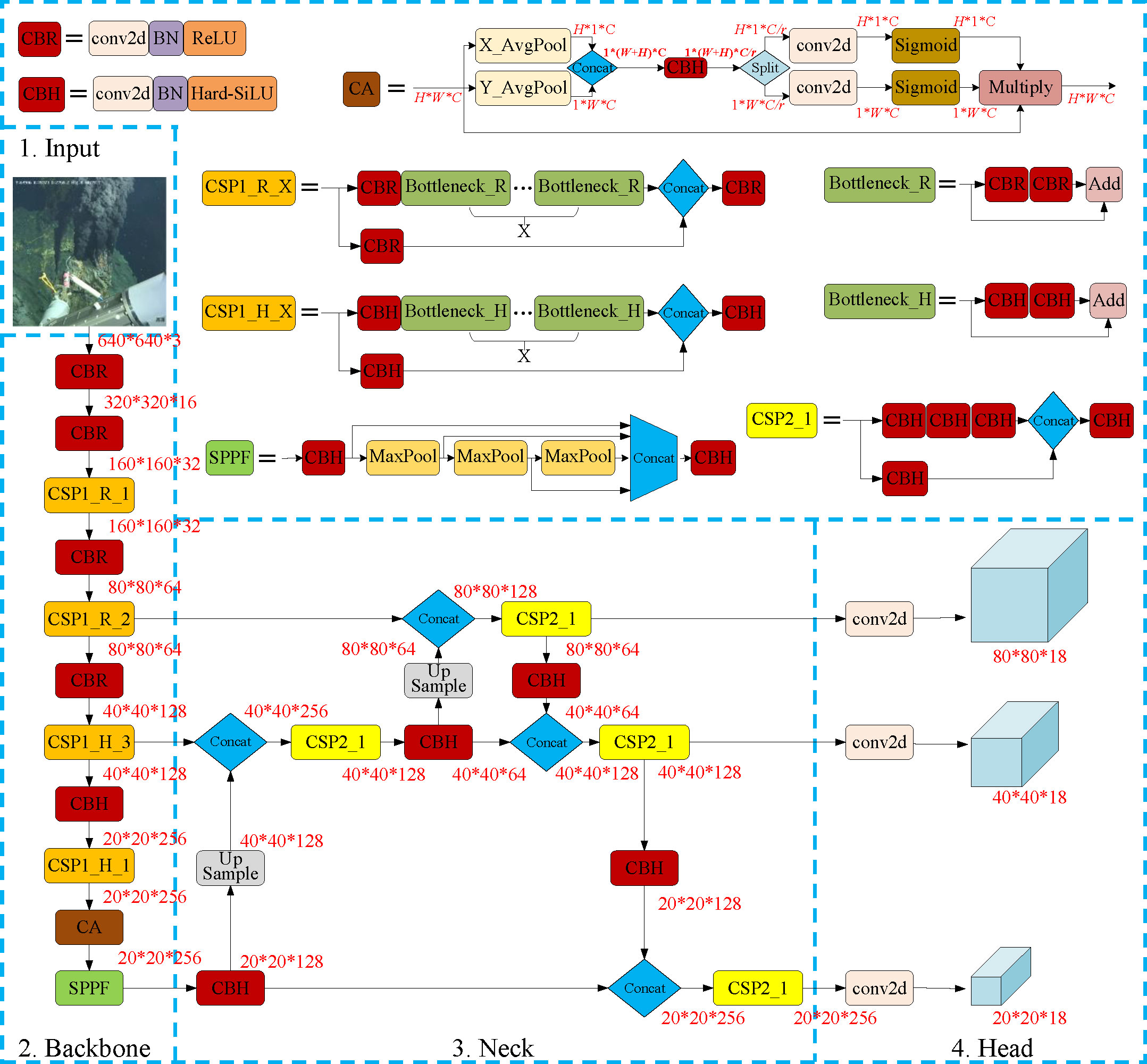
Prior studies have shown that network depth and width are both important for models’ expressive power. Normally, deeper CNN networks can capture richer and more complex features, and wider networks are capable of capturing more fine-grained features and are easier to train (Zagoruyko and Komodakis, 2016; Raghu et al., 2017). However, with the network getting deeper and wider, the number of weights increases and the inference speed goes slower. For a specific object detection task, choosing suitable depth and width is necessary for the trade-off between accuracy and efficiency. Through a comprehensive comparative experiment (related results are detailed in section 3.1), we finally chose to build the real-time deep-sea hydrothermal plume detector based on YOLOv5n. Furthermore, to accurately and efficiently detect hydrothermal plumes by using an embedded system, the original structure of YOLOv5n was improved in two aspects. First, SiLU activation functions in the model were replaced by ReLU at shallow layers and Hard-SiLU at deep layers to reduce the number of calculations (see section 2.3.1.1 for more details). Second, a CA attention module was integrated into the backbone network to improve the model’s sensitivity to channel and spatial features (see section 2.3.1.2 for more details). The architecture of the proposed hydrothermal plume detector is shown in Figure 3.

FIGURE 3

Figure 3 Network structure diagram of the proposed hydrothermal plume detector.

2.3.1.1 Activation functions

The choice of activation functions in deep neural networks has a significant effect on the training dynamics and task performance. Currently, the most successful and widely-used activation function is the Rectified Linear Unit (ReLU) (Nair and Hinton, 2010; Krizhevsky et al., 2017), defined as:

$\begin{array}{ll}\mathrm{Re}\text{LU}(x)=\{\begin{array}{cc}0,& x\le 0\\ x,& x>0\end{array}& (1)\end{array}$

Thanks to its simplicity and effectiveness, ReLU has become the default activation function used across the deep learning community. In YOLOv5, a nonlinearity called SiLU (Elfwing et al., 2018), also called Swish (Ramachandran et al., 2017), was employed as the activation function, which significantly improves the accuracy of neural networks. The activation of the SiLU is computed by the sigmoid function multiplied by its input. This nonlinearity is defined as:

$\begin{array}{ll}\text{SiLU}(x)=x·\sigma (x)=x·\frac{1}{1+e^{-x}}& (2)\end{array}$

where the $\sigma (x)=\frac{1}{1+e^{-x}}$ denotes the sigmoid function.

While this nonlinearity improves accuracy, it comes with a higher cost in embedded environments as the sigmoid function is much more expensive to compute than ReLU. Inspired by MobileNetV3 (Howard et al., 2019), we handled this problem by replacing the sigmoid function with its piece-wise linear hard analog $\frac{\text{ReLU6(}x+3)}{6}$, where

$\begin{array}{ll}\text{ReLU6(}x)=\{\begin{array}{cc}0,& x\le 0\\ x,& 0<x\le 6\\ 6,& x>6\end{array}& (3)\end{array}$

ReLU6 is a modification of the ReLU with a maximum size of 6. Similarly, the hard version of SiLU becomes:

$\begin{array}{ll}\text{ Hard-SiLU (}x)=x·\frac{\text{ReLU}6(x+3)}{6}=\{\begin{array}{cc}0,& x\le -3\\ \frac{x^2+3x}{6},& -3<x\le 3\\ x,& x>3\end{array}& (4)\end{array}$

The values of constants in Hard-SiLU was determined by being a good match to the original smooth version. Replacing SiLU with Hard-SiLU has no discernible difference in accuracy, but the piece-wise implementation of Hard-SiLU can reduce the number of memory accesses, improving the training and inference efficiency substantially. In addition, since most of the benefits of SiLU are obtained by using them only in the deeper layers, Hard-SiLU was only used in the deep layers in our modified model architecture. We replaced SiLU activations in the shallow layers with more simple ReLU activations to further reduce the calculation.

2.3.1.2 Attention modules

Attention modules, inspired by the attention mechanisms in the human brain, have been widely used for boosting the performance of modern deep neural networks, thanks to their ability to provide additional information on “where” and “what” to focus on. However, their application for lightweight networks deployed in the embedded systems with limited computing power significantly lags behind that for large networks running in the workstation with powerful and expensive GPU graphics cards. This is mainly because the computational overhead brought by most attention modules is not affordable for embedded devices. Considering the restricted computation competence of embedded systems, to date, the most popular attention mechanisms for lightweight neural networks are still the Squeeze-and-Excitation (SE) (Hu et al., 2018), Convolutional Block Attention Module (CBAM) (Woo et al., 2018), and Coordinate Attention (CA) (Hou et al., 2021). Among them, the SE attention only considers encoding inter-channel information but neglects the position information. The CBAM network exploits positional information by reducing the channel dimension of the input tensor and then computing spatial attention using convolutions. However, convolutions can only capture local relations but fail in modeling long-range dependencies. The CA module embeds positional information into channel attention to attend over large regions. It can capture not only cross-channel but also position-sensitive information and generates coordinate-aware attention maps while avoiding increasing significant computation overhead. A previous study demonstrates that the CA module outperforms the SE and CBAM in object detection tasks (Hou et al., 2021). Thus, we inserted a CA module in the plume detector’s backbone network to lift its performance.

The block diagram of the CA module is shown at the top of Figure 3. Unlike channel attention that converts a feature tensor to a single feature vector via 2D global pooling, the CA module employs two 1D global pooling operations to respectively aggregate the input features map X (dimension is H*W*C) along the vertical and horizontal directions into two separate direction-aware feature maps X1 (dimension is H*1*C) and X2 (dimension is 1*W*C). These two feature maps embedded with direction-specific information are then concatenated to form feature map X3 (dimension of 1*(H+W)*C) which is subsequently passed through a CBH module. The CBH module reduces the channels from C to C/r based on a specified reduction ratio r (in our implementation, r was set to 32). After that, the feature map acquired is split into two tensors which are then individually passed through two 2D convolution kernels to increase the channels back to C from C/r. Finally, two sigmoid activations are separately applied on the resultant two tensors to form the two attention maps, each of which captures long-range dependencies of the input feature map along one spatial direction. Therefore, the positional information can be preserved in the generated attention maps. The two attention maps are then sequentially element-wise multiplied with the original input feature map to emphasize the representations of interest. The dimension of the feature map does not change after it was processed by the CA module. Thus, it is convenient to plug the CA module into any classic deep neural network.

2.3.2 Model training and deployment

After preparing the plume dataset and defining the model’s structure, we trained the plume detector in the Pytorch deep learning framework. A weights file was obtained after the training. For model deployment on Jetson TX2 NX, we firstly rebuilt the plume detector by the NVIDIA TensorRT C++ API and then generated the plume detection TensorRT engine file with the weights file obtained in the model training process. The detailed flow chart of the proposed plume detection method including model training and deployment process has been shown in Figure 4.

FIGURE 4

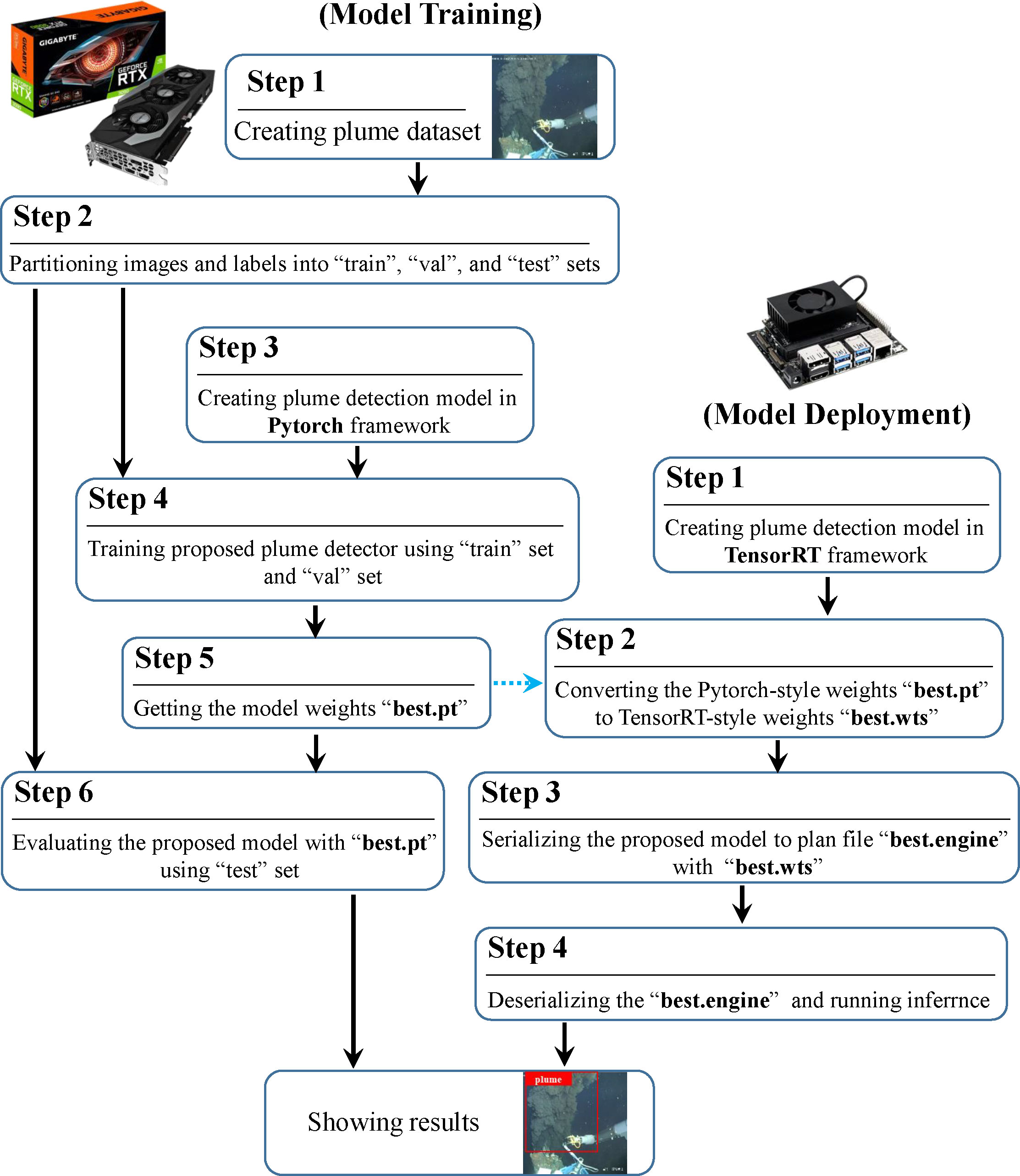
Figure 4 Flow chart of the proposed method, including model training (left) and model deployment (right) two parts.

2.3.2.1 Model training platform

A workstation running the Ubuntu 20.04 operating system was used as the model training platform. The Pytorch framework and the proposed plume detection algorithm were built in the Anaconda3 environment. The program was written in Python 3.7, and the CUDA version was 11.1. For hardware, the processor was an AMD 64-Core Ryzen Threadripper Pro 3995WX with 3.5 GHz main frequency, the memory was 126G, and the graphics card was a GeForce RTX 3090 24G.

2.3.2.2 Training with transfer learning

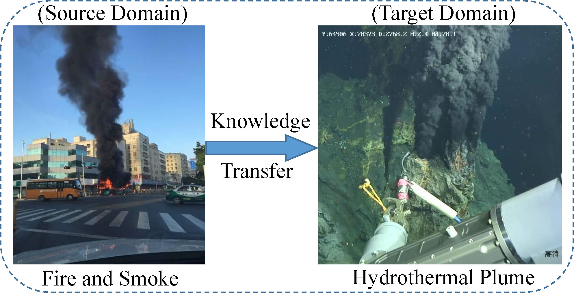
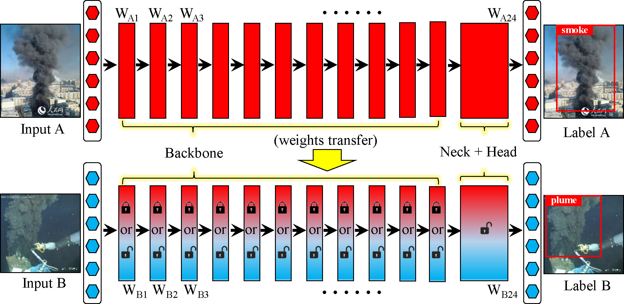
Transfer learning, inspired by human beings’ capabilities to transfer knowledge across domains, is an effective model training method that can leverage knowledge from a different but related source domain to improve the performance of target learners in a specific target domain where labelled data is scarce (Zhuang et al., 2020). As we described before, there are no open-source deep-sea hydrothermal plume datasets. The plume dataset created by ourselves only contains 2345 images in total. For training of deep learning models, it is not large enough. Although the data augmentation technique can rich the plume dataset to a certain extent, its improvement is still limited. Thus, we further utilized the transfer learning method to boost the plume detector’s performance. As can be seen in Figure 5, the deep-sea hydrothermal plume is very similar in shape, texture, and color to the smoke on land. After searching, a fire and smoke dataset⁵, consisting of 23.7k images, was found in the Kaggle community. We treated the fire and smoke dataset as the source domain in our transfer learning experiment.

FIGURE 5

Figure 5 Schematic diagram of the knowledge transfer.

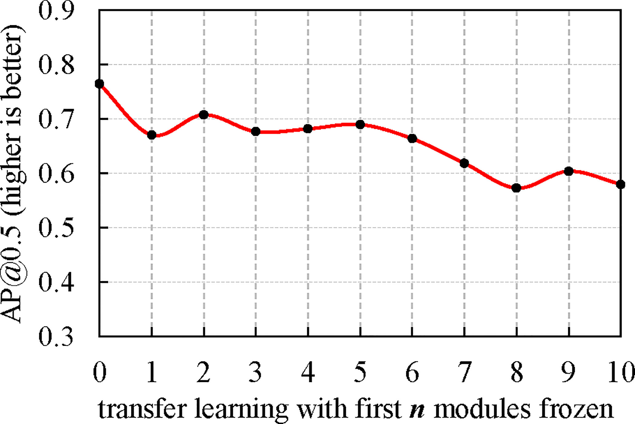
The transfer learning method commonly used in the field of deep learning is to copy the weights of the base network trained on the source dataset to the target network, and then train the target network on the target dataset. For the transferred weights, there are two methods to deal with: fine-tuning or freezing. The former method backpropagates the errors from the new task into the copied features to fine-tune them to the new task. The latter method leaves the transferred feature layers frozen in place, meaning that the copied features do not update during training on the new task. How to handle the copied features of the target network is determined by the size of the target dataset and the number of parameters of the network. On the one hand, when the number of parameters is large and the target dataset is small, an overfitting phenomenon may occur if only fine-tune the transferred features, so some of the weights (first n layers) can be left frozen. On the other hand, when the target dataset is large or the number of parameters is small, there are enough data for parameter update to make that overfitting do not happen, so all the copied features can be fine-tuned to the new task to boost performance. Of course, if the target dataset is very large, there would be no need to utilize the transfer learning method since the labelled images in the dataset are rich enough for model training from scratch (Yosinski et al., 2014). In our case, we conducted some comparative experiments to do a better choice. An overview of the experimental treatments and controls of the transfer learning method is shown in Figure 6. Through experiments, we found that the best detection performance was obtained by only fine-tuning the target network with no need for freezing the first n layers. Although the plume dataset is not very large, our proposed plume detector is a lightweight network with few parameters, so this result is reasonable. The detailed experimental results can be seen in section 3.4.

FIGURE 6

Figure 6 Overview of experimental treatments and controls of the transfer learning.

2.3.2.3 Model deployment platform

NVIDIA Jetson TX2 NX⁶ is a powerful but compact embedded product. It provides up to 1.33 TFLOPs AI performance, which is 2.5 times the performance of Jetson Nano. Jetson TX2 NX shares form-factor and pin compatibility with Jetson Nano. It consists of an NVIDIA Pascal architecture GPU with 256 CUDA cores, a CPU complex with Denver 2 (Dual-Core) processor and ARM Cortex-A57 MPcore (Quad-Core) processor, and a 4GB-128bit-LPDDR4 memory. Thanks to its high performance, low power consumption, and small form-factor, Jetson TX2 NX is a preferred hardware platform to deploy a hydrothermal plume detection model for AUV with limited space and constrained battery. The trained plume detection model has been transplanted into the Jetson TX2 NX using the TensorRT⁷ inference engine, a C++ library for high-performance inference on NVIDIA GPUs.

3 Results

3.1 Performances of different scale models of YOLOv5

To find a suitable baseline model for real-time plume detection, besides the officially released four models (YOLOv5 l, m, s, n), we still trained and tested three custom models (named YOLOv5 s1, n1, n2) on the plume dataset. The tested seven models have a similar structure with only differences in depth (layers) and width (channels). In this experiment, the number of training epochs was set to 600, and the optimal batch-size, which refers to the number of training examples utilized in one iteration, was auto-computed for the 90% utilization of GPU memory. All the hyper-parameters used were the default values in the hyp.scratch-low.yaml⁸ file.

The parameters and plume detection performances of different scale models of YOLOv5 are detailed in Table 2. From Table 2, the following conclusions can be drawn:

• As the network gets deeper and wider, the required inference time increases dramatically.

• In general, large models have better accuracy performance in plume detection than small models, but the difference is not as big as that of inference time.

• Reducing the computation of model, the maximum batch-size that GPU can support increases.

• To balance accuracy and efficiency, YOLOv5n is a better choice for building the plume detector. Compared with YOLOv5m, it only has a slight loss of accuracy (0.069 AP decrease, i.e., from 0.741 to 0.672) but almost 4 times increase of inference speed (i.e., from 3.7 ms/image to 0.9 ms/image). Compared with YOLOv5n2, it has comparable speed but much higher accuracy performance.

TABLE 2

Table 2 Plume detection performance comparisons between different scale models of YOLOv5-v6.1.

3.2 The effectiveness of CA module

For the qualitative analysis of the CA module’s impact on the performance of the plume detector, we apply the Grad-CAM as our visualization tool to visualize the class activation maps of models with and without attention mechanism. Grad-CAM is a recently proposed visualization method that uses gradients to calculate the importance of the spatial locations in convolutional layers (Selvaraju et al., 2017). The visualization results of Grad-CAM can clearly illustrate the attended regions of models. Figure 7A is the original input image with ground truth marked, Figure 7B shows the Grad-CAM heat-map and predicted plume bounding box produced by the baseline model (YOLOv5n), and Figure 7C displays the visualization results of the model with the CA module integrated (YOLOv5n+CA). It is evident that the Grad-CAM mask of the CA-integrated model can more precisely cover the target plume region than that of the model without the CA module, which fully reveals the CA module’s effectiveness in promoting the plume detector to exploit information in target object regions. Consequently, the CA module improves the prediction of the plume bounding box. For the quantitative analysis, the CA-integrated model outperforms the baseline model by 3.1% AP (from 0.672 to 0.703) with only a bit of parameters increase (from 1.76M to 1.77M).

FIGURE 7

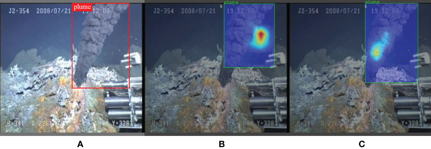
Figure 7 Grad-CAM visualization results. (A) The input image with ground truth marked. (B) The visualization result of baseline model (YOLOv5n). (C) The visualization result of CA-integrated model (YOLOv5n+CA).

3.3 The effectiveness of activations

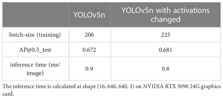
Table 3 shows the ablation study of YOLOv5n with and without activations changed. From Table 3, one can find that replacing SiLU with Hard-SiLU can guarantee a larger batch-size under the same GPU memory condition and less inference time, which confirms that the Hard-SiLU activation can offer a model with reduced memory utilization and computation. In addition, there is even a slight increase in the AP performance, which indicates that replacing SiLU with Hard-SiLU has no discernible difference in accuracy.

TABLE 3

Table 3 The ablation study of YOLOv5n with and without activations changed.

3.4 The effectiveness of transfer learning

In the transfer learning experiments, we first trained the improved YOLOv5n model (i.e., our proposed model) on the fire and smoke dataset for 600 epochs. After about 12 hours of training, a weights file of about 3.9 MB in size was obtained. Subsequently, we trained the improved YOLOv5n model on the custom-made deep-sea hydrothermal plume dataset with loading the fire and smoke pre-trained weights. We choose to freeze the first n (from 0 to 10) modules of the model and then see the performance differences in different situations. Figure 8 shows the results of this transfer learning experiment. From Figure 8, one can see that the best AP performance can be obtained by only fine-tuning the target network without freezing. With transfer learning, we achieved the best AP of 0.765.

FIGURE 8

Figure 8 Results of the transfer learning experiment.

3.5 Comparisons with state-of-the-arts (other alternatives)

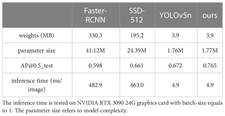
Table 4 shows the performance comparisons of our proposed plume detector with the other three state-of-the-art methods. One can see that our proposed plume detector outperforms Faster-RCNN and SSD-512 in both accuracy and inference speed. Compared to the baseline model YOLOv5n, our model can make a 9.3% AP improvement (i.e., from 0.672 to 0.765) and requires the same inference time, which fully reveals that our improved plume detector can not only maintain a good performance of efficiency but also achieves a tremendous increase in detection accuracy.

TABLE 4

Table 4 The comparison results with other state-of-the-art methods.

3.6 Test results on Jetson TX2 NX

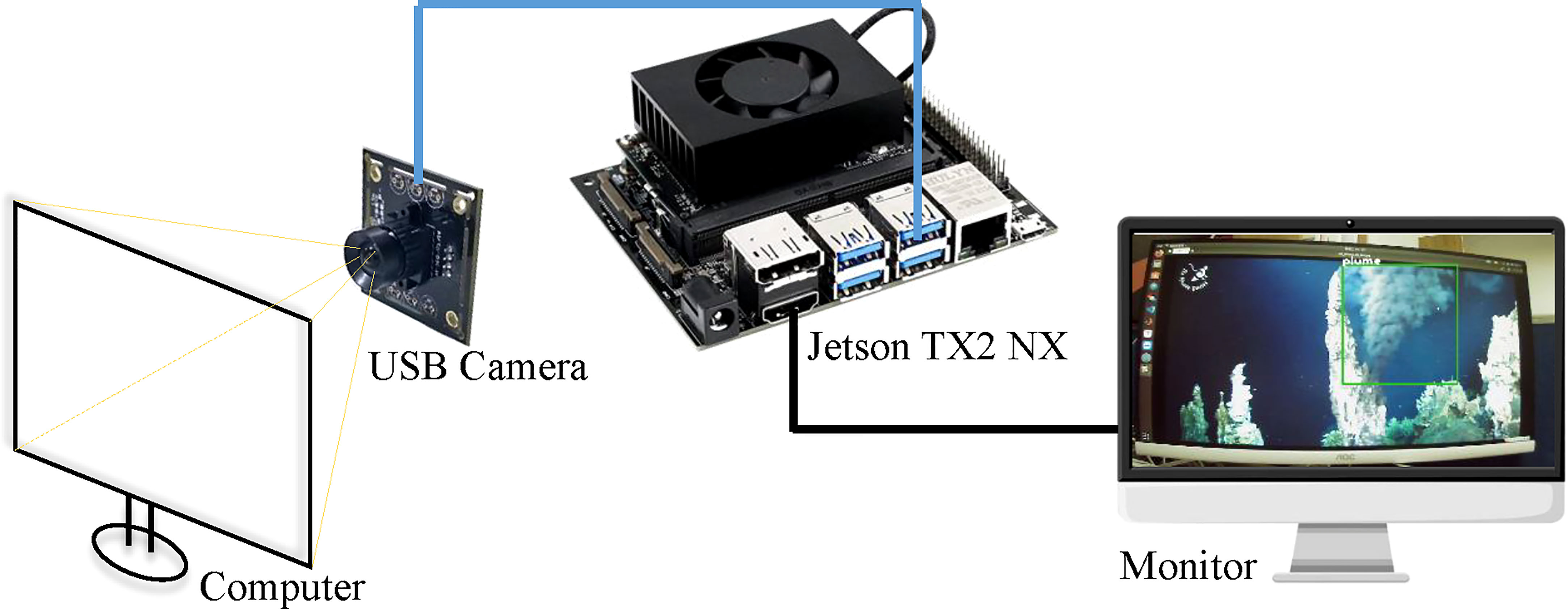
We tested the deployed plume detector as a stand-alone application in Jetson TX2 NX to evaluate its final application performance. As shown in Figure 9, a USB camera and a monitor are connected to the Jetson TX2 NX. The camera was exposed to another computer that was playing a video with the target of the deep-sea hydrothermal plume. The monitor was used to present the detection results. we recorded various parameters when the proposed plume detector was running in the Jetson TX2 NX. The resolution of the USB camera is 640x480. Although this camera only supports a 30 fps frame rate at this resolution, the video processing speed of the plume detector calculated was about 37 fps. It should be noted that we take not only the inference time but also the pre-processing and post-processing into account to calculate the fps. The pre-processing includes converting BGR to RGB and resizing the image to 640x640. The post-processing includes non-maximum suppression (NMS) processing of the predicted bounding box and putting the final bounding box on the image. The real-time on-board detection capability of the proposed plume detector is demonstrated. During the test, the power consumption and GPU temperature of the Jetson TX2 NX were also measured using jtop⁹, a system monitoring utility. The power consumption was 2.58 W on average and the temperature was 40.5°C when the plume detector was off. While our method was executed, the power consumption was 4.02 W and the temperature was 49.5°C. Thus, the power consumption of our proposed plume detector is only 1.44 W, which benefits a lot for application in battery-powered devices.

FIGURE 9

Figure 9 Testing the proposed plume detector on Jetson TX2 NX.

3.7 Plume detection test in water tank with AUV

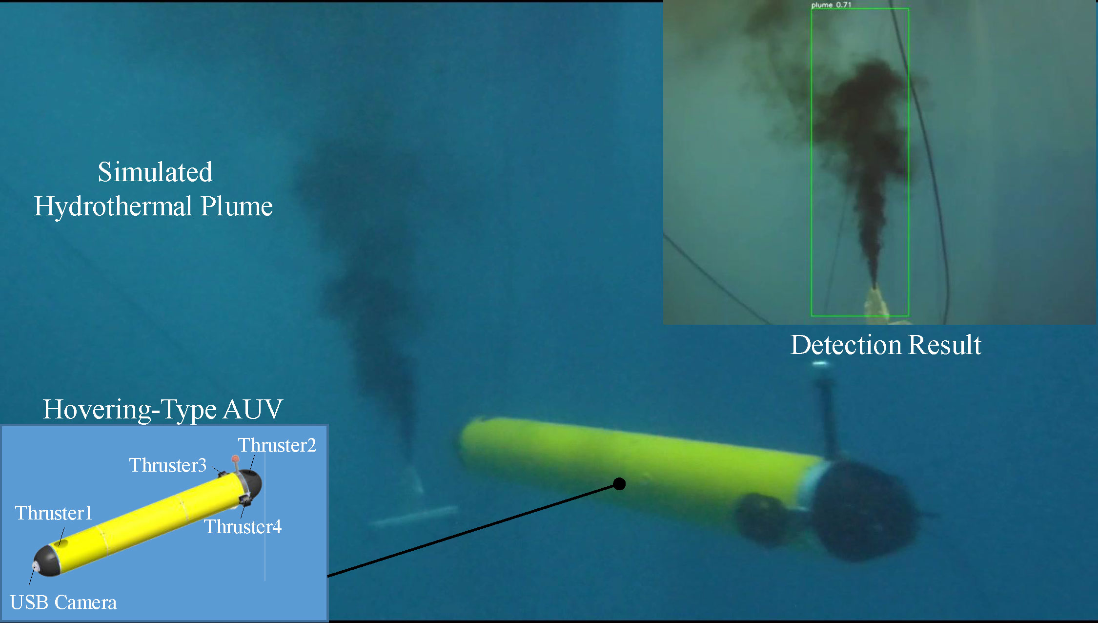
We then installed the Jetson TX2 NX into a hovering-type AUV as its vision processing unit. A water tank test was conducted in the laboratory. As shown in Figure 10, we simulated a dynamic hydrothermal plume in the water tank, and then used the hovering-type AUV to explore it. The experimental results show that our proposed hydrothermal plume detector can endow the AUV with the ability of real-time and intelligent detection of the hydrothermal plume. Based on the detection result, we also designed an image-based visual servo (IBVS) algorithm to help the AUV approach the target automatically and did some tests in the water tank. Since that is out of the scope of this paper, we will present the related results in another paper.

FIGURE 10

Figure 10 Water tank test of a hovering-type AUV configured with the proposed plume detector.

4 Conclusion and discussion

This paper proposed a real-time and embedded implementation of the deep-sea hydrothermal plume detection technique that can give AUV the competence of intelligent hydrothermal plume detection. The proposed solution achieved more promising results for accuracy and efficiency performance compared to other state-of-the-art methods. The preliminary water tank test verified the feasibility of the proposed method and laid the foundation for the accurate detection or sampling of deep-sea hydrothermal plumes by using AUV. However, only the static spatial features are considered in our proposed plume detector now, as only the still images are used for training. In the future, we will further improve our algorithm by taking the dynamic and temporal characteristics of the hydrothermal plume into account. One possible method is to combine CNNs and LSTM (long short-term memory) neural networks in a consecutive way so that the model can learn the dynamic and temporal features of the hydrothermal plume. However, the LSTM usually causes high computational costs. How to make this method be practically used on AUV needs to be further studied. Finally, we will extend our research to deploy the proposed plume detection system on an AUV for achieving automatic plume sampling by providing real-time visual status and feedback on the hydrothermal plumes in actual sea trials.

Data availability statement

The raw data supporting the conclusions of this article will be made available by the authors, without undue reservation.

Author contributions

SW and CY designed the study. XW created the plume dataset and performed the experiments and drafted the manuscript. YC and SW proofread the manuscript and gave valuable advice. All authors contributed to the article and approved the submitted version.

Funding

This work is supported by the National Science Foundation of Zhejiang Province, China (Grant No. LR21E090001) and the National Natural Science Foundation of China (Grant No. 51879232).

Acknowledgments

Most of the videos in our hydrothermal plume dataset are captured during the past research cruises we have attended, which include the cruise of KNOX18RR with the R/V Roger Revelle and the ROV Jason, the cruise of DY35 with R/V Xiang Yang Hong 09 and HOV Jiaolong, and the cruise of TS 10 with R/V Tan Suo Yi Hao and HOV Shen Hai Yong Shi, etc. We are grateful to all the crews for their support during these cruises.

Conflict of interest

The authors declare that the research was conducted in the absence of any commercial or financial relationships that could be construed as a potential conflict of interest.

Publisher’s note

All claims expressed in this article are solely those of the authors and do not necessarily represent those of their affiliated organizations, or those of the publisher, the editors and the reviewers. Any product that may be evaluated in this article, or claim that may be made by its manufacturer, is not guaranteed or endorsed by the publisher.

Supplementary material

The Supplementary Material for this article can be found online at: https://www.frontiersin.org/articles/10.3389/fmars.2023.1124185/full#supplementary-material

Footnotes

1. ^ https://github.com/ultralytics/yolov5
2. ^ https://pjreddie.com/darknet/
3. ^ https://pytorch.org/
4. ^ https://github.com/heartexlabs/labelImg
5. ^ https://www.kaggle.com/datasets/hhhhhhdoge/fire-smoke-dataset
6. ^ https://developer.nvidia.com/embedded/jetson-tx2-nx
7. ^ https://github.com/NVIDIA/TensorRT
8. ^ https://github.com/ultralytics/yolov5/blob/master/data/hyps/hyp.scratch-low.yaml
9. ^ https://github.com/rbonghi/jetson_stats

References

Bochkovskiy A., Wang C. Y., Liao H. Y. M. (2020). “Yolov4: Optimal speed and accuracy of object detection,” in arXiv. doi: 10.48550/arXiv.2004.10934

CrossRef Full Text | Google Scholar

Chen K., Wang J., Pang J., Cao Y., Xiong Y., Li X., et al. (2019). “MMDetection: Open mmlab detection toolbox and benchmark,” in arXiv. doi: 10.48550/arXiv.1906.07155

CrossRef Full Text | Google Scholar

Chen Y., Wu S., Xie Y., Yang C., Zhang J. (2007). A novel mechanical gas-tight sampler for hydrothermal fluids. IEEE J. Oceanic Eng. 32 (3), 603–608. doi: 10.1109/joe.2007.891887

CrossRef Full Text | Google Scholar

Corliss J. B., Dymond J., Gordon L. I., Edmond J. M., von Herzen R. P., Ballard R.D., et al. (1979). Submarine thermal springs on the Galapagos rift. Sci. 203 (4385), 1073–1083. doi: 10.1126/science.205.4409.856.d

CrossRef Full Text | Google Scholar

Ditria E. M., Lopez-Marcano S., Sievers M., Jinks E. L., Brown C. J., Connolly R. M. (2020). Automating the analysis of fish abundance using object detection: Optimizing animal ecology with deep learning. Front. Mar. Sci. 429. doi: 10.3389/fmars.2020.00429

CrossRef Full Text | Google Scholar

Elfwing S., Uchibe E., Doya K. (2018). Sigmoid-weighted linear units for neural network function approximation in reinforcement learning. Neural Networks 107, 3–11. doi: 10.1016/j.neunet.2017.12.012

PubMed Abstract | CrossRef Full Text | Google Scholar

German C. R., Yoerger D. R., Jakuba M., Shank T. M., Langmuir C. H., Nakamura K. I. (2008). Hydrothermal exploration with the autonomous benthic explorer. Deep Sea Res. Part I 55 (2), 203–219. doi: 10.1016/j.dsr.2007.11.004

CrossRef Full Text | Google Scholar

Girshick R. (2015). “Fast r-cnn,” in Proceedings of the IEEE international conference on computer vision (Santiago: IEEE), 1440–1448. doi: 10.1109/iccv.2015.169

CrossRef Full Text | Google Scholar

Girshick R., Donahue J., Darrell T., Malik J. (2014). “Rich feature hierarchies for accurate object detection and semantic segmentation,” in Proceedings of the IEEE conference on computer vision and pattern recognition (Columbus: IEEE), 580–587. doi: 10.1109/cvpr.2014.81

CrossRef Full Text | Google Scholar

Hou Q., Zhou D., Feng J. (2021). “Coordinate attention for efficient mobile network design,” in Proceedings of the IEEE/CVF conference on computer vision and pattern recognition (Virtual: IEEE), 13713–13722. doi: 10.1109/cvpr46437.2021.01350

CrossRef Full Text | Google Scholar

Howard A., Sandler M., Chu G., Chen L. C., Chen B., Tan M., et al. (2019). “Searching for mobilenetv3,” in Proceedings of the IEEE/CVF international conference on computer vision (Seoul: IEEE), 1314–1324. doi: 10.1109/iccv.2019.00140

CrossRef Full Text | Google Scholar

Hu J., Shen L., Sun G. (2018). “Squeeze-and-excitation networks,” in. Proc. IEEE Conf. Comput. Vision Pattern recognition (Salt Lake City: IEEE), 7132–7141. doi: 10.1109/cvpr.2018.00745

CrossRef Full Text | Google Scholar

Kandimalla V., Richard M., Smith F., Quirion J., Torgo L., Whidden C. (2022). Automated detection, classification and counting of fish in fish passages with deep learning. Front. Mar. Sci. 2049. doi: 10.3389/fmars.2021.823173

CrossRef Full Text | Google Scholar

Krizhevsky A., Sutskever I., Hinton G. E. (2012). Imagenet classification with deep convolutional neural networks. Communications of the ACM, 60 (6), 84–90. doi: 10.1145/3065386

CrossRef Full Text | Google Scholar

Kumagai H., Tsukioka S., Yamamoto H., Tsuji T., Shitashima K., Asada M., et al. (2010). Hydrothermal plumes imaged by high-resolution side-scan sonar on a cruising AUV, urashima. Geochem., Geophys. Geosyst. 11 (12). doi: 10.1029/2010gc003337

CrossRef Full Text | Google Scholar

Li Y., Guo J., Guo X., Zhao J., Yang Y., Hu Z., et al. (2021). Toward in situ zooplankton detection with a densely connected YOLOV3 model. Appl. Ocean Res. 114, 102783. doi: 10.1016/j.apor.2021.102783

CrossRef Full Text | Google Scholar

Liao W., Zhang S., Wu Y., An D., Wei Y. (2022). Research on intelligent damage detection of far-sea cage based on machine vision and deep learning. Aquac. Eng. 96, 102219. doi: 10.1016/j.aquaeng.2021.102219

CrossRef Full Text | Google Scholar

Liu W., Anguelov D., Erhan D., Szegedy C., Reed S., Fu C. Y., et al. (2016). “Ssd: Single shot multibox detector,” in European Conference on computer vision (Amsterdam: Springer), 21–37. doi: 10.1007/978-3-319-46448-0_2

CrossRef Full Text | Google Scholar

Liu L., Ouyang W., Wang X., Fieguth P., Chen J., Liu X., et al. (2020). Deep learning for generic object detection: A survey. Int. J. Comput. Vision 128 (2), 261–318. doi: 10.1007/s11263-019-01247-4

CrossRef Full Text | Google Scholar

Luther G. W., Rozan T. F., Taillefert M., Nuzzio D. B., Di Meo C., Shank T. M., et al. (2001). Chemical speciation drives hydrothermal vent ecology. Nat. 410 (6830), 813–816. doi: 10.1038/35071069

CrossRef Full Text | Google Scholar

Minami H., Ohara Y. (2020). Tectonic, volcanic and hydrothermal features of a nascent rift graben in the southern Okinawa trough. Mar. Geo. 430, 106348. doi: 10.1038/s41467-020-15062-w

CrossRef Full Text | Google Scholar

Nair V., Hinton G. E. (2010). “Rectified linear units improve restricted boltzmann machines,” in Icml (Haifa: Omnipress), 807–814.

Google Scholar

Okamoto A., Seta T., Sasano M., Inoue S., Ura T. (2019). Visual and autonomous survey of hydrothermal vents using a hovering-type AUV: Launching hobalin into the Western offshore of kumejima island. Geochem. Geophys. 20 (12), 6234–6243. doi: 10.1029/2019gc008406

CrossRef Full Text | Google Scholar

Petersen J. M., Zielinski F. U., Pape T., Seifert R., Moraru C., Amann R., et al. (2011). Hydrogen is an energy source for hydrothermal vent symbioses. Nat. 476 (7359), 176–180. doi: 10.1038/nature10325

CrossRef Full Text | Google Scholar

Raghu M., Poole B., Kleinberg J., Ganguli S., Sohl-Dickstein J. (2017). “On the expressive power of deep neural networks,” in International conference on machine learning, 2847–2854.

Google Scholar

Ramachandran P., Zoph B., Le Q. V. (2017). “Searching for activation functions,” in arXiv. doi: 10.48550/arXiv.1710.05941

CrossRef Full Text | Google Scholar

Redmon J., Divvala S., Girshick R., Farhadi A. (2016). “You only look once: Unified, real-time object detection,” in Proceedings of the IEEE conference on computer vision and pattern recognition (Las Vegas: IEEE), 779–788. doi: 10.1109/cvpr.2016.91

CrossRef Full Text | Google Scholar

Redmon J., Farhadi A. (2017). “YOLO9000: better, faster, stronger,” in Proceedings of the IEEE conference on computer vision and pattern recognition (Honolulu: IEEE), 7263–7271. doi: 10.1109/cvpr.2017.690

CrossRef Full Text | Google Scholar

Redmon J., Farhadi A. (2018). “Yolov3: An incremental improvement,” in arXiv. doi: 10.48550/arXiv.1804.02767

CrossRef Full Text | Google Scholar

Ren S., He K., Girshick R., Sun J. (2015). Faster r-cnn: Towards real-time object detection with region proposal networks. Adv. Neural Inf. Process. Syst. 28. doi: 10.1109/tpami.2016.2577031

CrossRef Full Text | Google Scholar

Seewald J. S., Doherty K. W., Hammar T. R., Liberatore S. P. (2002). A new gas-tight isobaric sampler for hydrothermal fluids. Deep Sea Res. Part I 49 (1), 189–196. doi: 10.1016/s0967-0637(01)00046-2

CrossRef Full Text | Google Scholar

Selvaraju R. R., Cogswell M., Das A., Vedantam R., Parikh D., Batra D. (2017). “Grad-cam: Visual explanations from deep networks via gradient-based localization,” in Proceedings of the IEEE international conference on computer vision (Venice: IEEE), 618–626. doi: 10.1109/iccv.2017.74

CrossRef Full Text | Google Scholar

Tan M., Le Q. (2019). “Efficientnet: Rethinking model scaling for convolutional neural networks,” in International conference on machine learning (Long Beach: PMLR), 6105–6114.

Google Scholar

Tao C., Seyfried W. E. Jr., Lowell R. P., Liu Y., Liang J., Guo Z., et al. (2020). Deep high-temperature hydrothermal circulation in a detachment faulting system on the ultra-slow spreading ridge. Nat. com. 11 (1), 1300. doi: 10.1038/s41467-020-15062-w

CrossRef Full Text | Google Scholar

Taylor L., Nitschke G. (2018). “Improving deep learning with generic data augmentation,” in 2018 IEEE symposium series on computational intelligence (SSCI) (Bangalore: IEEE), 1542–1547. doi: 10.1109/ssci.2018.8628742

CrossRef Full Text | Google Scholar

Wang X., Wu S. J., Fang Z. F., Yang C. J., Wang S. (2020). A pressure-tight sampler with flexible titanium bag for deep-Sea hydrothermal fluid samples. J. Atmos. Oceanic Technol. 37 (11), 2065–2073. doi: 10.1175/jtech-d-20-0017.1

CrossRef Full Text | Google Scholar

Woo S., Park J., Lee J. Y., Kweon I. S. (2018). “Cbam: Convolutional block attention module,” in Proceedings of the European conference on computer vision (ECCV) (Munich: Springer), 3–19. doi: 10.1007/978-3-030-01234-2_1

CrossRef Full Text | Google Scholar

Wu X., Sahoo D., Hoi S. C. (2020). Recent advances in deep learning for object detection. Neurocomputing 396, 39–64. doi: 10.1016/j.neucom.2020.01.085

CrossRef Full Text | Google Scholar

Xu G., Xie W., Dong C., Gao X. (2021). Application of three deep learning schemes into oceanic eddy detection. Front. Mar. Sci. 8. doi: 10.3389/fmars.2021.672334

CrossRef Full Text | Google Scholar

Yosinski J., Clune J., Bengio Y., Lipson H. (2014). “How transferable are features in deep neural networks?,” in Advances in neural information processing systems, vol. 27. .

Google Scholar

Zagoruyko S., Komodakis N. (2016). “Wide residual networks,” in arXiv. doi: 10.48550/arXiv.1605.07146

CrossRef Full Text | Google Scholar

Zhuang F., Qi Z., Duan K., Xi D., Zhu Y., Zhu H., et al. (2020). A comprehensive survey on transfer learning. Proc. IEEE 109 (1), 43–76. doi: 10.1109/JPROC.2020.3004555

CrossRef Full Text | Google Scholar