Abstract
The growing interest in offshore wind leads to an increasing number of wind farms planned to be constructed in the coming years. Installation of these piles often causes high underwater noise levels that harm aquatic life. State-of-the-art models have problems predicting the noise and seabed vibrations from vibratory pile driving. A significant reason for that is the modeling of the sediment and its interaction with the driven pile. In principle, linear vibroacoustic models assume perfect contact between pile and soil, i.e., no pile slip. In this study, this pile-soil interface condition is relaxed, and a slip condition is implemented that allows vertical motion of the pile relative to the soil. First, a model is developed which employs contact spring elements between the pile and the soil, allowing the former to move relative to the latter in the vertical direction. The developed model is then verified against a finite element software. Second, a parametric study is conducted to investigate the effect of the interface conditions on the emitted wave field. The results show that the noise generation mechanism depends strongly on the interface conditions. Third, this study concludes that models developed to predict noise emission from impact pile driving are not directly suitable for vibratory pile driving since the pile-soil interaction becomes essential for noise generation in the latter case.
1 Introduction
In the transition to renewable energy sources, the interest in wind energy grows significantly as a renewable clean energy source. The EU Offshore Renewable Energy Strategy recommends up-scaling of offshore wind. The aim is to install 60 GW of offshore wind capacity by 2030 and 300 GW by 2050 (European Commission, 2020) compared to the 25 GW in 2020. The achievement of this goal should take place with minimal environmental impact.
The wind power generators in shallow waters, like the European North Sea, are generally founded on hollow cylindrical foundation piles. Traditionally, the foundation piles are installed by impact piling, causing potential harm and behavioral disturbances to marine life because of the high underwater noise levels at large distances from the construction sites (Madsen et al., 2006). Direct physical harm and, ultimately, death are at risk in the first few hundred meters near a pile driving site (Southall et al., 2019). Additionally, behavioral changes of various kinds of mammals are observed at distances over 100 km from the noise source (Benhemma-Le Gall et al., 2021; Fernandez-Betelu et al., 2021).
Various vibratory pile driving methods are currently under development, promising reduced noise levels during installation. There are principally two ways to reduce underwater noise pollution. On the one hand, noise can be mitigated at the path to the receiver by various principles, such as air bubble curtains (Peng et al., 2021b) or piles surrounded by a double-walled steel tube (Reinhall and Dahl, 2011a). On the other hand, the noise levels can be reduced at the source. Potentially more silent driving methods, such as vibratory pile driving, belong to the latter category.
Reinhall and Dahl (2011b) show that in impact piling, the Mach wave radiation in the fluid, caused by the supersonic waves that propagate through the pile following the hammer impact, is the primary noise generation mechanism. Thus, the waves radiating from the pile directly into the water constitute the so-called primary noise path. Since then, several contributions have been considered to improve noise predictions. Fricke and Rolfes (2015) add a module that derives the force on top from an impact hammer, while Lippert and von Estorff (2014b) conducted a Monte Carlo analysis to quantify the significance of parameter uncertainties. The COMPILE benchmark case compares noise predictions of various models for a simplified case (Lippert et al., 2016). The COMPILE benchmark case is widely accepted to benchmark various solution techniques for underwater noise predictions in offshore pile driving. The models align well in the near field, but predictions deviate with increasing distance from the source. All models use separate modules for near- and far-field calculations. The near-field models are based on the finite element or the finite difference method. The far-field models are based on wavenumber integration, the parabolic equation, or normal modes (MacGillivray, 2013; Lippert and von Estorff, 2014a; Schecklman et al., 2015).
The COMPILE case treats the sediment as an acoustic fluid, which is common in early noise prediction models. The representation of the sediment by an acoustic fluid reduces the computation time significantly (Wood, 2016). However, all information on shear and seabed-water interface waves is lost. Next-generation models represent the soil by an elastic medium (Zampolli et al., 2013; Tsouvalas and Metrikine, 2014), which introduces a secondary noise path, i.e., noise generated via the Scholte interface waves traveling along the seabed-water interface. Peng et al. (2021a) developed an improved noise propagation model, including an elastic layered half-space for the description of the seabed. Wood (2016) builds further on noise generation models with elastic soil and underlines the significance of an accurate description of the soil in noise predictions. Wood (2016) states that significant acoustic pressures are associated with the slow-traveling interface waves and that the description of the interface between pile and soil is essential. The interface condition affects the shape of the traveling pulse along the pile and, subsequently, the wave radiation pattern. An extension of the wave equation analysis of piles (WEAP) method is used to solve this problem. The WEAP method describes the vertical displacement field in a pile following a single blow. After including radial pile displacements in the model, the pile is straightforwardly modeled as the noise source. The benefits of the model come with the cost of additional parametric assumptions (Wood and Humphrey, 2013; Heitmann et al., 2015).
Few attempts are reported to model vibratory pile driving. Tsouvalas and Metrikine (2016) compare the wave field emitted between an impact-driven and a vibratory-driven pile. They observe that the highest noise levels are just above the seabed; this phenomenon is more substantial in vibratory pile driving due to the presence of the Scholte waves. The Scholte waves are even more dominant under low-frequency excitation, consistent with the primary driving frequency in vibratory pile driving (10~40 Hz). Furthermore, Tsouvalas and Metrikine note that the system almost reaches a steady state during vibratory pile driving. Consequently, pile-soil interaction is critical to accurately describe the dynamic behavior in this steady state.
Dahl et al. (2015) discuss results from an experimental campaign on underwater noise from vibratory pile driving and propagate the measured field with an acoustic propagation model. Though the pile vibrations, as a noise source, are not directly measured, the acoustic measurements clearly show the presence of the primary driving frequency and several super-harmonics. In a review paper, Tsouvalas (2020) addresses the development of noise prediction models for vibratory pile driving as one of the five open challenges in state-of-the-art noise prediction. Other challenges include noise mitigation modeling, improvement of computational efficiency for uncertainty analysis, incorporation of the three-dimensional domain, and knowledge integration with marine biologists for a unified environmental impact assessment.
The concept of (non-linear) pile-soil interaction is not novel. Various related fields note the importance of pile-soil interaction during dynamic loading, for example, post-installation modeling of wind and wave loads (Markou and Kaynia, 2018), piles in earthquake analysis (Nogami and Konagai, 1987; Novak, 1991), pile bearing capacity under vertical vibration (Nogami and Konagai, 1987) and onshore vibratory pile driving (Holeyman, 2002). Cui et al. (2022) introduce a Winkler spring connection between the pile and surrounding soil to study the effect of incomplete pile-soil bonding on the vibrations of a floating pile. All cases justify further research in pile-soil interaction for vibratory pile driving. The abovementioned cases mainly focus on pile vibrations, though the emitted wave field is specifically interested in noise predictions.
State-of-the-art models in impact pile driving are not directly suitable for vibratory installation because sufficiently accurate modeling of the pile-soil slip is essential for predicting underwater noise in the latter case. In vibratory pile driving, the system reaches a quasi-steady state where pile-soil interaction plays an essential role in describing the state. On the contrary, a wave traveling through the pile governs the motion in impact pile driving and the associated primary noise emission, while pile-soil interaction mainly affects the amplitude of the wave reflections and a short-lived transient slip. Thus, relative motion between pile and soil and the resulting soil dynamics should be modeled to improve the accuracy of noise predictions. In addition, improved accuracy should not cost significant computational power since computational efficiency is a substantial challenge in noise prediction models (Tsouvalas, 2020).
This paper introduces a model that allows for relative motion between pile and soil in acoustic predictions of vibratory pile driving. It relaxes the perfect contact, i.e., monolithic, interface conditions between pile and soil, that is standard in acoustic pile driving models, by introducing a contact stiffness element comparable as done by Cui et al. (2022). Friction is essential in vibratory pile installation but is strongly non-linear by definition. Regardless, the contact stiffness element allows for relative motion linearly between pile and soil, which is assumed sufficient for acoustic predictions. The model separates pile and fluid-soil substructures; a summation of the in-vacuo eigenmodes describes the pile vibration. The fluid-soil reaction to thepile is modeled via an indirect boundary element method. This model that allows for relative motion between pile and soil is the first novel contribution of the paper. The model is then validated based on the COMPILE benchmark case (Lippert et al., 2016) with the finite element software ‘COMSOL Multiphysics®’ (COMSOL, 2019). Hereafter, a realistic case study is developed to analyze the noise and seabed vibrations based on the contact element stiffness variation. The stiffness is varied between two extreme cases; the case of perfect contact and the case of no frictional force, i.e., perfect slip, between pile and soil. Last, the effect of the interface condition on the noise generation mechanism is highlighted. The analysis confirms that models that do not account for pile slip are not directly applicable to the vibratory installation. To the authors’ knowledge, this influence is for the first time discussed in scientific knowledge.
This paper introduces a new model with the governing equations and mathematical considerations discussed in Section 2. The Green’s functions of ring sources in the fluid and soil domain are vital for the developed model and are derived in Section 3. The model is verified for a limit case in Section 4. Section 5 investigates the effect of pile-soil slip on noise generation mechanisms, noise pollution, and seabed vibrations. Finally, conclusions are drawn in Section 6.
2 Noise and seabed vibrations
2.1 Model description
The problem at hand considers a pile driven offshore. A thin shell theory describes the motion of the pile. The shell occupies the domain 0< z< Lp, having constant thickness hp and diameter 2rp. The constants Ep, vp, and ρp correspond to the modulus of elasticity, Poisson’s ratio, and density of the pile, respectively. The seawater is described as an acoustic fluid, and the soil is modeled as an elastic continuum. The fluid occupies the domain z1< z< z2 anddepends on constants cf and ρf, the fluid wave speed and density, respectively. The soil half-space at z2< z is defined by Lamé constants λs and μs and density ρs. The model geometry and sub-structuring approach are visualized in Figure 1. The problem is modeled in a cylindrical coordinate system, assuming symmetry over the azimuth (r, z). The pile and fluid-soil domains are first considered individually, i.e., a substructuring approach, and subsequently coupled via kinematic and dynamic interface conditions at the pile surface, i.e., r = rp.
Figure 1
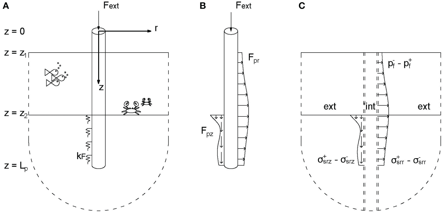
The sub-structuring approach of the model: (A) the model geometry, (B) the in-vacuo pile substructure with an external load on top and distributed loads representing the fluid and soil response, and (C) the internal and external fluid-soil substructures with the pile load acting on the boundaries at r = rp.
The interface conditions between the pile and soil are crucial in the modeling approach. The present model allows for relative motion between pile and soil via a contact stiffness element that varies in stiffness between the ultimate cases of perfect contact (PC), and no friction (NF), i.e. frictionless sliding. The authors believe that introducing the contact stiffness element improves noise prediction without computationally expensive non-linear time-domain calculations because it allows for limited relative motion between pile and soil, which is considered necessary for noise emission modeling. This study considers a frequency- and depth-independent contact spring element, though the element can theoretically contain both spring and damper and can be depth- and frequency-dependent. The idea behind this approach is that the pile is considered around a particular equilibrium state, i.e., the penetration depth is fixed. The contact spring element can be calibrated further based on a driveability model, i.e., (Tsetas et al., 2023b) or experimental data.
2.2 Governing equations
The analysis in this study is performed in the frequency domain, making use of the following Fourier transform pair:
The pile, fluid, and soil domains are referred to by subscript p, f, and s, respectively. Subscripts r and z refer to the radial and the vertical direction, respectively. The equations of motion of the pile read:
where Lp represents the stiffness components of Flügge’s thin shell theory (Leissa, 1973) and depends on the shell material and geometrical properties. contains the displacements of the pile. The hammer force is modeled as a distributed load on top of the pile via , while the fluid and soil reactions are lumped in . The interaction with fluid and soil can be written as a convolution over the length of the pile of the effective dynamic stiffness of the fluid-soil domain and the pile displacements: . is the analytical description of the effective dynamic stiffness, including the contact spring element, coupling the radial and the vertical direction. This convolution is later evaluated numerically and substituted by the boundary element matrix. The fluid and soil media are modeled as acoustic and linearly elastic continua. The equations of motion read:
The fluid equation of motion is written as a function of the displacement potential ϕf (r, z), with and fluid pressure , including as volume injection source at the location of the pile (Jensen et al., 2011). The soil equation of motion contains displacements vector and body forces vector at the radius of the pile. The boundary value problem for the fluid-soil substructure is composed of a single fluid layer overlaying a soil half-space. The accompanying interface conditions read:
Next to the interface conditions, the Sommerfeld radiation condition is applied at the infinite boundaries. Last, the two substructures are coupled via the interface conditions on the pile’s interior and exterior surfaces. The interior surface is indicated with superscript ‘-’ and the exterior with ‘+’. The interface conditions read:
in which is the introduced contact stiffness element that allows for relative motion between pile and soil in the vertical direction. The limit cases of PC and NF are approached by the limits of and , respectively. In all cases, the continuity of displacements in the radial direction and equilibrium of stresses are satisfied.
2.3 Solution method
A solution for the pile and fluid-soil substructure is found independently and coupled via the interface conditions. A summation of in-vacuo modes describes the pile substructure, and an indirect boundary element approach defines the fluid-soil domain. Green’s functions for a layered medium are obtained in the wavenumber domain (Section 3), and retrieved in space by the wavenumber integration technique (Jensen et al., 2011). A boundary element matrix for the interior and exterior fluid-soil domainsis first obtained and subsequently substituted into the interface conditions: Eqs. (9) to (14). From the interface conditions, an effective boundary element matrix is derived based on the pile displacements, which is then substituted back into the equation of motion of the pile. Last, the orthogonality relation of the structural modes is applied to find the complex-valued modal coefficients.
First, the equation of motion of the pile is rewritten:
Then the displacement field of the pile is decomposed into a summation of structural modes, i.e.:
The mode shapes Up,k (z) are found by solving the eigenvalue problem of the in-vacuo pile with free-end boundary conditions. The modal amplitudes are obtained after pre-multiplying Eq. (15) with another mode l once expressed in the modal domain, and subsequently, integrating over the length of the pile:
in which δlk is the Kronecker delta function, and Nk is expressed as:
The boundary element matrix of the fluid-soil substructure is derived based on the indirect boundary element method. The indirect boundary integral for a field ϕ at p and a source σ at q reads (Kirkup, 2019):
with np being the normal vector and the constant when p is on Γq and cp = 0 otherwise. The boundary element matrix is found after substituting Eq. (20) in Eq. (19) and eliminating the sources σ(q). The boundary element matrices for the interior and exterior domains are found based on the same Green’s function, though the normal vector np changes direction. Since the problem is cylindrically symmetric with sources at the pile radius r = rp, Green’s functions are derived for ring sources in both domains. The displacements and stress fields in fluid and soil are expressed in terms of Green’s functions. The displacements, pressure, and stresses are expressed as integrals over all sources on the pile surface.
in which α = r, z, corresponds to the radial and vertical direction. The frequency domain Green's functions and Green’s tensors are given by and , respectively. The superscript and operator ± in Eqs. (21) and (24) corresponds to the exterior (+) and interior (-) domain and originates from the direction of the normal vector np in Eq. (20). Numerical integration of Eqs. (21) to (24) results in a discrete matrix relating displacements, pressure, and stresses to the ring sources, both in the exterior and the interior domain, indicated with ± respectively. Because Green’s functions are singular at the source, it is chosen to have a source of constant amplitude over the height of an element to circumvent the singularity; i.e., the integrals are evaluated by the midpoint rule. Additionally, the integration scheme positively affects the convergence rate of the inverse Hankel transforms addressed later. The Green’s functions and Green’s tensor functions are derived in Section 3.
with I being the identity matrix and the overhead bar indicating that the variables are discretized. After some standard linear algebra, stresses and displacements are related via the dynamic stiffness matrix of the fluid-soil domain:
The effective fluid-soil stiffness matrix in Eq. (17) is a function of the pile displacements and therefore includes the description of the pile-soil interface condition. Thus, the convolution integral is numerically evaluated by substituting Eq. (26) into Eqs. (9) to (14). In the PC case, the effective stiffness fluid-soil matrix is equal to the matrix found in Eq. (26), i.e.,
3 Fluid-soil Green’s functions
The Green’s functions for a layered medium are derived in two steps. First, Green’s functions for the infinite space are derived from a ring source in both fluid and soil media. Second, the infinite space Green’s functions are substituted in the boundary value problem. Since the problem is cylindrically symmetric with sources at r = rp, Green’s functions are derived for ring sources in both domains. First, the soil displacements are decomposed into potentials:
. Hereafter, the problem is transformed to the frequency-wavenumber domain by making use of the following Hankel transform pair:
The fluid-soil domain is split into an interior and an exterior domain at the position of the pile, r = rp. The applied indirect boundary method includes Green’s functions of ring sources at the pile’s location and derives the displacement and stress field at the boundary as a function of the sources. The potential solution is sought for in the form of a homogeneous solution and a particular solution:
The particular solutions in Eqs. (28) to (30) are derived from the infinite space Green’s functions introduced in Sections 3.1 and 3.2. The homogeneous part is based on the boundary value problem, given by Eqs. (5) to (8). The problem is transformed to the wavenumber domain by applying Eq. (27):
which can be expressed in potentials via:
The Green’s functions and Green’s tensors in Eqs. (21) to (24) are found by substituting the potential in the displacements and stresses and by applying the inverse Hankel transform.
3.1 Fluid source
The ring source in the fluid is introduced in the form of a ring volume injection , of which the wavenumber counterpart is designated as . Equation (3) is transformed to the wavenumber domain by applying Eq. (27) to give:
with and zs the source position. The infinite space Greens function for a ring load in the wavenumber domain is given by Peng et al. (2021a):
The Green’s functions for a layered medium are obtained after substituting the free field particular solution given by Eq. (40) into Eq. (28) and the boundary value problem: Eqs. (31) to (34), and applying the inverse Hankel transform.
3.2 Soil source
Similarly to the fluid source, a distributed ring load at r = rp excites the infinite space. The force is directed either in the radial or the vertical direction. Equation (4) is first transformed to the wavenumber domain resulting in the following coupled equations:
with , , , and . The potentials for a ring load in the radial direction in an infinite elastic space read:
Similarly, the potentials for a vertical load read:
Again, the displacement and stress field at boundary r = rp are found in terms of Green’s functions and Green’s tensor functions by substitution of the particular solutions in the boundary value problem.
4 Model verification
The model developed in this paper is verified against a finite element model in ‘COMSOL Multiphysics®’ (COMSOL, 2019), with input data from the COMPILE benchmark case (Lippert et al., 2016), together with the near-field responses in the companion paper (Lippert et al., 2016). In the COMPILE case, the soil domain is represented by an acoustic fluid though. Therefore, soil parameters are adapted from Peng et al. (2021a) to validate the elastic soil case, and all properties are summarized in Table 1. The verification is performed under perfect contact conditions in which no sliding is allowed between the pile and the soil.
Table 1
| Parameter | unit | Parameter | unit | ||
|---|---|---|---|---|---|
| Sea surface depth [z1] | 0 | m | Structural damping | 0.001 | - |
| Seabed depth [z2] | 10 | m | Fluid wavespeed [cf] | 1500 | m s−1 |
| Final penetration depth | 25 | m | Fluid density [ρf] | 1025 | kg m−3 |
| Pile length [Lp] | 25 | m | Compression wavespeed soil [cL] | 1800 | m s−1 |
| Pile thickness [tp] | 0.05 | m | Shear wavespeed soil [cT] | 170 | m s−1 |
| Pile radius [rp] | 1 | m | Soil density [ρs] | 2000 | kg m−3 |
| Pile Poisons ratio [vp] | 0.30 | - | Compressional wave attenuation [αL] | 0.469 | dB/λ |
| Pile Youngs modulus [Ep] | 210 | GPa | Shear wave attenuation [αT] | 1.69 | dB/λ |
| Pile density [ρp] | 7850 | kg m−3 |
Model properties for model verification in Section 4.
Parameters adapted from Lippert et al. (2016) and Peng et al. (2021a).
For the validation of the near field model, a harmonic load on top of the pile is considered at frequencies up to 500 Hz. Boundary elements of 0.05 m are used; the mesh is sufficiently small compared to the shortest wavelength of 0.34 m. The upper limit in the inverse Hankel transform is fixed at k = 500 m-1 which is sufficiently large because it guarantees that all integrands are smaller than 0.2% of the maximum amplitude. The truncation might seem unnecessarily high compared to the Scholte wavenumber at f = 500 Hz, i.e., kscholte ≈ 20.5 m–1, however, it is deemed necessary when source and receiver are positioned at close distance. Pile, fluid, and soil transfer functions are validated for a load amplitude of 1 MN on top of the pile throughout the frequency range. Figure 2 shows the pile displacements at three frequencies distributed within the frequency domain of interest for vibratory pile driving (∼15 → 500 Hz). The pile displacements predicted by Comsol and the present model are in excellent agreement.
Figure 2
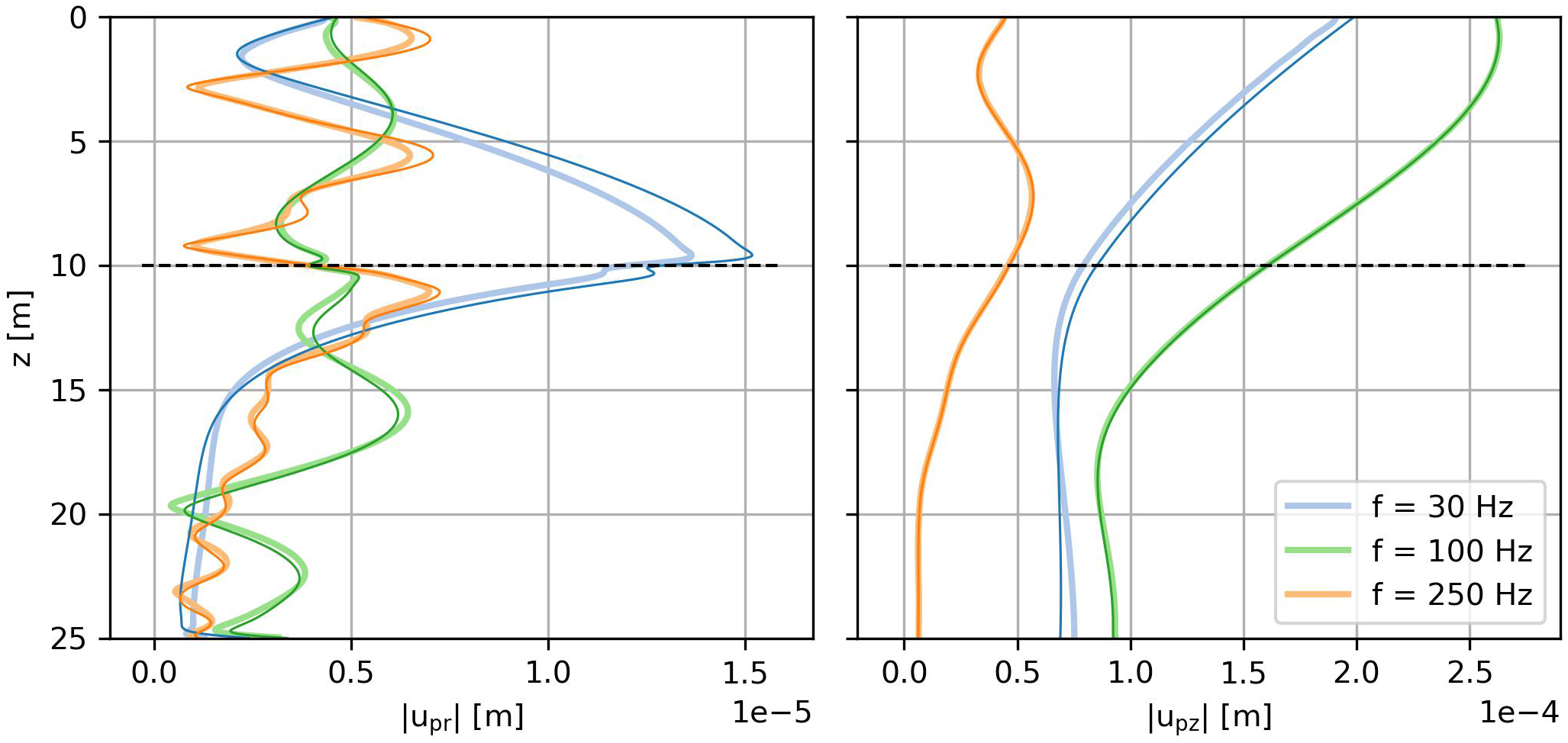
Comparison of the amplitudes of the pile vibrations between Comsol (dark colors) and the present model (light colors) for a harmonic load of 1 MN on top of the pile at 30, 100 and 250 Hz.
The sound pressure level (Lp) in the fluid is calculated by (ISO, 2017):
in which the real mean square in the frequency domain is found by and the reference pressure in underwater acoustics is pref = 1µPa. The sound pressure levels in the near field are in excellent agreement between Comsol and the present model, both in the center of the fluid layer (z = 5 m) and at one meter above the seabed surface (z = 9 m) as shown in Figure 3.
Figure 3
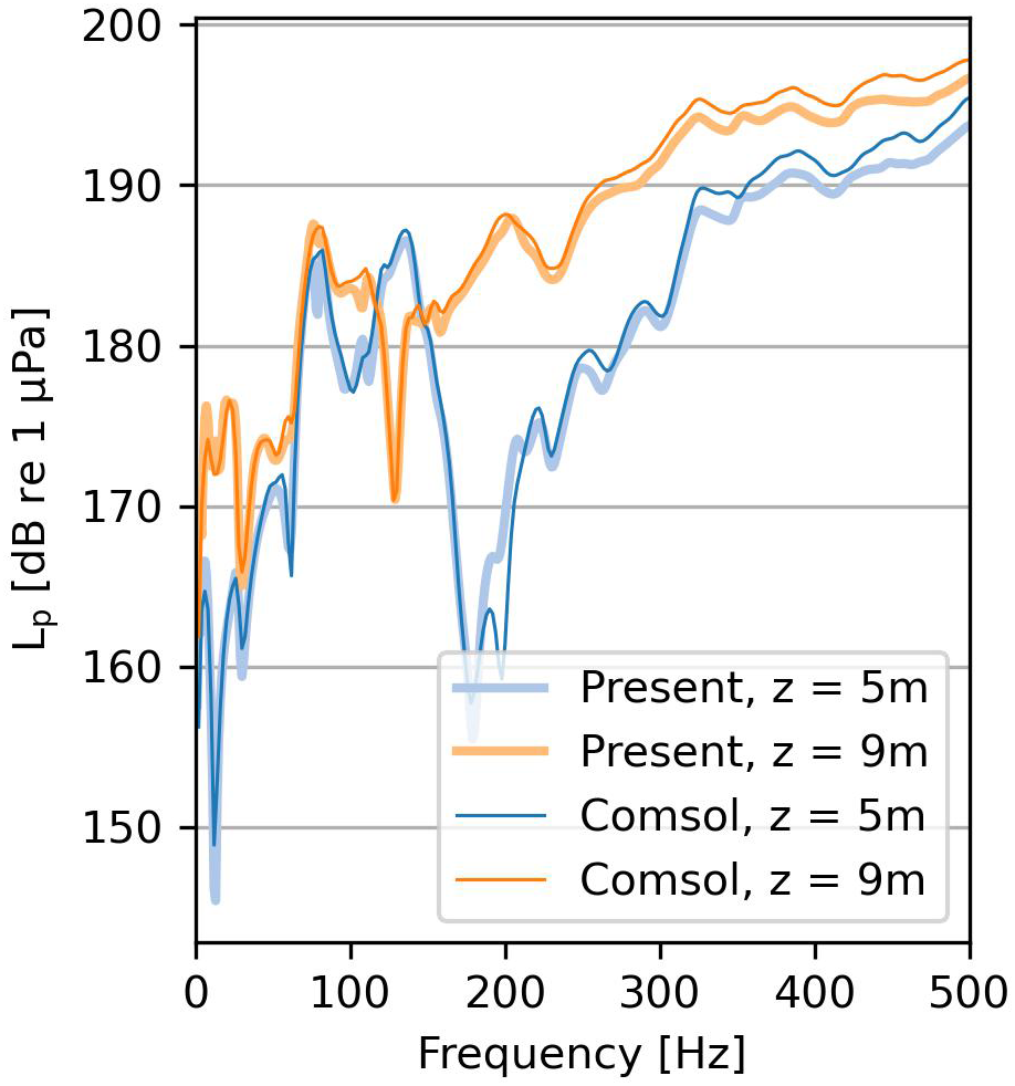
Comparison of the sound pressure levels in the water at a radius of 10 m between Comsol (dark colors) and the present model (light colors) for a harmonic load of 1 MN.
5 Effect of pile-soil interface conditions
A realistic case study is considered hereafter to examine the effect of varying pile-soil interface conditions based on the geometry and material parameters described in Dahl et al. (2015) and measurements of a representative vibratory force by Tsetas et al. (2023a). The data can be used together since both campaigns used piles with an equal diameter of 0.762 m and comparable driving depths into the soil. Table 2 includes all parameters used in the case study.
Table 2
| Parameter | unit | Parameter | unit | ||
|---|---|---|---|---|---|
| Sea surface depth [z1] | 1.4 | m | Structural damping | 0.001 | - |
| Seabed depth [z2] | 8.9 | m | Fluid wavespeed [cf] | 1475 | m s−1 |
| Final penetration depth | 16 | m | Fluid density [ρf] | 1000 | kg m−3 |
| Pile length [Lp] | 17.4 | m | Compression wavespeed soil [cL] | 1850 | m s−1 |
| Pile thickness [tp] | 2.54 | m | Shear wavespeed soil [cT] | 400 | m s−1 |
| Pile radius [rp] | 0.762 | m | Soil density [ρs] | 1900 | kg m−3 |
| Pile Poisons ratio [vp] | 0.28 | - | Compressional wave attenuation [αL] | 0.03 | dB/λ |
| Pile Youngs modulus [Ep] | 210 | GPa | Shear wave attenuation [αT] | 0.20 | dB/λ |
| Pile density [ρp] | 7850 | kg m−3 |
Model properties used to examine the effect of pile-soil interface conditions based on parameters in Section 5.
Parameters adapted from Dahl et al. (2015).
The applied force at the top of the pile is derived from actual strain measurements as shown in Figure 4. The force is periodic and consists of a primary driving frequency of 25 Hz and strong super-harmonics every 25 Hz. The super-harmonics play a major role in noise emission because at these frequencies sound radiation is more efficient than the main driving frequency. This is confirmed by Dahl et al. (2015) (Figure 3), where the measured sound pressure levels at the super-harmonics are of higher amplitude than the sound pressure level at the main driving frequency.
Figure 4
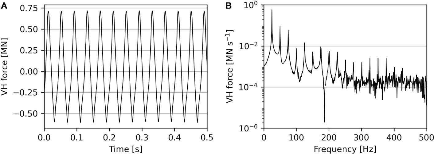
Estimated vibratory force exerted by the installation tool at the pile head as a function. (A) shows the time signature and (B) the amplitude spectrum of the force (Tsetas et al., 2023a).
The Scholte wave often plays a significant role in underwater noise at relatively low frequencies. The intensity of this wave is often overestimated if the pile and soil are assumed in perfect contact. Hereafter, relative motion is allowed between pile and soil via a linear spring element introduced at the pile-soil interface. Four cases are evaluated; a case with perfect contact between pile and soil (PC), a case of no frictional forces (NF), and two cases with relaxed pile-soil contact via the interface element. The interface element relaxes the static (f = 0 Hz) vertical soil stiffness to 75% and 5% of its original stiffness. The cases are abbreviated to kF 75% and kF 5%, and correspond to values of and , respectively.
5.1 Pile vibrations
Allowing for relative motion between pile and soil affects the pile vibrations and the energy transferred to the surrounding domain. Figure 5 shows the amplitude of the pile displacements at 25 Hz and 125 Hz for varying values of . The frequencies are chosen specifically at the driving frequency and the fourth super-harmonic. Figure 5A shows that the rigid body motion governs the pile vibrations at low frequencies. For kF 5%, the radial pile and soil displacements are amplified. This is counterintuitive, but because the system has reduced soil stiffness and low damping, the resonance amplitude of the rigid body mode is amplified significantly. At higher frequencies, the dynamic response of the pile is strongly influenced by the pile-soil interface as shown in Figure 5B; altering the noise source significantly in the fluid domain.
Figure 5
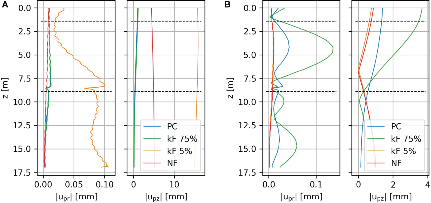
The amplitudes of the pile displacements in radial (upr) and vertical (upz) direction for a 1 MN harmonic force on top of the pile at 25 Hz and 125 Hz in (A, B), respectively.
5.2 Underwater noise field and seabed vibrations
The change in pile dynamics affects the soil displacements and pressure levels in the fluid. The traveling waves in fluid and soil are visualized in Figure 6. The figure shows snapshots of the fluid pressure and vertical soil displacement in the surroundings. Figure 6A shows that the Scholte waves govern the wavefield because the excitation frequency is below the cut-off frequency of this shallow fluid waveguide (fcut-off ≈ 37.5 Hz). The cut-off frequency linearly depends on water depth; thus, a pressure wave can exist at the driving frequency in the case of deeper waters. The Scholte wave is visible in the soil and fluid, though the amplitude is negligible in case of perfect sliding conditions (NF case). The soil motion is amplified at kF 5% because the main driving frequency is close to the eigenfrequency of the rigid body mode. It is debatable if this resonance is an artifact or physical. Experimental data should justify if it is indeed physical or that the artifact disappears with more realistic interface modeling, e.g. including damping. Contrary, Figure 6B clearly shows bulk pressure waves propagating through the fluid, while the Scholte waves influence a narrow zone close to the seabed. Next, the Scholte wave becomes visible with increasing pile-soil stiffness, though the penetration zone in the fluid reduces at higher frequencies due to the shorter wavelength of the Scholte waves. Figure 6 confirms the expectation that the interface conditions strongly affect both primary and secondary noise paths.
Figure 6
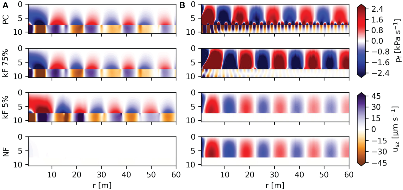
(A, B) show the real part of the fluid pressure and vertical soil displacement for a harmonic 1 MN force at 25 Hz and 125 Hz respectively.
Figure 7 shows the sound pressure levels as a function of range and depth for varying cases. The pressure levels are highest above the seabed both from the primary and secondary noise path and decay with distance. With increasing contact stiffness kF, the interference of pressure waves in the fluid and Scholte waves is clearly visible in Figure 7B. Negligible noise is generated in the case of NF at 25 Hz because this frequency is below the cut-off frequency of propagating body modes in the fluid and almost no energy is transferred to the Scholte waves due to the lack of shear excitation.
Figure 7
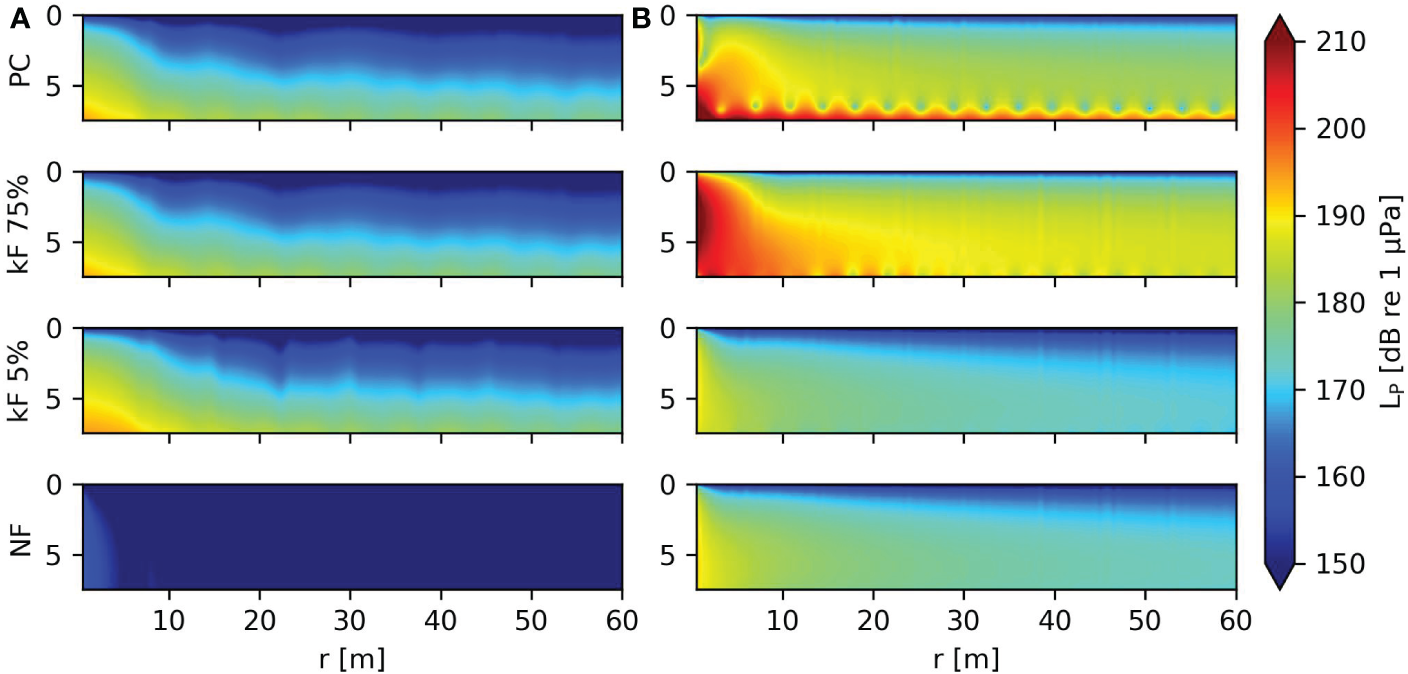
Figure (A, B) show the sound pressure levels in dB versus depth and height in the fluid for a harmonic 1 MN force at 25 Hz and 125 Hz respectively.
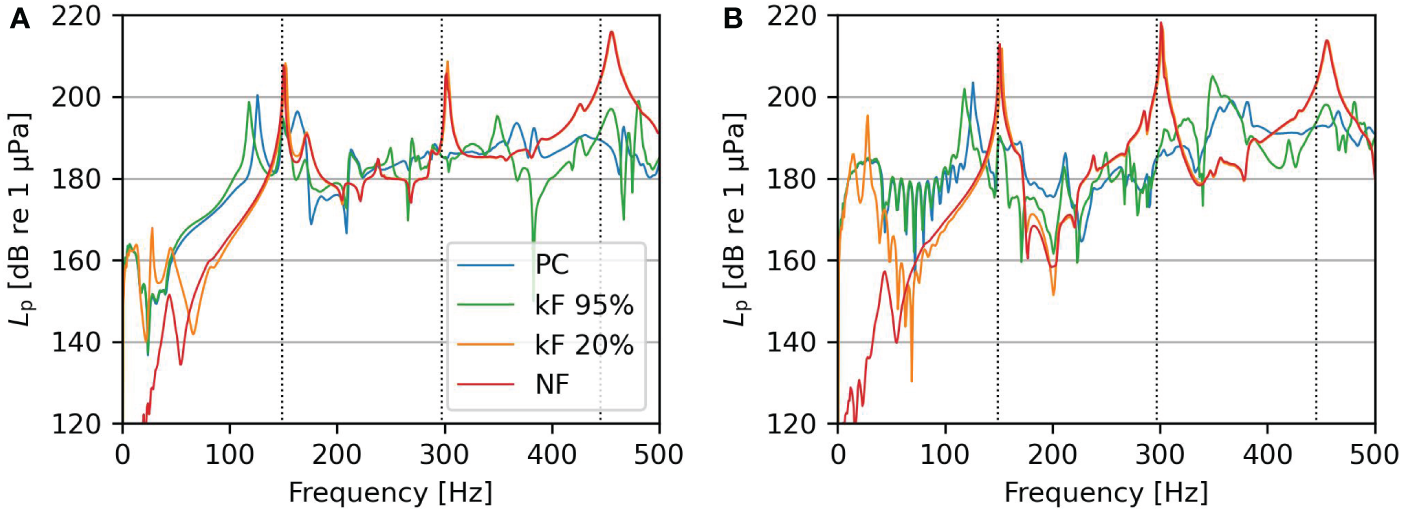
The transfer functions or frequency response functions for a unit 1 MN harmonic load on top of the pile at a receiver point at a radius of 20 m are shown in Figures 8A, B. The sound pressure level transfer functions depend strongly on the contact stiffness element. The sound pressure levels are significantly higher at 0.5 m above the seabed than in the middle of the fluid column for cases with Scholte waves. Scholte waves are most dominant at low frequencies (<200 Hz). At approximately 150, 300, and 450 Hz, the first in-vacuo eigenfrequencies of the pile are indicated with a black dotted vertical line. The sound pressure level amplifies around these frequencies if soil and pile are loosely coupled and the system experiences low damping. Thus, eigenfrequencies play an increasingly important role in the case of reduced resistance. The resonance of the rigid body mode, as discussed in Section 5.1, is visible at 23 Hz for kF 5%. It is debatable whether this mode is physical or not. One might say that, in reality, this mode can exist at low frequencies with reduced soil resistance. On the other hand, it can be argued that frictional damping limits this resonance behavior. Damping at the pile-soil surface via an imaginary part in kF can represent the interface damping.
Figure 8
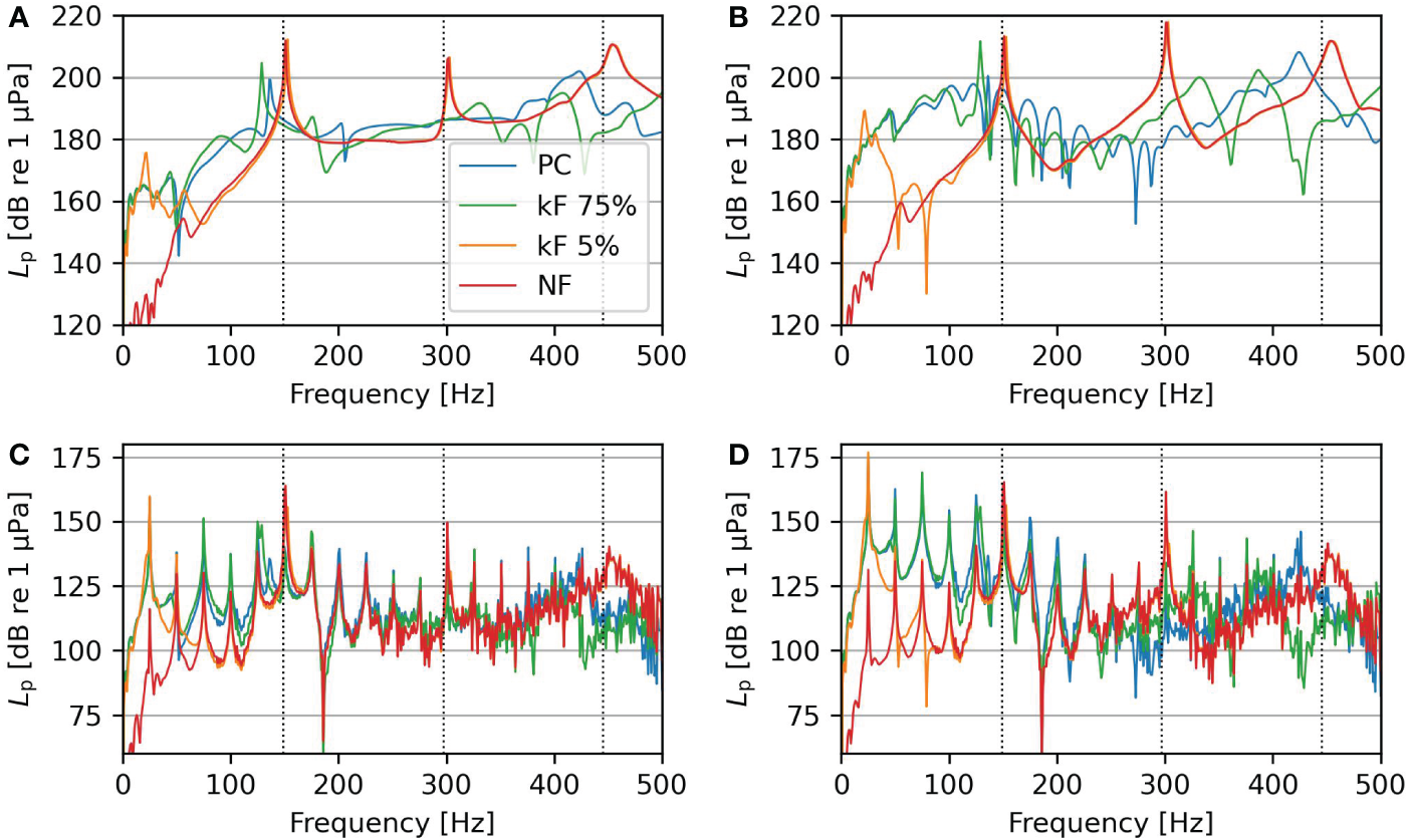
(A, B) show the sound pressure level transfer functions for a 1 MN harmonic load on top of the pile at a 20 m radius and z = 3 m and z = 7 m, respectively. (C, D) show the sound pressure levels resulting from the vibratory force from Figure 4 at a 20 m radius and z = 3 m and z = 7 m, respectively. The dotted vertical lines indicate the eigenfrequencies of the pile.
The importance of the sound pressure level transfer functions becomes evident when the actual force is applied at the top of the pile by multiplying the transfer functions with the spectrum of the force plotted in Figure 4B. Figures 8C, D shows the periodicity of the peaks related to the force spectrum. The surface waves at low frequencies govern the noise field above the seabed except for the NF case as shown in Figure 8D. In the middle of the fluid layer, the peaks are of similar amplitude for most super-harmonics. In the case of NF and kF 5%, the in-vacuo eigenfrequencies of the pile amplify the sound pressure level next to the peaks enforced by the external force.
Applying the inverse Fourier transform gives the periodic time domain response of the fluid and soil. Figure 9 shows a snapshot of the time domain pressure field in the fluid and vertical displacements in the soil. The Scholte waves at the driving frequency govern the wavefield in all cases except for the case of NF. In the upper part of the fluid layer, interference patterns are visible in fluid pressure waves of varying wavelengths. The predominant pressure wave pattern in the case of NF corresponds to a frequency of approximately 150 Hz i.e., the first eigenfrequency of the pile, in line with expectations from the earlier analysis.
Figure 9
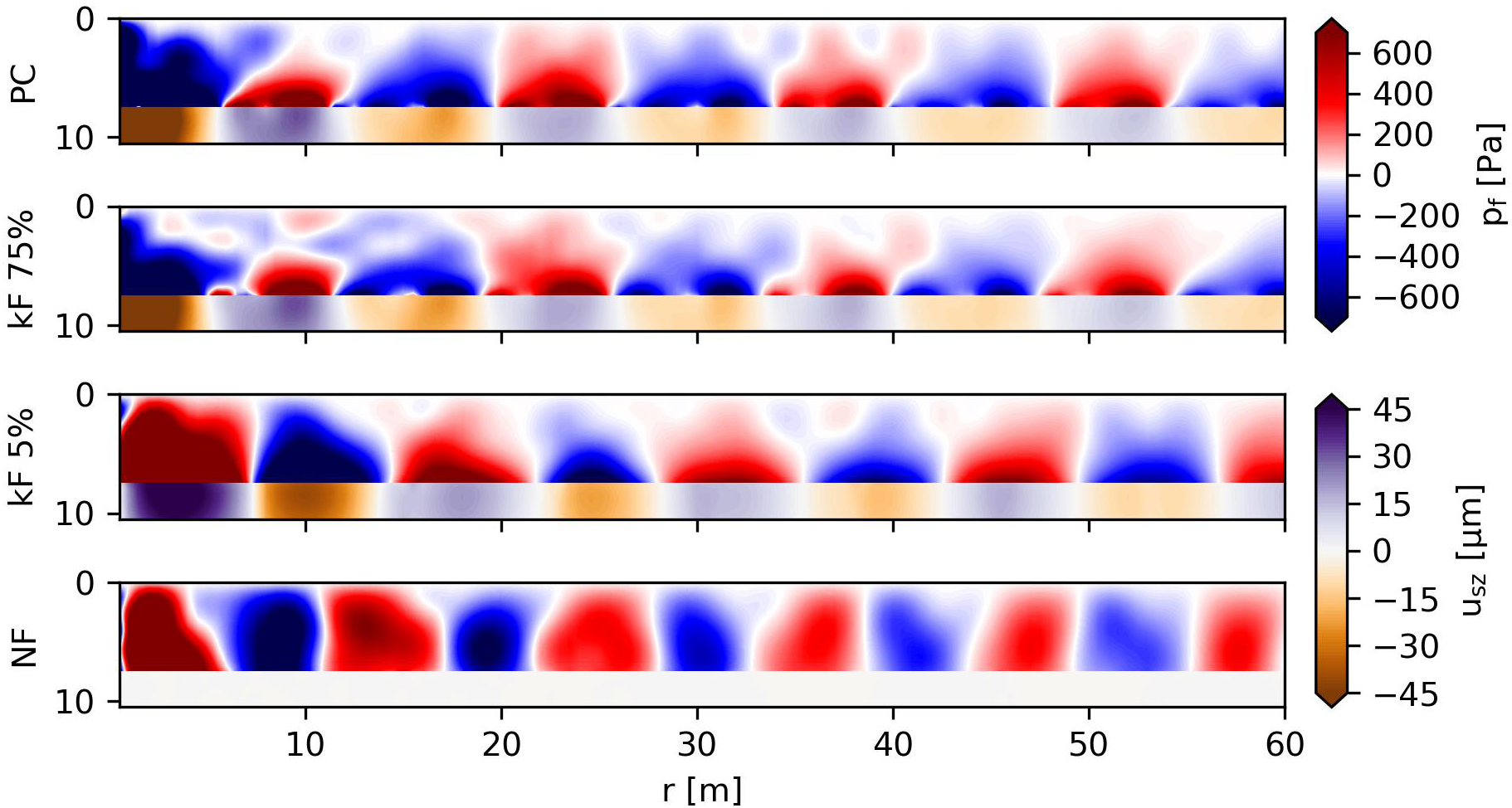
Snapshot of the time domain pressure field for the periodic force for varying interface conditions.
To examine the accumulative noise pollution over a time interval, the sound exposure levels (LE) are calculated. The sound exposure level shows the time-integrated squared sound pressure in decibels and are calculated via (ISO, 2017):
with the reference value for sound pressure in fluids Eref = 1μ Pa2s. Figure 10 shows the sound exposure levels in the fluid domain throughout 1 second of the forced response. The amplitude of the sound exposure levels varies strongly with the various cases with no particular trend. In the NF case, the sound exposure is governed by the bulk pressure waves, while in the PC case, the Scholte waves contribute significantly. This shows that the sound exposure level above the seabed is highest in the Scholte waves’ presence. In the case of NF, the bulk pressure wave causes lower sound exposure levels above the seabed but relatively higher levels in the middle and upper part of the fluid column.
Figure 10
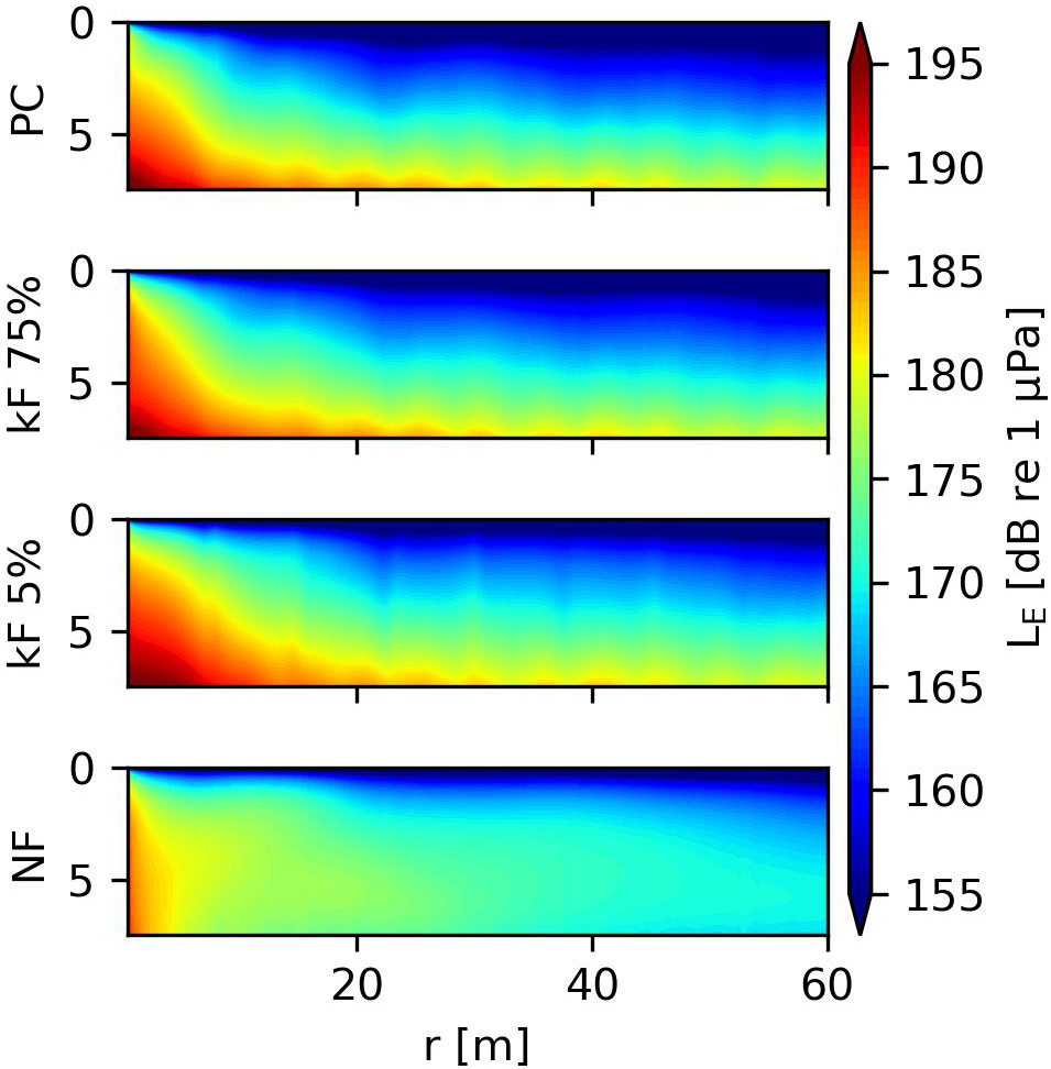
Sound exposure levels in dB versus depth and height in the fluid throughout 1 second forcing.
Biologists are additionally interested in particle velocity of fluid and seabed for environmental assessment. Figure 11 shows the particle velocity norm and directionality at a snapshot in time. The figure shows that the predominant particle motion is along the vertical direction at the seabed-water interface. However, in the absence of the Scholte waves, the particle motion direction is governed by the radial direction due to the bulk pressure waves alone.
Figure 11
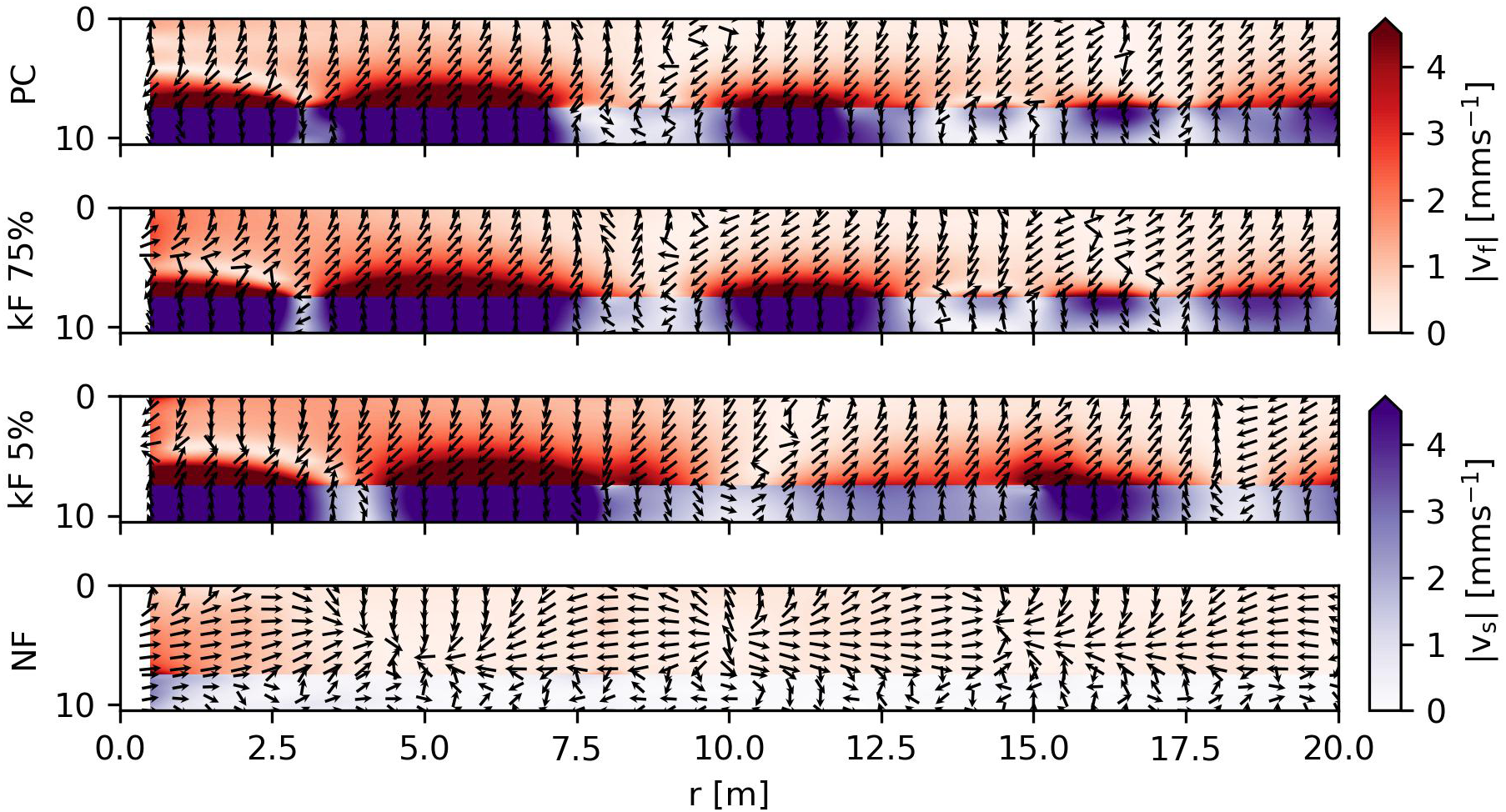
Snapshot of particle velocity norm in mm s–1 in fluid and soil domains including velocity directionality.
5.3 Reduced soil shear stiffness
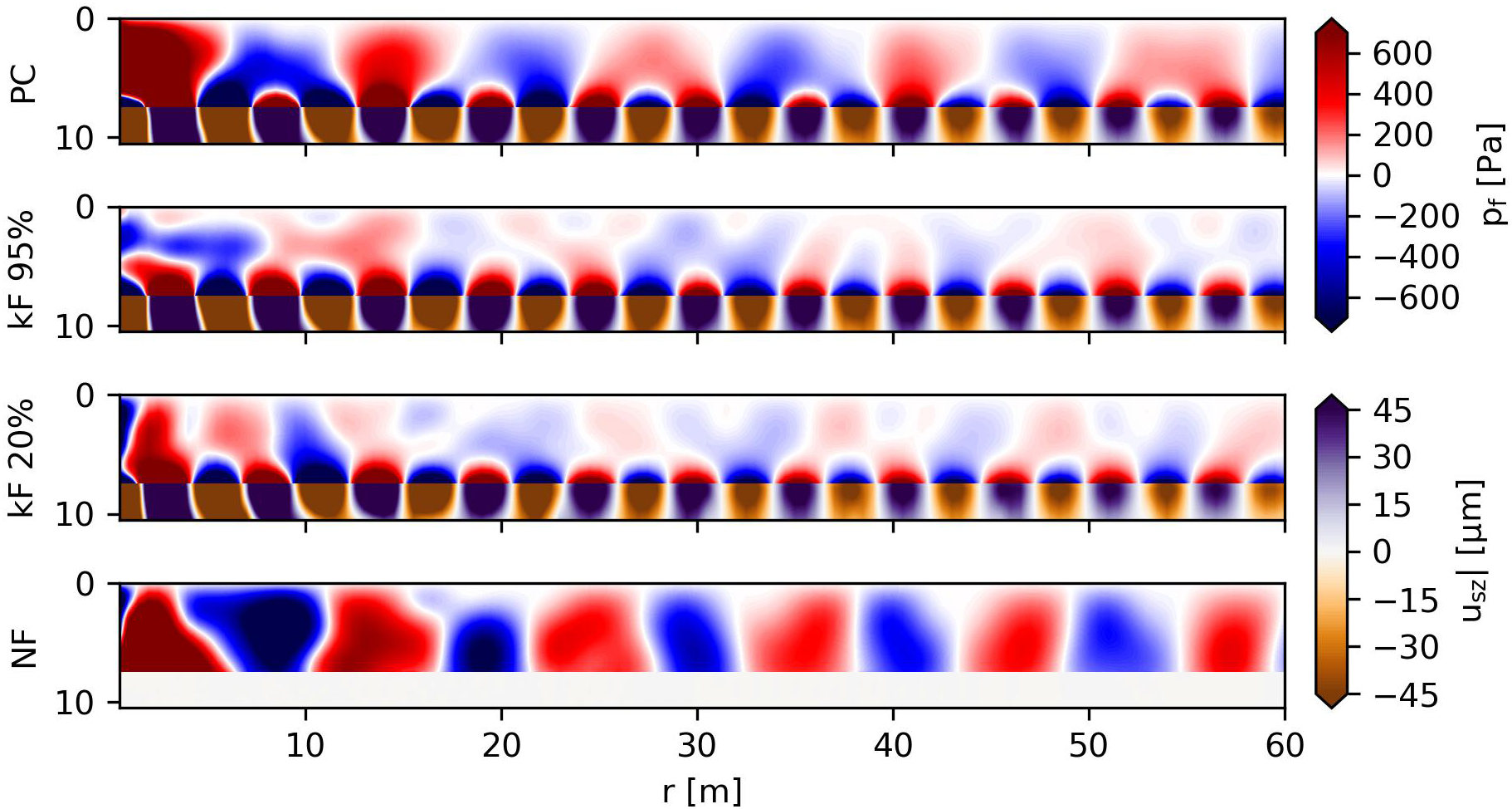
The experimental campaign in Dahl et al. (2015) consists of soil with high shear wave speed. In many known cases, the shear wave speed is significantly lower. Since the shear wave speed strongly influences the amplification of the Scholte waves, the analysis is repeated for a reduced shear wave speed of 150 ms–1, which is typical in marine environments with sandy sediments in the North Sea in Europe (Peng et al., 2021a). The rest of the parameters are given in Table 2. This results in a relative reduction of the stiffness to 95% and 20% compared to the static stiffness for the rigid body mode, for a contact spring element kF of 5 × 10⁸ N m–1 and 5 × 10⁶ N m–1, respectively.
Figure 12 shows the transfer functions of the pressure field, similarly to Figures 8A, B. Both figures show similar behavior, though the differences in pressure levels between the cases in sound pressure levels are smaller with lower shear wave speed at frequencies between 100 Hz and 350 Hz.
Figure 12
(A, B) show the sound pressure level transfer functions for a 1 MN harmonic load on top of the pile at 20 m radius and soil with a low shear modulus.
Figure 13 shows a snapshot of the time domain fluid pressures and the vertical soil displacements. The Scholte waves visible differ significantly compared to Figure 9. The Scholte wave is of a shorter wavelength due to the lower shear wave speed and has a reduced penetration into the fluid zone. Thus, the primary noise path becomes more pronounced. The reduced penetration of the Scholte waves also explains the reason why the Scholte waves contribute less to the sound pressure levels in Figure 12 compared to the case shown earlier. Contrary, the vertical displacements in the soil are of larger amplitude compared to Figure 9. Otherwise, the principles of noise generation align with the original case. Even for soil with lower shear wave speeds, the role of the interface waves in the noise generation remains significant, causing dominant pressure levels and seabed vibrations.
Figure 13
Snapshot of time domain pressure field for the periodic force for varying interface conditions with soil with a low shear modulus.
6 Conclusion
This paper concludes that models for impact pile driving are not directly applicable in vibratory pile driving because a more advanced description of pile-soil interaction is essential for predicting noise and vibrations accurately. The pile-soil interface condition strongly influences the dynamic response of the pile and the energy transfer mechanism in the surrounding domain. More specifically:
-
The dynamic response of the pile depends strongly on the coupling to the soil, which, in turn, influences the primary noise and secondary noise paths.
-
In case pile and soil are loosely coupled, the in-vacuo eigenfrequencies of the pile play an increasingly important role in noise generation. The reduced damping and stiffness in the system cause amplification of the structural vibrations around the eigenfrequencies of the coupled system.
-
In the case of strong pile-soil coupling, Scholte interface waves are amplified and contribute significantly to the fluid pressures. The Scholte waves govern the seabed vibrations for high and low shear speeds. Due to the possible intense seabed vibrations, marine life on or above can potentially be harmed. The Scholte waves are significant at low frequencies and, therefore, more important in vibratory installation compared to impact pile driving.
-
The pile-soil interface conditions strongly influence the particle velocity field.
Even with a relaxation of the pile-soil interface condition, the presence of the Scholte wave affects the sound field due to the relatively low primary excitation frequency. Therefore, models representing the soil by an acoustic fluid are insufficient invibratory pile driving. This study shows the noise generation mechanisms qualitatively in the case of piles installed with vibratory tools. Future research in describing the interface condition and experimental data to validate the model is needed for a fully quantitative investigation.
Statements
Data availability statement
The original contributions presented in the study are included in the article/supplementary material. Further inquiries can be directed to the corresponding author.
Author contributions
TM, AT, and AM contributed to the concept of the study. TM built the model and ran the analysis. AT and AM gave important feedback on the results, and all discussed the interpretation of the results. TM wrote the first draft of the manuscript; AT significantly directed the manuscript’s content. All authors contributed to the manuscript revision and read and approved the submitted version.
Funding
This research is funded in the framework of the Grow joint research program by “Topsector Energiesubsidie van het Ministerie van Economische Zaken” under grant number TE-HE117100.
Acknowledgments
This research is associated with the GDP project in the framework of the GROW joint research program. Funding from “Topsector Energiesubsidie van het Ministerie van Economische Zaken” under grant number TE-HE117100 and financial/technical support from the following partners is gratefully acknowledged: Royal Boskalis Westminster N.V., CAPE Holland B.V., Deltares, Delft Offshore Turbine B.V., Delft University of Technology, ECN, EnecoWind B.V., IHC IQIP B.V., SHL Offshore Contractors B.V., Shell Global Solutions International B.V., Sif Netherlands B.V., TNO, and Van Oord OffshoreWind Projects B.V.
Conflict of interest
The authors declare that the research was conducted in the absence of any commercial or financial relationships that could be construed as a potential conflict of interest.
Publisher’s note
All claims expressed in this article are solely those of the authors and do not necessarily represent those of their affiliated organizations, or those of the publisher, the editors and the reviewers. Any product that may be evaluated in this article, or claim that may be made by its manufacturer, is not guaranteed or endorsed by the publisher.
References
1
Benhemma-Le Gall A. Graham I. M. Merchant N. D. Thompson P. M. (2021). Broad-scale responses of harbor porpoises to pile-driving and vessel activities during offshore windfarm construction. Front. Mar. Sci.8. doi: 10.3389/fmars.2021.664724
2
COMSOL (2019). Comsol multiphysics® v. 5.6 (stockholm, sweden: comsol ab). Available at: www.comsol.com.
3
Cui C. Meng K. Xu C. Wang B. Xin Y. (2022). Vertical vibration of a floating pile considering the incomplete bonding effect of the pile-soil interface. Comput. Geotechnics150, 104894. doi: 10.1016/j.compgeo.2022.104894
4
Dahl P. H. Dall’Osto D. R. Farrell D. M. (2015). The underwater sound field from vibratory pile driving. J. Acoustical Soc. America137, 3544–3554. doi: 10.1121/1.4921288
5
European Commission (2020). Communication from the commission to the European parliament, the council, the European economic and social committee and the committee of the regions: An EU strategy to harness the potential of offshore renewable energy for a climate neutral future (Brussels, Belgium: Tech. rep).
6
Fernandez-Betelu O. Graham I. M. Brookes K. L. Cheney B. J. Barton T. R. Thompson P. M. (2021). Far-field effects of impulsive noise on coastal bottlenose dolphins. Front. Mar. Sci.8. doi: 10.3389/fmars.2021.664230
7
Fricke M. B. Rolfes R. (2015). Towards a complete physically based forecast model for underwater noise related to impact pile driving. J. Acoustical Soc. America137, 1564–1575. doi: 10.1121/1.4908241
8
Heitmann K. Mallapur S. Lippert T. Ruhnau M. Lippert S. von Estorff O. (2015). Numerical determination of equivalent damping parameters for a finite element model to predict the underwater noise due to offshore pile driving. Euronoise2015, 605–610.
9
Holeyman A. E. (2002). Soil behaviour under vibratory driving. Proceedings of the International Conference on Vibratory Pile Driving and Deep Soil Compaction, Transvib 2002. 3–20.
10
ISO . (2017). ISO 18405:2017 underwater acoustics — terminology (Geneva, Switzerland).
11
Jensen F. B. Kuperman W. A. Porter M. B. Schmidt H. (2011). Computational ocean acoustics. 2nd ed. (New York, NY: Springer New York). doi: 10.1007/978-1-4419-8678-8
12
Kirkup S. (2019). The boundary element method in acoustics: A survey. Appl. Sci. (Switzerland)9, 1642. doi: 10.3390/app9081642
13
Leissa A. W. (1973). Vibration of shells (Washington, D.C: Tech. rep., Scientific and Technical Information Office National Aeronautics and Space Administration).
14
Lippert S. Nijhof M. Lippert T. Wilkes D. Gavrilov A. Heitmann K. et al . (2016). COMPILE–a generic benchmark case for predictions of marine pile-driving noise. IEEE J. Oceanic Eng.41, 1061–1071. doi: 10.1109/JOE.2016.2524738
15
Lippert T. von Estorff O. (2014a). On a hybrid model for the prediction of pile driving noise from offshore wind farms. Acta Acustica united Acustica100, 244–253. doi: 10.3813/AAA.918717
16
Lippert T. von Estorff O. (2014b). The significance of parameter uncertainties for the prediction of offshore pile driving noise. J. Acoustical Soc. America136, 2463–2471. doi: 10.1121/1.4896458
17
MacGillivray A. O. (2013). A model for underwater sound levels generated by marine impact pile driving. J. Acoustical Soc. America134, 4024–4024. doi: 10.1121/1.4830689
18
Madsen P. Wahlberg M. Tougaard J. Lucke K. Tyack P. (2006). Wind turbine underwater noise and marine mammals: Implications of current knowledge and data needs. Mar. Ecol. Prog. Ser.309, 279–295. doi: 10.3354/meps309279
19
Markou A. A. Kaynia A. M. (2018). Nonlinear soil-pile interaction for offshore wind turbines. Wind Energy21, 558–574. doi: 10.1002/we.2178
20
Nogami T. Konagai K. (1987). Dynamic response of vertically loaded nonlinear pile foundations. J. Geotechnical Eng.113, 147–160. doi: 10.1061/(ASCE)0733-9410(1987)113:2(147
21
Novak M. (1991). “Piles under dynamic loads,” in Second International Conference on Recent Advances In Geotechnical Earthquake Engineering and Soil Dynamics, Vol. 2. 2433–2456. Saint Louis, United States.
22
Peng Y. Tsouvalas A. Stampoultzoglou T. Metrikine A. (2021a). A fast computational model for near- and far-field noise prediction due to offshore pile driving. J. Acoustical Soc. America (Saint Louis, United States) 149, 1772–1790. doi: 10.1121/10.0003752
23
Peng Y. Tsouvalas A. Stampoultzoglou T. Metrikine A. (2021b). Study of the sound escape with the use of an air bubble curtain in offshore pile driving. J. Mar. Sci. Eng.9, 232. doi: 10.3390/jmse9020232
24
Reinhall P. G. Dahl P. H. (2011a). An investigation of underwater sound propagation from pile driving. Tech. Rep.
25
Reinhall P. G. Dahl P. H. (2011b). Underwater Mach wave radiation from impact pile driving: Theory and observation. J. Acoustical Soc. America130, 1209–1216. doi: 10.1121/1.3614540
26
Schecklman S. Laws N. Zurk L. M. Siderius M. (2015). A computational method to predict and study underwater noise due to pile driving. J. Acoustical Soc. America138, 258–266. doi: 10.1121/1.4922333
27
Southall B. L. Finneran J. J. Reichmuth C. Nachtigall P. E. Ketten D. R. Bowles A. E. et al . (2019). Marine mammal noise exposure criteria: Updated scientific recommendations for residual hearing effects. Aquat. Mammals45, 125–232. doi: 10.1578/AM.45.2.2019.125
28
Tsetas A. Tsouvalas A. Gómez S. S. Pisanò F. Kementzetzidis E. Molenkamp T. et al . (2023a). Gentle driving of piles (GDP) at a sandy site combining axial and torsional vibrations: Part I - installation tests. Ocean Eng.270, 113453. doi: 10.1016/j.oceaneng.2022.113453
29
Tsetas A. Tsouvalas A. Metrikine A. V. (2023b). A non-linear three-dimensional pile-soil model for vibratory pile installation in layered media. Int. J. Solids Structures (Under review).
30
Tsouvalas A. (2020). Underwater noise emission due to offshore pile installation: A review. Energies13, 3037. doi: 10.3390/en13123037
31
Tsouvalas A. Metrikine A. V. (2014). A three-dimensional semi-analytical model for the prediction of underwater noise generated by offshore pile driving. J. Sound Vibrationn333, 259–264. doi: 10.1007/978-3-642-40371-2_38
32
Tsouvalas A. Metrikine A. V. (2016). Structure-borne wave radiation by impact and vibratory piling in offshore installations: From sound prediction to auditory damage. J. Mar. Sci. Eng.4, 44. doi: 10.3390/jmse4030044
33
Wood M. A. (2016). Modelling and prediction of acoustic disturbances from off-shore piling (Southampton, United Kingdom: Phd thesis, University of Southampton).
34
Wood M. A. Humphrey V. F. (2013). “Modelling of offshore impact piling acoustics by use of wave equation analysis,” in 1st Underwater Acoustics Conference, Corfu, Greece. 171–178.
35
Zampolli M. Nijhof M. J. J. de Jong C. A. F. Ainslie M. A. Jansen E. H. W. Quesson B. A. J. (2013). Validation of finite element computations for the quantitative prediction of underwater noise from impact pile driving. J. Acoustical Soc. America133, 72–81. doi: 10.1121/1.4768886
Summary
Keywords
underwater noise, offshore pile driving, vibratory pile driving, soil-structure interaction, particle motion, seabed vibrations
Citation
Molenkamp T, Tsouvalas A and Metrikine A (2023) The influence of contact relaxation on underwater noise emission and seabed vibrations due to offshore vibratory pile installation. Front. Mar. Sci. 10:1118286. doi: 10.3389/fmars.2023.1118286
Received
07 December 2022
Accepted
16 February 2023
Published
27 March 2023
Volume
10 - 2023
Edited by
Yuxing Li, Xi’an University of Technology, China
Reviewed by
Ying Jiang, First Institute of Oceanography, China; Zhongchang Song, Xiamen University, China
Updates
Copyright
© 2023 Molenkamp, Tsouvalas and Metrikine.
This is an open-access article distributed under the terms of the Creative Commons Attribution License (CC BY). The use, distribution or reproduction in other forums is permitted, provided the original author(s) and the copyright owner(s) are credited and that the original publication in this journal is cited, in accordance with accepted academic practice. No use, distribution or reproduction is permitted which does not comply with these terms.
*Correspondence: Timo Molenkamp, t.molenkamp@tudelft.nl
This article was submitted to Ocean Observation, a section of the journal Frontiers in Marine Science
Disclaimer
All claims expressed in this article are solely those of the authors and do not necessarily represent those of their affiliated organizations, or those of the publisher, the editors and the reviewers. Any product that may be evaluated in this article or claim that may be made by its manufacturer is not guaranteed or endorsed by the publisher.