Remote sensing of phytoplankton community composition in the northern Benguela upwelling system

Marine phytoplankton in the northern Benguela upwelling system (nBUS) serve as a food and energy source fuelling marine food webs at higher trophic levels and thereby support a lucrative fisheries industry that sustain local economies in Namibia. Microscopic and chemotaxonomic analyses are among the most commonly used techniques for routine phytoplankton community analysis and monitoring. However, traditional in situ sampling methods have a limited spatiotemporal coverage. Satellite observations far surpass traditional discrete ocean sampling methods in their ability to provide data at broad spatial scales over a range of temporal resolution over decadal time periods. Recognition of phytoplankton ecological and functional differences has compelled advancements in satellite observations over the past decades to go beyond chlorophyll-a (Chl-a) as a proxy for phytoplankton biomass to distinguish phytoplankton taxa from space. In this study, a multispectral remote sensing approach is presented for detection of dominant phytoplankton groups frequently observed in the nBUS. Here, we use a large microscopic dataset of phytoplankton community structure and the Moderate Resolution Imaging Spectroradiometer of aqua satellite match-ups to relate spectral characteristics of in water constituents to dominance of specific phytoplankton groups. The normalised fluorescence line height, red-near infrared as well as the green/green spectral band-ratios were assigned to the dominant phytoplankton groups using statistical thresholds. The ocean colour remote sensing algorithm presented here is the first to identify phytoplankton functional types in the nBUS with far-reaching potential for mapping the phenology of phytoplankton groups on unprecedented spatial and temporal scales towards advanced ecosystem understanding and environmental monitoring.

1 Introduction

The Benguela Upwelling System (BUS), situated on the south western coast of Africa in the South Eastern Atlantic ocean (Figure 1A), is estimated to be the most productive Eastern Boundary Upwelling System (Carr, 2002; Carr and Kearns, 2003; Chavez and Messié, 2009). It stretches from Cape Agulhas in South Africa along the Namibian coast to Cape Frio and northwards into Angolan waters (Hutchings et al., 2009; Kampf and Chapman, 2016). The central perennial Lüderitz upwelling cell positioned at 27.5° S in Namibia (Figure 1A) partitions the BUS into the southern and northern BUS (Duncombe Rae, 2005; Lett et al., 2007; Hutchings et al., 2009). The perennial upwelling in the nBUS is driven by strong equatorward south easterly alongshore winds with a strong seasonality, tending to peak in late winter to early spring (August-September) and in autumn (April-May) (Hutchings et al., 2009; Louw et al., 2016). These winds induce an Ekman transport of coastal surface waters offshore, forcing the deep, cold and nutrient-enriched waters to upwell into the euphotic zone where they fuel the high productivity characteristic of the region in the form of marine phytoplankton blooms (Shillington et al., 2006; Lass and Mohrholz, 2008; Lachkar and Gruber, 2012). This increase of productivity in the food web supports a diverse ecosystem and a very lucrative commercial fisheries industry contributing to both economic growth and food security (Allison et al., 2009; Stock et al., 2017).

FIGURE 1

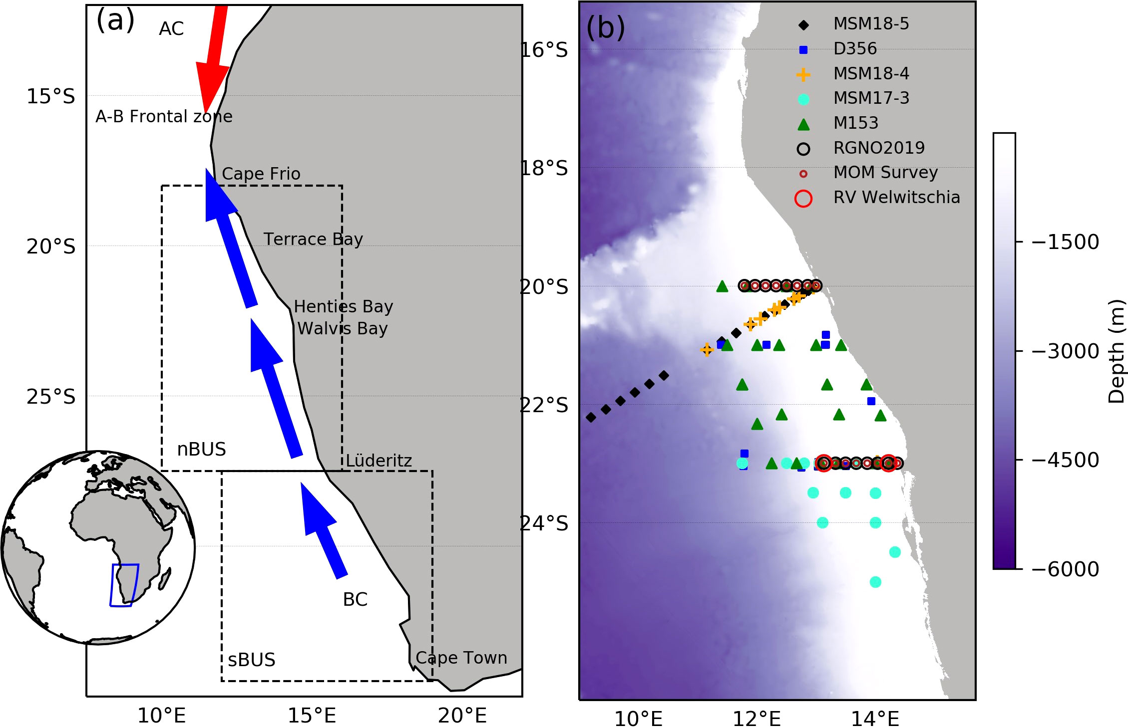
Figure 1 Map of western Africa showing the location of the Benguela Upwelling System (blue rectangle, inset). The BUS is partitioned into the northern (nBUS) and southern (sBUS) region separated by the Lüderitz upwelling cell at 27° S (A). The nBUS is bound by the cold water from the Benguela current (BC) and the warm water from the Angola current (AC) that converge at the Angola-Benguela frontal zone (A-B frontal zone). The right panel (B) shows bathymetry and the geolocations of stations sampled in the nBUS for Chl-a and phytoplankton community structure on the RV Meteor (M153) (green triangles) and Mirabilis RGNO2019 (black open circles). The geolocations of all additional cruise data (Table 1) are similarly identified with unique symbols as per the figure legend.

Marine phytoplankton contribute nearly half of the global primary production and serve as a direct food and energy source fuelling marine food webs at higher trophic levels (Field et al., 1998; Kwak and Park, 2020). In addition, phytoplankton blooms play an important role in global climate regulation through their contribution to the net annual uptake of atmospheric CO₂ (Arrigo et al., 1999; Caldeira and Duffy, 2000; Tortell et al., 2008; Pollard et al., 2009) and the production and release of aerosol particle precursors (e.g. dimethyl sulfide (DMS) gas and volatile organic carbons (VOCs)) that modulate cloud formation (Charlson et al., 1987; Stefels, 2000; Lizotte et al., 2017). This is of particular relevance in the nBUS, which is characterised by the presence of one of the largest and most persistent stratiform marine cloud decks that contribute to the variability and long-term trends of global albedo with impacts on both regional and global climate.

Marine phytoplankton encompass a diverse community of organisms, whose dominance varies in response to physicochemical variability in environmental conditions, that subsequently determines their ecological and biogeochemical function. For instance, diatoms are typically large cells that grow fast reaching high concentrations and due to their silica ballast and increased density, tend to sink fast and are considered very effective exporters of organic carbon to the deep ocean and important role players in the biological carbon pump (Smetacek, 1999; Brownlee and Taylor, 2002). Coccolithophores on the other hand are calcifiers that reduce seawater alkalinity and the carbonate concentration of surface waters in the process that forms their coccoliths (external calcium carbonate platelets), which impacts the ocean-atmosphere exchange of CO₂ (Brownlee and Taylor, 2002; Riebesell and Rost, 2004; Mcclelland et al., 2016). Together with dinoflagellates (Keller, 1989), coccolithophores have the highest intracellular dimethylsulfoniopropionate (DMSP) content and are considered prominent climate-active DMS gas producers (Archer et al., 2001; Lizotte et al., 2017) that may impact cloud formation and the radiation budget. Cyanobacteria on the other hand fix atmospheric nitrogen (N₂) in a process that contributes to N₂ input into the ocean to compensate for N₂ loss from denitrification (Agawin et al., 2007). Moreover, there are some bloom-forming and toxin-producing phytoplankton species (e.g. diatoms of Pseudo-nitzschia spp.), commonly referred to as harmful algal blooms (HABs) that are detrimental to both humans and aquatic life and have devastating consequences for the fisheries industry with important economic ramifications (Hoagland et al., 2002; Dermastia et al., 2022). As such, phytoplankton community structure and diversity is considered a key component of marine ecosystems as they have a direct impact on food web energy supply, fisheries and food security, ecosystem health and climate (Otero et al., 2020; Bestion et al., 2021). It is therefore crucial to study and understand phytoplankton community composition and its variability, especially in the face of global warming and the changing climate. The knowledge of the phytoplankton community composition and its sensitivity to climate forcing can provide a valuable understanding of ecological balance in marine ecosystems (Kruk et al., 2011), which can aid in informed policy drafting decisions for improved implementation of sustainable fisheries and environmental management for the protection and conservation of ecosystems.

Phytoplankton communities are highly dynamic and susceptible to seasonal (and intra-seasonal), interannual and long term variability in environmental drivers such as wind driven mixing (Louw et al., 2016), upwelling (Hansen et al., 2014) and radiative forcing. The nBUS is reported to have been progressively impacted by longer-term variability associated with climate change and other human-induced activities that have resulted in drastic changes to the ecosystem over the last decades. For example, fish catches and populations (sardines and anchovy most notably) have dramatically declined over the past five decades as a result of overfishing and possible environmental events such as hypoxia and Benguela Niños, that negatively affect organisms at both lower and higher trophic levels (Cury and Shannon, 2004). Moreover, upwelling indices indicate a decline in the frequency of upwelling events in recent years (2009 and 2014) in the nBUS (Lamont et al., 2018; Polonsky and Serebrennikov, 2020), with major implications for ocean productivity in support of marine food webs and the biological carbon pump. Consequently, there is a necessity for routine monitoring of phytoplankton as key roleplayers in this unique marine ecosystem for effective management as a scientific priority towards a better understanding and predictive ability of their role in maintaining ecosystem balance and climate feedback. Efforts to acquire long-term datasets towards adequately monitoring the nBUS for assessment of ecosystem changes have been made by the National Marine Information and Research Centre (NatMIRC, Namibia). The monitoring programme involves discrete in situ field observations collected quasi-monthly along two longitudinal transects off the coast of Namibia. These data have been used to assess trends in phytoplankton biomass (Louw et al., 2016), bloom-forming and toxin-producing diatoms of the genus Pseudo-nitzschia (Louw et al., 2017) and other environmental variables for nearly two decades. Field observations, although very useful in studying and monitoring marine ecosystems, are nonetheless severely limited in their regional and temporal coverage. Furthermore, they are labour intensive, costly and unable to provide near real-time monitoring observations.

Satellite ocean colour remote sensing observations have the ability to surpass traditional ocean sampling methods, that involve discrete samples collected on-board research vessels, owed to their large spatial and temporal scale resolution and ability to provide near real time information. Early studies of ocean colour remote sensing by satellite focused on the computation of global phytoplankton biomass using chlorophyll-a concentration ([Chl-a]) as a proxy, which improved our understanding of synoptic scale ocean primary production and biogeochemistry (O’Reilly et al., 1998). However, recognition of the importance of different phytoplankton taxonomic groups and their varying biogeochemical functions has compelled the need for the development of satellite products with the ability to resolve complex phytoplankton dynamics from space. At the forefront of this endeavour is the ability to provide information on the composition of the phytoplankton community (phytoplankton functional types – PFTs) in which each PFT represents a group of species aggregated according to distinct functional characteristics (e.g. size structure or taxonomic composition). More recent advancements in ocean colour remote sensing have seen the development of indirect techniques to derive phytoplankton functional types and size distribution such as the abundance-based algorithms that are based on [Chl-a] (Vidussi et al., 2001; Uitz et al., 2006; Hirata et al., 2011; Brewin et al., 2015). Spectral-based approaches on the other hand are more direct and rely primarily on the unique characteristics of light absorption and backscattering of different phytoplankton taxa, which can be retrieved from water-leaving reflectance. Variations in photosynthetic pigment composition, morphology, size, shape, and inner structure of different phytoplankton species is what drives the characteristics of inherent optical properties of surface waters that can subsequently be used to differentiate phytoplankton groups or species from satellite ocean colour remote sensing (Aguirre-Gomez et al., 2001; Vaillancourt et al., 2004; Soja-Wozniak et al., 2018). One example of this type of approach is the dual ratio approach, which utilises the ratio between 2 spectral bands to identify specific phytoplankton functional types. For instance, Bernard et al. (2005) used the 665 nm and 709 nm red/red band-ratio of the Medium Resolution Imaging Spectrometer (MERIS) sensor to identify HABs in the southern Benguela upwelling system (sBUS). Another approach uses spectral band differences to derive phytoplankton optical fingerprints. Typically, these algorithms are used to identify algal blooms of a particular taxa using three adjacent spectral bands in the red and near infrared or blue-green spectral regions that quantify the amplitude of a specific peak of absorption. One particularly useful example of this approach utilises the [Chl-a] fluorescence peak signal between 678 and 683 nm. Quantification of this signal, known as the fluorescence line height (FLH) (Letelier and Abbott, 1996; Kritten et al., 2020), is based on the height of the reflectance peak above a baseline formed between the two adjacent wavebands (Letelier and Abbott, 1996; Kritten et al., 2020). This approach has previously been applied to identify HABs in the coastal waters of SW Florida (Hu et al., 2005) and the sBUS (Smith and Bernard, 2020). Past and current ocean colour satellite sensors with appropriate wavebands in the red and near infrared (NIR) spectral regions, that are able to use these approaches, include the Moderate Resolution Imaging Spectroradiometer of aqua (MODIS-Aqua) [2002-present], the Ocean and Land Colour Imager (OLCI) [2016-present], and the MERIS sensors [2002-2012] (Letelier and Abbott, 1996).

Although there exist a limited number of satellite ocean colour remote sensing algorithms for aiding in the detection of multiple phytoplankton functional types (Aiken et al., 2007) and HABs in the sBUS (Bernard et al., 2005; Smith and Bernard, 2020), there is, to our knowledge, no satellite ocean colour remote sensing algorithm for detection of phytoplankton functional groups in the nBUS counterpart. While the regional abundance-based phytoplankton size class model of Lamont et al. (2019) for the BUS provides useful information on the variability of phytoplankton size functional types (picophytoplankton, nanophytoplankton and microphytoplankton), it is not able to approximate functional phytoplankton group composition (needed for the assessment of their various key ecological functions). The optical based algorithms derived by Aiken et al. (2007) and Smith and Bernard (2020) on the other hand are geared at providing information on the functional composition of phytoplankton for the sBUS (specifically diatoms, Pseudo-nitzschia, dinoflagellates, flagellates & mixed communities) and it cannot be assumed that they are applicable to the nBUS (or to different satellite products).

This study addresses the need for an ocean colour remote sensing algorithm for the detection of phytoplankton groups in the nBUS. It does so by first selecting the most suitable satellite sensor for the nBUS based on matchups between in situ and satellite (MODIS-Aqua, MERIS/OLCI) derived [Chl-a]. It subsequently follows a similar methodological approach to the algorithm developed for the sBUS by Smith and Bernard (2020) by identifying the spectral reflectance characteristics unique to stations dominated by particular phytoplankton functional groups. A combination of these unique optical characteristics is then used to derive an algorithm that can be applied to ocean colour data from the nBUS to elicit broad scale high resolution information on the likely distribution of the dominant functional types. Such an algorithm will allow observations of the spatio-temporal distribution and variability of key phytoplankton groups on an unprecedented scale in the nBUS, which is a scientific priority for understanding the marine food web and detecting its response to a changing climate in this globally important upwelling region.

2 Materials and methods

2.1 In situ data

2.1.1 Expeditions

This study focused on the nBUS off the coast of Namibia (Figure 1A) within the latitudes and longitudes of 20–26° S and 9–15° E, which included the Cape Frio, Central and the Lüderitz upwelling cells. Two expeditions were carried out on-board the RV Meteor (M153) and Mirabilis (RGNO2019) for data collection (Figure 1B). Cruise M153 took place from 15 February to 15 March 2019 covering both the northern and southern Benguela upwelling systems whereas cruise RGNO2019 took place from 9 to 10 of May 2019 covering 2 longitudinal transects (23 and 20° S). The stations sampled during the two expeditions (41 in total) are presented in Figure 1B. Seawater samples were collected in surface waters (0-5 m) using Niskin bottles attached to a conductivity-temperature-depth (CTD) carousel setup on-board the RV Meteor and Mirabilis. These data were supplemented with additional data from previous cruises in the region covering the period between 2001 and 2020 (Figure 1B; Table 1).

TABLE 1

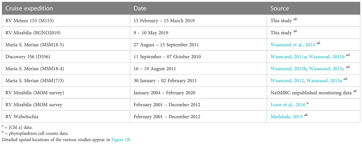
Table 1 Research expeditions in the northern Benguela upwelling system off Namibia where concurrent [Chl-a] and phytoplankton cell count samples were collected between 2001 and 2019.

2.1.2 Chlorophyll-a

For the M153 and RGNO2019 cruises total [Chl-a], 200 ml of seawater was filtered through glass microfiber filters (Whatman GF/F, 25 mm diameter, 0.7 μm pore size) and stored immediately in the freezer (-20 ˚C) for later analysis. Total [Chl-a] was determined following the method of Welschmeyer (1994). Chl-a was extracted from the GF/F filters by addition of 9 mL of 90% acetone for 24 hr in the dark at -20 ˚C. These were then transferred into glass tubes and fluorescence was measured using a Turner (Model 10AU) fluorometer. The [Chl-a] was determined from a seven-point [Chl-a] calibration curve and represented as equivalents of chlorophyll-a (μg l^-1).

2.1.3 Phytoplankton cell counts

For the M153 and RGNO2019 cruises phytoplankton cell enumeration and taxonomic identification, water from the Niskin bottles was transferred to 200 mL glass amber bottles and immediately preserved with acidic Lugol iodine solution, shaken gently and stored in the dark at room temperature for later analysis in the land-based laboratory. The Lugol-preserved phytoplankton cells were settled in a 25 ml glass/plastic chamber for 24 hours prior to analysis. The phytoplankton cells were identified and counted using a Zeiss Axiovert 200 inverted light microscope following the Utermöhl (1958) method. Cells were counted and identified to genus and to species level where possible. Approximately 400 cells were counted to achieve an estimation of cell concentration with ±10% precision, whereas at least 50-200 cells were counted when cells occurred in smaller concentrations with a precision of approximately 15–30% (Anderson and Throndsen, 2004). Although microscopic taxonomic identification of phytoplankton provides a resolution to genus and species levels, counted cells in this study were only grouped into diatoms, flagellates, dinoflagellates, cyanobacteria, coccolithophores, and others/unknown.

2.1.4 Additional in situ data sources

The M153 and RGNO2019 cruise datasets (detailed above) were supplemented with additional [Chl-a] and phytoplankton cell count data from multiple expeditions from publicly available, published and unpublished sources that were conducted in the nBUS covering the period between 2001 and 2020 (Table 1), to make a total pool of 252 stations. Data from the additional sources were similarly obtained from samples collected in the top 5 m and were similarly assessed for [Chl-a] using a fluorometer according to the principle of Welschmeyer (1994) and phytoplankton cell counts according to the method of Utermöhl (1958). The geolocations of the additional stations sampled are shown in Figure 1B with the respective sampling dates and data sources summarised in Table 1.

2.2 Satellite data

2.2.1 Data acquisition and processing

Daily Level-2 (L2) 1 km resolution ocean colour satellite data from the Moderate Resolution Imaging Spectroradiometer on board the Aqua satellite (MODIS-Aqua), the Medium Resolution Imaging Spectrometer (MERIS) on board Envisat, and the Ocean and Land Colour Instrument (OLCI) on board Sentinel-3 were obtained from the National Aeronautics and Space Administration (NASA) OceanColor Web (https://oceancolor.gsfc.nasa.gov/), MERIS catalogue and inventory (MERCI, http://meris-ds.eo.esa.int/oads/access/) and the Copernicus online data access website (CODA, https://coda.eumetsat.int/), respectively. The OLCI [Chl-a] data were derived from OLCI reflectance bands using the blended switching algorithm of Smith et al. (2018), which was developed specifically for the high biomass waters of the southern Benguela. The standard MODIS-Aqua [Chl-a] product is based on an empirical relationship derived from remote sensing reflectance (Rrs) between 440 and 670 nm and in situ [Chl-a]. This product is a combination of the standard OC3 algorithm (O’Reilly et al., 2000) and the colour index (CI) algorithm (Hu et al., 2012), where the OC3 algorithm is applied at [Chl-a] >0.2 mg m⁻³, whereas the CI algorithm is applied at [Chl-a]<0.15 mg m⁻³, and a weighted blending approach is applied between 0.15 and 0.2 mg m⁻³.

Other products obtained from MODIS L2 include the L2 flags, the nFLH and the remote sensing reflectance (Rrs) at 412, 443, 469, 488, 531, 547, 555, 645, 667 and 678 nm wavebands of the visible spectrum. The normalised fluorescence line height (nFLH, W m⁻² μm⁻¹ sr⁻¹) (Letelier and Abbott, 1996) is a standard product provided with the MODIS L2 Ocean colour data derived as follows:

$\begin{array}{ll}\mathit{n}\mathit{F}\mathit{L}\mathit{H} \mathit{=}{\mathit{L}}_{\mathit{w}}\mathbf{678} \mathit{-}{\mathit{L}}_{\mathit{w}}\mathbf{667} \mathit{-}[({\mathit{L}}_{\mathit{w}}\mathbf{748}\mathit{ }\mathit{-}{\mathit{L}}_{\mathit{w}}\mathbf{667})\mathit{*}(\frac{678-667}{748-667})] & (1)\end{array}$

where L_w is the normalised water-leaving radiance.

2.2.2 Matchups with in situ data

The L2 data from MODIS-Aqua, MERIS and OLCI were matched to field observation stations and extracted using a 5 x 5 pixel box centred around the in situ measurements as satellite navigation may not be accurate to a single pixel. The multi-pixel box increases the number of pixels of satellite retrievals and the possibility of a valid in situ matchup. A time window of ≤12 hrs between the satellite overpass and in situ observations was given preference as a temporal threshold for coincidence. However, when coincident satellite and in situ observations weren’t available within a 12 hr window, this criteria was relaxed to allow matchups to be considered within a ≤24 hr time window. The mean was then calculated for valid pixels within the 5 x 5 pixel box for [Chl-a], nFLH and Rrs at spectral bands in the visible range as outlined above, together with their respective statistical error metrics (e.g. standard deviations).

2.3 Data quality control

A set of quality control measures were adopted to minimise the inclusion and effect of bad/erroneous data from the L2 satellite data using a set of corrective measures as outlined in Figure S1. The L2flags product contains science and quality “flags”, with set atmospheric correction thresholds that were used to eliminate invalid pixels. Briefly, pixels were masked and excluded when flagged as “land” (pixel is over land), “clouds” (cloud contamination), “chlfail” (satellite ocean colour [Chl-a] algorithm failure), “higlint” (sunglint detected via reflectance exceeds threshold), “hisatzen” (sensor view zenith angle exceeds 60 °), “lowlw” (very low water-leaving radiance), and “hilt” (observed radiance very high or saturated). In an effort to remove invalid averaged matchup retrievals, further exclusion criteria were applied following Bailey and Werdell (2006), which removes matchups where fewer than 13 pixels were valid (i.e. where<50% of the 25 pixels within a 5 x 5 pixel box were valid). Furthermore, mean values whose standard deviations were >50% of the mean (indicative of large variability within the 5 x 5 pixel box) were removed to ensure spatial stability or homogeneity. Quality control measures applied to in situ [Chl-a] measurements included removal of measurements that were below the minimum detection threshold of the Turner fluorometer (<0.02 ug l^-1). Finally, in situ stations were excluded that were too close to one another and overlapped with a 5 x 5 pixel box (a flow diagram detailing the data quality control steps can be found in Figure S1 in the Supplementary Material).

2.4 Evaluation of MODIS-Aqua and MERIS/OLCI [Chl-a] algorithms

Statistical uncertainties between matchups of satellite ocean colour derived [Chl-a] and in situ fluorometric derived [Chl-a] were used to determine the most appropriate satellite sensor for algorithm development. The MERIS mission covered the period between 2002 and 2012, whereas OLCI and MODIS-Aqua were launched in 2016 and 2002, respectively, and both are still operational (at the time of writing). OLCI was developed on MERIS heritage with a similar spectral setup in order to provide continuity in algorithms and derived data; for this reason the match-ups from these two sensors were combined to create a single dataset. However, only the datasets covering the period between 2002-2012 and 2016-present were used for MODIS-Aqua so as to facilitate a fair comparison with MERIS/OLCI in this evaluation. Statistical metrics were used to quantify the agreement between in situ [Chl-a] and satellite-derived observations. Prior to the analysis, both the in situ and satellite retrievals were log-transformed. The statistics used for comparison were the mean relative error (MRE), mean absolute relative difference (MARD), median relative difference (MedRD), root mean squared error (RMSE) and relative bias, the exact equations of which can be found in the Supplementary Material indicated as equations S1 - S5.

In addition, a linear regression model was used to assess the degree of agreement between the in situ and satellite-derived [Chl-a]. The intercept, slope and coefficient of determination (R²) were computed.

2.5 Algorithm development

2.5.1 Subdividing the data by phytoplankton group dominance

The quality-controlled in situ data were subdivided according to phytoplankton group dominance. Dominance, in the context of this study, was typically achieved when a phytoplankton group contributed more than 50% to the total phytoplankton community abundance. It should be noted however that the nBUS is, for the most part, diatom-dominated (See Figure S3 on the Supplementary Material) and therefore the majority of the datasets were considered diatom dominated. For diatoms only, dominance was instead defined as a ≥70% contribution to the total phytoplankton community with a cell concentration of ≥500,000 cells l^-1. For flagellates and dinoflagellates, dominance was considered when cells were >50% of the total cell abundance. No cell count minima was set for these subsets as these stations typically did not reach high cell concentrations (i.e. >10⁶ cells L^-1).

Further analysis of the data showed dominance for dinoflagellates in both low [Chl-a] and high [Chl-a] (>4 μg l^-1) waters. Dinoflagellate dominance was thus subdivided into either low biomass or high biomass dominance (LB and HB, respectively). For HB dinoflagellate-dominated waters, dominance was considered when contributing >50% to the total cell abundance with cell counts of ≥10⁶ cells L^-1. Unfortunately, there were no in situ stations where either coccolithophores or cyanobacteria met the criteria for dominance. As such, this study focused only on identifying unique spectral characteristics of diatoms, flagellates and dinoflagellates from the satellite spectral matchup data. In addition, unique spectral characteristics were determined for a phytoplankton community that was considered mixed, i.e. when all the identifiable groups (including coccolithophores and cyanobacteria) and unidentifiable groups (i.e. classified as “other” in the phytoplankton taxonomic datasets) each contributed<50% to the total phytoplankton abundance with no set cell count minima.

2.5.2 Determining unique optical characteristics

The remote sensing spectral characteristics associated with dominance of the aforementioned phytoplankton groups were assessed using 4 approaches, namely 1) Rrs at different spectral bands, 2) dual-band Rrs ratios, 3) spectral band difference approaches and 4) a [Chl-a] abundance-based approach. For these approaches, the magnitude and shape of Rrs at 10 spectral bands were compared between waters dominated by the different phytoplankton groups. For dual-band spectral ratios, a total of 87 different ratio combinations among the violet, blue, green and red spectral regions were investigated. The spectral band difference or line height (LH) was calculated at eight different adjacent spectral band-triplets between 410 and 678 nm. LH is a measure of the height of the Rrs at a “signal” band above a baseline formed by any two given spectral bands, and was calculated as follows:

$\begin{array}{ll}\mathit{L}\mathit{H} \mathit{=} \mathit{R}\mathit{r}\mathit{s}\mathit{\_}\mathit{s}\mathit{i}\mathit{g}\mathit{n}\mathit{a}\mathit{l} \mathit{-}\mathit{R}\mathit{r}\mathit{s}\mathit{\_}\mathit{l}\mathit{e}\mathit{f}\mathit{t} \mathit{-}(Rrs\_right -Rrs\_left)\times (\frac{{\lambda }_{signal}- {\lambda }_{left}}{{\lambda }_{right}- {\lambda }_{left}})& (2)\end{array}$

Where λ is the wavelength value at a spectral band of interest, Rrs_signal is the Rrs value at the signal band centred between two spectral bands, Rrs_left is the Rrs to the left of Rrs_ signal, Rrs_right is the Rrs to the right of Rrs_ signal, λ_signal is the λ value of Rrs_signal whereas λ_right and λ_left are the λ values of Rrs to the right and left of the Rrs_signal respectively. The nFLH, a downloadable L2 MODIS-aqua product as described in the “data acquisition” section above, is a well-known example.

Spectral reflectance peaks may occur near 685 nm in low to moderate [Chl-a] waters as a consequence of [Chl-a] fluorescence emission (Gordon, 1979). However, this [Chl-a] fluorescence peak may be masked in high phytoplankton biomass waters (e.g. [Chl-a] > 20 μg l^-1) as a result of increased absorption and backscattering by phytoplankton coupled with increased water absorption (Gordon, 1979; Schalles, 2006; Gilerson et al., 2007); this is often observed as a shift in the red reflectance peak towards the NIR region. In this study, we quantify this red shift as a ratio between a red (Rrs667) and NIR (Rrs748) spectral bands, the red-NIR ratio (RNR). The Rrs748 is not provided in the standard L2 MODIS files, and is instead calculated from the available nFLH, Rrs667 and Rrs678, and solar spectral irradiance values from Thuillier et al. (2003) as follows:

$\begin{array}{ll}\mathit{R}\mathit{r}\mathit{s}\mathbf{748} = ((\frac{\mathbf{81}*\mathit{R}\mathit{r}\mathit{s}\mathbf{678}*\mathbf{1481.93}}{\mathbf{11}})-(\frac{\mathbf{81}*\mathit{n}\mathit{F}\mathit{L}\mathit{H}}{\mathbf{11}})-(\frac{\mathbf{70}*\mathit{R}\mathit{r}\mathit{s}\mathbf{667}*\mathbf{1517.73}}{\mathbf{11}}))÷\mathbf{1288.25}& (3)\end{array}$

The RNR was then calculated as:

$\begin{array}{ll}\mathit{R}\mathit{N}\mathit{R} \mathit{=} \frac{\mathit{R}\mathit{r}\mathit{s}\mathbf{748}}{\mathit{R}\mathit{r}\mathit{s}\mathbf{667}}& (4)\end{array}$

[Chl-a] was used as a proxy for phytoplankton abundance for the development of the abundance-based algorithm, based primarily on the understanding that at high biomass the phytoplankton community was dominated by either diatoms or dinoflagellates.

2.6 Statistical analysis

Box and whisker plots were used to graphically display the distribution and statistical parameters of the data which included the median (Q₂), lower (Q₁ or 25^th percentile) and upper (Q₃ or 75^th percentile) quartiles as well as the lower (Q₀ or minimum) and upper (Q₄ or maximum) extremes of the datasets. The box represents the interquartile interval where 50% of the data is distributed. The whiskers display the lower (minimum) and upper (maximum) extremes of the datasets. Outliers were defined as data points that are 1.5 times higher than the interquartile range (IQR) calculated from both the lower (Q₁) and upper (Q₃) quartiles and indicated as circles in the box and whisker plots. The 25^th and 75^th percentiles were used to define optical signature thresholds associated with dominance of the phytoplankton groups under investigation. The Matplotlib, Scipy.stats, Numpy and Sklearn.metrics Python (version 3.7.3) packages were used for statistical data analysis.

3 Results

3.1 Evaluation of MODIS-Aqua and MERIS/OLCI [Chl-a] algorithms in the nBUS in comparison with in situ data

For both MODIS-Aqua and MERIS/OLCI sensors, the quality-controlled [Chl-a] match-up datasets were used for comparison (Figure 2), which covered the in situ [Chl-a] range of 0.18 – 36.25 μg l^-1. The matchup datasets were reduced from n=56 and 54 stations to n= 36 and 37 for MODIS-Aqua and MERIS/OLCI respectively, following the application of the stringent quality control measures outlined in Figure S1. Scatter plots of the comparisons between in situ and satellite [Chl-a] are shown in Figures 2A, B with the data that passed quality control being easily identified from the raw data that did not. Statistical parameters of the linear regressions between the quality-controlled data showed a positive correlation between in situ [Chl-a] and satellite retrievals. The Pearson correlation coefficient (r) was similar for both sensors, with MODIS-Aqua having a slightly lower correlation (r = 0.67) than that of MERIS/OLCI (r = 0.68) (Figure 2C).

FIGURE 2

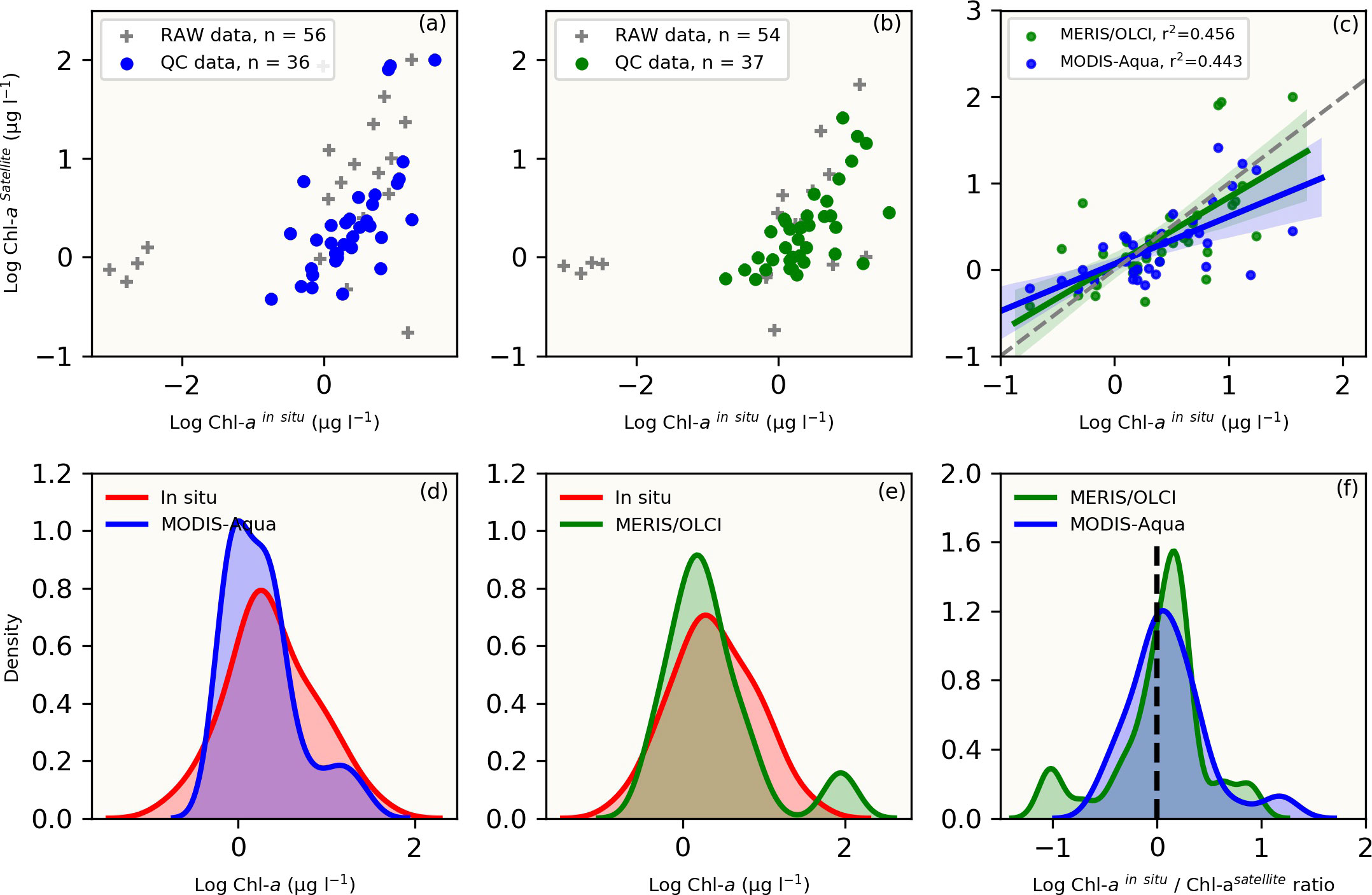
Figure 2 The top panel shows raw and quality-controlled (QC) in situ versus satellite [Chl-a] data for the (A) MODIS-Aqua (blue dots), (B) MERIS/OLCI (green dots) and raw data (grey crosses) (C) linear regression statistics with 95% confidence intervals (shaded areas) for the QC [Chl-a] comparisons between MODIS-Aqua (blue shaded line) and MERIS/OLCI (green shaded line). The number of QC datasets used for comparative analysis (n) are indicated. The bottom panel compares the data distribution between in situ (red) and satellite-derived [Chl-a] using the Kernel density estimation (KDE) plots for (D) MODIS-Aqua (blue) and (E) MERIS/OLCI (green). (F) is a direct comparison of the ratio of in situ to satellite [Chl-a] between the two sensors (blue: MODIS-Aqua; green: MERIS/OLCI). All datasets were log-transformed prior to plotting and statistical analysis.

Both sensors showed a similar [Chl-a] distribution when compared to co-located in situ [Chl-a] observations (Figures 2D, E), with MERIS/OLCI having a few data points outside the maximum range of the in situ [Chl-a] centred at ~2 ug l^-1 (Figure 2E). In order to better understand the distribution between the datasets, the log-transformed [Chl-a]^{in situ/}[Chl-a]^satellite ratio was determined (Figure 2F) and showed that the apex of distribution for MODIS-Aqua was closer to zero (i.e. the 1:1 line), while the majority of the data was distributed within a positive ratio for both satellites. This positive distribution is indicative of a general tendency for both sensors to underestimate in situ [Chl-a]. This was similarly evident for both sensors in the negative mean relative error (MRE) (-44.6% and -38.7% for MERIS/OLCI and MODIS-Aqua respectively) and the negative median relative errors (-32.5% and -13.9% for MERIS/OLCI and MODIS-Aqua respectively) (Table 2). Similar findings (i.e. overestimation at lower [Chl-a] and underestimation at higher [Chl-a]) were reported by Dogliotti et al. (2009) for MODIS-Aqua when compared with SeaWiFS for the Argentinean Patagonian continental shelf between 38° S and 55° S, which they attributed to differences in phytoplankton composition across a similar range of [Chl-a].

TABLE 2

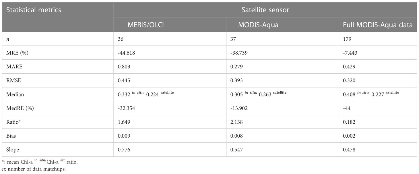
Table 2 Statistical metrics used for comparison of satellite-derived and in situ [Chl-a] match-ups between the MODIS-Aqua and MERSI/OLCI sensors in the northern Benguela.

Comparison of MODIS-Aqua to in situ [Chl-a] for the full dataset (n=179) (i.e. not limited to the time period that coincided with MERIS/OLCI), showed similar statistical results (data distribution and error margins) (Figures 3A, B). An overall [Chl-a] underestimation tendency is similarly observed as shown in Figures 3C, C inset), the statistical metrics of which (MRE, MARE, RMSE, MedRE and Bias) are also summarised in Table 2, with a tendency to overestimate at very low [Chl-a] concentrations (Figure 3D). Overall, it can be observed from the log ratio distribution in Figure 3D that the MODIS-Aqua satellite algorithm compared well with in situ measurements and that the error margins improved when the expanded full data matchups were used.

FIGURE 3

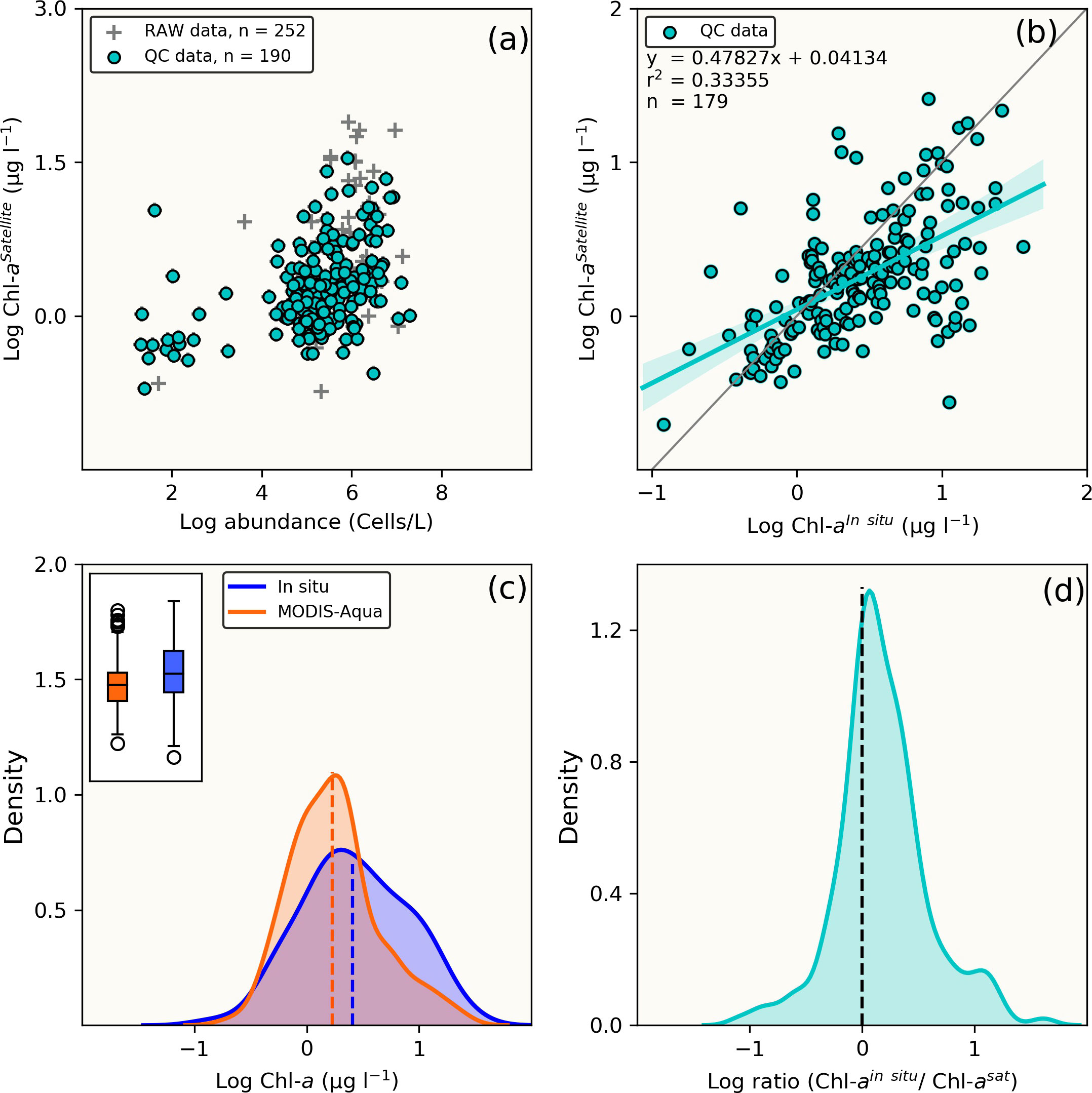
Figure 3 Comparison between full (n = 179) in situ [Chl-a] dataset and MODIS-Aqua satellite match-up retrievals. (A) Raw and quality controlled datasets, (B) Linear statistical regression of QC Chl-a between in situ and MODIS-Aqua match-ups, (C) Comparative overview of [Chl-a] distribution from in situ and MODIS-Aqua using the Kernel density estimate plots and boxplots (inset). The dotted vertical lines indicate the mean [Chl-a] and (D) distribution plot of log-transformed [Chl-a]^{in situ/}[Chl-a]^satellite ratio.

3.2 Deriving phytoplankton optical fingerprints from ocean colour remote sensing

3.2.1 Remote sensing reflectance

Figure 4 shows the Rrs characteristics across 10 spectral wave bands in the visible range for oceanic waters dominated by different phytoplankton community groups, namely diatoms, HB and LB dinoflagellates, flagellates and mixed assemblage. These Rrs spectra showed considerable differences in magnitude and shape among the phytoplankton groups, which is subsequently exploited for deriving optical fingerprints that are characteristic for specific groups. For example, the Rrs minima observed in the longer wavelengths (i.e. red region: 645, 667 and 678 nm) is evident for all phytoplankton groups except HB dinoflagellates, whose Rrs minima is in the shorter violet/blue region (412/443 nm) (Figure 4). LB dinoflagellates had a characteristic maxima in the violet/blue region (412/443 nm) of the spectra, while for both HB dinoflagellates and flagellates, the Rrs magnitude increased with increasing wavelength from violet/blue-to-green with the Rrs maxima located in the green spectral region (555 nm) for HB dinoflagellates & (547 nm) for flagellates.

FIGURE 4

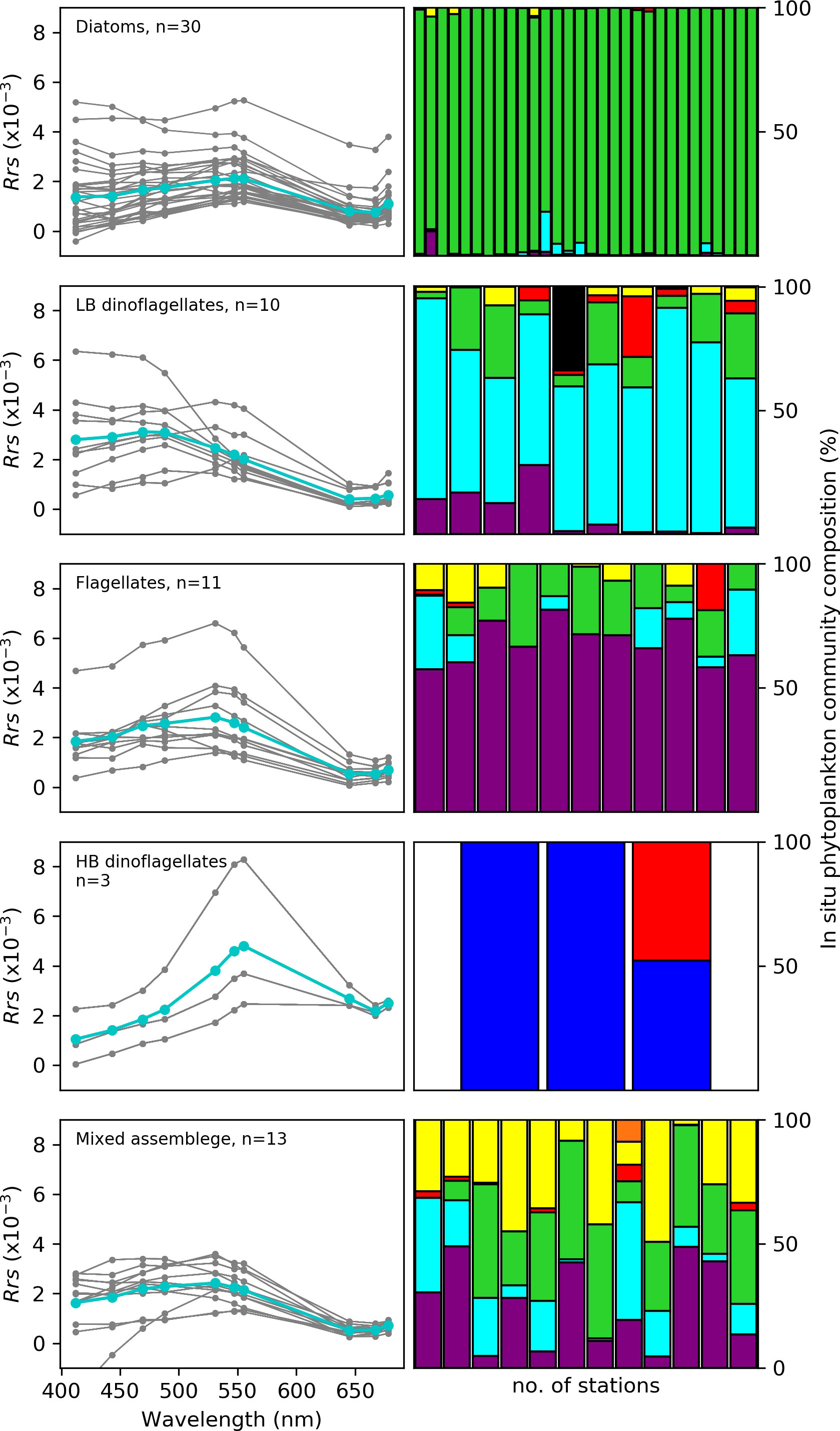
Figure 4 The remote sensing spectral reflectance (Rrs) in the visible range of the spectrum with wavebands at 412, 443, 469, 488, 531, 547, 555, 645, 667 and 678 for samples from the nBUS waters dominated by the phytoplankton groups (Diatoms, flagellates, low (LB) and high (HB) biomass dinoflagellates and Mixed assemblage from the MODIS-Aqua satellite sensor are shown in the left panel. The cyan line indicates the mean Rrs at each spectral band and the number of match-ups (n) are indicated. The coloured bars on the right panel represent the corresponding % phytoplankton community composition at each station per phytoplankton group. The colours refer to diatoms (green), LB dinoflagellates (turquoise), HB dinoflagellates (blue), flagellates (purple), coccolithophores (red), cryptophytes (orange), cyanobacteria (black) and other/unknown (yellow).

3.2.2 Remote sensing reflectance spectral band-ratios

Multiple spectral band-ratios were investigated to identify optical signatures typical of waters dominated by the various phytoplankton groups under investigation. Boxplots of band-ratios were used to assign thresholds associated with the probability of dominance by each group based on the 25^th and 75^th percentiles of the datasets (Figures 5A–D). The green/violet, blue/violet, violet/violet, blue/blue and red/violet spectral band-ratios yielded no obvious unique spectral thresholds that may be assigned to dominance of any group as the data distribution (box plots) were within similar overlapping ranges (data not shown). However, characteristic dual spectral band-ratio thresholds were identified for red/blue (Rrs678/Rrs488), green/green (Rrs547/Rrs531), red/red (Rrs645/Rrs678) and green/blue (Rrs555/Rrs488) ratios that could describe a high probability for the presence of diatoms, LB dinoflagellates, HB dinoflagellates, flagellates and mixed communities. These differentiations are graphically represented in Figures 5A–D and the threshold values summarised in Table 3. The LB dinoflagellates had characteristically low red/blue, green/green and green/blue ratios, while diatoms occupied an intermediate green/green and green/blue band-ratios. The HB dinoflagellates had characteristically high green/green, red/red and green/blue band-ratios (Figures 5A–D blue shading). Although HB dinoflagellates typically had a higher red/blue ratio than diatoms, they expressed a large overlap (Figure 5A teal shading). Flagellates overlapped the mixed assemblage in the green/green ratio (Figure 5B magenta shading) but occupied a relatively unique, yet narrow distribution band in the red/blue ratio (Figure 5A purple shading), while the mixed community had a distinct red/red band-ratio (Figure 5C orange shading).

FIGURE 5

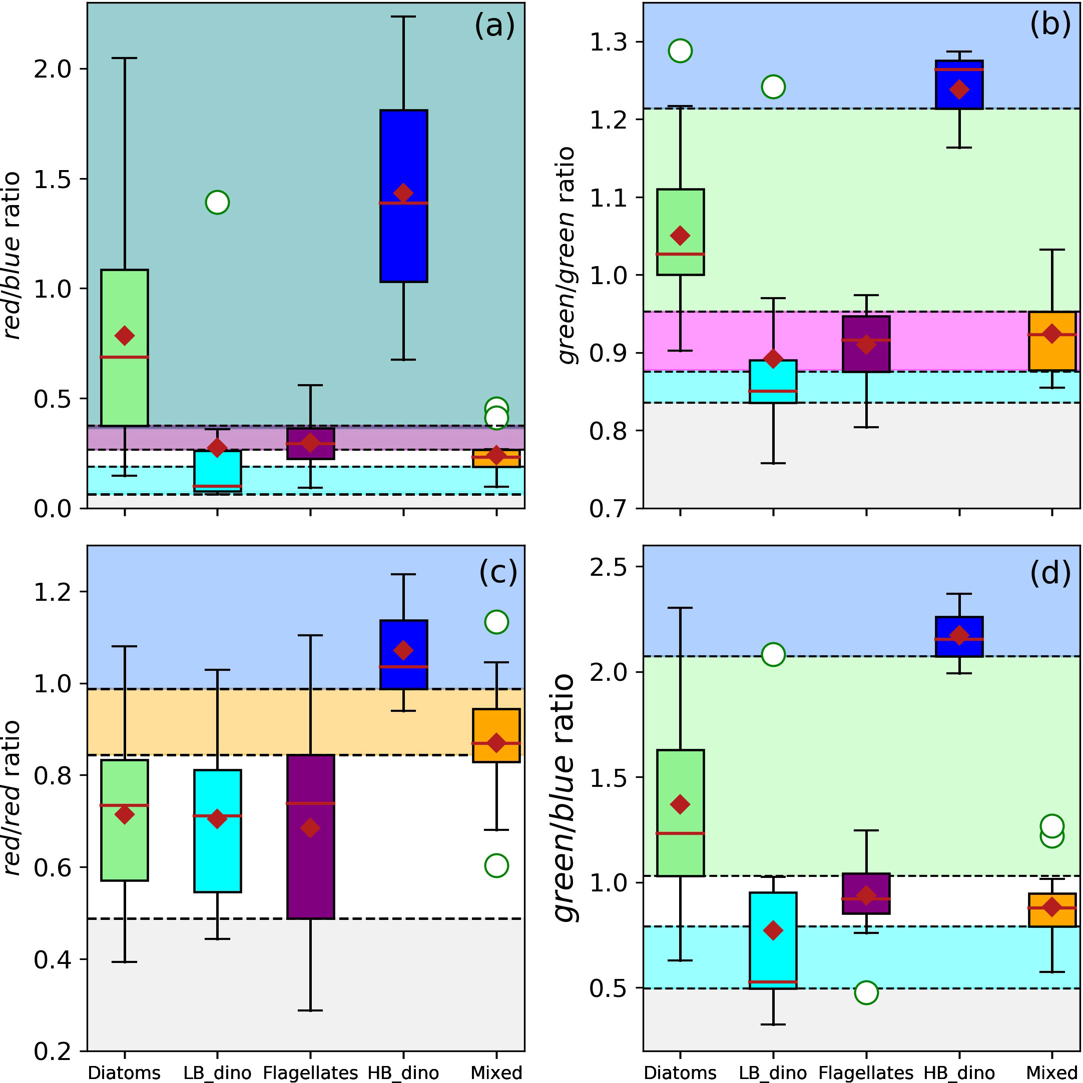
Figure 5 Boxplots of the dual-spectral band ratios for waters associated with dominance of diatoms, LB dinoflagellates (LB_dino), flagellates, mixed community and HB dinoflagellates (HB_dino). The thresholds of the red/blue (Rrs678/Rrs488) (A), green/green (Rrs547/Rrs531) (B), red/red (Rrs645/Rrs678) (C, D) green/blue (Rrs555/Rrs488) band-ratios are indicated by the dashed horizontal lines and colour shaded bands (light green = Diatoms; cyan = LB dinoflagellates, purple = Flagellates, blue = HB dinoflagellates, orange = Mixed, teal = Diatoms/HB dinoflagellates, magenta = Flagellates/Mixed). Statistical parameters such as the median, mean and outliers are indicated as the red line, red diamond and white circles respectively.

TABLE 3

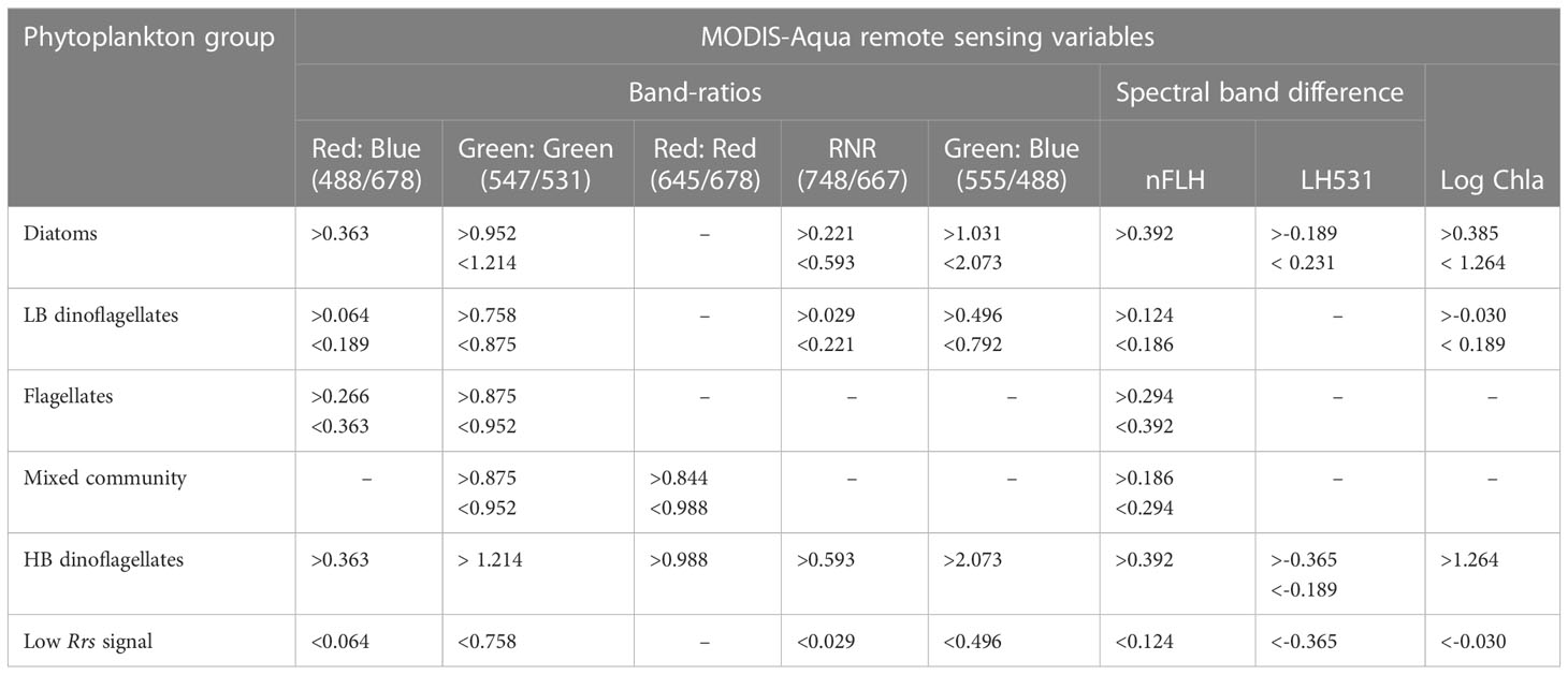
Table 3 Summary of MODIS-Aqua spectral threshold characteristics for waters dominated by various phytoplankton groups in the nBUS.

3.2.3 Spectral band difference, RNR and [Chl-a]

The characteristic spectral band difference, RNR and [Chl-a] for detection of conditions associated with dominance of diatoms, LB dinoflagellates, HB dinoflagellates, flagellates and mixed communities were investigated and are graphically represented in Figure 6, with thresholds indicated. The threshold values for spectral band difference are summarised in Table 3. Both diatom and HB dinoflagellate-dominated waters shared a characteristic of high nFLH (Figure 6A, teal shade), although diatoms displayed the highest nFLH by comparison. However, HB dinoflagellates had a higher RNR and [Chl-a] biomass and a lower line height at 531 nm (LH531) than diatoms (Figures 6B–D). Although generally having similar spectral features to other phytoplankton groups, the flagellate-dominated waters represent a discernible nFLH range between diatoms and dinoflagellates (Figure 6A, purple shade). Unlike their high biomass counterparts, the LB dinoflagellates had the lowest nFLH, RNR and were generally dominant in low [Chl-a] conditions (Figures 6A–C). The spectral band difference and [Chl-a] features of the mixed community showed no unique characteristics and were thus indistinguishable from other groups using these approaches. It should be noted that several line heights were calculated at various spectral wavelengths and were distributed similarly for all the groups (data not shown). Generally, variability in line height was observed in the green spectral regions (531, 547 and 555 nm) with a resolution between diatoms and HB dinoflagellates while the remaining groups showed no obvious line height thresholds unique to them. Important to note is that a final category was defined as “low Rrs signal”, where the Rrs signal was considered too low to confidently retrieve any discernible signal due to a low signal-to-noise ratio, these low Rrs criteria were defined by the lowest 25th percentile of the distribution of each Rrs variable and are summarised in Table 3.

FIGURE 6

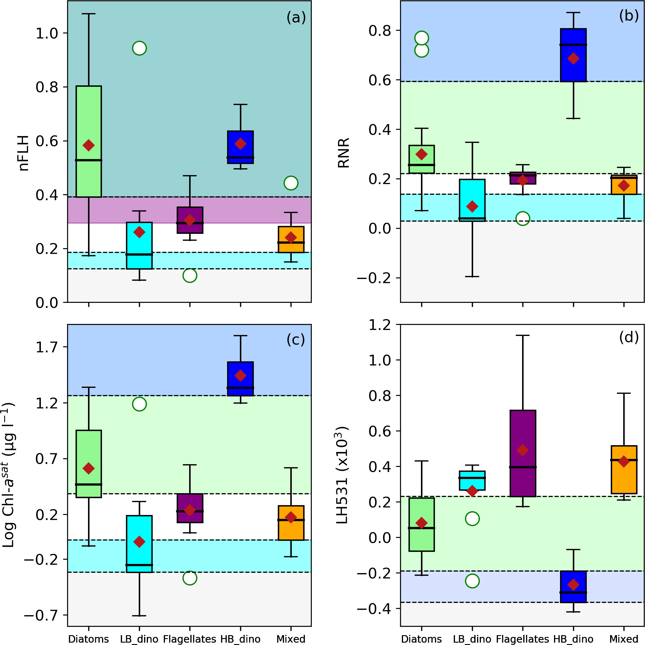
Figure 6 Boxplots of (A) nFLH, (B) RNR, (C) log-transformed [Chl-a] and (D) line height at 531 nm (LH531) for waters associated with dominance of Diatoms, LB dinoflagellates (LB_dino), Flagellates, HB dinoflagellates (HB_dino) and Mixed communities. The threshold ranges are indicated by the dotted horizontal lines and colour schemes (green = Diatoms; cyan = LB_dino; purple = Flagellates; blue = HB_dino; red = Mixed; teal scale = Diatoms/HB dinoflagellates). The median, mean and outliers are indicated as the bold black line, red diamond and white circles respectively.

3.3 Algorithm development

Our approach to detecting phytoplankton community characteristics from space investigates statistical thresholds based on [Chl-a] biomass, dual band-ratios and spectral band differences to exploit small variations in the Rrs characteristics associated with dominance of specific phytoplankton groups. If the Rrs spectrum from a pixel is within a range defined by the threshold values for waters associated with the dominance of a particular phytoplankton group, then it is assigned to reflect the likelihood of that phytoplankton group being dominant. These thresholds are summarised in Table 3.

Given the identified thresholds for the various phytoplankton groups from the remote sensing variables indicated in Table 3, the next step was to determine the most suitable variables for algorithm development. To do this, we assess 1) the algorithms’ ability to confidently classify/distinguish multiple phytoplankton groups, 2) the characteristics of the linear relationship between the variables in Table 3 and [Chl-a], with the understanding that biomass is likely to influence the spectral characteristics of Rrs and 3) the range in [Chl-a] that is typical for each of the defined thresholds for the various phytoplankton groups, favouring variables that allow for the classification of a number of phytoplankton groups within a similar range of [Chl-a]. While some algorithms are suitable for detection of specific phytoplankton groups during high biomass blooms, we embark on developing an algorithm that is suitable for the detection of dominant groups even in low [Chl-a] (non-bloom) conditions. To assist with the assessment of these criteria, we examined the linear relationship between the Rrs variables and [Chl-a] (Figures 7A–F). Each of the three criteria is presented in detail below:

FIGURE 7

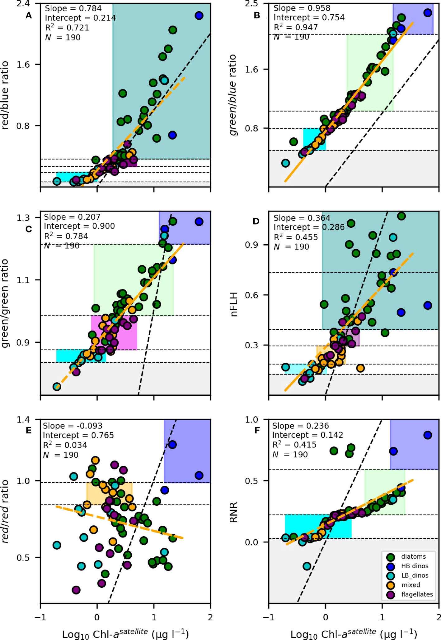
Figure 7 Linear regression analysis between [Chl-a] against the (A) red/blue, (B) green/blue, (C) green/green, (D) nFLH, (E) red/red and (F) RNR band-ratio,algorithms, [Chl-a] data was log-transformed prior to analysis. The linear regression is shown by the dashed orange line. The black dotted line represents the theoretical 1:1 relationship. The coefficient of determination (R²), slope, intercepts and number of samples (N) are indicated. The samples representing dominance by diatoms, LB dinoflagellates (LB_dino), HB dinoflagellates (HB_dino), flagellates and mixed communities are indicated as green, cyan, blue, purple and orange dots respectively. The shaded areas denote the unique spectral characteristic thresholds for each group (green = diatoms, cyan = LB dinoflagellates, orange = mixed, purple = flagellates, blue = HB dinoflagellates, magenta = mixed/flagellates, teal = diatoms/HB dinoflagellates).

1) Can the Rrs variable confidently distinguish multiple PFTs?

In Figure 7A, the red/blue ratio defining flagellates and LB dinos are tightly clustered together with a low range of variability in the optical identifier making it difficult to distinguish them from each other. In addition, there was overlap in the range of diatoms and HB dinos. In Figure 7E, although more broad, it is clear that the majority of PFTs share a similar range of variability in the red/red ratio hampering an ability to identify the majority of PFTs.

2) Is variability in the Rrs signal biomass dependent?

A strong positive linear relationship and slope close to 1 was observed between [Chl-a] and the red/blue (r²= 0.721, slope = 0,784) and green/blue band-ratios (r²= 0.947, slope = 0.958) (Figures 7A, B, respectively), suggesting that these optical signals were, for the most part, biomass-driven. This is not surprising as the global ocean colour remote sensing algorithms for [Chl-a] retrieval from the MODIS-Aqua are based on the ratio of the red, blue and green spectral bands. Using biomass as a criteria (or any other variable that is strongly dictated by biomass) constrains the algorithm’s ability to detect a particular phytoplankton group outside of the assigned biomass range. This is highlighted by the absence of any overlap (i.e. vertical stacking) of the PFT boxes defined by the green/blue ratio in Figure 7B.

3) Is there overlap in the range of [Chl-a] for different PFTs?

Although the green/green band-ratio (Figure 7C) showed a similar positive linear relationship with [Chl-a] (r²= 0.784), it had a much lower slope (slope = 0.207), while nFLH and RNR both displayed weak linear relationships and lower slopes (r²= 0.455, slope = 0.364, Figure 7D and r²= 0.415, slope = 0.236, Figure 7F, respectively). When the slope is more gradual (i.e. Figure 7C, D, F), the range in [Chl-a] encompassed for each Rrs identifier is broader. Moreover, for these optical signatures, there is a larger range of variability evident in the Rrs identifiers for a similar range in [Chl-a] concentration. This is highlighted by the overlap in [Chl-a] among the groups but with varying Rrs signatures (i.e. the vertical stacking of PFT boxes across a similar range of [Chl-a]).

Given the above, the red/blue (Figure 7A), green/blue (Figure 7B), and red/red (Figure 7E) band-ratios were not considered further and eliminated as viable variables for further algorithm formulation. On the other hand, nFLH and the green/green band-ratio were considered the most suitable candidates for further development of the phytoplankton PFT algorithm. In addition, the RNR spectral band-ratio was also considered, in particular as a means of discriminating dinoflagellates from diatoms under high biomass conditions (i.e. when [Chl-a] > 8).

Unsurprisingly, there are overlaps in some optical signatures of different phytoplankton groups. For instance, both diatoms and HB dinoflagellates have an overlapping nFLH range (0.392) (Figure 7D, teal shading) and both flagellates and mixed communities share a similar range in the green/green ratio (Figure 7C, magenta shading). However, they have other unique signatures that allow a combination of criteria to be used to separate them out. For example, in the case of diatoms and HB dinoflagellates we use the green/green and RNR band-ratios to distinguish the two groups (Figure 8A). That is, if nFLH is > 0.392 then that pixel can be classified as either a diatom or a HB dinoflagellate. However, if the RNR is > 0.593 and the green/green ratio is >1.214 then that pixel is more likely to be dominated by HB dinoflagellates and as such is assigned that category. However, if the green/green ratio is<1.214 and the RNR is< 0.593 then it is more likely a diatom and is assigned as such within the given nFLH range. The use of combined algorithms of spectral characteristics increases the robustness and reliability of the algorithm, while at the same time allowing groups to be detected across a broad range of [Chl-a]. For example, diatoms can be detected across the full range of their green/green and nFLH criteria, so long as the RNR is not high, in which case it is assigned to HB dinos.

FIGURE 8

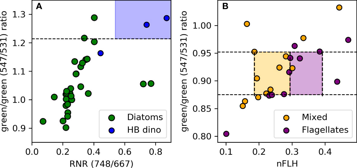
Figure 8 (A) Discrimination of diatom from dinoflagellate blooms based on differences in their RNR signals given their shared high green/green (>1.214) band-ratio and nFLH (>0.392) spectral characteristics. (B) Flagellates and the mixed communities are distinguished based on their nFLH spectral characteristics given their similarities in their green/green. and nFLH spectral characteristics. The blue, orange and purple colour shadings indicate the spectral characteristics unique to HB dinoflagellates, mixed community and flagellates respectively.

Similarly, in the case of flagellates and mixed communities, despite an overlap in their green/green ratio, they could be distinguished from each other based on the unique statistical signature within their nFLH distribution (Figure 6A). That is, a pixel with a green/green band-ratio between 0.875 and 0.952 could be classified as either flagellate-dominated or a mixed community. However, if the nFLH is between 0.294 and 0.392 then it would be assigned to reflect flagellate dominance, whereas if the nFLH is between 0.186 and 0.294 it would reflect a mixed community (Figure 8B). LB dinoflagellates on the other hand have a distinct green/green band-ratio and nFLH threshold, and unlike diatoms, HB dinoflagellates, flagellates and mixed community, were distinguished using individual thresholds of the green/green band-ratio and nFLH for their detection. Pixels are regarded as ‘other/unknown’ phytoplankton when no algorithm threshold criteria is met. A flowchart of the algorithm decision making tree (application) for discrimination and classification of the various phytoplankton groups in the nBUS is shown in Figure S2 of the Supplementary Material.

3.4 Algorithm validation

The algorithm was tested for accuracy and compared against randomly selected independent in situ datasets for diatoms. Unfortunately, this was only possible to do with diatoms, as this was the only phytoplankton group that dominated at enough stations to allow partitioning of the datasets into testing and validation groups. All other groups had so few stations in which they dominated that all had to be used to derive the most robust algorithm possible. The diatom validation was achieved by comparing observations with predictions (considered when in situ validation datasets’ Rrs spectra fell within the algorithm detection thresholds). It should be noted that diatom dominance of validation datasets were similarly defined using the same criteria used to define diatom dominance for training datasets. A total of 7 datasets were used for validation of the diatom detection component of the algorithm for the nBUS. The quantitative validation results for diatoms, calculated as overall accuracy of the algorithm, was calculated as follows:

$\begin{array}{ll}\mathit{A}\mathit{l}\mathit{g}\mathit{o}\mathit{r}\mathit{i}\mathit{t}\mathit{h}\mathit{m} \mathit{a}\mathit{c}\mathit{c}\mathit{u}\mathit{r}\mathit{a}\mathit{c}\mathit{y} \mathbf{=} (\frac{\mathit{C}\mathit{c}}{\mathit{T}\mathit{c}}) \mathbf{\times } \mathbf{100}\mathbf{\%}& (5)\end{array}$

where Cc is the correct classifications and Tc is the total classification from the independent diatom dominance datasets not used in the algorithm training datasets. We compared the optical characteristics of the validation data for stations dominated by diatoms against the algorithm thresholds and our algorithm compared well with the independent in situ observations of diatom dominance. Of the 7 stations, 5 matched with algorithm thresholds (i.e. were correctly classified by the algorithm). This translates to a percentage accuracy of 71.429%. The validation results demonstrate the algorithm’s ability to translate MODIS-Aqua Rrs observations to distributions of phytoplankton communities in the nBUS. The diatom-dominated stations that were not correctly classified had lower green/green and nFLH values that were below our algorithm’s minimum detection thresholds. In addition, they occurred in waters with low [Chl-a] that were between 1-2 μg l^-1. However, we were able to correctly classify 3 stations of diatoms within the same [Chl-a] range based on their Rrs characteristics.

Although we did not have sufficient in situ HB dinoflagellate dominated station data to validate the algorithm, we were able to demonstrate its ability to detect a known dinoflagellate bloom identified in the southern Namaqua Benguela upwelling system 3.5 km from Lambert’s Bay (Cape Town, South Africa) in the sBUS (Fawcett et al., 2007) (Figure 9).

FIGURE 9

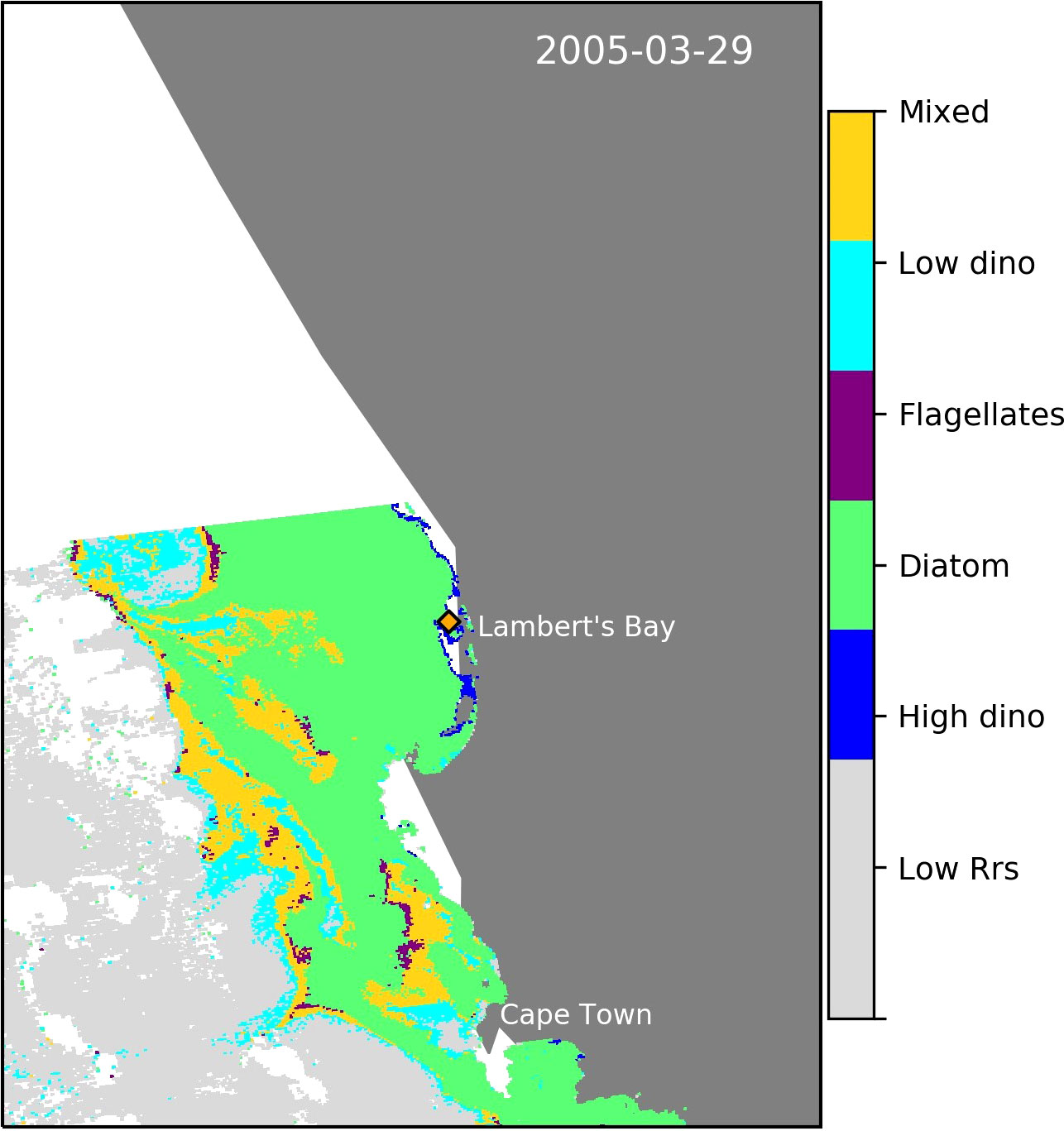
Figure 9 Evidence of the algorithm’s ability to detect a known harmful dinoflagellate bloom in the sBUS (Fawcett et al., 2007). The sampled coastal station in Lamert’s Bay is indicated by the orange diamond.

4 Discussion

Forming the base of marine food webs, phytoplankton are key ecological role players in upwelling systems and the global ocean. Knowledge of their composition and their regional, seasonal and interannual distribution and trends is key to understanding possible climate-linked ecosystem changes with implications on ecosystem health, economy, food security and climate response. Satellite remote sensing is one of the only tools that can provide the spatial, temporal and multi-decadal data information on phytoplankton needed to adequately investigate their important role in ecosystem function. Thus, there is a need for ocean colour remote sensing algorithms that can discriminate between phytoplankton functional types. Discrimination between diatoms and dinoflagellates is particularly relevant to ecology, local aquaculture and recreational activities as some of the bloom-forming and toxin-producing species belonging to these groups have been reported in the nBUS (Dijerenge, 2015; Louw et al., 2017; Gai et al., 2018), which may be harmful to both marine life and humans. Substantial work has been done using ocean colour algorithms and modelling techniques to detect phytoplankton community structure in the southern Benguela (Bernard et al., 2005; Aiken et al., 2007; Evers-King, 2014; Smith and Bernard, 2020), but none as yet for the northern Benguela. This study is the first to derive an ocean colour remote sensing algorithm for the nBUS using a large compiled in situ microscopy dataset with satellite match-ups for detection and mapping of the most frequently encountered phytoplankton groups.

4.1 Determining the most appropriate satellite sensor for algorithm development

The first step in this endeavour was to determine which satellite product to use based on the availability of spectral bands in the red and near infrared regions. We approached this decision by comparing the two available ocean colour remote sensing algorithms of [Chl-a] to in situ measurements in order to test how well they performed in the high biomass coastal waters of the nBUS. MODIS-Aqua provided more data near the 1:1 ratio than MERIS/OLCI, suggesting a good approximation of in situ [Chl-a] (Figure 2F). Although MERIS/OLCI had a higher slope (0.766) than MODIS-Aqua (0.547), it contained more statistical errors (MRD, MAE, RMSE, MARD) against in situ [Chl-a] than MODIS-Aqua (as summarised in Table 2). We are however cognisant that fluorometry-derived Chl-a may be biased towards higher concentrations when compared to high-performance liquid chromatography (HPLC), particularly in the presence of Chl-c due to potential overlap in emission spectra (Moutier et al., 2019). It should however be noted that the Chl-a datasets used in the current study were measured using the non-acidification technique (Welschmeyer, 1994), which minimises the fluorescence effects of Chl-c, Chl-b and phaeopigments while optimizing the sensitivity of [Chl-a]. Although both products performed admirably, the MODIS-Aqua sensor observations cover a larger temporal scale when compared to the now discontinued MERIS and recent OLCI satellite sensors, which allows for a much longer analysis of trend detection in the northern Benguela, particularly for the period between 2012-2015 where there is a data gap during the transition from MERIS to OLCI sensors. The MODIS-Aqua product was thus selected for algorithm development and further investigations of optical fingerprints of the dominant phytoplankton taxonomic groups in the northern BUS. Although the MODIS-aqua ocean colour retrieval of [Chl-a] was determined to be statistically less erroneous than MERIS/OLCI for the nBUS, it should be noted that this step in our approach was not intended as a sensor validation study, which would instead involve the use of in situ radiometric reflectance measurements compared against concurrent satellite observations and is considered outside of the scope of this study.

The three most prominent drivers of variability between in situ and satellite derived [Chl-a] likely reflect the impact of atmospheric correction, different approaches to measuring in situ [Chl-a] and averaging across space and time. Atmospheric correction measures are necessary to overcome interference from atmospheric variables (e.g. aerosols, dust, clouds, scattered light etc.). The nBUS experiences dynamic annual, seasonal, and event scale atmospheric influences from terrestrial aerosol sources of dust plumes from the Namib desert (Shikwambana and Kganyago, 2022), intense fog (Spirig et al., 2017) as well as coastal sulphur eruptions (Ohde and Dadou, 2018), which may interfere with accurate atmospheric correction, and subsequent [Chl-a] retrievals from satellite-derived reflectance adding to regular ocean-atmosphere contributions from moisture and aerosols (e.g. sea spray) (Mayer et al., 2020). Additionally, discrepancies between [Chl-a] derived from fluorometry versus HPLC can impact the performance of the satellite algorithm. These discrepancies are likely to be region or season specific as they depend on the constituent pigments in the water that are in turn dictated by phytoplankton community dominance which varies both regionally and temporally. Another possible source of error is the scale difference between in situ sampling and match-up retrievals. The match-ups in the current study are derived from multi-pixel boxes which cover a spatial range of 13 – 25 km². Ship-board measurements on the other hand are based on sampling 0.1 – 2 L of seawater from a specific latitude-longitude location. Given the small-scale spatial heterogeneity or patchiness of phytoplankton abundance in the ocean (Pei et al., 2017; Scheinin and Asmala, 2020), averaging [Chl-a] over a multi-pixel box may produce discrepancies between measured and satellite derived [Chl-a]. Efforts are made to minimise the effects of this error by exclusion of multi-pixel boxes with mean values that have a coefficient of variation (CV) greater than 0.15 (Bailey and Werdell, 2006). Finally, it was challenging to obtain large numbers of match-ups in time and space in the relatively data-poor region of the nBUS. Although we initially prioritised matchups within 12 hours of sampling, to minimise temporal discrepancies, the subsequent small number of match up stations that passed quality control (n=73) meant that we had to relax the time window constraint to 24 hours, which increased our database to n=190. A comparison of the relationships generated by the two data sets against in situ [Chl-a] (i.e. n=73 and n = 190) showed no substantial differences in the statistical relationships (i.e. slopes remained comparable at 0.632 and 0.478 respectively, while the correlation coefficients remained similarly comparable at 0.744 and 0.578 respectively). We suspect that the above-mentioned variables, either in combination or on their own, as well as other factors not mentioned here, may have contributed to the observed discrepancies between satellite retrievals and in situ measurements of [Chl-a].

4.2 Phytoplankton optical fingerprints

Differences were observed in the Rrs spectral characteristics of waters dominated by different phytoplankton groups. These differences in optical characteristics can be attributed to differences in cellular pigment composition (and content), morphology, size and abundance (Vaillancourt et al., 2004; Mao et al., 2010). The size and pigment differences of various phytoplankton taxa in the nBUS have been shown previously (Hansen et al., 2014; Barlow et al., 2018). For example, Hansen et al. (2014) highlighted differences in water masses associated with different phytoplankton taxa and abundance at different upwelling stages from MODIS-aqua as testament to variability in Rrs (at 412 nm, 554 nm and 665 nm). Although differences in optical signatures can be exploited from space to distinguish different phytoplankton groups, there nonetheless remains the potential for overlap between different species that may occupy a similar size distribution and/or pigment content, and/or range of abundance. Optical indices from Rrs characteristics are complicated further by the complex interplay between the effects of cell size and abundance. For example, optical model simulations show that higher cell counts increase absorption and backscatter coefficients in smaller sized cells whereas these signals decrease with increasing cell size and lower cell abundance (Laiolo et al., 2021). Furthermore, the pigment packaging effect (a reduction in light absorption from high intracellular [Chl-a], particularly in the blue wavelengths) increases with increasing cell size being more pronounced in larger cells (> 10 µm) such as diatoms (Soja-Wozniak et al., 2020; Laiolo et al., 2021). The observed optical signatures that are assigned in this study to different phytoplankton groups are generated from a net effect of the optical impacts from the communities dominant size structure, pigment composition and biomass at which any one group commonly occurs. Regardless of the complexity of the inter-relationships between the multiple drivers of Rrscharacteristics, our optical proxy accumulates these signals to statistically discern the band-ratio ranges typical of each group that may subsequently be used to identify them. In light of this, the band-ratios, RNR and nFLH fluorescence signals can still be recognised as effective signals for characterising the presence of different phytoplankton groups. A purely abundance-based approach on the other hand makes the assumption that different species dominate at different typical biomass thresholds, and as such, is not able to distinguish between phytoplankton blooms of two different species with a similar abundance (Uitz et al., 2006; Hirata et al., 2011). Although all four approaches to derive optical fingerprints for the different phytoplankton groups were investigated in this study, the final algorithm used a combination of only 2 approaches (i.e. the band-ratio and spectral band difference approach to the exclusion of individual Rrs at different spectral bands and [Chl-a] abundance-based approaches). This multi-layered ocean colour remote sensing algorithm for phytoplankton group detection in the nBUS increases the robustness of the algorithm in that a pixel typically has to meet at least two criteria between the green/green, RNR and nFLH before it is assigned as either a diatom, dinoflagellate, flagellate or mixed community.

Band-ratio algorithms, particularly in the blue-green spectral bands, are typically designed for global applications over optically deep ocean waters for [Chl-a] retrievals (O’Reilly et al., 2000). In coastal waters, optically active non-phytoplankton materials such as coloured dissolved organic matter (CDOM) are capable of light absorption in the blue and violet spectral regions in particular (Morel et al., 2010; Coble, 2013). Their absorption in the blue spectral region typically dominates that of phytoplankton in estuarine and coastal areas (D’Sa and Kim, 2017; Isada et al., 2021). As such, the blue-violet region of the Rrs spectra is likely to have a larger error associated with it that may undermine our ability to capture phytoplankton-driven characteristics. To overcome this limitation, we instead make use of spectral bands in the red-NIR (i.e. nFLH and RNR) and green (i.e. green/green) regions for phytoplankton group classification in the nBUS. Similarly, although the nFLH signal could also be influenced by CDOM, the absorption of CDOM in the red-NIR is very low and its influence on nFLH is considered negligible, making nFLH and other algorithms utilizing the red-NIR spectral bands ideal candidates for phytoplankton bloom detection and classification in optically complex coastal waters such as the dynamic nBUS. Such algorithms (i.e. those utilising the Rrs665/Rrs709 band-ratio) have previously been successfully developed, validated and applied in the sBUS for phytoplankton bloom detection (Bernard et al., 2005). Smith and Bernard (2020) later discriminated HABs of diatoms from dinoflagellates using the maximum line height approach (MLH), a spectral band difference algorithm analogous to nFLH which computes the MLH between two line heights calculated at Rrs681 and Rrs709 spectral bands, coupled with the line height ratio (ratio of line heights calculated at 681 and 709 nm). In the current study, we adopted a similar approach (use of products with spectral bands in the red and near infrared spectral regions) but for different satellite products (i.e. nFLH) and used in combination with a green/green spectral band-ratio and thresholds that best suited the unique waters in the nBUS.

It is recognised that the ability to distinguish different phytoplankton groups may be hampered by pixel averaging when their distribution is spatially heterogeneous e.g. at the transition between inshore and offshore communities (e.g. Barlow et al., 2018). The 5x5 pixel match-up box centred around the in situ station in the current study spans an area of between 16 - 25 km². It is thus possible that individual pixels may be dominated by different groups, which can introduce errors in community identification when averaging across a 5x5 pixel box. As a precaution to minimise this effect, we use the standard deviation to identify boxes that express high variability and exclude them from further analysis.

4.3 Algorithm application

Using the algorithm as depicted in Figure S2 in the Supplementary Material, we translate the green/green, RNR band-ratios as well as nFLH data from the MODIS-Aqua according to the thresholds listed in Table 3 to an example map of the distribution of the phytoplankton community in the nBUS for 28 April 2009 (Figures 10). From these maps (Figures 10B-D) it is clear how the spatial distribution of particular Rrs characteristics can be used to identify the phytoplankton groups. Diatoms were the most spatially abundant group, which is typical of high biomass inshore waters of the Benguella (Matlakala, 2019). Bloom conditions (Figure 10A; [Chl-a] >2 ug l^-1) were typically encountered inshore with a filament extending offshore at 22°S. These blooms were primarily dominated by diatoms, which are the most frequently observed blooms in the nBUS (Hansen et al., 2014; Louw et al., 2017; Matlakala, 2019). Diatoms were easily distinguished from their high nFLH and high green/green ratios (Figures 10B, C, respectively). Dinoflagellates typically dominated in low [Chl-a] conditions and were generally distributed further offshore (~140 km from shore), where the waters are typically warmer and nutrient-limited (Mohrholz et al., 2014). This is consistent with the literature (Hansen et al., 2014; Wasmund et al., 2014; Matlakala, 2019) and provides further confidence in the algorithm’s abilities. Dinoflagellates were also evident in low [Chl-a] waters closer to shore (north of 22°S latitude) near the A-B front, where the shelf is narrower and there is typically evidence of a warm water intrusion from the Angola current (Hutchings et al., 2009; Rouault et al., 2018). There was however some evidence of HB dinoflagellates within the inshore high [Chl-a] bloom, which have been observed to occur inshore typically in winter (Dijerenge, 2015; Matlakala, 2019). These dinoflagellate blooms are readily distinguished from diatoms by their characteristically high RNR signature (Figure 10D). Large patches of spatially cohesive flagellates were evident typically offshore (notably at ~23°S and 25°S) and identified by their unique green/green and nFLH combination. The most common flagellates identified in the Benguela are nanoflagellates, most commonly observed in the mid-shelf region and further offshore in the Namibian upwelling system (Hansen et al., 2014; Barlow et al., 2018), which is in agreement with our algorithm’s predictions of the spatial distribution of this group from the example maps. Very low [Chl-a] waters were coincident with extremely low values of nFLH, green/green and RNR and characterised as waters with an Rrs signal too low to confidently identify as any phytoplankton group. Of note is that despite a clear [Chl-a] gradient (i.e. a typical decrease in biomass from inshore to offshore, Figure 10A), there is evidence of the algorithm being able to classify diatom, dinoflagellate and flagellate dominated communities as well as mixed community assemblages in both low and high [Chl-a] conditions (Figures 10A, E). From this example image it is clear how the high spatial and temporal coverage of satellite remote sensing can be harnessed to our advantage to better understand the dynamics, distribution, phenology and trends in phytoplankton community composition.

FIGURE 10

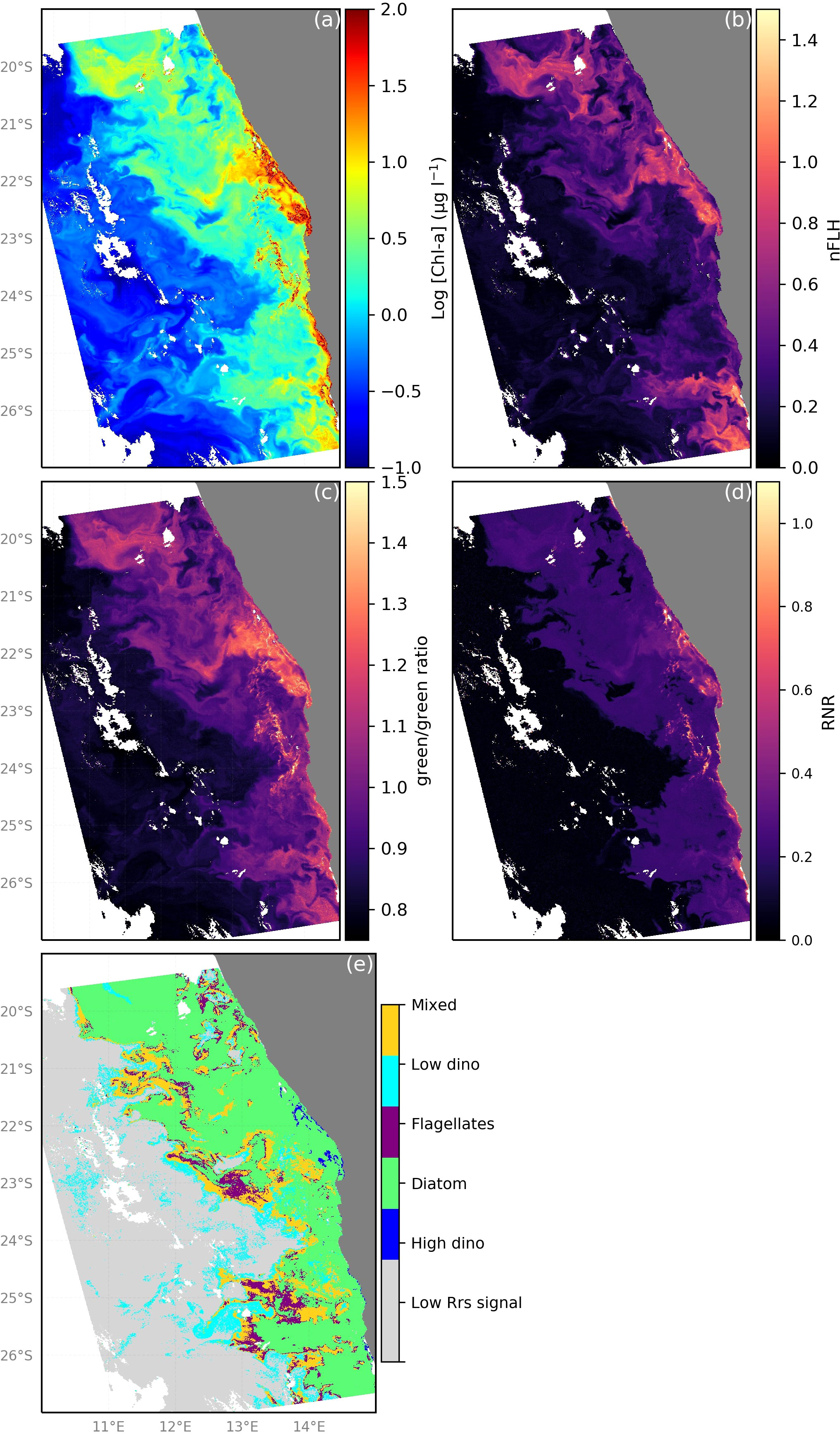
Figure 10 Demonstration of phytoplankton group dominance classification by the proposed ocean colour remote sensing algorithm for phytoplankton community from MODIS-Aqua observations for 11 March 2019 in the nBUS. (A) [Chl-a] distribution, (B) The observed nFLH, (C) green/green (Rrs547/Rrs531) band-ratio, (D) red/near-infrared (Rrs748/Rrs667) band-ratio and (E) application of the algorithm indicating the distribution of dominant phytoplankton groups in the nBUS.

4.4 Recognising algorithm limitations

4.4.1 Use of microscopy data

In situ phytoplankton data is a prerequisite for ocean colour algorithm development and validation for satellite remote sensing of phytoplankton from space. Inaccurate or incomplete in situ data undermines our ability to correctly associate optical signatures to cells that aren’t identified and may therefore lead to erroneous assignment of optical signatures to other phytoplankton groups, making accurate in situ measurements a scientific priority for increasing the accuracy and confidence of remote sensing and model development. Techniques such as microscopy are traditionally used in field observations for phytoplankton enumeration and taxonomic identification, providing valuable information for studying the diversity of phytoplankton taxa for assessing ecosystem health and balance, environmental monitoring and conservation, climatology and aiding aquaculture and fisheries industries with HABs detection among others (Anderson and Throndsen, 2004; Louw et al., 2017). Microscopic cell count techniques are particularly useful in that they provide identification of cells to species level. Although phytoplankton community information can be derived from these techniques, they have their limitations. For instance, analysis is dependent on highly trained and skilled people with thorough taxonomic expertise; these methods can be expensive, labour-intensive, time consuming, and may produce low precision unless a very large number of cells are counted (Anderson and Throndsen, 2004). Differential preservation of cells can lead to preferential cell loss and can thus introduce bias to sample classification (Williams et al., 2016). The use of preservatives greatly affects the observed community composition depending on which preservative is used [e.g. Lugol’s solution (either acidic or neutral) or formalin)] and for how long the samples were stored prior to analysis (Williams et al., 2016). For instance, armoured dinoflagellates are well preserved in all types of Lugols for up to 8 months whereas unarmoured dinoflagellates are only well preserved in acid Lugols for the same period. Microflagellates and diatoms are well preserved in acid Lugols (3 months and ~4 months respectively), while diatoms can also be stored in neutral Lugols (up to 2 months). Coccolithophores on the other hand are poorly preserved in acid Lugols and instead require neutral Lugols (2 weeks) (Williams et al., 2016). Phytoplankton samples from cruise campaigns in the current study were preserved in acidified (Meteor M153) and neutral (RGNO2019) Lugol’s solutions and analysed within 3 months of sampling. As such, coccolithophores may be misrepresented in both samples due to preferential preservation, this in addition to their small size which makes them harder to enumerate. Dinoflagellates (armoured and naked), diatoms and flagellates on the other hand are more likely to be well represented as they are generally well preserved in acidic Lugols even 225 days after sampling as opposed to the neutral Lugols with optimum preservation of samples for 28 days (Williams et al., 2016). In this regard, samples preserved in neutral lugol solution from the RGNO2019 cruise that were analysed after a month (but within 3 months) may be underrepresenting some of these groups (i.e. diatoms, flagellates, coccolithophores). Furthermore, smaller (picophytoplankton) and fragile cells are not easy to identify and quantify; as a result they may be under-represented. Indeed, the absence of an occurrence of coccolithophore dominance in this study may be due to their small size (making them harder to identify and enumerate) together with a poor ability to adequately preserve them in Lugols solution (Williams et al., 2016). Finally, interpersonal differences from data analysed in different laboratories may also undermine the precision of microscopic analyses. Identification of pigment markers of phytoplankton groups using high-performance liquid chromatography (HPLC) has been adopted as an alternative proxy for phytoplankton community analysis (Kheireddine et al., 2017; Kramer et al., 2020). This method has some advantages against microscopic analysis such as being highly reproducible and allowing the quantification and identification of smaller and more fragile cells, including cells that would normally be degraded by sample preservation with Lugols (Paul et al., 2021; Flander-Putrle et al., 2022). Advancements in the classification of phytoplankton groups has been made possible with the aid of specialised computer software such as CHEMTAX, which facilitates the classification of phytoplankton groups by means of pigment-to-Chl-a ratios (Mackey et al., 1996). However, pigment analysis is not able to provide the same level of detail as microscopy as they are not able to identify individual phytoplankton species. Also, similarities in photosynthetic pigments across multiple taxa make it difficult to distinguish different groups with confidence. Arguably, the future of phytoplankton enumeration lies within the realm of imaging with in situ cameras, holographic cameras and imaging flow cytometry. Although not without their own set of challenges (Giering et al., 2020), these approaches can generate images used to derive concentration and biodiversity information, as well as organism-specific size and shape (Boss et al., 2022). Given the strengths and weaknesses of all the various approaches, it is clear that no one technique can be considered the holy grail for phytoplankton community analysis and it is generally recommended that different techniques are integrated in order to provide a more comprehensive analysis of phytoplankton communities.

4.4.2 Limited datasets for development and validation

Although there was arguably an adequate sample size for stations with diatom dominance (n = 37) to allow this phytoplankton group to be more robustly characterised and partitioned into two sets of independent training (n=30) and validation (n=7), the number of matchup stations observing dominance of HB dinoflagellates (n=3), LB dinoflagellates (n=10), flagellates (n=11) and mixed phytoplankton community (n=13) were small. The qualitative nature of our algorithm only allows an indication of the dominance of one group in the presence of others and does not estimate the relative composition of each group nor the abundance of each group. It is recognised that these small data sets (which are further constrained by the necessity for satellite matchups in a region that is characterised by a persistent stratocumulus cloud deck) severely limit the robustness of the algorithm being developed. The authors are nonetheless committed to working with currently available and accessible data to explore the expansion of this data set for the purposes of validation of the existing algorithm and for future refinement with improved statistics as more data becomes available over time. In spite of the recognised limitations, it is clear that there is a dire need for such an algorithm and that the one proposed here provides a good first approach that can be applied retrospectively to 20 years of ocean colour data for important investigations that characterise the distribution patterns, phenology and trends of key phytoplankton groups in the region.

5 Conclusions

In the majority of the studies of community structure dynamics in the nBUS to date, microscopy has been the most commonly used technique for identifying phytoplankton distribution (Hansen et al., 2014; Dijerenge, 2015; Barlow et al., 2018) and environmental monitoring (Louw et al., 2017; Matlakala, 2019), although some studies used a combination of microscopy and pigment analysis (Barlow et al., 2018), with the limitations of both being clear. Satellite-based remote sensing of ocean colour is the only observational capability that can provide synoptic views of upper ocean phytoplankton characteristics at high spatial and temporal resolution (~1 km, ~daily) and a high temporal extent (global scales, for years to decades). It is thus important that we maximise the value of remote sensing observations by developing ecosystem-appropriate, well characterised products. This study takes advantage of unique spectral features (reflectance, reflectance ratios and spectral band difference) of oceanic waters dominated by various phytoplankton groups to create an ocean colour remote sensing algorithm for phytoplankton classification. Our future work will focus on acquiring additional in situ data for improvement and validation of the algorithm while venturing into discrimination of bloom types (e.g. non-HABs from HABs of diatoms of Pseudo-nitzschia species and dinoflagellates) and the detection of other key species (e.g. coccolithophores). Despite its limitations, the algorithm has enormous potential for mapping the distribution and phenology of phytoplankton groups on an unprecedented spatial and temporal scale in the nBUS. The intention is for this algorithm to be used for environmental monitoring of these phytoplankton types to better understand their spatial and temporal dynamics and environmental controls. In addition, application to the 20-year MODIS-aqua observation time series will allow an investigation of possible trends in community structure adjustments with important ecosystem implications for ocean-atmosphere exchange and energy transfer in support of the fisheries and aquaculture industries of Namibia.

Data availability statement

Publicly available datasets were analysed in this study. This data can be found here: The MODIS-Aqua data can be found at NASA’s ocean colour website https://oceancolor.gsfc.nasa.gov/. The MERIS data can be accessed through the MERIS catalogue and inventory (MERCI, http://meris-ds.eo.esa.int/oads/access/). The OLCI data can be found at the Copernicus online data access website (CODA, https://coda.eumetsat.int/). Phytoplankton counts and chlorophyll-a data can be accessed on the publicly available and accessible Pangaea database website at https://www.pangaea.de/.

Author contributions

The authors confirm their contribution to the manuscript as follows: Conceptualization: ST; MS. Methodology: MS; ST; TM. Data acquisition: TM; MS; ST; DL; BM; RK. Data curation: TM. Visualization (figures): TM. Formal analysis: TM; MS; ST. Manuscript 1st draft: TM. Supervision: ST; MS. Reviewing & editing: TM; MS; ST; BM; RK. Project administration: ST; MS. Funding acquisition: ST. All authors read, edited and approved the final version of the manuscript.

Funding

This research was supported as part of the Alliance for Collaboration on Climate and Earth Systems Science (ACCESS)-funded PLankton in a coupled oceAn-aTmOsphere system (PLATO) project by the National Research Foundation (NRF, South Africa, Grant No 114691) and the Council for Scientific and Industrial Research (CSIR, South Africa) through its Southern Ocean Carbon-Climate Observatory (SOCCO) programme funded by the Department of Science and Innovation (DSI, South Africa) and the parliamentary grant (SNA2011112600001). BM and RK as well as the use of the RV Meteor were funded by a grant from the Federal Ministry of Education and Research in Germany (FKZ 03F0797C).

Acknowledgments

We are grateful to Norbert Wasmund and Lebogang M. Matlakala for providing additional microscopy cell counts and [Chl-a] data. We would like to thank Kurt Hanselmann and colleagues at the National Marine Information and Research Centre (NatMIRC) for the RGNO2019 cruise organization and invaluable laboratory support. We thank Werner Ekau for organizing the Meteor M153 cruise that formed part of the Trophic TRAnsfer eFFICency in the Benguela Current (TRAFFIC) project.

Conflict of interest

The authors declare that the research was conducted in the absence of any commercial or financial relationships that could be construed as a potential conflict of interest.

Publisher’s note

All claims expressed in this article are solely those of the authors and do not necessarily represent those of their affiliated organizations, or those of the publisher, the editors and the reviewers. Any product that may be evaluated in this article, or claim that may be made by its manufacturer, is not guaranteed or endorsed by the publisher.

Supplementary material

The Supplementary Material for this article can be found online at: https://www.frontiersin.org/articles/10.3389/fmars.2023.1118226/full#supplementary-material

References

Agawin N. S. R., Rabouille S., Veldhuis M. J.W., Servatius L., Hol S., van Overzee M. J., et al. (2007). Competition and facilitation between unicellular nitrogen-fixing cyanobacteria and non – nitrogen-fixing phytoplankton species. Limnology Oceanography 52 (5), 2233–2248. doi: 10.4319/lo.2007.52.5.2233

CrossRef Full Text | Google Scholar

Aguirre-Gomez R., Weeks A. R., Boxshall S. R. (2001). The identification of phytoplankton pigments from absorption spectra. Int. J. Remote Sens. 22, 315–338. doi: 10.1080/014311601449952

CrossRef Full Text | Google Scholar

Aiken J., Fishwick J. R., Lavender S. J., Moore G. F., Sessions H., Bernard S., et al. (2007). Validation of MERIS reflectance and chlorophyll during the BENCAL cruise October 2002: Preliminary validation of new demonstration products for phytoplankton functional types and photosynthetic parameters. Int. J. Remote Sens. 28 (3–4), 497–516. doi: 10.1080/01431160600821036

CrossRef Full Text | Google Scholar

Allison E. H., Perry A. L., Badjeck M., Adger W. N., Brown K., Halls A. S., et al. (2009). Vulnerability of national economies to the impacts of climate change on fisheries. Fish Fisheries 10, 173–196. doi: 10.1111/j.1467-2979.2008.00310.x

CrossRef Full Text | Google Scholar

Anderson P., Throndsen J. (2004). ‘Estimating Cell numbers’, in Manual on Harmful Marine Microalgae. 2nd edition. Paris France: UNESCO p. 770. doi: 10.25607/OBP-1370

CrossRef Full Text | Google Scholar

Archer S. D., Widdicombe C. E., Tarran G. A., Rees A. P., Burkill P. H.. (2001). Production and turnover of particulate dimethylsulphoniopropionate during a coccolithophore bloom in the northern North Sea. Aquat. Microbial Ecol. 24, 225–241. doi: 10.3354/ame024225

CrossRef Full Text | Google Scholar

Arrigo K. R., Robinson D. H., Worthen D. L., Dunbar R. B., Ditullio G. R., Vanwoert M., et al. (1999). Phytoplankton community structure and the drawdown of nutrients and CO 2 in the Southern Ocean. Science 283, 365–368. doi: 10.1126/science.283.5400.365

CrossRef Full Text | Google Scholar

Bailey S. W., Werdell P. J. (2006). A multi-sensor approach for the on-orbit validation of ocean color satellite data products. Remote Sens. Environ. 102 (1–2), 12–23. doi: 10.1016/j.rse.2006.01.015

CrossRef Full Text | Google Scholar

Barlow R., Lamont T., Louw D., Gibberd M. J., Airs R., van der Plas A. (2018). Environmental influence on phytoplankton communities in the northern Benguela ecosystem. Afr. J. Mar. Sci. 40 (4), 355–370. doi: 10.2989/1814232X.2018.1531785

CrossRef Full Text | Google Scholar

Bernard S., Balt C., Pitcher G., Probyn T., Fawcett A., Du Randt A.. (2005). “The use of MERIS for harmful algal bloom monitoring in the Southern Benguela,” in Proceedings of the MERIS (A)A TSR workshop. Ed. Sawaya-Lacoste H. (Fracati, Italy: ESA Publ. Division), 1–7.

Google Scholar

Bestion E., Haegeman B., Codesal A. S., Garreau A., Huet M., Barton S., et al. (2021). Phytoplankton biodiversity is more important for ecosystem functioning in highly variable thermal environments. PNAS 118 (35), 1–10. doi: 10.1073/pnas.2019591118

CrossRef Full Text | Google Scholar

Boss E., Waite A. M., Karstensen J., Trull T., Muller-karger F., Sosik H. M., et al. (2022). Recommendations for plankton measurements on oceanSITES moorings with relevance to other observing sites. Front. Mar. Sci. 9 (July). doi: 10.3389/fmars.2022.929436

CrossRef Full Text | Google Scholar

Brewin R. J. W., Sathyendranath S., Jackson T., Barlow R., Brotas V., Airs R., et al. (2015). Influence of light in the mixed-layer on the parameters of a three-component model of phytoplankton size class. Remote Sens. Environment. Elsevier Inc. 168, 437–450. doi: 10.1016/j.rse.2015.07.004

CrossRef Full Text | Google Scholar

Brownlee C., Taylor A. R. (2002). “Algal calcification and silification,” in Encyclopedia of life sciences (Macmillan Publishers Ltd, Nature Publishing Group).

Google Scholar

Caldeira K., Duffy P. B. (2000). The role of the Southern Ocean in uptake and storage of anthropogenic carbon dioxide. Science 287, 620–623. doi: 10.1126/science.287.5453.620

CrossRef Full Text | Google Scholar

Carr M. (2002). Estimation of potential productivity in Eastern Boundary Currents using remote sensing. Deep-Sea Res. II 49, 59–80. doi: 10.1016/S0967-0645(01)00094-7

CrossRef Full Text | Google Scholar

Carr M., Kearns E. J. (2003). Production regimes in four Eastern Boundary Current systems. Deep-Sea Res. II 50, 3199–3221. doi: 10.1016/j.dsr2.2003.07.015

CrossRef Full Text | Google Scholar

Charlson R. J., Lovelock J. E., Andreae M. O., Warren S. G.. (1987). Oceanic phytoplankton, atmospheric sulphur, cloud albedo and climate. Nature 326 (6114), 655–661. doi: 10.1038/326655a0

CrossRef Full Text | Google Scholar

Chavez F. P., Messié M. (2009). Progress in oceanography: A comparison of eastern boundary upwelling ecosystems. Prog. Oceanography. Elsevier Ltd 83 (1–4), 80–96. doi: 10.1016/j.pocean.2009.07.032

CrossRef Full Text | Google Scholar

Coble P. G. (2013). “Colored dissolved organic matter in seawater,” in Subsea optics and imaging. (Florida: Woodhead Publishing Limited), 98–118. doi: 10.1533/9780857093523.2.98

CrossRef Full Text | Google Scholar

Cury P., Shannon L. (2004). Regime shifts in upwelling ecosystems: observed changes and possible mechanisms in the northern and Southern Benguela. Prog. Oceanography 60, 223–243. doi: 10.1016/j.pocean.2004.02.007

CrossRef Full Text | Google Scholar

Dermastia T. T., Ara S. D., Dolenc J., Mozetiˇ P.. (2022). Toxicity of the diatom genus Pseudo-nitzschia (Bacillariophyceae): insights from toxicity tests and genetic screening in the Northern Adriatic Sea. Toxins 14 (60), 1–17. doi: 10.3390/toxins14010060

CrossRef Full Text | Google Scholar

Dijerenge K. J. (2015). Analysis of marine biotoxins: Paralytic and Lipophilic Shellfish Toxins in Mussels (Mytilus galloprovincialis) along the Namibian Coastline, University of Namibia. (Namibia: University of Namibia). https://repository.unam.edu.na/handle/11070/1466.

Google Scholar

Dogliotti A. I., Schloss I. R., Almandoz G. O., Gagliardini D. A. (2009). Evaluation of SeaWiFS and MODIS chlorophyll-a products in the Argentinean Patagonian Continental Shelf (38° S-55° S). Int. J. Remote Sens. 30 (1), 251–273. doi: 10.1080/01431160802311133

CrossRef Full Text | Google Scholar

D’Sa E. J., Kim H. (2017). Surface gradients in dissolved organic matter absorption and fluorescence properties along the New Zealand sector of the Southern Ocean. Front. Mar. Sci. 4 (21), 1–14. doi: 10.3389/fmars.2017.00021

CrossRef Full Text | Google Scholar

Duncombe Rae C. M. (2005). A demonstration of the hydrographic partition of the Benguela upwelling ecosystem at 26° 40 ‘ S. Afr. J. Mar. Sci. 27 (3), 617–628. doi: 10.2989/18142320509504122

CrossRef Full Text | Google Scholar

Evers-King H. (2014). Phytoplankton community structure determined through remote sensing and in situ optical measurements. PhD thesis. (South Africa: University of Cape Town).

Google Scholar

Fawcett A., Pitcher G. C., Bernard S., Cembella A. D., Kudela R. M. (2007). Contrasting wind patterns and toxigenic phytoplankton in the Southern Benguela upwelling system. Mar. Ecol. Prog. Ser. 348, 19–31. doi: 10.3354/meps07027

CrossRef Full Text | Google Scholar

Field C. B., Behrenfeld M. J., Randerson J. T., Falkowski P. (1998). Primary production of the biosphere : integrating terrestrial and oceanic components. Science 281, 237–241. doi: 10.1126/science.281.5374.237

CrossRef Full Text | Google Scholar

Flander-Putrle V., Francé J., Mozetič P. (2022). Phytoplankton pigments reveal size structure and interannual variability of the coastal phytoplankton community (Adriatic sea). Water 14 (1), 23. doi: 10.3390/w14010023

CrossRef Full Text | Google Scholar

Gai F. F., Hedemand C. K., Louw D. C., Grobler K., Krock B., Moestrup Ø., et al. (2018). ‘Morphological, molecular and toxigenic characteristics of Namibian Pseudo-nitzschia species – including Pseudo-nitzschia bucculenta sp. nov. Harmful Algae 76 (May), 80–95. doi: 10.1016/j.hal.2018.05.003

CrossRef Full Text | Google Scholar

Giering S. L. C., Cavan E. L., Basedow S. L., Briggs N., Burd A. B., Darroch L. J., et al. (2020). Sinking organic particles in the ocean–flux estimates from in situ optical devices. Front. Mar. Sci. 6. doi: 10.3389/fmars.2019.00834

CrossRef Full Text | Google Scholar

Gilerson A., Zhou J., Hlaing S., Ioannou I., Schalles J., Gross B., et al. (2007). Fluorescence component in the reflectance spectra from coastal waters. Dependence on water composition. Optics Express 15 (24), 15702–15721. doi: 10.1029/2002GL016185

CrossRef Full Text | Google Scholar

Gordon H. R. (1979). Diffuse reflectance of the ocean: the theory of its augmentation by chlorophyll a fluorescence at 685 nm. Appl. Optics 18 (8), 1161. doi: 10.1364/ao.18.001161

CrossRef Full Text | Google Scholar

Hansen A., Ohde T., Wasmund N. (2014). Succession of micro- and nanoplankton groups in ageing upwelled waters off Namibia. J. Mar. Syst. 140 (PB), 130–137. doi: 10.1016/j.jmarsys.2014.05.003

CrossRef Full Text | Google Scholar

Hirata T., Hardman-Mountford N. J., Brewin R. J. W., Aiken J., Barlow R., Suzuki K., et al. (2011). Synoptic relationships between surface Chlorophyll- a and diagnostic pigments specific to phytoplankton functional types. Biogeosciences 8, 311–327. doi: 10.5194/bg-8-311-2011

CrossRef Full Text | Google Scholar

Hoagland P., Anderson D. M., Kaoru Y., White A. W. (2002). The economic effects of harmful algal blooms in the United States : estimates, assessment issues, and information needs. Estuaries 25 (4), 819–837. doi: 10.1007/BF02804908

CrossRef Full Text | Google Scholar

Hu C., Muller-karger F. E., Taylor J. C., Carder K. L., Kelble C., Johns E, et al. (2005). Red tide detection and tracing using MODIS fluorescence data : A regional example in SW Florida coastal waters. Remote Sens. Environ. 97, 311–321. doi: 10.1016/j.rse.2005.05.013

CrossRef Full Text | Google Scholar

Hu C., Lee Z., Franz B. (2012). Chlorophyll a algorithms for oligotrophic oceans: A novel approach based on three-band reflectance difference. J. Geophysical Research: Oceans 117 (1), 1–25. doi: 10.1029/2011JC007395

CrossRef Full Text | Google Scholar

Hutchings L., van der Lingen C. D., Shannon L. J., Crawford R. J. M., Verheye H. M. S., Bartholomae C. H., et al. (2009). The Benguela Current: An ecosystem of four components. Prog. Oceanography 83 (1–4), 15–32. doi: 10.1016/j.pocean.2009.07.046

CrossRef Full Text | Google Scholar

Isada T., Abe H., Kasai H., Nakaoka M.. (2021). Dynamics of nutrients and colored dissolved organic matter absorption in a wetland-influenced subarctic coastal region of Northeastern Japan: contributions from mariculture and eelgrass meadows. Front. Mar. Sci. 8 (711832), 1–19. doi: 10.3389/fmars.2021.711832

CrossRef Full Text | Google Scholar

Kampf J., Chapman P. (2016). “The benguela current upwelling system,” in Upwelling systems of the world. (Switzerland: Springer), 251–314. doi: 10.1007/978-3-319-42524-5

CrossRef Full Text | Google Scholar

Keller M. D. (1989). Dimethyl sulfide production and marine phytoplankton: the importance of species composition and cell size. Biol. Oceanography 6, 375–382. doi: 10.1080/01965581.1988.10749540

CrossRef Full Text | Google Scholar

Kheireddine M., Ouhssain M., Claustre H., Uitz J., Gentili B., Jones B. H.. (2017). Assessing pigment-based phytoplankton community distributions in the Red Sea. Front. Mar. Sci. 4 (MAY). doi: 10.3389/fmars.2017.00132

CrossRef Full Text | Google Scholar

Kramer S. J., Siegel D. A., Graff J. R. (2020). Phytoplankton community composition determined from co-variability among phytoplankton pigments from the NAAMES field campaign. Front. Mar. Sci. 7 (April). doi: 10.3389/fmars.2020.00215

CrossRef Full Text | Google Scholar

Kritten L., Preusker R., Fischer J. (2020). A new retrieval of sun-induced chlorophyll fluorescence in water from ocean colour measurements applied on OLCI L-1b and L-2. Remote Sens. 12 (23), 1–24. doi: 10.3390/rs12233949

CrossRef Full Text | Google Scholar

Kruk C., Peeters E. T. H. M., Nes Van Huszar E. H. V. L. M., Costa L. S., Scheffer M.. (2011). Phytoplankton community composition can be predicted best in terms of morphological groups. Limnology Oceanography 56 (1), 110–118. doi: 10.4319/lo.2011.56.1.0110

CrossRef Full Text | Google Scholar

Kwak I., Park Y. (2020). Food chains and food webs in aquatic ecosystems. Appl. Sci. 10 (5012), 1–5. doi: 10.3390/app10145012

CrossRef Full Text | Google Scholar

Lachkar Z., Gruber N. (2012). A comparative study of biological production in eastern boundary upwelling systems using an artificial neural network. Biogeosciences 9, 293–308. doi: 10.5194/bg-9-293-2012

CrossRef Full Text | Google Scholar

Laiolo L., Matear R., Soja-wo M., Suggett D. J., Hughes D. J., Baird M. E., et al. (2021). Modelling the impact of phytoplankton cell size and abundance on inherent optical properties (IOPs ) and a remotely sensed chlorophyll- a product. J. Mar. Syst. 213, 1–12. doi: 10.1016/j.jmarsys.2020.103460

CrossRef Full Text | Google Scholar

Lamont T., Barlow R. G., Brewin R. J. W. (2019). Long - term trends in phytoplankton chlorophyll a and size structure in the benguela upwelling system. J. Geophysical Research: Oceans 51 (10), 1170–1195. doi: 10.1029/2018JC014334

CrossRef Full Text | Google Scholar

Lamont T., García-Reyes M., Bograd S. J., van der Lingen C. D., Sydeman W. J. (2018). Upwelling indices for comparative ecosystem studies: Variability in the Benguela Upwelling System. J. Mar. Syst. 188, 3–16. doi: 10.1016/j.jmarsys.2017.05.007

CrossRef Full Text | Google Scholar

Lass H. U., Mohrholz V. (2008). On the interaction between the subtropical gyre and the Subtropical Cell on the shelf of the SE Atlantic. J. Mar. Systems. 74 (1–2), 1–43. doi: 10.1016/j.jmarsys.2007.09.008

CrossRef Full Text | Google Scholar

Letelier R. M., Abbott M. R. (1996). An analysis of chlorophyll fluorescence algorithms for the moderate resolution imaging spectrometer (MODIS). Remote Sens. Environ. 58 (2), 215–223. doi: 10.1016/S0034-4257(96)00073-9

CrossRef Full Text | Google Scholar

Lett C., Veitch J., van der Lingen C. D., Hutchings L. (2007). Assessment of an environmental barrier to transport of ichthyoplankton from the southern to the northern Benguela ecosystems. Mar. Ecol. Prog. Ser. 347, 247–259. doi: 10.3354/meps06982

CrossRef Full Text | Google Scholar

Lizotte M., Levasseur M., Law C. S., Walker C. F., Safi K. A., Marriner A. (2017). Dimethylsulfoniopropionate (DMSP) and dimethyl sulfide (DMS) cycling across contrasting biological hotspots of the New Zealand subtropical front. Ocean Sci. 13, 961–982. doi: 10.5194/os-13-961-2017

CrossRef Full Text | Google Scholar

Louw D. C., Doucette G. J., Voges E. (2017). Annual patterns, distribution and long-term trends of Pseudo-nitzschia species in the northern Benguela upwelling system. J. Plankton Res. 39 (1), 35–47. doi: 10.1093/plankt/fbw079

CrossRef Full Text | Google Scholar

Louw D. C., Plas A. K., Van Der Mohrholz V., Wasmund N., Junker T., Eggert A.. (2016). Seasonal and interannual phytoplankton dynamics and forcing mechanisms in the Northern Benguela upwelling system. J. Mar. Systems. 157, 124–134. doi: 10.1016/j.jmarsys.2016.01.009

CrossRef Full Text | Google Scholar

Mackey M. D., Mackey D. J., Higgins H. W., Wright S. W. (1996). CHEMTAX - A program for estimating class abundances from chemical markers: Application to HPLC measurements of phytoplankton. Mar. Ecol. Prog. Ser. 144 (1–3), 265–283. doi: 10.3354/meps144265

CrossRef Full Text | Google Scholar

Mao Z., Stuart V., Pan D., Chen J., Gong F., Huang H., et al. (2010). Effects of phytoplankton species composition on absorption spectra and modeled hyperspectral reflectance. Ecol. Informatics. 5 (5), 359–366. doi: 10.1016/j.ecoinf.2010.04.004

CrossRef Full Text | Google Scholar

Matlakala M. L. (2019). Seasonal characteristics of phytoplankton bloom phenology in the northern Benguela Upwelling System. (Cape Town, Rondebosch, South Africa: University of Cape Town).

Google Scholar

Mayer K. J., Wang X., Santander M. V, Mitts B. A., Sauer J. S., Sultana C. M., et al. (2020). Secondary marine aerosol plays a dominant role over primary sea spray aerosol in cloud formation. ACS Cent. Sci. 6 (12), 2259–2266. doi: 10.1021/acscentsci.0c00793

CrossRef Full Text | Google Scholar

Mcclelland H. L. O., Barbarin N., Beaufort L., Hermoso M., Ferretti P., Greaves M., et al. (2016). Calcification response of a key phytoplankton family to millennial- scale environmental change. Nat. Sci. Rep. Nat. Publishing Group 6, 1–11. doi: 10.1038/srep34263

CrossRef Full Text | Google Scholar

Mohrholz V., Eggert A., Junker T., Nausch G., Ohde T., Schmidt M.. (2014). Cross shelf hydrographic and hydrochemical conditions and their short term variability at the northern Benguela during a normal upwelling season. J. Mar. Systems. 140 (PB), 92–110. doi: 10.1016/j.jmarsys.2014.04.019

CrossRef Full Text | Google Scholar

Morel A., Claustre H., Gentili B. (2010). The most oligotrophic subtropical zones of the global ocean: Similarities and differences in terms of chlorophyll and yellow substance. Biogeosciences 7 (10), 3139–3151. doi: 10.5194/bg-7-3139-2010

CrossRef Full Text | Google Scholar

Moutier W., Thomalla S. J., Bernard S., Wind G., Ryan-keogh T. J., Smith M. E. (2019). Evaluation of chlorophyll-a and POC MODIS aqua products in the southern ocean. Remote Sens. 11, 1–18. doi: 10.3390/rs11151793

CrossRef Full Text | Google Scholar

Ohde T., Dadou I. (2018). Seasonal and annual variability of coastal sulphur plumes in the northern Benguela upwelling system. PloS One 13 (2), 1–33. doi: 10.1371/journal.pone.0192140

CrossRef Full Text | Google Scholar

O’Reilly J. E., Maritorena S., Mitchell B. G., Siegel D. A., Carder K. L., Garver S. A., et al. (1998). Ocean color chlorophyll algorithms for SeaWiFS. J. Geophysical Res. 103 (Cll), 24937–24953. doi: 10.1029/98JC02160

CrossRef Full Text | Google Scholar

O’Reilly J. (2000). “Ocean Color Chlorophyll-a Algorithm for SeaWiFS, OC2, and OC4: SeaWiFS Postlaunch Technical Report Series,”In: Hooker S. B., Firestone R. Eds., Volume 11, SeaWiFS Postlaunch Calibration and Validation Analyses Version 4, Part 3, NASA Goddard Space Flight Center, Greenbelt, 9–23.

Google Scholar

Otero J., Álvarez-salgado X. A., Bode A. (2020). Phytoplankton diversity effect on ecosystem functioning in a coastal upwelling system. Front. Mar. Sci. 7. doi: 10.3389/fmars.2020.592255

CrossRef Full Text | Google Scholar

Paul M., Velappan M. N., Nanappan U., Gopinath V., Velloth R. T., Rajendran A., et al. (2021). Characterization of phytoplankton size-structure based productivity, pigment complexes (HPLC/CHEMTAX) and species composition in the Cochin estuary (southwest coast of India): special emphasis on diatoms. Oceanologia. 63 (4), 463–481. doi: 10.1016/j.oceano.2021.05.004

CrossRef Full Text | Google Scholar

Pei S., Laws E. A., Zhang H., Ye S., Yuan H., Liu H. (2017). Patchiness of phytoplankton and primary production in Liaodong Bay, China. PloS One 12 (2), 1–14. doi: 10.1371/journal.pone.0173067

CrossRef Full Text | Google Scholar

Pollard R. T., Salter I., Sanders R. J., Lucas M. I., Moore C. M., Mills R. A., et al. (2009). Southern Ocean deep-water carbon export enhanced by natural iron fertilization. Nature 457, 14–18. doi: 10.1038/nature07716

CrossRef Full Text | Google Scholar

Polonsky A. B., Serebrennikov A. N. (2020). On the change in the sea surface temperature in the Benguela upwelling region: part II. Long-term tendencies. Atmospheric Ocean Phys. 56 (9), 970–978. doi: 10.1134/S0001433820090200

CrossRef Full Text | Google Scholar

Riebesell U., Rost B. (2004). “Coccolithophores and the biological pump: responses to environmental changes,” in Coccolithophores: from molecular processes to global impact. Eds. Young J. R., Thierstein H. R. (Berlin: Springer), 99–125.

Google Scholar

Rouault M., Illig S., Lübbecke J., Koungue R. A. I. (2018). Origin, development and demise of the 2010 – 2011 Benguela Niño. J. Mar. Systems. 188 (November 2016), 39–48. doi: 10.1016/j.jmarsys.2017.07.007

CrossRef Full Text | Google Scholar

Schalles J. F. (2006). “Optical remote sensing techniques to estimate phytoplankton chlorophyll a concentrations in coastal waters with varying suspended matter and cdom concentrations,” in Remote sensing of aquatic coastal ecosystem processes. (Dordrecht: Springer), 27–79.

Google Scholar

Scheinin M., Asmala E. (2020). Ubiquitous patchiness in chlorophyll a concentration in coastal archipelago of Baltic Sea. Front. Mar. Sci. 7 (July). doi: 10.3389/fmars.2020.00563

CrossRef Full Text | Google Scholar

Shikwambana L., Kganyago M. (2022). Meteorological influence of mineral dust distribution over South-Western Africa deserts using reanalysis and satellite data. Front. Environ. Sci. 10 (June). doi: 10.3389/fenvs.2022.856438

CrossRef Full Text | Google Scholar

Shillington F., Reason C. J., Duncombe rae C., Florenchie P., Penven P. (2006). Large scale physical variability of the benguela current large marine ecosystem (BCLME). Large Mar. Ecosyst. 14, 15–30. doi: 10.1016/S1570-0461(06)80009-1

CrossRef Full Text | Google Scholar

Smetacek V. (1999). Diatoms and the ocean carbon cycle. Protist 150 (1), 25–32. doi: 10.1016/S1434-4610(99)70006-4

CrossRef Full Text | Google Scholar

Smith M. E., Bernard S. (2020). Satellite ocean color based harmful algal bloom indicators for aquaculture decision support in the Southern Benguela. Front. Mar. Sci. 7 (61). doi: 10.3389/fmars.2020.00061

CrossRef Full Text | Google Scholar

Smith M. E., Robertson Lain L., Bernard S. (2018). An optimized Chlorophyll a switching algorithm for MERIS and OLCI in phytoplankton-dominated waters. Remote Sens. Environ. 215 (January), 217–227. doi: 10.1016/j.rse.2018.06.002

CrossRef Full Text | Google Scholar

Soja-Wozniak M., Darecki M., Wojtasiewicz B. (2018). Laboratory measurements of remote sensing reflectance of selected phytoplankton species from the Baltic Sea. Oceanologia 60, 86–96. doi: 10.1016/j.oceano.2017.08.001

CrossRef Full Text | Google Scholar

Soja-Woźniak M., Laiolo L., Baird M. E., Matear R., Clementson L., Schroeder T., et al. (2020). Effect of phytoplankton community size structure on remote-sensing reflectance and chlorophyll a products. J. Mar. Syst. 211, 103400. doi: 10.1016/j.jmarsys.2020.103400

CrossRef Full Text | Google Scholar

Spirig R., Vogt R., Larsen J. A., Feigenwinter C., Wicki A., Franceschi J., et al. (2017). Probing the fog life cycles in the Namib desert. Bull. Am. Meteorological Soc. 100 (12), 2491–2508. doi: 10.1175/BAMS-D-18-0142.1

CrossRef Full Text | Google Scholar

Stefels J. (2000). Physiological aspects of the production and conversion of DMSP in marine algae and higher plants. J. Sea Res. 43 (3–4), 183–197. doi: 10.1016/S1385-1101(00)00030-7

CrossRef Full Text | Google Scholar

Stock C. A., John J. G., Rykaczewski R. R., Asch R. G., Cheung W. W. L., Dunne J. P., et al. (2017). Reconciling fisheries catch and ocean productivity. PNAS 1, 1441–1449. doi: 10.1073/pnas.1610238114

CrossRef Full Text | Google Scholar

Thuillier G., Herse M., Labs D., Foujols T., Peetermans W., Gillotay D., et al. (2003). The solar spectral irradiance from 200 to 2400 nm as measured by the SOLSPEC spectrometer from the ATLAS and EURECA missions. Solar Phys. 214 (1), 1–22. doi: 10.1023/A:1024048429145

CrossRef Full Text | Google Scholar

Tortell P. D., Payne C. D., Li Y., Trimborn S., Smith W. O., Riesselman C., et al. (2008). CO 2 sensitivity of Southern Ocean phytoplankton. Geophysical Res. Lett. 35, 1–5. doi: 10.1029/2007GL032583

CrossRef Full Text | Google Scholar

Uitz J., Claustre H., Morel A., Hooker S. B.. (2006). Vertical distribution of phytoplankton communities in open ocean : An assessment based on surface chlorophyll. J. Geophysical Res. 111 (1), 1–23. doi: 10.1029/2005JC003207

CrossRef Full Text | Google Scholar

Utermöhl H. (1958). Zur Vervollkommnung der quantitativen Phytoplankton-Methodik. Mitt. der Internationalen Vereinigung für Theoretische und Angewandte Limnologie 9 (1), 1–38. doi: 10.1080/05384680.1958.11904091

CrossRef Full Text | Google Scholar

Vaillancourt R. D., Brown C. W., Guillard R. R. L., Balch W. M. (2004). Light backscattering properties of marine phytoplankton : relationships to cell size, chemical composition and taxonomy. J. Plankton Res. 26 (2), 191–212. doi: 10.1093/plankt/fbh012

CrossRef Full Text | Google Scholar

Vidussi F., Clauster H., Manca B. B., Luchetta A., Marty J.-C. (2001). Phytoplankton pigment distribution in relation to upper thermocline circulation in the eastern Mediterranean Sea during winter. J. Geophysical Res. 106, 939–956. doi: 10.1029/1999JC000308

CrossRef Full Text | Google Scholar

Wasmund N. (2011a). Chlorophyll pigments from the Namibian upwelling system during Discovery 356, Leibniz Institute for Baltic Sea Research. doi: 10.1594/PANGAEA.773204

CrossRef Full Text | Google Scholar

Wasmund N. (2011b). Phytoplankton biomass from the Namibian upwelling system during Discovery 356, Leibniz Institute for Baltic Sea Research (Warnemünde: PANGAEA). doi: 10.1594/PANGAEA.773205

CrossRef Full Text | Google Scholar

Wasmund N. (2012). Phytoplankton measurements from the Namibian upwelling system during the Maria S. Merian cruise MSM 17/3, Leibniz Institute for Baltic Sea Research (Warnemünde: PANGAEA). doi: 10.1594/PANGAEA.779150

CrossRef Full Text | Google Scholar

Wasmund N. (2015a). Chlorophyll pigments from the Namibian upwelling system during Maria S. Merain cruise MSM17/3 (PANGAEA). doi: 10.1594/PANGAEA.843325

CrossRef Full Text | Google Scholar

Wasmund N. (2015b). Chlorophyll pigments from the Namibian upwelling system during Maria S. Merain cruise MSM18/4 (PANGAEA). doi: 10.1594/PANGAEA.843328

CrossRef Full Text | Google Scholar

Wasmund N. (2015c). Phytoplankton biomass from the Namibian upwelling system during Maria S. Merain cruise MSM18/4 (PANGAEA). doi: 10.1594/PANGAEA.843339

CrossRef Full Text | Google Scholar

Wasmund N., Nausch G., Hansen A. (2014). Phytoplankton succession in an isolated upwelled Benguela water body in relation to different initial nutrient conditions. J. Mar. Systems. 140 (1), 163–174. doi: 10.1016/j.jmarsys.2014.03.006

CrossRef Full Text | Google Scholar

Welschmeyer N. (1994). Fluorometric analysis of chlorophyll a in the presence of chlorophyll b and pheopigments. Limnology Oceanography 39 (8), 1985–1992. doi: 10.4319/lo.1994.39.8.1985

CrossRef Full Text | Google Scholar

Williams O. J., Beckett R. E., Maxwell D. L. (2016). Marine phytoplankton preservation with Lugol’s: a comparison of solutions. J. Appl. Phycology. J. Appl. Phycology 28 (3), 1705–1712. doi: 10.1007/s10811-015-0704-4

CrossRef Full Text | Google Scholar