 Spyros Spondylidis1*
 Marianna Giannoulaki2
 Athanassios Machias2
 Ioannis Batzakas1
 Konstantinos Topouzelis1
- 1Department of Marine Sciences, University of the Aegean, Mytilene, Greece
- 2Institute of Marine Biological Resources, Hellenic Center for Marine Research, Irakleion, Greece
Fish population spatial distribution data provide essential information for fleet monitoring and fishery spatial planning. Modern high resolution ocean color remote sensing sensors with daily temporal coverage can enable consistent monitoring of highly productive areas, giving insight in seasonal and yearly variations. Here is presented the methodology to monitor small pelagic fish spatial distribution by means of 500m resolution satellite data in a geographically and oceanographically complex area. Specifically, anchovy (Engraulis encrasicolus) and sardine (Sardina pilchardus) acoustic biomass data are modeled against environmental proxies obtained from the Sentinel-3 satellite mission. Three modeling techniques (Logistic Regression, Generalized Additive Models, Random Forest) were applied and validated against the in-situ measurements. The accuracy of anchovy presence detection peaked at 76% and for sardine at 78%. Additionally, the spatial distribution of the models’ output highlighted known fishing grounds. For anchovy, biomass modeling highlighted the importance of bathymetry, SST, and the distance from thermal fronts, whereas for sardine, bathymetry, CHL and chlorophyll fronts. The models are applied to a sample dataset to showcase a potential outcome of the proposed methodology and its spatial characteristics. Finally, the results are discussed and compared to other habitat studies and findings in the area.
1 Introduction
Remote sensing data provide invaluable tools for monitoring the marine and coastal environment. They help monitor the spread of oil spills, locate waste on beaches, map marine vegetation, quantify shoreline retreats, etc (Brekke and Solberg, 2005; Traganos et al., 2018; Apostolopoulos and Nikolakopoulos, 2021; Hu, 2021). They stand out from field data due to their spatial and temporal coverage and free access, making in-depth investigations time feasible. Recent studies and reports have shown that the commercial species in the Greek Seas and the Mediterranean are continuously overexploited bringing a steady decline in landings and the respective ecological impacts (Tsikliras et al., 2020; FAO, 2022). By these trends, monitoring the spatial distribution of fish populations holds particular importance for fisheries management authorities, which could also enable the integration of fisheries in marine spatial planning (Mazor et al., 2014; Baudron et al., 2020; Bellido et al., 2020).
Spatiotemporal monitoring of fish population distribution holds value in both academic and administrative practices. Relating climate data to fish spatial distribution changes can provide insight to the effects of climate change on marine biodiversity per region (Nye et al., 2009; Pinsky et al., 2020; Román-Palacios and Wiens, 2020). In the case of small pelagic fish in the Mediterranean Sea recent studies on future climate scenarios have reported mixed results on the level of impact (Gkanasos et al., 2021; Tsagarakis et al., 2022). Continuous monitoring the spatial distribution of the species in relation to environmental changes could add a beneficial dataset to this research field.
In their work Janßen et al., 2018 highlight that fish distribution monitoring is a key factor in the integration of fisheries in marine spatial planning. On the other hand, such info can be beneficiary to the economic sector as well, provided that it is integrated conscientiously. Such data can act as an advisory tool for the fishing fleets to maximize the catch by simultaneously reducing the costs due to targeted fishing without wasting expenses on fuel and man hours (Nair and Pillai, 2012).
One of the most widespread methods of locating and predicting fishing zones is multicriteria analysis modeling. In the Aegean, satellite-derived chlorophyll-a concentration (CHL) and Sea Surface Temperature (SST) have been useful in the identification of productivity hotspots, indicating that satellite-based monitoring can be used for the benefit of fisheries management Valavanis et al., 2004. Additionally, through satellite data oceanic formations can be extracted, which in many cases hold significant ecological importance. Mansor et al., 2001 used a multi-criteria model to predict potential fishing zones with SST and CHL input data. The model uses the SST to identify oceanic fronts and upwelling areas that signal the increased probability of creating a fishing zone. Other studies on Essential Fish Habitat (EFH) mapping focus on describing the geographical distribution of marine species with fishery data (Total Catch, CPUE, acoustic surveys etc.) and relevant oceanographic parameters, like temperature and trophic level, and geological i.e., bathymetry and substrate type (Valavanis et al., 2008).
It has been showcased that satellite data can be used successfully in fish population and habitat mapping. But most of the studies focus on a time snapshot of the current conditions (Valavanis et al., 2004; Giannoulaki et al., 2005; Bellido et al., 2008; Giannoulaki et al., 2008; Bonanno et al., 2014; Colloca et al., 2015). The marine environment though is both spatially and temporally variable due to seasonal and oceanographic changes or due to more long-term factors such as climate change. Furthermore, traditional methodologies are implemented with course resolution remote sensing data which, in most cases, are not sufficient for administrative and decision-making purposes (Janßen et al., 2018). Ocean color remote sensing has evolved in the past decade to the point that high resolution data are available on a daily basis. It is crucial now to explore these new technologies and how they can be used to provide continuous reliable information on fisheries and if they can be utilized to evolve current methodologies.
Higher resolution remote sensing data also contribute in finer oceanic circulation mapping, whose importance in fish spatial distribution modeling has been widely stated in both regional studies (Somarakis and Nikolioudakis, 2007; Tsoukali et al., 2019) and international ones (Godø et al., 2012; Arur et al., 2014; Kürten et al., 2019). Until now, fish spatial distribution studies and methodologies that use remote sensing data utilize lower resolution datasets (> 1km) from the Moderate Resolution Imaging Spectroradiometer (MODIS) and Sea-viewing Wide Field-of-view Sensor (SeaWiFS) (Zhang et al., 2017; Fauziyah et al., 2022). Higher resolution data, such as Sentinel-3, could provide more information on oceanic circulation and distinguish formations of a lower scale. The benefits of using finer resolution datasets on sub-mesoscale front detection have already been showcased with implementations on the MEdium Resolution Imaging Spectrometer (MERIS) (Miller et al., 2015), with a temporal coverage of 3 days. On the other hand, Sentinel-3’s Ocean and Land Color Instrument (OLCI) passes over an area between 1-1.5 days and would be more suitable for continuous monitoring.
This paper scopes to explore small pelagic fish distribution monitoring with the combined use of marine environmental proxies retrieved from high resolution satellite data and in-situ biomass data of anchovy (Engraulis encrasicolus) and sardine (Sardina pilchardus) from a 2-year acoustic survey. Sentinel-3 OLCI (300m resolution) and SLSTR (500m resolution) data are used along with extracted sub-mesoscale oceanic fronts and bathymetric information to model the spatial distribution of anchovy and sardine with the use of in-situ acoustic biomass data. The species’ presence is modeled with 3 classification models and the validation results are presented. Additionally, fish biomass was simulated directly through satellite data by a regression model. A full list of the abbreviations used in this paper is given in Supplementary Data Sheet 1.
2 Materials and methods
The developed methodology focuses on a 5-step process based on the flow chart in Figure 1. The first two steps are a) Data and b) Pre-processing, which target on data acquisition and data preparation for further analysis, including the oceanic front detection process that engulfs the satellite data analysis for (Sub) Mesoscale Front identification. The final two steps are c) Biomass Modeling, referring to modeling phase to retrieve fish spatial distribution and d) Validation of the methodology.
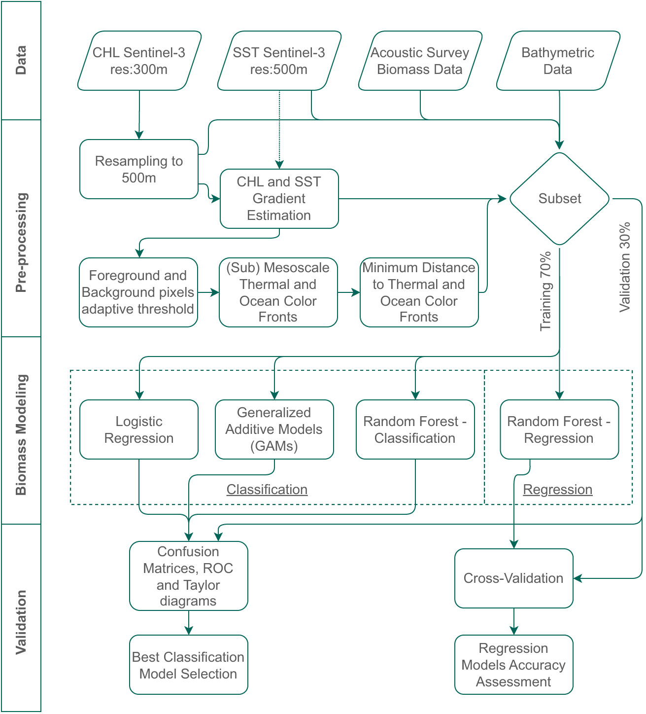
Figure 1 The 4-step methodology flow chart, describing intermediate procedures for a) Data, b) Pre-processing, c) Biomass Modeling and d) Validation.
2.1 Study area
The study area is the North Aegean Sea (Eastern Mediterranean), divided into the Thracian Sea (TS) and the Gulf of Thermaikos (GT) because of differences in topography and oceanographic characteristics (Figure 2). The North Aegean is connected to the Sea of Marmaras and the Black Sea through the Dardanelles and Bosphorus Straits. South of the Halkidiki peninsula, in a NE-SW direction, there is the North Aegean Trench with a maximum depth of 1600 m north of Lemnos Island (Lykousis et al., 2002). Five rivers flow in the Northern Aegean, Axios and Aliakmonas in the GT, Strymon in the Strymonikos Gulf, and Nestos and Evros in the Central and Eastern TS respectively.
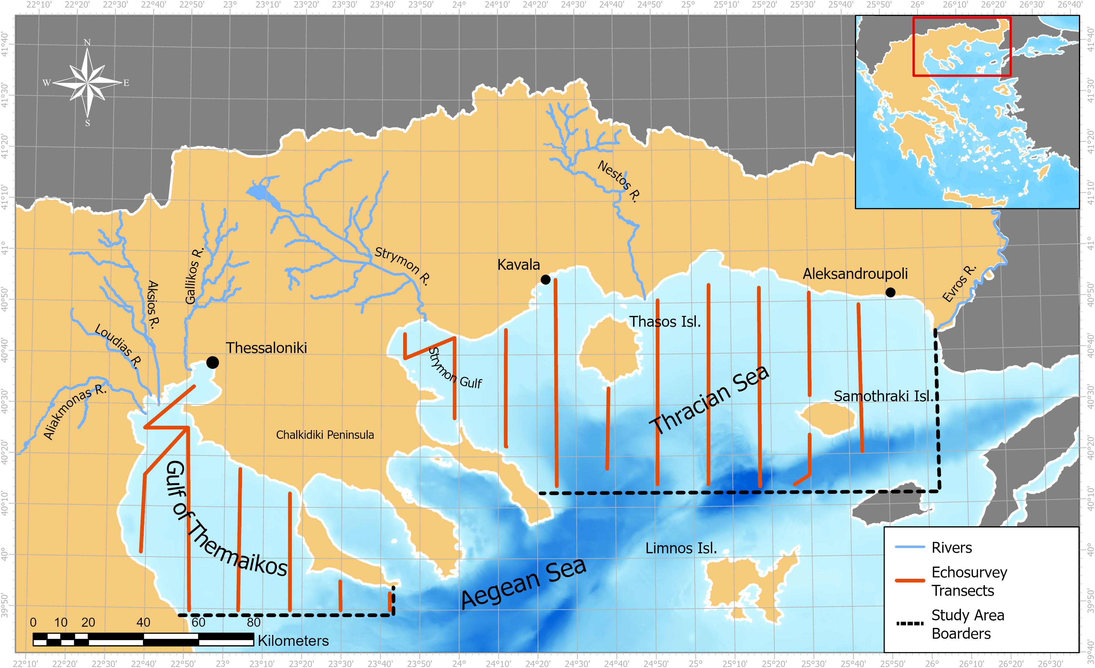
Figure 2 Map of the study area in the North Aegean Sea. The two examined sub-regions are the Gulf of Thermaikos in the West and the Thracian Sea in the East.
The North Aegean waters hold lower salinity levels compared to the South Aegean because of a) the inflow of Black Sea Water (BSW) masses through the Dardanelles strait at the eastern part of the TS (Somarakis et al., 2002) and b) the river outflows in the case of GT (Androulidakis et al., 2021). The BSW surface layer can provide salinity values as low as 36‰, whereas in the rest of the Aegean, salinity in the range of 39-40‰ is observed (Karageorgis et al., 2012). The Aegean is generally characterized as an oligotrophic sea, but the North Aegean typically has higher nutrient concentration than the South Aegean, concerning phosphates and silicates (Varkitzi et al., 2020). The nutrient decrease based on latitude is also translated to primary production values from 0.51 mg °C m-2 h-1 in the North Aegean to 0.22 mg °C m-2 h-1 in the South (Psarra et al., 2022). In coastal areas where river outflows are present, such as the GT, productivity is sustained by the nutrients in the sea through deltas. Studies have shown that variability in productivity in such areas coincides with variability in nutrient flux through rivers (Tsiaras et al., 2014).
The latitudinal decrease in primary productivity from North to South is also reflected in fisheries production. The great depths and trenches that are in between the continental shelves of the North Aegean and the Southern areas also act as barriers for the migration of small pelagic fish populations and as such they are confined to higher latitudes (Giannoulaki et al., 2005; Gkanasos et al., 2021). This is also reflected in Greek fisheries fleet distribution, where purse seine fishing is mainly conducted in the North Aegean in case of both number and size of vessels (Machias et al., 2008). Furthermore, the State of Mediterranean and Black Sea Fisheries 2022 report from FAO, 2022 includes three Greek ports in the top ten list of relative contributions to total landings in the Eastern Mediterranean sub-region, all of which are located in the North Aegean.
According to the same report though, the total captures of anchovy and sardine remain relatively steady in the last decade for Greek fisheries, whereas for the Mediterranean the sardine landings are declining. Tsikliras et al., 2015 highlighted the increased overexploitation status of the Eastern Mediterranean and future scenarios hint that the climate change will add additional pressures to small pelagic species (Gkanasos et al., 2021).
2.2 Data
The environmental proxies used as the independent variables for modelling the spatial distribution of anchovy and sardine were selected based on their ecological profile in the study area. In this section more specific information is provided regarding the ecological profile of anchovy and sardine in the area of interest. Furthermore, the in-situ data will be described along with satellite dataset chosen to extract from the environmental proxies.
The most crucial process that can be recorded and monitored by satellite data is the creation of the base of the food chain, expressed by chlorophyll concentration and primary productivity. Both target species are small pelagic feeders mainly targeting small particle prey (zooplankton), including copepods, nauplii, gastropods and decapod larvae (Nikolioudakis et al., 2014). There are available models that predict the spatial distribution of zooplankton concentration, but their spatial distribution does not suite the purpose of this methodology. Instead, this study lays on the fact that zooplankton preys on phytoplankton and thus the CHL concentration was chosen as a proxy for describing potential food fields (Siokou et al., 2014).
Another environmental parameter that can be quantified through satellite systems and plays a vital role in the behavior of pelagic fish is SST. SST monitoring can identify areas where upwelling occurs (Pisoni et al., 2014; Huang et al., 2021) and it is an important factor both for the spatial distribution of the species and for the preference of breeding areas (Takasuka et al., 2008). SST through remote sensing can be helpful in oceanic circulation mapping, a detrimental factor in pelagic fish spatial distribution monitoring. For example, the TS contains various productive fishing grounds due to its wide continental self and favorable oceanographic conditions, influenced by the BSW. A particular oceanographic formation with great ecological impact is the gyre of Samothraki, which can be observed at different locations seasonally (Zervakis and Georgopoulos, 2002). The Samothraki gyre acts as an entraining mechanism for mesozooplankton and larvae with high ecological value (Somarakis and Nikolioudakis, 2007). Due to high concentrations of food, anchovy tends to accumulate at the gyre’s periphery, while sardine on the other hand usually is not associated with the gyre and is found closer to shore (Tsoukali et al., 2019). Furthermore, Reese et al., 2011 showed that the distribution of anchovy and sardine populations around thermal fronts differs significantly from the random distribution and that species tend to be attracted to them.
Another notable Essential Oceanographic Variable (EOV) for spall pelagic fish spatial distribution modeling is salinity. Salinity is a detrimental factor for both target species, as low salinity areas such as the frontal areas created by river plumes, are highly associated with increased spawning activity (Morello and Arneri, 2009). But sea surface salinity is only provided through satellite derived models at a course resolution of 4km and is not suitable for the purpose of this study. Further implementations could try to incorporate downscaling techniques to include such information (Chatziantoniou et al., 2022).
It should be noted that this methodology treats the study area as a 2-dimensional space and does not reflect the full complexity of the marine ecosystem. For example, Sentinel-3’s OLCI and ocean color sensors in general calculate the CHL concentration at the penetration depth, which usually corresponds to the first few meters below the sea surface (Moutzouris-Sidiris and Topouzelis, 2021). Examples of 3D small pelagic fish spatial distribution modeling in the North Aegean are present in the bibliography, but their implementation require additional data in the form of survey transect measurements, oceanic circulation modeling and/or 3D satellite models (Tsoukali et al., 2019; Gkanasos et al., 2021). In the case of the first two, continuous monitoring will not be possible due to the high cost and analysis time and the latter option lacks the spatial resolution of the proposed methodology.
The in-situ data that were used to train the models were derived from a two-year acoustic survey aiming to assess the biomass of anchovy and sardine population in North Aegean Sea. The survey was conducted by the Hellenic Centre of Marine Research (HCMR) through the MEDIAS project within the EU DCF framework and each acoustic measurement corresponds to one square nautical mile (Giannoulaki et al., 2021; Leonori et al., 2021). The data refer to biomass measurements in tonnes for the summer months of 2016 (31/05/2016 to 27/06/2016) and 2019 (15/06/2019 to 21/07/2019). Each measurement was classified based on ‘Presence’ and ‘Absence’, whether it presented biomass greater than 0 tonnes. In total, in-situ measurements add to 937 observations for the TS and 405 for the GT. From the total amount of observations, anchovy biomass greater than zero was found in 292 cases (31.2%) in the TS and 132 (32.6%) in the GT dataset. On the other hand, Sardine is more imbalanced with only 62 (6.6%) observations with presence and 30 (7.4%), for TS and GT respectively.
Environmental proxies for modeling the spatial distribution anchovy and sardine were retrieved from the Sentinel-3 satellite mission. The spatial resolution of Sentinel-3 data ranges from 300m to 500m with a temporal coverage of 1-2 days. The proxy dataset includes chlorophyll-a concentration (CHL mg/m3), Sea Surface Temperature (SST °C), the gradients of both CHL and SST as proxies of oceanic fronts (CHL_GRAD mg/m3/500m and SST_GRAD °C/500m), and the distances from both ocean color and thermal fronts (OC_FR_DIST and THERMAL_FR_DIST).
SST data are acquired from the Sea and Land Sensor Temperature Radiometer (SLSTR) sensor with a spatial resolution of 500m over sea. CHL is retrieved from the Sentinel-3 onboard sensor Ocean and Land Color Instrument (OLCI) with the use of the C2RCC neural network (Brockmann et al., 2016). The OLCI sensor is designed to yield data with similar spectral characteristics to the MERIS sensor. Its primary purpose is to provide information related to ocean color and biological processes. It holds a total of 21 spectral bands and provides ocean-color biophysical parameters at a resolution of 300m. Due to the difference in spatial resolution with the SST dataset, both variables were collated in a common 500m grid.
Aside from the data retrieved from satellite sources, a bathymetry dataset, obtained from the European Marine Observation and Data Network (EMODnet) bathymetry portal, was also used for the model training. This final bathymetry dataset has a spatial resolution of 115m and is a combined product of both acoustic surveys with filled gaps from satellite altimeter measurements.
2.3 Pre-processing
In this paper, the methodology for ocean front extraction follows a modified gradient-based approach (Spondylidis et al., 2020). The gradient is calculated for CHL and SST with the scope to identify and map ocean color and thermal surface fronts, respectively. The gradients on the x and y axes of the images are extracted using the Sobel operator with a kernel size of 3×3 (Eq. 1 & 2). Finally, the gradient is calculated through the overall magnitude with the directional ones (Eq. 3).
Where Gx and Gy are the directional gradients of x-axis (horizontal) and y-axis (vertical) of the image respectively, Gn the gradient magnitude for date n and Imn the spatial dataset (either CHL or SST).
The results of Equation 3 after being applied to the CHL and SST datasets refer to the CHL_GRAD and SST_GRAD, respectively used to train the models. Even though these datasets do not directly represent oceanic fronts, they act as non-discrete proxies for various circulation phenomena. High-gradient areas could indicate areas where two different water masses meet and create an eddy or a front. After the gradient estimation for each parameter, strong magnitudes are separated from weak. This process is achieved with the use of a two-step adaptive threshold which is applied to remove both weak gradients and extremely strong ones that are caused by data noise. The retained areas are then thinned iteratively to produce one-pixel wide continuous lines.
Even though mesoscale oceanic fronts are correlated to pelagic fish populations, fish are often associated with the buffer zone around the front (Belkin, 2021). To incorporate this information in the models, new data are created that depict the distance in meters to the closest front. Again, this procedure is replicated twice, once for the thermal fronts (THERMAL_FR_DIST) and another for the ocean color fronts (OC_FR_DIST).
Data processing and modeling were performed in the R language with the mgcv (Logistic Regression and GAM models) and randomForest (Random Forest model) packages. Before the modeling phase, the dataset was divided into training and validation subsets at percentages of 70% and 30% respectively. The data separation was conducted to ensure unbiased accuracy metrics, as the validation dataset would not be used through the modeling phase.
2.4 Spatial distribution modeling
As a first step of the spatial distribution modeling, a brief explanatory descriptive analysis was conducted to showcase the relation of the echosurvey data to the environmental. The Pearson correlation was calculated and plotted to reveal potential bivariate collinearity between the independent variables. Then boxplots were drawn for the Presence/Absence occurrences against the distribution of each variable. The boxplots can reveal how well each independent variable could potentially be used to describe and separate the dataset.
The satellite environmental proxies and the bathymetric data were used to model the anchovy and sardine presence by fitting the in-situ acoustic biomass measurements. Three models were tested, a) Logistic Regression (Logit), which is a form of multivariate linear regression used when the dependent variable is discrete and has two values denoting ‘success’ and ‘failure’ or, in the case of this paper, ‘Presence’ and ‘Absence’. b) GAMs, which compute indefinite functions for the independent variables associated with the dependent variable through a link function. Because the independent variable is binary, the logit equation was chosen as the link function. And c) Random Forest, a machine learning Ensemble Classifier, whose individual classifiers consist of decision trees.
After the data preparation, the three classification models were applied for each area and each species. To maximize the models’ performance, a new detection threshold was assessed for each iteration, different from the default of 0.5 response. The threshold was calculated through an iterative process of model specificity and sensitivity maximization with the Youden’s index (Youden, 1950).
Various GAM models were designed and tested with different combinations of smooth functions. Because they were trained with binomial data, the logit link function was supplied in all iterations. The best-performing models were the ones that used a mixture of smooth functions—specifically, the spline smooth function for all the variables. Additionally, the interactions of SST and CHL with bathymetry were included with the tensor smooth function. Tensor smooth was the more appropriate smooth function as the variables have different measuring units at different scales (Wood, 2006). The smoothness parameters were calculated through the REML algorithm. The Random Forest values of ntree and mtry were set at 400 trees and 4 variables, respectively.
Model validation and assessment was performed based on several metrics, to outline the best performing model per species and area. Overall model accuracy was calculated through confusion matrices. Each matrix was created with direct comparison of the model results to the independent 30% validation dataset. The Receiver Operating Characteristic (ROC) curve and the Area Under Curve (AUC) were used to rank the models based on their ability to correctly classify each observation, compared to a random selection (Bradley, 1997). Furthermore, Taylor graphs were constructed to rank models based on the standard deviation, correlation, and the Root Mean Square Error (RMSE), compared to the validation dataset (Taylor, 2001). The best performing model for each case was decided based on “voting” by these 5 metrics.
Classification of Presence/Absence though cannot reveal the magnitude of potential abundance of the species in an area and in that regard another regression model is tested based on the RandomForest algorithm. The regression aims to see if quantification of the species’ “Presence” would be possible. This information would allow the distinction of the potential abundance between regions. For example, two areas could have the necessary environmental characteristics to host fish populations, but one could be more favorable and attract bigger numbers. Through biomass regression, this detail could be added to the results. In general, the classification aims to set the boundaries of potential fish distribution with easy-to-interpret maps and results, whereas the regression modeling can add more information but with probable noise.
The Random Forest regression models were validated with Leave One Out cross-validation method. Cross-validation was selected as the accuracy assessment method due to the small dataset. The statistical error indices used were the RMSE, the Mean Absolute Error (MAE), and the Mean Bias Error (MBE). MAE and MBE have the same units as the dependent variable, and they are a good indication of the model’s bias. The significance of the variables in the Random Forest model was evaluated using the accuracy reduction indices and the Gini Impurity. The Gini Impurity Index is an indicator that measures the importance of variables through their role in decision-making. Because both high values of accuracy reduction and Gini impurity indicate high variable importance, the variables that fall farther from the center of the plot axis are the more significant. The term accuracy reduction refers to whether the model’s accuracy will be reduced if the variable in question is subtracted. The value corresponds to the magnitude of the decrease on the scale of 1. Random Forest models in every new decision or branch (split) they create in any tree, try to maximize the reduction of the ‘Impurity’ added. Thus, a decision that significantly reduces Impurity is considered important, and the variable based on which this decision was made is also regarded as important (Nembrini et al., 2018).
After the selection of the best performing models, the methodology was applied on Sentinel-3 daily data for a scene in 22/07/2019. The maps are used to showcase the capabilities of the proposed methodology and compare it to existing efforts and findings. The resulting maps were produced at a spatial resolution of 500m.
3 Results
3.1 Descriptive analysis
In this section, the statistical interactions of the variables are explored in order to provide insight at the later modeling phase. Figure 3A showcases the correlation, between the anchovy and sardine biomass data from the TS and the remote sensing products. Anchovy biomass in the TS dataset does not present any strong correlation with any variable. Perhaps the strongest correlation lies with the bathymetry, which is positive at a scale of 0.4. Even though weak, the directions of the correlation between biomass and SST and CHL are negative and positive, respectively. Weak correlation magnitude between the dependent and independent variables can hint that if the models can accurately represent the biomass distribution, the reason lies in the interactions between the variables and not in individual ones. Sardine correlations are even weaker and do not exceed 0.2 magnitudes with any independent variable.
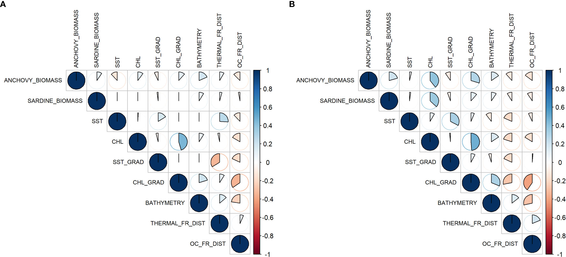
Figure 3 Correlation plot between anchovy and sardine biomass and the independent variables for (A) the TS dataset and (B) the GT dataset.
Data correlation for the GT dataset (Figure 3B) presents some essential differences that could hint at different interactions of the target species to their environment. The most obvious is the higher correlation of anchovy and sardine to chlorophyll-a levels. Furthermore, a negative correlation to the THERMAL_FR_DIST is showcased, which is the opposite of the respective in the TS dataset. Comparing the two species, they present similar characteristics except for anchovy, which shows a higher correlation to CHL_GRAD.
Strong correlations between the independent variables could indicate redundancy, and highly correlated pairs could be excluded. Such a pair is the CHL with its gradient where the correlation > 0.8. Because each represents a different aspect of the same parameter, one should be excluded from the modeling phase. Looking at the correlation of CHL with OC_FR_DIST, there is a negative correlation between the two but not a strong one. Considering that the peak gradient usually is present at lower distances to fronts, it could indicate that a potential selection of parameters would be CHL and OC_FR_DIST with the elimination of CHL_GRAD, as the distances could cover a portion of the information excluded without introducing strong collinearity within the models.
After the classification of the biomass to the Presence and Absence of the species, boxplots were drawn to identify proxies with potential valuable data separation capabilities (Figure 4). The CHL concentration was drawn on a logarithmically transformed to be more visible. For the TS, SST does not provide a clear distinction between the datasets, even though the fish presence tends to fall in areas with cooler waters for anchovy and sardine. On the other hand, CHL separates the Presence and Absence classes better, where higher concentrations of chlorophyll favor the presence of fish. The gradients of both SST and CHL present similar data separation characteristics to those of the original parameters. Focusing on the boxplot of the SST_GRAD, it is interesting that higher values of gradient magnitude do not favor the presence of the fish populations but moving on to the distance variables, it is showcased that the fish can more frequently be located at a distance around the 10km mark from the closest thermal front. On the contrary, fish tend to be closer to the ocean color fronts. Finally, the bathymetry seems to be a limiting factor for the fish distribution as the anchovy and sardine biomass is concentrated almost exclusively above the 200m isobath.
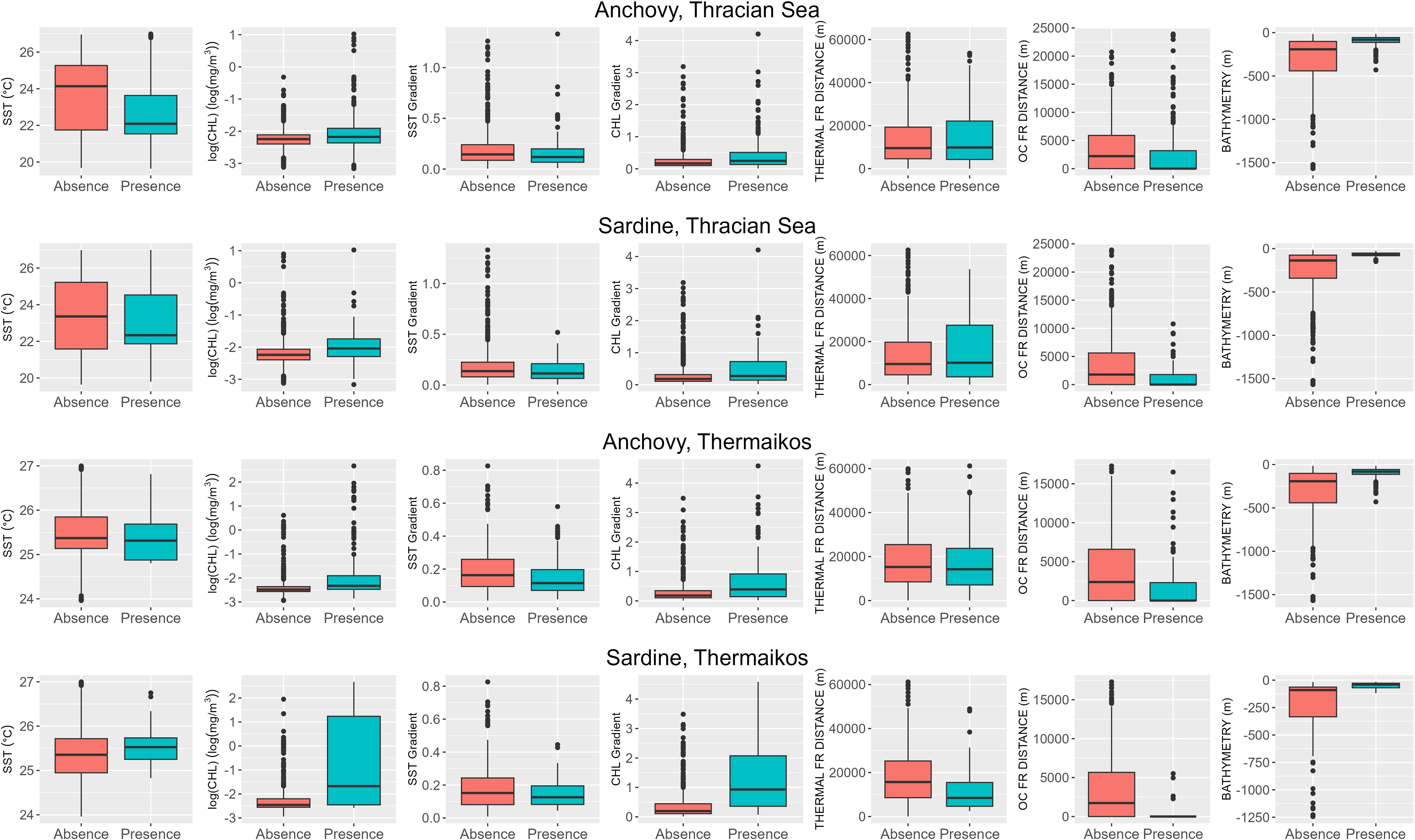
Figure 4 Boxplots between the classified in-situ measurements and all the independent variables for each species and each area. Orange is for ‘Absence’, and Green is for ‘Presence’.
Similarly, to observations made in the correlation analysis, there are differences between the GT dataset and the TS one. Also in this case, SST does not present a clear separation between the datasets. Anchovy biomass tends to concentrate in cooler waters, and sardine at more intermediate. CHL separates the data better, with sardine being in areas with higher concentrations. All other variables present similar patterns with the data of TS, apart from the distance to fronts for sardine. Sardine seems to be at closer distances to both types of fronts, and in the case of the ocean color ones, it is found in a proximity of 1km.
3.2 Classification models
Logistic regression was trained using all the variables except the CHL_GRAD. This variable presents relatively high collinearity with CHL concentration in both study areas and could artificially inflate the importance or weight. The logistic regression models for the TS presented moderate accuracy values, based on the confusion matrices (Supplementary Table 1), at the level of 73% and 68% for anchovy and sardine, respectively (Table 1). For the GT the models performed a little better for both species at 75% accuracy.
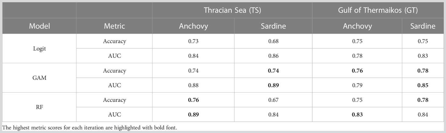
Table 1 Accuracy and AUC scores for each model of anchovy and sardine.
GAMs performed marginally better than the logistic regression in all instances. For anchovy in both TS and GT the improvement in accuracy was only by 1%. The biggest differences were for sardine in TS with 74% accuracy and for GT with 78% accuracy, which correspond to +6% and +3% respectively. To avoid potential collinearity issues, the variable CHL_GRAD was excluded from the GAMs for the same reasons explained in the logistic regression model section. The selected models are given in Supplementary Table 2 along with the partial effect plots in Supplementary Figures 1–4.
Random Forests on average performed similarly to the GAMs. They performed the best for anchovy in TS with 76%, and for sardine in GT with 78%. For sardine in TS Random Forests had an accuracy of 67% which was worse than both GAMs and the Logit models. Accuracy for anchovy in GT was similar to the other models at 75% which is only worse than the GAM iteration by 1%.
Based on the AUC metric, the Random Forest models performed better in the anchovy models, whereas GAMs performed the best in the sardine models (the ROC plots are also provided in Supplementary Figure 6). Contradictions are present though for the model of anchovy in GT, where the accuracy is higher for GAMs and the AUC is higher for Random Forest. Huang and Ling, 2005 have showcased that such contradictions in the accuracy and AUC metrics are possible. In their empirical trials they proved that AUC is a more consistent and discriminating model performance metric than accuracy.
To conclude on the best performing models an additional evaluation step was conducted through Taylor diagrams (Figure 5). Taylor diagrams compare each model based on three criteria, a) standard deviation of the predictions compared to the observed-validation data, b) correlation of the predictions and the observed-validation data, and c) the RMSE. Models whose predictions have the most similar standard deviation to the observed dataset, the highest correlation and the lowest RMSE are ranked higher than the others.
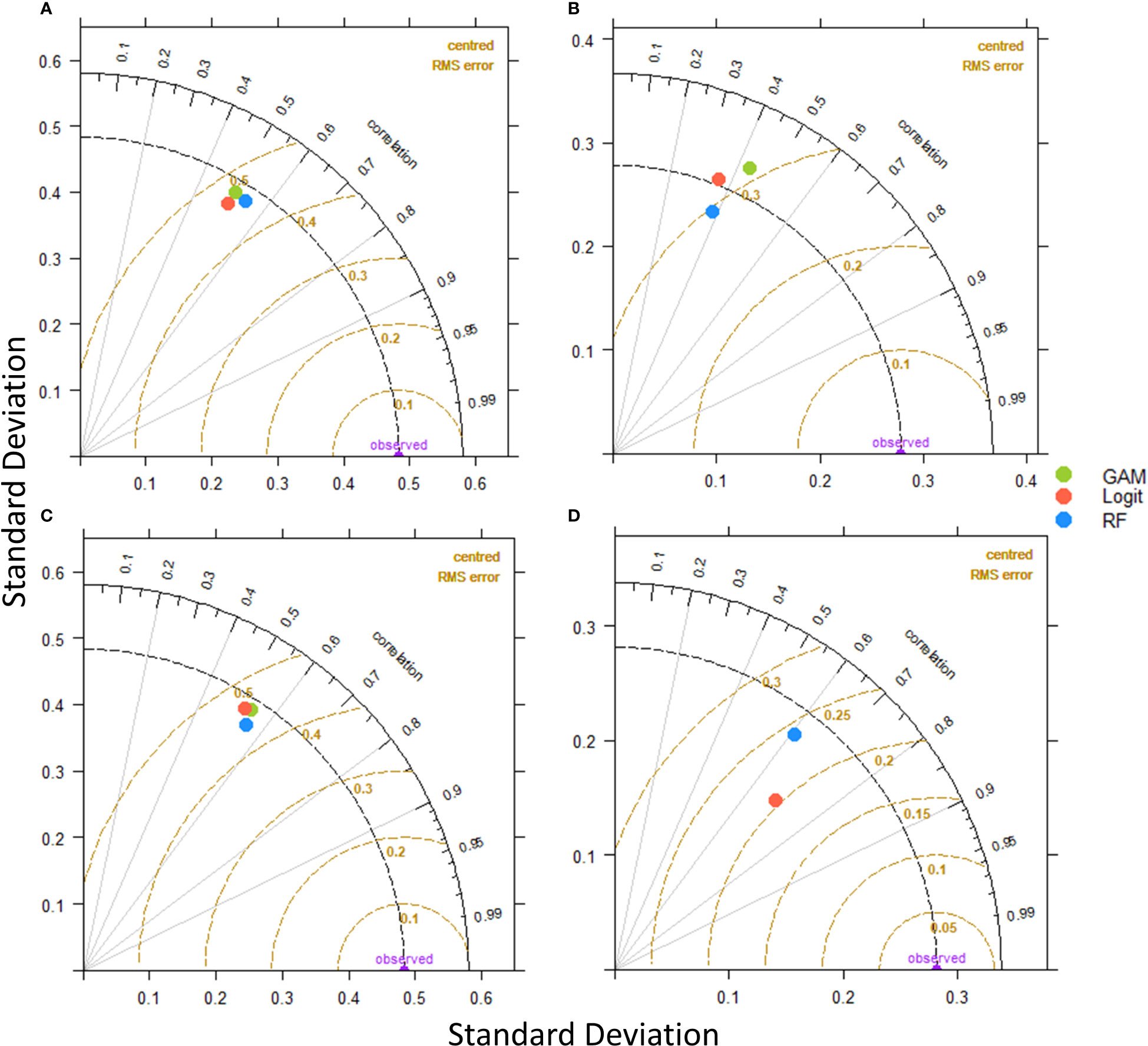
Figure 5 Taylor diagrams for Logistic regression, GAMs and Random Forest models comparison. (A) Anchovy in Thracian Sea, (B) Sardine in Thracian Sea, (C) Anchovy in Gulf of Thermaikos and (D) Sardine in Gulf of Thermaikos.
Through the Taylor diagrams for the anchovy models in TS, Random Forest is the best performing. Even though all the models’ metrics are close, Random Forest has the lowest RMSE score and highest correlation to the validation data. For sardine in TS the interpretation is more difficult, as no model distinguishes itself. Specifically, Logit has the most similar standard deviation to validation dataset, Random Forest has the lowest RMSE and GAM has the highest correlation. On the other hand, the Random Forest for anchovy in GT is better in both the RMSE and correlation metrics. Finally for sardine in GT, the Logit model scored the highest through the Taylor diagrams, as it presented both the lowest RMSE and the highest correlation.
The final decision of which model was the best for each occasion was taken by considering all 5 metrices through voting. Random Forest was the best model for anchovy in TS (4 out of 5) and anchovy in GT (3 out of 5). For sardine in TS and GT the GAMs where selected as the best performing as they had the best score in 3 out of 5 metrics in both cases.
3.3 Random Forest regression
Accuracy assessment of the regression models is performed with a 99 iteration Leave-One-Out cross-validation (Table 2). Similarly, to the classification models, the anchovy biomass model for the TS presents the best scores with the mean variance explained by the model at a scale of 86. Small values of the MBE and MAE across all models indicate low overall bias, considering that they differ in two orders of magnitude with the maximum in-situ biomass. The best RMSE score is also present in the anchovy model of the TS at a scale of 2.67 and a variation of 21. RMSE variation for the other three models is higher, indicating that the accuracy assessment could be hindered due to the dataset imbalance. Additionally, scatter plots of predicted against observed values are provided in Supplementary Figure 5 for each regression model.
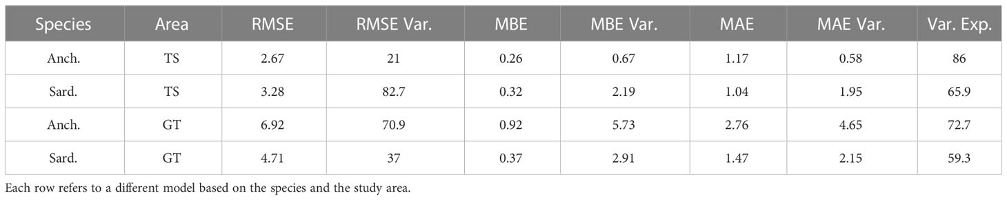
Table 2 Accuracy indices of RMSE, MBE, and MAE through Leave-One-Out cross-validation.
Concerning the importance of each independent variable for the anchovy models, SST and bathymetry were identified as two of the most significant ones in both the TS and the GT (Figure 6). Especially, in the case of the TS model, by excluding the SST or the bathymetry would increase the MSE by at least 55 tonnes, whereas the other variables would only increase by a maximum of 32 tonnes (Figure 6A). In the GT, though, the most important variables, even more than SST and bathymetry, are CHL and CHL_GRAD (Figure 6C). These four have the highest node purity score, as well as their exclusion, would increase the MSE by more than 120 tonnes. This difference could be attributed to the fact that CHL has a stronger correlation with fish biomass in the GT than the TS, as observed through the correlation plots.
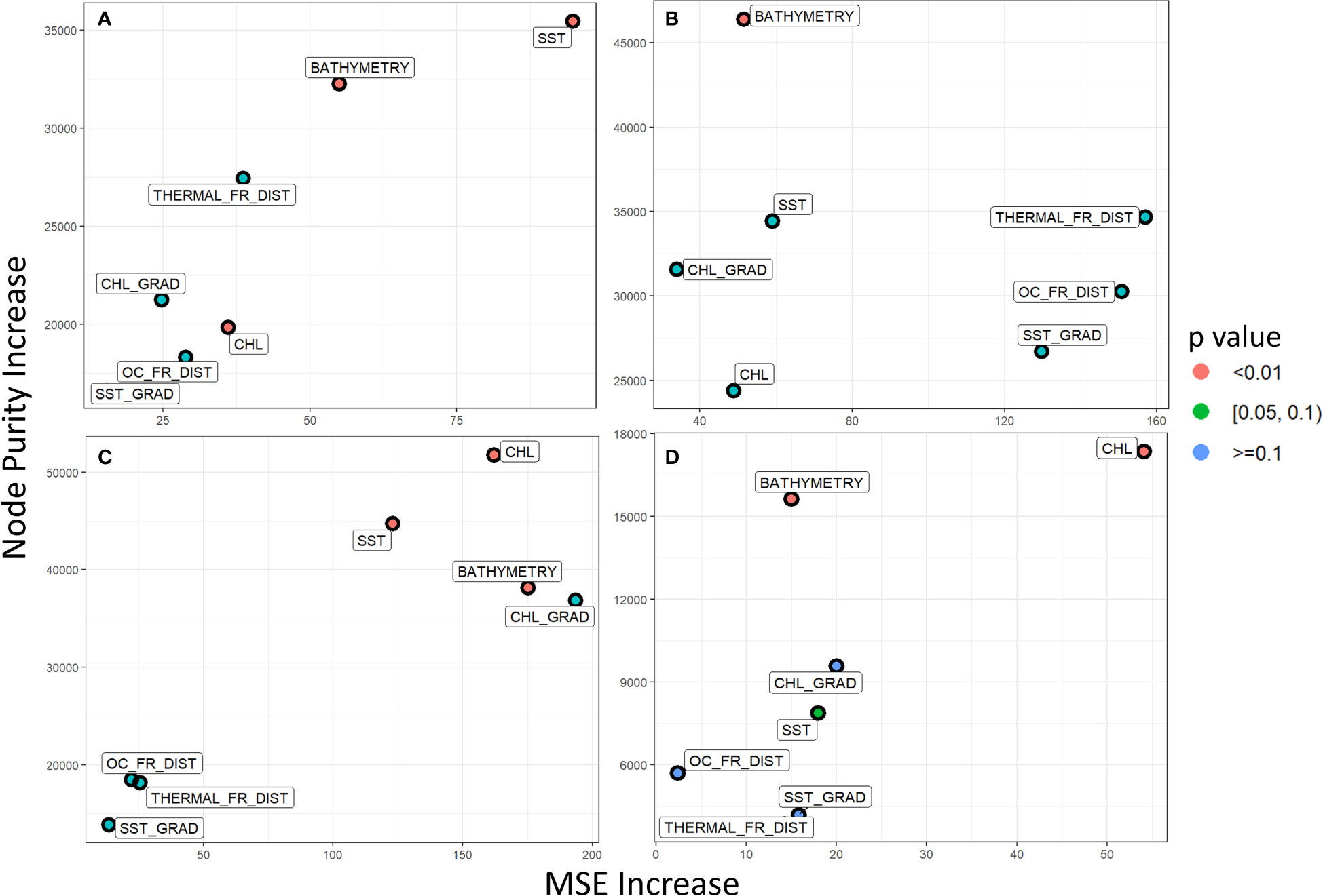
Figure 6 Multi-way variable importance plot for the Random Forest Regression Models for each species and each area. (A) Anchovy in TS, (B) Sardine in TS, (C) Anchovy in GT and (D) Sardine in GT. The p-value refers to the significance of each variable if it is used for splitting more often than would be the case if the selection was random.
The sardine biomass regression model showcases again bathymetry as one of the most important variables, as in both areas it presents some of the highest scores node purity increase (Figures 6B, D). The other important variables differ depending on the region. For example, for TS both THERMAL_FR_DIST and OC_FR_DIST have the highest potential impact on MSE increase if they were to be excluded from the analysis. On the other hand, similarly to what was observed for the anchovy models, CHL is the most important variable in the GT model. Bathymetry generally showcases high node purity in all models as it is an apparent spatial separation factor for fish abundance, where no fish are observed at areas with depths >200m.
4 Discussion
In the present study, the accuracy of the results, in terms of % success in the identification of potential Presence/Absence occurrences, for anchovy ranged between 73% to 76%, and for sardine 67% to 78%, proving that higher resolution data can be used for small pelagic fish distribution mapping in smaller and more complex geographical regions. These results find the described methodology in accordance with recent studies and modeling techniques. Nurdin et al., 2017 constructed GAMs with independent variables SST and CHL at 4 km resolution to identify mackerel fishing zones on the coast of Indonesia. By comparing their results with real Catch Per Unit Effort (CPUE) fishing data, they estimated that the accuracy of their predictions exceeds 83%. Machine learning techniques and specific artificial neural networks have been used for similar purposes. In the study by Wang et al., 2015 researchers constructed a neural network that takes as input SST, Sea Surface Height (SSη), and chlorophyll-a, and which predicts the existence of potential fishing zones with 80% success (a similar application was developed by Nuno et al., 2005).
Aside from bathymetry, CHL was one of the most important environmental proxies to sardine biomass modeling in both study areas. In TS the distance to ocean color fronts and in GT the CHL concentration by itself. The CHL dependency could be indicative to sardine’s preferred seasonal feeding mechanism. Sardines are omnivorous feeders, and they can switch between particle-feeding, for mesozooplankton, and filter-feeding, for phytoplankton, depending on the availability and abundance of prey per season (Bode et al., 2004; Cunha et al., 2005). In winter, when larger zooplankton species (copepods) are abundant they use the particle-feeding technique to catch their prey (Somarakis et al., 2006). On the other hand, in the summer it has been observed that sardines switch to filter-feeding to prey on picoplankton and smaller size zooplankton, because it is more energy efficient (Nikolioudakis et al., 2012). In contrast to sardines, anchovies are feeding purely on microzooplankton and mesozooplankton for their energy intake (Catalán et al., 2010).
Anchovy in TS was highly dependent on bathymetry, SST and the distance to thermal fronts. There is correlation between phytoplankton and zooplankton abundance but with a temporal lag of 1-1.5 months (Frangoulis et al., 2017), so no direct link to CHL concentration is expected. Instead, potential adult anchovy habitats have been correlated to bottom depth and sea level anomaly (Giannoulaki et al., 2013) because they are linked to zooplankton aggregations. Furthermore, the significance of depth and temperature could be related to spawning, which for anchovy typically occurs between late spring to early summer in the Mediterranean and the Aegean (Tsoukali et al., 2019; Basilone et al., 2020).
In the work of Schismenou et al., 2008, anchovy and sardine egg samples were analyzed for the summer periods of 2003-2006, and the interaction of CHL with bathymetry were the key environmental proxies for spawning habitat characterization for both species, which does match the variable significance results for the GT but not the TS in the present study. In GT both species presented high affinity towards CHL concentration that indicates preference to highly productive areas. On the other hand, the GT is characterized by major river outflows which supply the gulf with waters containing high concentrations of suspended matter. In turbid waters, the C2RCC algorithm can overestimate CHL concentration resulting to misinterpretations (Vanhellemont and Ruddick, 2021). It could be hypothesized though, that if high CHL concentrations are attributed to turbulent river outflows, then that could link anchovy and sardine presence, in the GT, to low salinity areas, which is a known favorable environmental parameter for both species (Bonanno et al., 2016; Fernández-Corredor et al., 2021). Unfortunately, there are no available satellite products at the mandatory spatial resolution to test this hypothesis.
To showcase the application of the results on a spatial dataset, the best performing classification models, and the regression random forest models are applied to Sentinel-3 data for the date of 22/07/2019 (Figure 7). In this dataset, SST ranges from 24.35 – 30.22 °C (Figure 7A), and CHL concentration is across the area low at 0.15 mg/m3 (Figure 7B), with a peak at the Eastern side where the Evros estuary is located. On the model results, the isobaths of -200, -400, -700, and -1200m are drawn. The classification models of anchovy and sardine (Figures 7E, F respectively) showed fish aggregations at different locations per species in the study area. The anchovy model shows more occurrences of “Presence” locations in the NW region of Samothraki, the Gulf of Strymonikos and around Thasos island, whereas sardine is present more frequently at coastal areas.
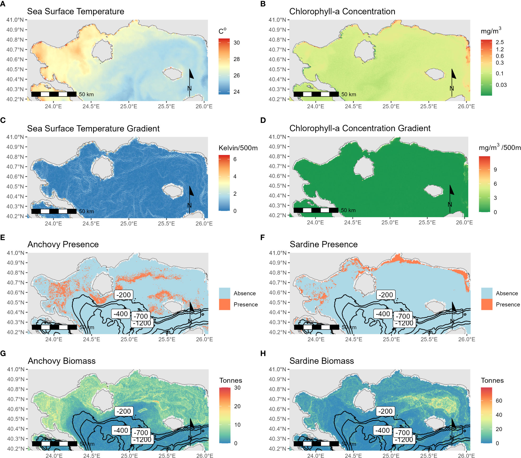
Figure 7 Maps for 22/07/2019 showcasing the results of both Random Forest classification and regression for the Thracian Sea. From left to right and top to bottom, (A) SST, (B) CHL concentration, (C) SST Gradient, (D) CHL concentration Gradient, (E) Anchovy presence classification results, (F) Sardine presence classification results, (G) Anchovy biomass regression results and (H) Sardine biomass regression results. Overlayed to the model result maps, the isobaths of -200m, -400m, -700m and -1200m are drawn.
Applying the Random Forest regression model on the dataset for anchovy presents intermediate biomass predictions across the study area around the 10 tonnes mark (Figure 7G). Some peaks are present NW of Samothraki Island and the Gulf of Kavala and Strymonikos. Anchovy high biomass predictions are observed at the same longitude as sardine but more offshore. These patterns were observed by Barra et al., 2015 based on samplings from 2004-2006 and 2008, which was attributed to interspecific competition alleviation. Similar conclusions were also discussed in the present study based on the difference of significance of each environmental proxy for the species’ spatial distribution modeling.
Sardine high biomass concentrations are observed NW, and N of Samothraki, with depths at a maximum of 80m (Figure 7H). The spatial distribution presented in this work matches the species’ profile as sardines showcase a general affinity to coastal areas, both in the winter, when they spawn at a maximum depth of 65m, and the summer months (Tugores et al., 2011). Giannoulaki et al., 2011 also observed that the seasonal migration of sardines is limited to coastal areas, and it does not exceed the 100m isobath. The depth restriction to sardine’s spatial distribution (Giannoulaki et al., 2005; Bellido et al., 2008; Giannoulaki et al., 2013) could explain why the bathymetry was the most significant variable in the Random Forest biomass model.
Evidently, the classification and the regression results provided significant differences. Especially for sardine the “Presence” areas do not match the high biomass concentration areas except for Strymonikos Gulf. This problem arises from the training dataset which is greatly imbalanced and hints that one model (classification or regression) may be underperforming. The dominance of “Absence” observations in the original dataset could cause the underprediction of “Presence” occurrences. Through the confusion matrices for GAM sardine model (Supplementary Material) only 14/26 “Presence” observations were correctly classified, meaning that the model has learned better to identify areas with no fish occurrences than areas with occurrences. To mitigate such an effect, the dataset could be balanced in such a way that “Presence” and “Absence” observations would be represented equally at 1:1 ratio. However, this would result in a small training dataset with just 124 observations for sardine in TS and 60 in GT, even before splitting to training and validation. The use of such a small dataset could result in biased overfitted results (Vabalas et al., 2019) and it was avoided. The distinction between the two methodologies could be investigated further with the use of additional larger and better represented datasets.
In the context of fisheries management, the spatial and temporal resolution of the results could cover various monitoring needs and shortcomings of the current state. Bellido et al., 2020 suggests that an effective fishery management framework should more regionalized, supported by the appropriate monitoring infrastructure. Higher resolution ocean color satellite observations are capable to support such a framework with continuous monitoring fish stock spatial distribution. At 500m resolution spatial differences in neighboring areas will be distinguishable and the authorities will be able to coordinate the fleet for maximum yield and minimum expenses and with the addition of being compliant with finer resolution fishing activity mapping (Janßen et al., 2018). Furthermore, the daily coverage in combination with Vessel Monitoring Systems (VMS) will allow continuous monitoring of the fleet and draw statistics on fishing effort in relation to potential fish abundance.
5 Conclusion
The present work explores the use of high spatial resolution data to map the spatial distribution of anchovy and sardine populations in smaller-scale areas. 12 classification models were tested, along with 4 regression models. Comparison with in-situ biomass acoustic measurements provides a strong case that similar methodologies can be used for general application in more regions. The classification techniques used in the study involved three types of models, logistic regression, GAMs, and Random Forest. High detection rates from all models were achieved. Furthermore, the biomass Random Forest regression produced minor bias errors with an acceptable fit to the dataset.
In the biomass regression models, each species presented different variable importance for each study area. Anchovy in the TS for example was more dependent on bathymetry, SST distribution, and distance to thermal fronts, compared to the GT results where CHL, SST, and bathymetry had a higher impact. The variable importance could indicate that fish aggregation in each region could depend on its specific environmental characteristics (i.e. the presence of river outflows). In any case, the main conclusion based on the divergent results is that regional models could be the best tactic in fish spatial distribution monitoring with the use of higher, than traditional, spatial resolution data.
The application of the models on spatial datasets revealed that many known areas with high aggregation of small pelagic fish populations were successfully detected. These areas are Samothraki Island and the Gulf of Kavala. No areas were detected below the 200m isobaths, which agrees with other scientific findings in the Mediterranean Sea mentioned in the discussion section. These observations, along with the models’ validation, hint that the methodology can be used to describe the preferred spatial distribution of the target species in fine resolution with high accuracy.
Incorporating higher spatial resolution data along with front detection allowed the inclusion of oceanographic features detrimental to small pelagic fish spatial distribution. This was proven from the results as the CHL gradient and the distance from thermal fronts were, in many cases, two of the most impactful variables in the regression models. Higher-resolution satellite data can detect smaller mesoscale features necessary for applications in small areas with complex geographies, like the Aegean Sea. The circulation in those areas produces highly biologically impactful fronts and gyres that generally could not be mapped with lower spatial resolution data.
The main limitation of the proposed methodology lies in its dimensionality. Satellite observations mainly capture the surface oceanographic conditions, thus limiting the available ecologically important information. The use of 3D models could provide insight at various depths with the additional benefit of other significant oceanographic parameters for marine spatial distribution modeling, like salinity levels and zooplankton concentration. Compared to satellite data, it is a tradeoff between data quantity and resolution.
Data availability statement
The original contributions presented in the study are included in the article/Supplementary Material. Further inquiries can be directed to the corresponding authors.
Author contributions
SS, MG, and KT contributed to conception and design of the study. SS performed the statistical analysis, modeling, and validation. MG and AM provided the field acoustic biomass data. SS wrote the article. MG and KT contributed critically to the revision. All authors contributed to the article and approved the submitted version.
Funding
This research has been co‐financed by the European Regional Development Fund of the European Union and Greek national funds through the Operational Program Competitiveness, Entrepreneurship, and Innovation, under the call RESEARCH – CREATE – INNOVATE (project code: T2EDK-02687).
Conflict of interest
The authors declare that the research was conducted in the absence of any commercial or financial relationships that could be construed as a potential conflict of interest.
Publisher’s note
All claims expressed in this article are solely those of the authors and do not necessarily represent those of their affiliated organizations, or those of the publisher, the editors and the reviewers. Any product that may be evaluated in this article, or claim that may be made by its manufacturer, is not guaranteed or endorsed by the publisher.
Supplementary material
The Supplementary Material for this article can be found online at: https://www.frontiersin.org/articles/10.3389/fmars.2023.1117704/full#supplementary-material
Supplementary Table 1 | Confusion Matrices for each classification model. The first sheet corresponds to the logistic regression results, the second to the GAMs results, and the third to the Random Forest results.
Supplementary Table 2 | The selected GAM models’ formulas along with their respective deviance explained percentage.
Supplementary Data Sheet 1 | Abbreviation table of all the acronyms used in the paper.
Supplementary Figure 1 | The partial effects of the independent variables for the anchovy in TS GAMs. The shaded orange areas represent the 95% confidence interval.
Supplementary Figure 2 | The partial effects of the independent variables for the sardine in TS GAMs. The shaded orange areas represent the 95% confidence interval.
Supplementary Figure 3 | The partial effects of the independent variables for the anchovy in GT GAMs. The shaded orange areas represent the 95% confidence interval.
Supplementary Figure 4 | The partial effects of the independent variables for the sardine in GT GAMs. The shaded orange areas represent the 95% confidence interval.
Supplementary Figure 5 | Scatterplots of the predicted vs observed biomass values in tonnes retrieved from the Random Forest regression models. (A) Anchovy in TS, (B) Sardine in TS, (C) Anchovy in GT, (D) Sardine in GT. The black line represents the 1:1 line.
Supplementary Figure 6 | The ROC plots for the classification models. They are divided by species and by region.
References
Androulidakis Y., Kolovoyiannis V., Makris C., Krestenitis Y., Baltikas V., Stefanidou N., et al. (2021). Effects of ocean circulation on the eutrophication of a Mediterranean gulf with river inlets: The northern thermaikos gulf. Cont. Shelf Res. 221, 104416. doi: 10.1016/j.csr.2021.104416
Apostolopoulos D., Nikolakopoulos K. (2021). A review and meta-analysis of remote sensing data, GIS methods, materials and indices used for monitoring the coastline evolution over the last twenty years. Eur. J. Remote Sens. 54, 240–265. doi: 10.1080/22797254.2021.1904293
Arur A., Krishnan P., George G., Goutham Bharathi M. P., Kaliyamoorthy M., Hareef Baba Shaeb K., et al. (2014). The influence of mesoscale eddies on a commercial fishery in the coastal waters of the Andaman and nicobar islands, India. Int. J. Remote Sens 35, 6418–6443. doi: 10.1080/01431161.2014.958246
Barra M., Petitgas P., Bonanno A., Somarakis S., Woillez M., Machias A., et al. (2015). Interannual changes in biomass affect the spatial aggregations of anchovy and sardine as evidenced by geostatistical and spatial indicators. PloS One 10, e0135808. doi: 10.1371/journal.pone.0135808
Basilone G., Ferreri R., Barra M., Bonanno A., Pulizzi M., Gargano A., et al. (2020). Spawning ecology of the European anchovy (Engraulis encrasicolus) in the strait of Sicily: Linking variations of zooplankton prey, fish density, growth, and reproduction in an upwelling system. Prog. Oceanogr. 184, 102330. doi: 10.1016/j.pocean.2020.102330
Baudron A. R., Brunel T., Blanchet M. A., Hidalgo M., Chust G., Brown E. J., et al. (2020). Changing fish distributions challenge the effective management of European fisheries. Ecography 43, 494–505. doi: 10.1111/ecog.04864
Belkin I. M. (2021). Review remote sensing of ocean fronts in marine ecology and fisheries. Remote Sens. (Basel) 13, 1–22. doi: 10.3390/rs13050883
Bellido J. M., Brown A. M., Valavanis V. D., Giráldez A., Pierce G. J., Iglesias M., et al. (2008). Identifying essential fish habitat for small pelagic species in Spanish Mediterranean waters. in. Hydrobiologia, 171–184. doi: 10.1007/s10750-008-9481-2
Bellido J. M., Sumaila U. R., Sánchez-Lizaso J. L., Palomares M. L., Pauly D. (2020). Input versus output controls as instruments for fisheries management with a focus on Mediterranean fisheries. Mar. Policy 118, 103786. doi: 10.1016/j.marpol.2019.103786
Bode A., Teresa Álvarez-Ossorio M., Carrera P., Lorenzo J. (2004). Reconstruction of trophic pathways between plankton and the north Iberian sardine (Sardina pilchardus) using stable isotopes. Sci. Mar. 68, 165–178. doi: 10.3989/scimar.2004.68n1165
Bonanno A., Barra M., Basilone G., Genovese S., Rumolo P., Goncharov S., et al. (2016). Environmental processes driving anchovy and sardine distribution in a highly variable environment: the role of the coastal structure and riverine input. Fish Oceanogr. 25, 471–490. doi: 10.1111/fog.12166
Bonanno A., Giannoulaki M., Barra M., Basilone G., Machias A., Genovese S., et al. (2014). Habitat selection response of small pelagic fish in different environments. two examples from the oligotrophic Mediterranean Sea. PloS One 9, e101498. doi: 10.1371/journal.pone.0101498
Bradley A. E. (1997). The use of the area under the ROC curve in the evaluation of machine learning algorithms. Pattern Recognit. 30, 1145–1159. doi: 10.1016/S0031-3203(96)00142-2
Brekke C., Solberg A. H. S. (2005). Oil spill detection by satellite remote sensing. Remote Sens. Environ. 95, 1–13. doi: 10.1016/j.rse.2004.11.015
Brockmann C., Doerffer R., Peters M., Stelzer K., Embacher S., Ruescas A. (2016). Evolution of the C2RCC Neural Network for Sentinel 2 and 3 for the Retrieval of Ocean Colour Products in Normal and Extreme Optically Complex Waters. in ESASP, 54. Available at: https://ui.adsabs.harvard.edu/abs/2016ESASP.740E..54B/abstract.
Catalán I. A., Folkvord A., Palomera I., Quílez-Badía G., Kallianoti F., Tselepides A., et al. (2010). Growth and feeding patterns of European anchovy (Engraulis encrasicolus) early life stages in the Aegean Sea (NE Mediterranean). Estuar. Coast. Shelf Sci. 86, 299–312. doi: 10.1016/j.ecss.2009.11.033
Chatziantoniou A., Charalampis Spondylidis S., Stavrakidis-Zachou O., Papandroulakis N., Topouzelis K. (2022). Dissolved oxygen estimation in aquaculture sites using remote sensing and machine learning. Remote Sens. Appl. 28, 100865. doi: 10.1016/j.rsase.2022.100865
Colloca F., Garofalo G., Bitetto I., Facchini M. T., Grati F., Martiradonna A., et al. (2015). The seascape of demersal fish nursery areas in the north Mediterranean Sea, a first step towards the implementation of spatial planning for trawl fisheries. PloS One 10, e0119590. doi: 10.1371/journal.pone.0119590
Cunha M. E., Garrido S., Pissarra J. (2005). The use of stomach fullness and colour indices to assess sardina pilchardus feeding. J. Mar. Biol. Assoc. United Kingdom 85, 425–431. doi: 10.1017/S0025315405011367h
FAO (2022). “The State of Mediterranean and Black Sea Fisheries 2022. Rome: General Fisheries Commission for the Mediterranean. doi: 10.4060/cc3370en
Fauziyah, Setiawan A., Agustriani F., Rozirwan, Melki, Nurjuliasti Ningsih E., et al. (2022). Distribution pattern of potential fishing zones in the bangka strait waters: An application of the remote sensing technique. Egyptian J. Remote Sens. Space Sci. 25, 257–265. doi: 10.1016/j.ejrs.2021.12.003
Fernández-Corredor E., Albo-Puigserver M., Pennino M. G., Bellido J. M., Coll M. (2021). Influence of environmental factors on different life stages of European anchovy (Engraulis encrasicolus) and European sardine (Sardina pilchardus) from the Mediterranean Sea: A literature review. Reg. Stud. Mar. Sci. 41, 101606. doi: 10.1016/j.rsma.2020.101606
Frangoulis C., Grigoratou M., Zoulias T., Hannides C. C. S., Pantazi M., Psarra S., et al. (2017). Expanding zooplankton standing stock estimation from meso- to metazooplankton: A case study in the n. Aegean Sea (Mediterranean Sea). Cont. Shelf Res. 149, 151–161. doi: 10.1016/j.csr.2016.10.004
Giannoulaki M., Iglesias M., Tugores M. P., Bonanno A., Patti B., de Felice A., et al. (2013). Characterizing the potential habitat of European anchovy engraulis encrasicolus in the Mediterranean Sea, at different life stages. Fish Oceanogr. 22, 69–89. doi: 10.1111/fog.12005
Giannoulaki M., Machias A., Somarakis S., Tsimenides N. (2005). The spatial distribution of anchovy and sardine in the northern Aegean Sea in relation to hydrographic regimes. Belg. J. Zool. 135, 151–156.
Giannoulaki M., Pyrounaki M. M., Liorzou B., Leonori I., Valavanis V. D., Tsagarakis K., et al. (2011). Habitat suitability modelling for sardine juveniles (Sardina pilchardus) in the Mediterranean Sea. Fish Oceanogr. 20, 367–382. doi: 10.1111/j.1365-2419.2011.00590.x
Giannoulaki M., Valavanis V. D., Palialexis A., Tsagarakis K., Machias A., Somarakis S., et al. (2008). “Modelling the presence of anchovy engraulis encrasicolus in the Aegean Sea during early summer, based on satellite environmental data,” in Hydrobiologia (Netherlands: Springer), 225–240. doi: 10.1007/s10750-008-9498-6
Giannoulaki M., Zwolinski J., Gucu A. C., de Felice A., Somarakis S. (2021). The “MEDiterranean international acoustic survey”: An introduction. Mediterr. Mar. Sci. 22, 747–750. doi: 10.12681/mms.29068
Gkanasos A., Schismenou E., Tsiaras K., Somarakis S., Giannoulaki M., Sofianos S., et al. (2021). A three dimensional, full life cycle, anchovy and sardine model for the north Aegean Sea (Eastern mediterranean): Validation, sensitivity and climatic scenario simulations. Mediterr. Mar. Sci. 22, 653–668. doi: 10.12681/mms.27407
Godø O. R., Samuelsen A., Macaulay G. J., Patel R., Hjøllo S. S., Horne J., et al. (2012). Mesoscale eddies are oases for higher trophic marine life. PloS One 7, 1–9. doi: 10.1371/journal.pone.0030161
Hu C. (2021). Remote detection of marine debris using satellite observations in the visible and near infrared spectral range: Challenges and potentials. Remote Sens. Environ. 259, 112414. doi: 10.1016/j.rse.2021.112414
Huang Z., Hu J., Shi W. (2021). Mapping the coastal upwelling east of taiwan using geostationary satellite data. Remote Sens. (Basel) 13, 1–20. doi: 10.3390/rs13020170
Huang J., Ling C. X. (2005). Using AUC and accuracy in evaluating learning algorithms. IEEE Trans. Knowledge Data Eng. 17, 299–310. doi: 10.1109/TKDE.2005.50
Janßen H., Bastardie F., Eero M., Hamon K. G., Hinrichsen H. H., Marchal P., et al. (2018). Integration of fisheries into marine spatial planning: Quo vadis? Estuar. Coast. Shelf Sci. 201, 105–113. doi: 10.1016/j.ecss.2017.01.003
Karageorgis A. P., Georgopoulos D., Kanellopoulos T. D., Mikkelsen O. A., Pagou K., Kontoyiannis H., et al. (2012). Spatial and seasonal variability of particulate matter optical and size properties in the Eastern Mediterranean Sea. J. Mar. Syst., 105–108. doi: 10.1016/j.jmarsys.2012.07.003. 123–134.
Kürten B., Zarokanellos N. D., Devassy R. P., El-Sherbiny M. M., Struck U., Capone D. G., et al. (2019). Seasonal modulation of mesoscale processes alters nutrient availability and plankton communities in the red Sea. Prog. Oceanogr. 173, 238–255. doi: 10.1016/j.pocean.2019.02.007
Leonori I., Tičina V., Giannoulaki M., Hattab T., Iglesias M., Bonanno A., et al. (2021). History of hydroacoustic surveys of small pelagic fish species in the European Mediterranean Sea. Mediterr. Mar. Sci. 22, 751–768. doi: 10.12681/mms.26001
Lykousis V., Roussakis G., Alexandri M., Pavlakis P., Papoulia I. (2002). Sliding and regional slope stability in active margins: North Aegean trough (Mediterranean). Mar. Geol. 186, 281–298. doi: 10.1016/S0025-3227(02)00269-4
Machias A., Stergiou K. I., Somarakis S., Karpouzi V. S., Kapantagakis A. (2008). Trends in trawl and purse seine catch rates in the north-eastern Mediterranean. Mediterr. Mar. Sci. 9, 49–66. doi: 10.12681/mms.143
Mansor S., Tan C. K., Ibrahim H. M., Shariff A. R. M. (2001). “Satellite fish forecasting in south China sea,” in 22nd Asian Conference on Remote Sensing, (Singapore: Center for Remote Imaging, Sensing and Processing, National University of Singapore), 5–9. doi: 10.4238/2012.July.19.6
Mazor T., Possingham H. P., Edelist D., Brokovich E., Kark S. (2014). The crowded sea: Incorporating multiple marine activities in conservation plans can significantly alter spatial priorities. PloS One 9, e104489. doi: 10.1371/journal.pone.0104489
Miller P. I., Xu W., Carruthers M. (2015). Seasonal shelf-sea front mapping using satellite ocean colour and temperature to support development of a marine protected area network. Deep Sea Res. 2 Top. Stud. Oceanogr. 119, 3–19. doi: 10.1016/j.dsr2.2014.05.013
Morello E. B., Arneri E. (2009). Anchovy and sardine in the adriatic sea-an ecological review. Oceanogr. Mar. Biol. 47, 209–256. doi: 10.1201/9781420094220.CH5
Moutzouris-Sidiris I., Topouzelis K. (2021). Assessment of chlorophyll-a concentration from sentinel-3 satellite images at the Mediterranean Sea using CMEMS open source in situ data. Open Geosci. 13, 85–97. doi: 10.1515/geo-2020-0204
Nair P. G., Pillai V. N. (2012). Satellite based potential fishing zone (PFZ) advisories-acceptance levels and benefits derived by the user community along the kerala coast. Indian J. Fish. 59, 69–74.
Nembrini S., König I. R., Wright M. N. (2018). The revival of the gini importance? Bioinformatics 34, 3711–3718. doi: 10.1093/bioinformatics/bty373
Nikolioudakis N., Isari S., Pitta P., Somarakis S. (2012). Diet of sardine sardina pilchardus: An “end-to-end” field study. Mar. Ecol. Prog. Ser. 453, 173–188. doi: 10.3354/meps09656
Nikolioudakis N., Isari S., Somarakis S. (2014). Trophodynamics of anchovy in a non-upwelling system: Direct comparison with sardine. Mar. Ecol. Prog. Ser. 500, 215–229. doi: 10.3354/meps10604
Nuno A. I., Arcay B., Cotos J. M., Varela J. (2005). Optimisation of fishing predictions by means of artificial neural networks, anfis, functional networks and remote sensing images. Expert Syst. Applications: Int. J. 29, 356–363. doi: 10.1016/J.ESWA.2005.04.008
Nurdin S., Mustapha M. A., Lihan T., Zainuddin M. (2017). Applicability of remote sensing oceanographic data in the detection of potential fishing grounds of rastrelliger kanagurta in the archipelagic waters of spermonde, Indonesia. Fish Res. 196, 1–12. doi: 10.1016/J.FISHRES.2017.07.029
Nye J. A., Link J. S., Hare J. A., Overholtz W. J. (2009). Changing spatial distribution of fish stocks in relation to climate and population size on the northeast united states continental shelf. Mar. Ecol. Prog. Ser. 393, 111–129. doi: 10.3354/meps08220
Pinsky M. L., Selden R. L., Kitchel Z. J. (2020). Climate-driven shifts in marine species ranges: Scaling from organisms to communities. Ann. Rev. Mar. Sci. 12, 153–179. doi: 10.1146/annurev-marine-010419
Pisoni J. P., Rivas A. L., Piola A. R. (2014). Satellite remote sensing reveals coastal upwelling events in the San matías gulf-northern Patagonia. Remote Sens. Environ. 152, 270–278. doi: 10.1016/j.rse.2014.06.019
Psarra S., Livanou E., Varkitzi I., Lagaria A., Assimakopoulou G., Pagou K., et al. (2022). “Phytoplankton dynamics in the Aegean Sea,” in The handbook of environmental chemistry (Berlin, Heidelberg.: Springer), 1–26. doi: 10.1007/698_2022_903
Reese D. C., O’Malley R. T., Brodeur R. D., Churnside J. H. (2011). Epipelagic fish distributions in relation to thermal fronts in a coastal upwelling system using high-resolution remote-sensing techniques. ICES J. Mar. Sci. 68, 1865–1874. doi: 10.1093/icesjms/fsr107
Román-Palacios C., Wiens J. J. (2020). Recent responses to climate change reveal the drivers of species extinction and survival. PNAS 117, 4211–4217. doi: 10.5061/dryad.4tmpg4f5w
Schismenou E., Giannoulaki M., Valavanis V. D., Somarakis S. (2008). Modeling and predicting potential 1spawning habitat of anchovy (Engraulis encrasicolus) and round sardinella (Sardinella aurita) based on satellite environmental information. in. Hydrobiologia, 201–214. doi: 10.1007/s10750-008-9502-1
Siokou I., Frangoulis C., Grigoratou M., Pantazi M. (2014). Zooplankton community dynamics in the n. Aegean front (E. Mediterranean) in the winter-spring period. Mediterr. Mar. Sci. 15, 706–720. doi: 10.12681/MMS915
Somarakis S., Drakopoulos P., Filippou V. (2002). Distribution and abundance of larval fish in the northern Aegean Sea - Eastern Mediterranean - in relation to early summer oceanographic conditions. J. Plankton Res. 24, 339–357. doi: 10.1093/plankt/24.4.339
Somarakis S., Ganias K., Siapatis A., Koutsikopoulos C., Machias A., Papaconstantinou C. (2006). Spawning habitat and daily egg production of sardine (Sardina pilchardus) in the eastern Mediterranean. Fish Oceanogr. 15, 281–292. doi: 10.1111/j.1365-2419.2005.00387.x
Somarakis S., Nikolioudakis N. (2007). Oceanographic habitat, growth and mortality of larval anchovy (Engraulis encrasicolus) in the northern Aegean Sea (eastern Mediterranean). Mar. Biol. 152, 1143–1158. doi: 10.1007/s00227-007-0761-6
Spondylidis S., Topouzelis K., Kavroudakis D., Vaitis M. (2020). Mesoscale ocean feature identification in the north Aegean Sea with the use of sentinel-3 data. J. Mar. Sci. Eng. 8, 740. doi: 10.3390/JMSE8100740
Takasuka A., Oozeki Y., Kubota H. (2008). Multi-species regime shifts reflected in spawning temperature optima of small pelagic fish in the western north pacific. Mar. Ecol. Prog. Ser. 360, 211–217. doi: 10.3354/meps07407
Taylor K. E. (2001). Summarizing multiple aspects of model performance in a single diagram. J. Geophys. Res. Atmospheres 106, 7183–7192. doi: 10.1029/2000JD900719
Traganos D., Aggarwal B., Poursanidis D., Topouzelis K., Chrysoulakis N., Reinartz P. (2018). Towards global-scale seagrass mapping and monitoring using sentinel-2 on Google earth engine: The case study of the Aegean and Ionian seas. Remote Sens. (Basel) 10, 1227. doi: 10.3390/rs10081227
Tsagarakis K., Libralato S., Giannoulaki M., Touloumis K., Somarakis S., Machias A., et al. (2022). Drivers of the north Aegean Sea ecosystem (Eastern Mediterranean) through time: Insights from multidecadal retrospective analysis and future simulations. Front. Mar. Sci. 9. doi: 10.3389/fmars.2022.919793
Tsiaras K. P., Petihakis G., Kourafalou V. H., Triantafyllou G. (2014). Impact of the river nutrient load variability on the north Aegean ecosystem functioning over the last decades. J. Sea Res. 86, 97–109. doi: 10.1016/j.seares.2013.11.007
Tsikliras A. C., Dimarchopoulou D., Pardalou A. (2020). Artificial upward trends in Greek marine landings: A case of presentist bias in European fisheries. Mar. Policy 117, 103886. doi: 10.1016/j.marpol.2020.103886
Tsikliras A. C., Dinouli A., Tsiros V. Z., Tsalkou E. (2015). The Mediterranean and black Sea fisheries at risk from overexploitation. PloS One 10, e0121188. doi: 10.1371/journal.pone.0121188
Tsoukali S., Giannoulaki M., Siapatis A., Schismenou E., Somarakis A. S. (2019). Using spatial indicators to investigate fish spawning strategies from ichthyoplankton surveys: A case study on co-occurring pelagic species from the north-East Aegean Sea. Mediterr. Mar. Sci. 20, 106–119. doi: 10.12681/mms.15310
Tugores P., Giannoulaki M., Iglesias M., Bonanno A., Tičina V., Leonori I., et al. (2011). Habitat suitability modelling for sardine sardina pilchardus in a highly diverse ecosystem: The Mediterranean Sea. Mar. Ecol. Prog. Ser. 443, 181–205. doi: 10.3354/meps09366
Vabalas A., Gowen E., Poliakoff E., Casson A. J. (2019). Machine learning algorithm validation with a limited sample size. PloS One 14, e0224365. doi: 10.1371/journal.pone.0224365
Valavanis V. D., Kapantagakis A., Katara I., Palialexis A. (2004). Critical regions: A GIS-based model of marine productivity hotspots. Aquat. Sci. 2004 66:1 66, 139–148. doi: 10.1007/S00027-003-0669-2
Valavanis V. D., Pierce G. J., Zuur A. F., Palialexis A., Saveliev A., Katara I., et al. (2008). Modelling of essential fish habitat based on remote sensing, spatial analysis and GIS. Hydrobiologia 612, 5–20. doi: 10.1007/S10750-008-9493-Y/METRICS
Vanhellemont Q., Ruddick K. (2021). Atmospheric correction of sentinel-3/OLCI data for mapping of suspended particulate matter and chlorophyll-a concentration in Belgian turbid coastal waters. Remote Sens. Environ. 256, 112284. doi: 10.1016/j.rse.2021.112284
Varkitzi I., Psarra S., Assimakopoulou G., Pavlidou A., Krasakopoulou E., Velaoras D., et al. (2020). Phytoplankton dynamics and bloom formation in the oligotrophic Eastern Mediterranean: Field studies in the Aegean, levantine and Ionian seas. Deep Sea Res. 2 Top. Stud. Oceanogr. 171, 104662. doi: 10.1016/j.dsr2.2019.104662
Wang J., Yu W., Chen X., Lei L., Chen Y. (2015). Detection of potential fishing zones for neon flying squid based on remote-sensing data in the Northwest pacific ocean using an artificial neural network. Int. J. Remote Sens. 36, 3317–3330. doi: 10.1080/01431161.2015.1042121
Wood S. N. (2006). Generalized additive models. New York: Chapman and Hall/CRC. doi: 10.1201/9781420010404
Youden W. J. (1950). Index for rating diagnostic tests. Cancer 3, 32–35. doi: 10.1002/1097-0142(1950)3:1<32::AID-CNCR2820030106>3.0.CO;2-3
Zervakis V., Georgopoulos D. (2002). Hydrology and circulation in the north Aegean (eastern Mediterranean) throughout 1997 and 1998. Medit. Mar. Sci. Mediterr. Mar. Sci. 3, 5–19. doi: 10.12681/mms.254
Keywords: fish spatial distribution, remote sensing, Sentinel-3, oceanic fronts, North Aegean Sea
Citation: Spondylidis S, Giannoulaki M, Machias A, Batzakas I and Topouzelis K (2023) Can we actually monitor the spatial distribution of small pelagic fish based on Sentinel-3 data? An example from the North Aegean Sea (Eastern Mediterranean Sea). Front. Mar. Sci. 10:1117704. doi: 10.3389/fmars.2023.1117704
Received: 06 December 2022; Accepted: 20 February 2023;
Published: 14 March 2023.
Edited by:
Morten Omholt Alver, Norwegian University of Science and Technology, NorwayReviewed by:
Diego Panzeri, National Institute of Oceanography and Experimental Geophysics, ItalyValentina Lauria, National Research Council (CNR), Italy
Hongxing Cui, Hong Kong University of Science and Technology, Hong Kong SAR, China
Copyright © 2023 Spondylidis, Giannoulaki, Machias, Batzakas and Topouzelis. This is an open-access article distributed under the terms of the Creative Commons Attribution License (CC BY). The use, distribution or reproduction in other forums is permitted, provided the original author(s) and the copyright owner(s) are credited and that the original publication in this journal is cited, in accordance with accepted academic practice. No use, distribution or reproduction is permitted which does not comply with these terms.
*Correspondence: Spyros Spondylidis, c3Nwb0BtYXJpbmUuYWVnZWFuLmdy