The intrinsic variability of the Indonesian Throughflow

The Indonesian Throughflow (ITF) carries an annual average of about 15 Sv of water from the Pacific through the Indonesian Seas Into the Indian Ocean, and its year-to-year variation ranges from 1 to 4 Sv. A 10-member ensemble of 41-year integrations of a semi-global eddy-resolving oceanic general circulation model is examined to explore the intrinsic (chaotic) variability of the ITF transport and associated flow. It is found that the annual-mean ITF transport is different by about 1 Sv between the ensemble members at several years. The characteristic vertical and horizontal structures of the ensemble anomaly (deviation from the ensemble average) are described. These structures and the basin-scale spread of the anomaly suggest that the intrinsic variability of the ITF is a genuine increase or decrease of the classical ITF rather than variability due to local eddies or nonlinear currents within the Indonesian Seas. The lagged correlation of the intrinsic component of the ITF transport with sea-surface height and barotropic streamfunction suggests that the intrinsic variability may come from zonal jets in the western subtropical North Pacific.

1 Introduction

1.1 The Indonesian Throughflow

The Indonesian Throughflow (ITF) carries an annual average of about 15 Sv of water from the Pacific through the Indonesian Seas into the Indian Ocean (e.g., Gordon et al., 2010). The reader is referred to Feng et al. (2018) for a recent comprehensive review of the ITF and to Figure 1 for geographical names used in the following discussion.

FIGURE 1

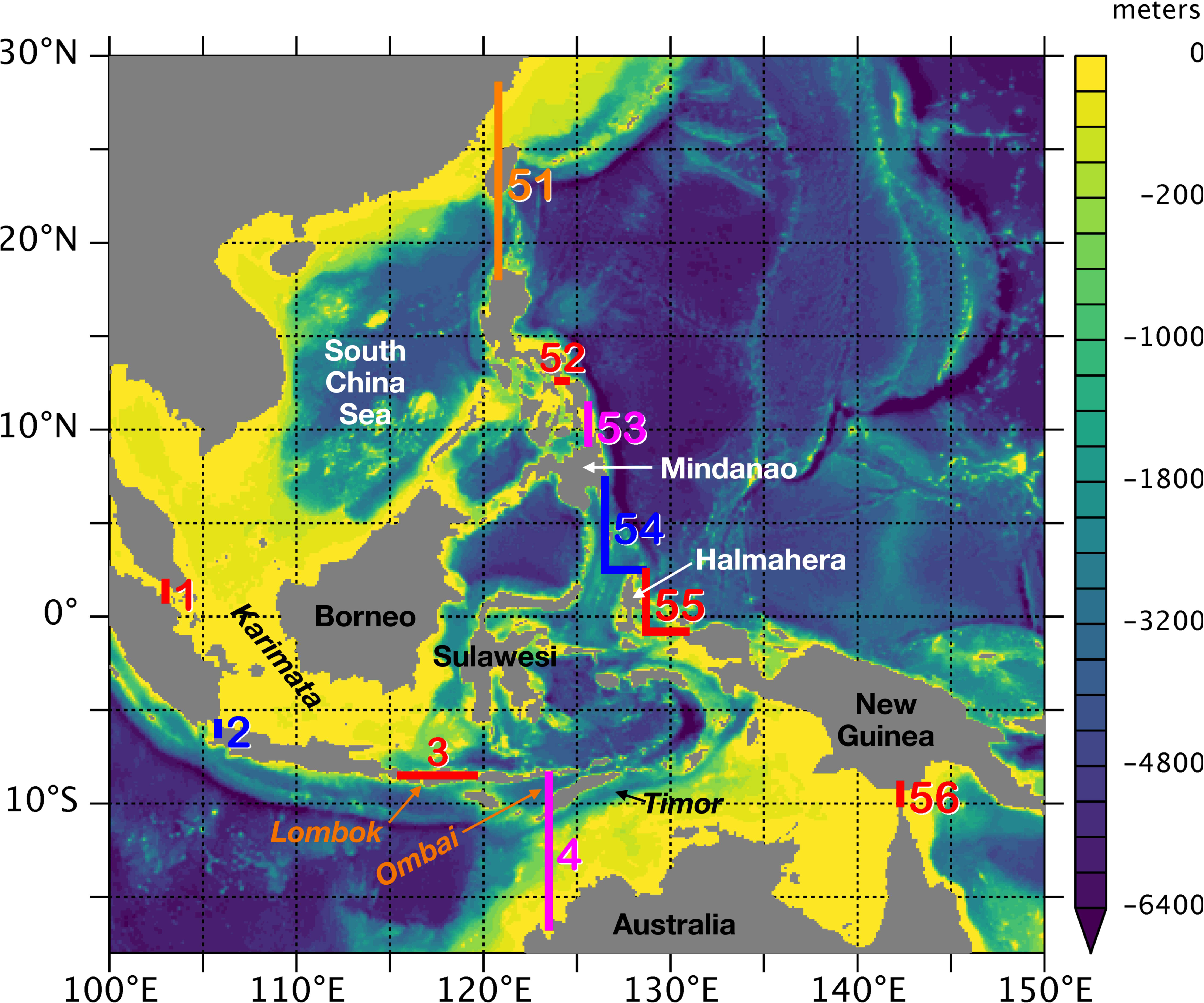
Figure 1 Geographical names, transects used to calculate ITF transports (thick lines), and bottom topography from the OGCM (meters, shading). The contour interval for bottom topography is 50 m for the upper 200 m, 200 m from 200 to 2,000 m depth, and 400 m thereafter. The slanted font indicates straits. The largest three contributors to the ITF transport on the Indian side are Lombok Strait (included in transect 3) and Ombai Strait and Timor Passage (included in transect 4). See Table 1 for the definitions of the transects.

Pacific water enters the Indonesian Seas through various channels between the islands of Mindanao, Halmahera, and New Guinea. A large fraction, ~12 Sv, of this transport then goes through Makassar Strait between the islands of Borneo and Sulawesi (e.g., Feng et al., 2018); this is the “western route.” The rest flows east of Sulawesi; this is the “eastern route”. The annual-mean volume transport through the South China Sea (from the Pacific, into the South China Sea, through Karimata Strait, into the Indonesian Seas, and then into the Indian Ocean) is small; estimates vary from 0.3 to 1.6 Sv (He et al., 2015).

The volume of water from the Pacific then flows into the Indian Ocean, with a large fraction of the annual mean transport, ~12 Sv, passing through Ombai Strait and Timor Passage, and the rest passing through Lombok Strait. The other narrow and shallow straits appear to be negligible in terms of annual mean volume transport.

The long-term-mean barotropic transport can be explained by wind stress in the Pacific via a linear Sverdrup theory (Godfrey, 1989), as potentially modified by friction and bottom topography (Wajsowicz, 1993). Linear wave dynamics can largely explain the vertical structure of the annual mean ITF (McCreary et al., 2007). The interannual variability has been associated with El Niño–Southern Oscillation (e.g., Feng et al., 2018).

1.2 Intrinsic variability

On the other hand, large-scale oceanic flow is known to include intrinsic (chaotic) variability. The reader is referred to Kalnay (2002, Section 6.4 of her book) for a full discussion or to Shukla’s (1998) Introduction for a concise review of this issue. (See also the informal discussion in Supplementary Section S1.1.).

Even though the oceanic flow follows deterministic dynamics in principle, some aspects of it are extremely sensitive to initial conditions. That is, two integrations of an identical ocean model, starting from almost-identical initial conditions and being driven by identical forcing and identical boundary conditions, can develop into appreciably different states. Such a phenomenon is called “chaos” and the ocean is a chaotic system.

Mesoscale eddies are an obvious and trivial example. Since they are generated by instability, they are not perfectly predictable. In particular, their phases are random, even if their statistical properties (e.g., mean eddy kinetic energy) are ultimately determined by external forcing and boundary conditions. Less obvious examples include the interannual and decadal variability of the Kuroshio Extension (KE). Nonaka et al. (2016, 2020) found that some properties of the KE differ between multiple runs of an ocean general circulation model (OGCM) started from just slightly different initial conditions.

For a chaotic system, a model prediction and the reality can be different even if the model were perfect and the forcing and boundary conditions were perfectly accurate because there is always some uncertainty in the initial condition. Because of this insurmountable uncertainty, we often view our system as partially probabilistic and call this conceptual difference between multiple runs or “realizations,” “intrinsic variability.” This variability is not temporal; it is variability in the probabilistic dimension (e.g., Farmer, 1982, his/her Introduction). The variability obeys a probability distribution. Since the probability density function is not known a priori, we often run a numerical model multiple times with slightly different initial conditions. Such an “ensemble” of runs is used to explore the probabilistic aspect of the oceanic flow. (See also the informal discussion in Supplementary Section S1.2.).

1.3 This study

Chaos poses an interesting question about the sensitivity of the oceanic flow to various parameters. For example, Sasaki et al. (2018) found a long-term increasing trend in the ITF transport after a tidal mixing parameterization was introduced. Could part of this trend be an intrinsic variability triggered by the parameter change (Lima et al., 2019; see also Supplementary Section S1.3)? To answer this question, the size and other statistical properties of the intrinsic variability have to be known.

In the present study, we explore the probabilistic dimension of the ITF transport using the 10-member ensemble of Nonaka et al. (2020). The purpose of the present study is to document the intrinsic variability associated with ITF transport. Since the ITF is essentially determined by large-scale winds (e.g., Godfrey, 1989; Wajsowicz, 1993), it is interesting to see if the ITF includes intrinsic variability at all.

The rest of the paper is organized as follows: Section 2 describes the ensemble of model runs to be analyzed and the methods of analysis. Section 3 shows the results: it first describes the intrinsic variability of the total, annual mean ITF transport; explores the vertical profiles of the variability, followed by the regional horizontal distribution; and then explores the basin-scale extent of the variability. Finally, Section 4 summarizes the results, and then, on the basis of the results, it proposes a hypothesis about the mechanism of the intrinsic variability for future studies to test.

2 Data and methods

2.1 OGCM ensemble data

The OGCM we use is a variant of MOM3 (Pacanowski and Griffies, 2000) called OFES2 (Sasaki et al., 2020; https://www.jamstec.go.jp/ofes/). It has been integrated from 1958 to 2021. The horizontal resolution is 0.1° × 0.1°, and the vertical resolution ranges from 5 m near the surface to 300 m near the bottom, with 105 levels in total. The computational domain is from 76° S to 76° N, and along these artificial boundaries, temperature and salinity are restored to the monthly climatological values from World Ocean Atlas 2013 version 2 (WOA13v2; Locarnini et al., 2013; Zweng et al., 2013).

The surface fluxes are calculated on the basis of an atmospheric data product, JRA55-do (Tsujino et al., 2018), which is based on a re-analysis. The surface momentum flux is calculated with Large and Yeager’s (2004) bulk formula using the wind velocity relative to the surface ocean current. The surface heat flux and evaporation are also calculated with Large and Yeager’s (2004) bulk formula on the basis of the re-analysis data. The precipitation is used as given by JRA55-do, and river runoff is specified according to another product. A sea–ice submodel is incorporated (Komori et al., 2005). Freshwater flux due to precipitation, evaporation, river runoff, and sea–ice formation or melting is all converted to virtual salt flux, and, as a result, there is no flux of volume through the sea surface. In addition to this salt flux, the sea-surface salinity is weakly restored toward the monthly climatological values from WOA13v2.

A 10-member ensemble is created, starting from the beginning of the year 1965 (Nonaka et al., 2020): specifically, the initial ocean state for 1 January 1965 is replaced with those of the 3rd, 5th,…, and 21st of January 1965 of the standard run, whereas the forcings and boundary conditions still start from 1 January 1965. The model is then integrated up to the end of 2016. The 10 runs thus obtained are called $m=1$, $m=2$, …, and $m=10$ in this study. We use the monthly mean output of the model for the period 1976 to 2016, which is 41 years. Past studies on the same dataset (Nonaka et al., 2020; Furue et al., 2021) suggest that after 5–10 years from the start (the year 1965), the ensemble spread does not systematically increase. The ensemble anomaly shown below in this study does not systematically increase, either. It is therefore likely that the ensemble statistics are stationary in the present dataset (1976–2016). Note that there is no guarantee that these “samples” are statistically unbiased. It is possible that, however many runs we make by perturbing the initial condition as described above, the density of the solutions in the probability space may not be proportional to the true probability density function.

2.2 Methods

2.2.1 Ensemble anomaly

Any variable in our study can in general be denoted by

$$\gamma (ȷ,l,m)\text{\hspace{1em}or\hspace{1em}}\gamma (ȷ,t,m)$$

where $ȷ=1,\dots ,N$ is a serial number of the gridpoints at which the variable is defined, $l=1,\dots ,L$ is the time index, and $m=1,\dots ,M$ is the ensemble-member number. We sometimes use time $t$ instead of index $l$ and write, e.g., $t=1986$ to denote the year 1986. The ensemble anomaly is naturally

$\begin{array}{ll}\tilde{\gamma }(ȷ,l,m)\equiv \gamma (ȷ,l,m)-\frac{1}{M}{\sum }_{m=1}^M\gamma (ȷ,l,m).& (1)\end{array}$

2.2.2 Linear regression

We calculate the linear regression coefficient between the ensemble anomaly of the annual mean ITF transport, $\tilde{q}(l,m)$, and some variables, $\tilde{\gamma }(ȷ,l,m)$, to be named in Section 3. Details are found in Appendix A.1. Linear regression extracts two parts from $\tilde{\gamma }$ as

$\begin{array}{ll}\tilde{\gamma }(ȷ,l,m)=\alpha (ȷ)\tilde{q}(l,m)+{\tilde{\gamma }}^{\text{′′}}(ȷ,l,m)& (2)\end{array}$

at each $(l,m)$, where $\alpha (ȷ)$ is the regression coefficient at gridpoint $ȷ$ and ${\tilde{\gamma }}^{\text{′′}}(ȷ,l,m)$ is the residual. The term $\alpha (ȷ)\tilde{q}(l,m)$ is that part of $\tilde{\gamma }$which is maximally correlated with $\tilde{q}(l,m)$ and ${\tilde{\gamma }}^{\text{′′}}(ȷ,l,m)$ is the part which is uncorrelated. In Figures 7, 8 below, we compare $\tilde{\gamma }(ȷ,l,m)$ with $\alpha (ȷ)\tilde{q}(l,m)$, not only in terms of the spatial pattern but also in terms of values. If the two fields are similar, that is an indication that the correlated part dominates at the particular $(l,m)$.

Note that this statistical calculation critically depends on the “degrees of freedom,” which are at most LM − L because there are L constraints that the ensemble average of the data is zero at each year (Walker, 1940). If each annual mean is statistically independent between years and between members, this is the actual degrees of freedom. To try to find other internal dependency than the $L$ constraints, we have calculated the temporal autocorrelation of $\tilde{q}(l,m)$ for all members combined (Supplementary Figure S2; see also Section 3.1) and found that the correlation is small for lags of 1 year and larger. This suggests that ensemble anomalies may be independent year to year. This conclusion, however, is tentative, and we acknowledge that the degrees of freedom of LM − L can be an overestimation. [There is indeed some hint of spectral peaks (Section 3.1), which, if real, suggests an overestimation.] The statistical significance of the regression coefficients we show below is based on the assumption of degrees of freedom of LM − L, but the significance could be an overestimation as a result.

2.2.3 Ensemble–temporal EOFs

We also use empirical orthogonal functions (EOFs) to explore characteristic spatial patterns of ensemble anomalies. Details are found in Appendix A.2. EOFs are orthogonal to each other; in other words, the spatial correlation between any two EOFs vanishes. From this property, the original variable, $\tilde{\gamma }(ȷ,l,m)$, can be expanded in terms of EOFs as

$\begin{array}{ll}\tilde{\gamma }(ȷ,l,m)={\displaystyle \sum _n}{\varphi }_n(l,m)e_n(ȷ),& (3)\end{array}$

where $e_n(ȷ)$ is the $n$th EOF, commonly termed “EOF$n$”, and ${\varphi }_n(l,m)$ is the coefficient of expansion, often called the $n$th “principal component”.

From the orthogonality of EOFs, we can derive (Appendix A.2)

$\begin{array}{ll}\text{variance at }(l,m)={\displaystyle \sum _n}{\varphi }_n^2(l,m),& (4)\end{array}$

$\begin{array}{ll}\text{overall variance}={\displaystyle \sum _n}\sum _{l,m}{\varphi }_n^2(l,m).& (5)\end{array}$

The EOFs are customarily numbered in the order of decreasing contribution to the overall variance:

$$\sum _{l,m}{\varphi }_1^2(l,m)>\sum _{l,m}{\varphi }_2^2(l,m)>...$$

by definition. On the other hand, the order of contribution, ${\varphi }_n^2$, is generally different at each $(l,m)$; for example, see Figure 6 below.

In Figure 6 below, we compare $\tilde{\gamma }(ȷ,l,m)$ with ${\varphi }_n(l,m)e_n(ȷ)$ for a particular mode $n$ or for the sum of two modes, not only in terms of the spatial pattern but also in terms of values. If the two fields are similar, that is an indication that the particular EOF mode(s) dominate(s) at the particular $(l,m)$.

2.2.4 Calculation of ITF transports

Figure 1 shows the transects across which transports are calculated, and the definitions of the transects are listed in Table 1.

TABLE 1

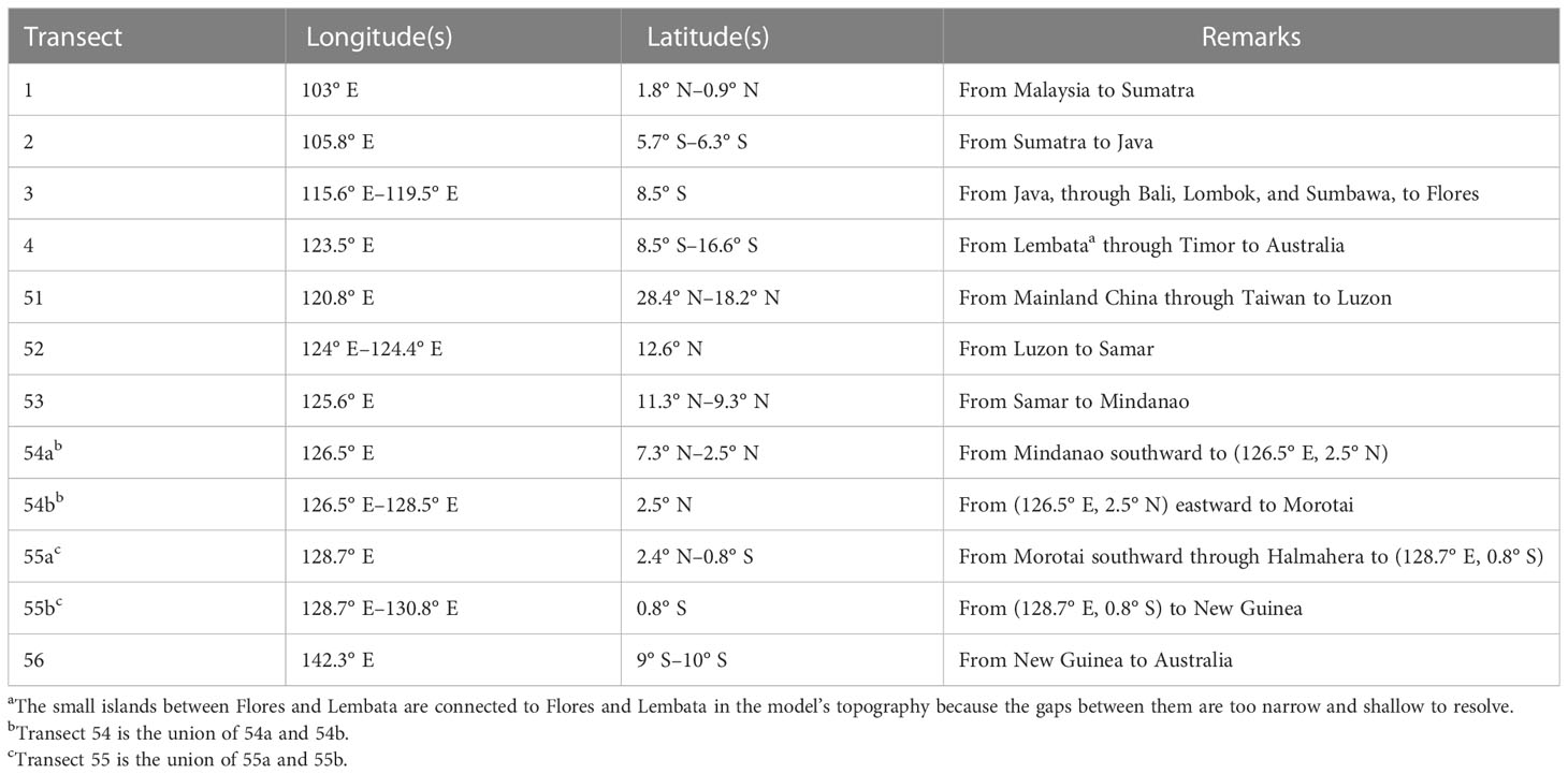
Table 1 Transects to calculate transports.

These transects are designed to completely enclose the Indonesian Seas in the model, where some of the shallow, tiny gaps between some islands have already been closed. We mainly use the four transects (1 through 4) on the Indian Ocean side to calculate the total ITF transport. We have also calculated the total ITF transport on the Pacific side and found that, on annual average, the total transport differs by 0.02–0.05 Sv and sometimes up to 0.07 Sv (not shown), indicating that the barotropic flow has little divergence or convergence at this time scale, as expected. The small error must be because we ignore the variability of sea level in the calculation of transports: If there is a correlation $\overline{u^{\prime }{\eta }^{\prime }}$ between the horizontal and temporal variabilities of horizontal velocity $u$ near the surface and sea level $\eta$, where the overline denotes the temporal average and average along the transects, this volume flux counts toward the error. For an order-of-magnitude estimate, let us suppose that $\eta \sim 0.5 \text{m}$, $u\sim 0.1 \text{m}/\text{s}$, and $\text{length\hspace{0.17em}of\hspace{0.17em}transect}\sim 1,000 \text{km}$, which gives a transport of 0.05 Sv, not inconsistent with the volume imbalance. Since the model uses a Boussinesq approximation (Pacanowski and Griffies, 2000), volume is perfectly conserved (Section 2.1), and therefore the only other potential source of imbalance is the area-integrated sea-level change (${\int }^{}dxdy\overline{\partial \eta /\partial t}$), which must be on the same order or less.

We first integrate along the transect the velocity component normal to it

$$\mathcal{V}(z,t;m)=\{\begin{array}{ll}{\int }_{y_s}^{y_n}dyu(x=x_t,y,z,t;m)\hfill & \text{or}\hfill \\ {\int }_{x_w}^{x_e}dxv(x,y=y_t,z,t;m),\hfill & \hfill \end{array}$$

depending on the orientation of the transect, where $x_t$ or $y_t$ is its longitude or latitude. For transects 54 and 55, each of which consists of a meridional and a zonal segment, $\mathcal{V}$ is the sum of the zonal and meridional transports.

This integral gives the volume transport per unit depth across the transect as a function of depth. Upon vertical integration, it gives the total volume of transport across the transect. The sum of the transports for transects 1–4 is the total ITF transport on the Indian side and the sum over transects 51–56 is the total ITF transport on the Pacific side.

2.2.5 Pseudo-streamfunction

In addition to the transports across the transects, we calculate a barotropic streamfunction, $\psi$, defined as

$\begin{array}{ll}V={\psi }_x,U=-{\psi }_y,& (6)\end{array}$

where $U$ and $V$are the horizontal velocity components integrated from the bottom to the sea surface, and the subscripts indicate partial derivatives. Here, we use the Cartesian coordinates for simplicity, but we use the spherical coordinates for the actual calculation. This definition implies that when ${\psi }_x>0$ and ${\psi }_y=0$, for example, the barotropic current is northward: $V>0$ and $U=0$. When ${\psi }_x=0$ and ${\psi }_y>0$, the current is westward. In general, the barotropic circulation is clockwise around a local maximum of the streamfunction.

This definition implies that $U_x+V_y={(-{\psi }_y)}_x+{({\psi }_x)}_y=0$. Therefore, strictly speaking, the barotropic streamfunction does not exist because of small divergence or convergence. As described above, however, divergence and convergence within the Indonesian Seas are negligible on an annual average. It should also be small everywhere because barotropic adjustment should be fast.

For convenience, then, we use a “pseudo-streamfunction”: we first plug in zeros to the velocity variable at land grid points and then integrate $V$ in the zonal direction starting from a point in Australia, which determines the values of the streamfunction along this latitude circle. From each gridpoint on the circle, $U$ is integrated meridionally, determining the values everywhere on the sphere. Since we give zero velocity to land, streamfunction values are formally defined on land. As will be seen later, this arrangement is convenient to visualize transport between two landmasses. In particular, a western boundary current leads to a rapid zonal change in $\psi$, resulting in a maximum or minimum value right at the coast. Since the integration of $\psi$ is continued inland, the landmass acquires the same value as along its coast. If the landmass were masked out, the maximum or minimum value at the coast would be hard to see on the map of $\psi$.

3 Results

3.1 ITF transports

Figure 2A shows the annual mean total transport for all ensemble members. There is large interannual variation. The annual mean transport estimates from the INSTANT project (Table 1 of Gordon et al., 2010) are 14.0, 15.7, and 15.3 Sv for the years 2004–2006. In our model, the transport values are 13.4–14.1, 14.2–15.0, and 14.4–15.0 Sv for the same 3 years. For a longer time series, we have looked at the zonal transport estimates across the IX1 section between Fremantle and the Sunda Strait over 1984–2015 (Liu et al., 2015), plotting annual averages based on the dataset of Feng et al. (2018), and found that the year-to-year variation of the annual mean ITF transport ranges from 1 to 4 Sv (not shown). This range is consistent with that of OFES2 (Figure 2A). The time series of the total ITF transport do not agree (not shown) between the observation and our model. Apart from model error, the discrepancy may be partial because the observation is an estimate based on a repeated hydrographic survey in the upper ocean across the section further west and is therefore affected by the slower baroclinic adjustment timescales (M. Feng, private communication, 2022) and perhaps by other zonal flows than the main ITF westward outflow. As an indirect comparison with observation, the model ITF transport tends to be larger in La Niña years (Supplementary Figure S1), consistent with previous studies (e.g., England and Huang, 2005; Feng et al., 2018, and references therein).

FIGURE 2

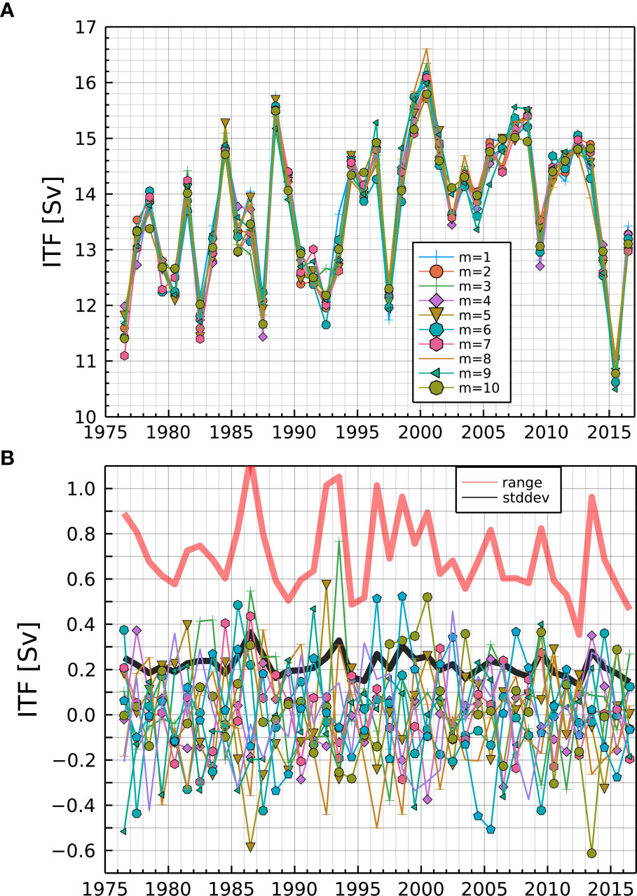
Figure 2 Annual-mean ITF transports for each of the 10 members ($m=1,\dots ,M$): (A) total and (B) ensemble anomaly. In (B), the thick pink curve is the difference between the maximum and minimum members for each year, and the thick black curve represents the ensemble standard deviation $(\sqrt{{\displaystyle {\sum }_m{\tilde{q}}_m^2/(M-1)}})$, where ${\tilde{q}}_m(t)$ is the ensemble anomaly for year $t$ of member $m$. The tic marks on the horizontal axis indicate the beginning of the year.

The ensemble anomaly (Figure 2B) is sometimes as large as 0.5 Sv, and the difference between the maximum and minimum members (thick pink curve) sometimes reaches 1 Sv. There is no obvious relation between the total transport (Figure 2A) and the ensemble spread (Figure 2B). At this point, one might wonder whether these ensemble anomalies could arise from numerical truncation errors in the OGCM’s code, but it would be highly unlikely that such error leads to the systematic variability shown in Sections 3.3–3.5 below.

The temporal autocorrelation of the annual mean ensemble anomaly for all members combined (Supplementary Figure S2) is not statistically significant at a 99% confidence level and barely exceeds the 95% confidence level at lags of 4 and 14 years. For this reason, we treat each annual mean ensemble anomaly value as independent. This does not necessarily mean that the ensemble spread dramatically decreases in averages over a few years. We have made similar plots to Figure 2 for the 2-year (not shown) and 3-year (Supplementary Figure S3) moving averages of the annual mean data. The difference between the maximum and minimum reaches above 0.6 Sv on several occasions, both in the 2- and 3-year-mean data. Even though (or even if) the year-to-year ensemble variability is statistically independent, it takes more than a few years to average out the statistical variability. The potential autocorrelation mentioned above will be briefly discussed later (Section 4.2).

3.2 Transport by transect

We next examine transports across various transects (Figure 1). On the Indian side, the main channels are the Lombok and Ombai Straits and Timor Passage (Gordon et al., 2010). The transport numbers from the INSTANT project (Gordon et al., 2010, their Table 1) are 12.0, 13.4, and 11.9 Sv for the years 2004, 2005, and 2006 for Ombai Strait and Timor Passage combined. This transport is captured by transect 4 of our model, which is 10.8, 11.8, and 11.5 Sv for those 3 years on ensemble average. Similarly, Lombok Strait gives 2.0, 2.3, and 3.4 Sv in Gordon et al. (2010), while transect 3, to which Lombok Strait is by far the dominant contributor, gives 2.7, 2.6, and 3.0 Sv.

Figure 3 shows a breakdown, by transect, of annual mean transport for the year 1986, when the difference between the maximum and minimum members is largest (Figure 2B). For comparison, the third bar (green) shows the average over all members and over the entire period. The difference between the maximum and minimum members is about 10% for transect 4, whereas it is about 3% for transect 3. In the other years (not shown), the difference between the maximum and minimum members is always very small for transect 3. The transports across the other two channels are negligible not only in 1986 but also in all other years (not shown). We, therefore, focus on transect 4 in the following analysis.

On the Pacific side, the mean transport is the largest for transect 54. The difference between the maximum and minimum transports is also the largest for the same transect during 1986 (Figure 3); this property applies to all the years (not shown). As an aside, the transport across transect 55 varies between about −2.5 and 2 Sv (not shown), with positive values indicating inflow into the Indonesian Seas.

FIGURE 3

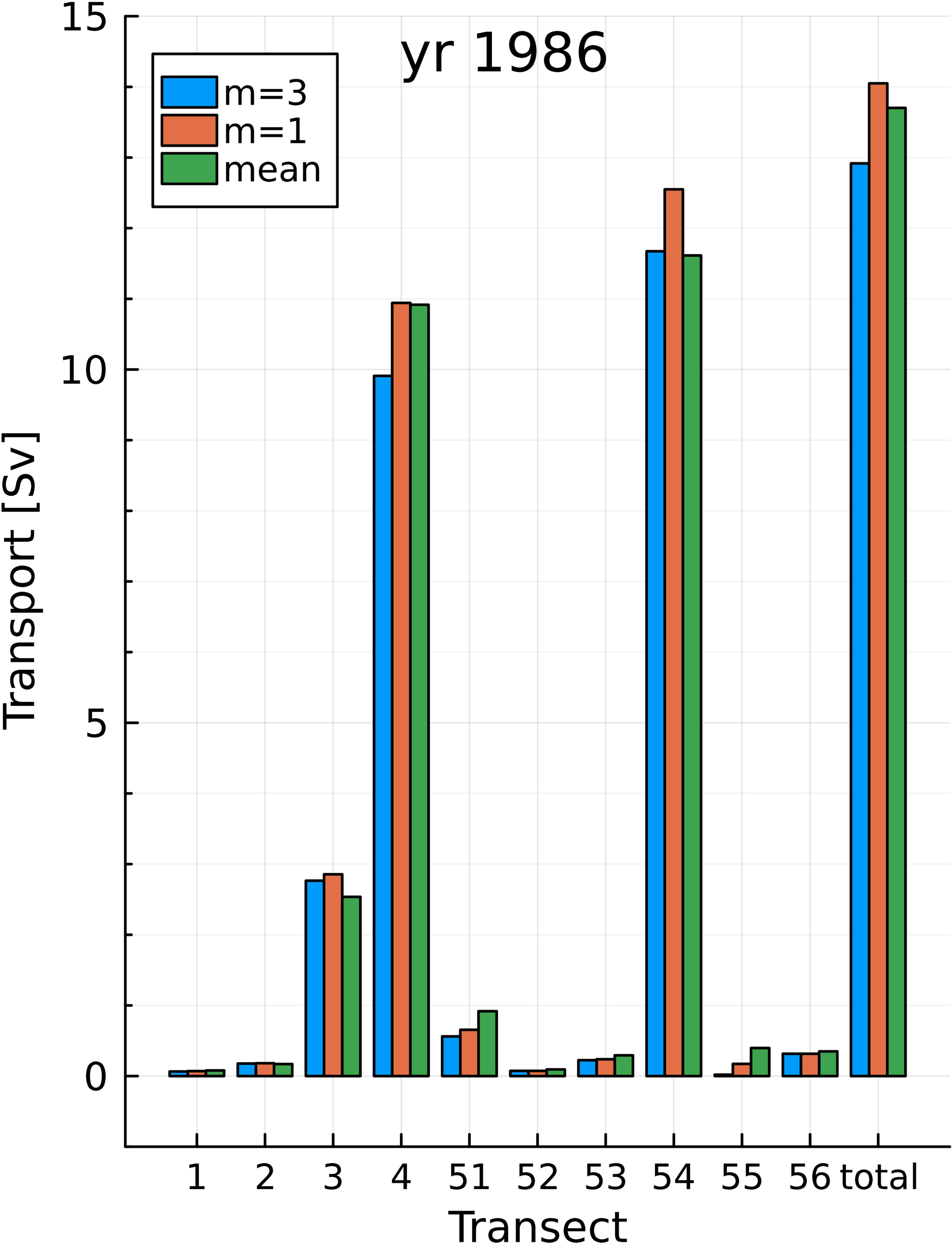
Figure 3 Breakdown of ITF transport by transect. The horizontal axis indicates transect numbers (Figure 1) except that the last column indicates the total ITF transport on the Indian side. The blue and red bars are for members $m=1$ and $m=3$, which have the minimum and maximum total ITF transports for the year 1986, when the difference between the minimum and maximum ITF transports is largest (Figure 5B). The green bar shows the average over all members and over the entire period, not just 1986. All transport numbers are in Sverdrups, with positive numbers indicating a transport into the Indian Ocean (for transects 1–4) or into the Indonesian Seas (for transects 51–56).

3.3 Vertical structure

3.3.1 Ensemble anomaly

Figure 4 shows the vertical profiles of horizontally integrated, cross-sectional anomalous velocity, $\tilde{\mathcal{V}}(z;t,m)$, for transects 4 and 54 (Section 2.2.4); the transport values quoted earlier are the vertical integrations of this quantity.

FIGURE 4

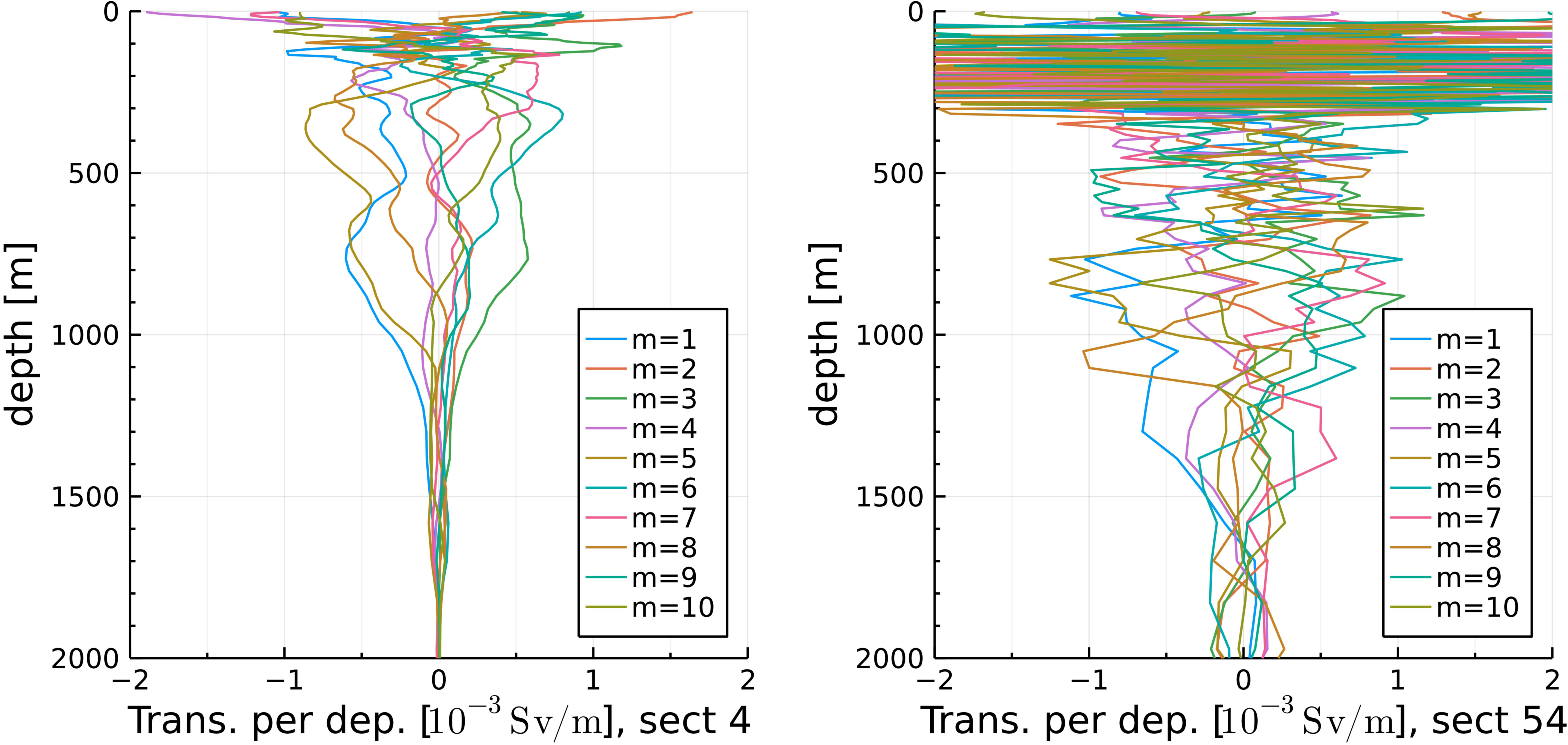
Figure 4 The vertical profiles of horizontally integrated anomalous velocity, $\tilde{\mathcal{V}}(z;t,m)$, across transects 4 (left) and 54 (right) for $t=1986$ and for all $m\text{'}$s.

In both transects, the profiles are very noisy above 200 and 300 m on the Indian and Pacific sides. The high-wavenumber structure is particularly prominent in transect 54. We have examined several instances of the meridional–depth section of annual-mean zonal velocity along this transect (not shown) and found that the noisy feature above 300 m is located near the northern end of the transect, that is, near the coast of Mindanao (Figure 1). It is interesting that such a high-wavenumber feature remains on an annual average.

In contrast, no particularly noisy features are visible in the meridional–depth plots we examined (not shown) along transect 4; the wiggliness in the upper ocean is due to the horizontal integration of features with various vertical scales and structures. This difference could be because transect 4 is quite far from the actual narrow channels (Ombai and Timor).

3.3.2 EOFs

Below this surface layer, the vertical structure appears more systematic, especially in transect 4. We here calculate EOFs (Section 2.2.3) of $\tilde{\mathcal{V}}(z;t,m)$.

Figure 5 shows the gravest five EOF modes for transects 4 and 54. The noisy near-surface layer is excluded from the calculation. For transect 54, the top 320 m is excluded. When the threshold was 300 m (not shown), one of the gravest modes peaked at 300 m, likely because it still caught the variability of the near-surface layer. The lower bound is set at 2,200 m, below which the EOF modes tend to vanish for both transects.

The EOF modes tend to have smooth vertical profiles. EOF1 does not change signs and has a vertical transport, whereas the other modes are baroclinic, reminiscent of the vertical dynamical modes associated with baroclinic waves. For transect 4, EOF1 is clearly dominant, whereas for transect 54, power goes down more slowly with increasing mode number.

Potemra et al. (2003) obtained EOF modes for the vertical profiles of the volume transports across Ombai Strait and Timor Passage in a 20-year integration of an OGCM. One of their gravest two modes (their Figure 6) is surface-intensified and nearly zero below 400 m. The other mode peaks at 400 m and vanishes below 800 m in Ombai or peaks at 200 m and vanishes below 600 m in Timor, with a weaker reverse flow in the top 100 m. The time series (principal components) of both modes include large interannual variability (their Figures 6e, f). These modes stay essentially the same after the removal of annual and semiannual harmonics. Our EOFs for transect 4 (Figure 5, left panel) miss these modes, all of which have multiple peaks below 400 m, either because we omit the top 200 m or because our variability is of different nature. It would not be surprising if the latter is the case because our data is a deviation from the ensemble average, not a temporal variability originating directly from external forcing.

FIGURE 5

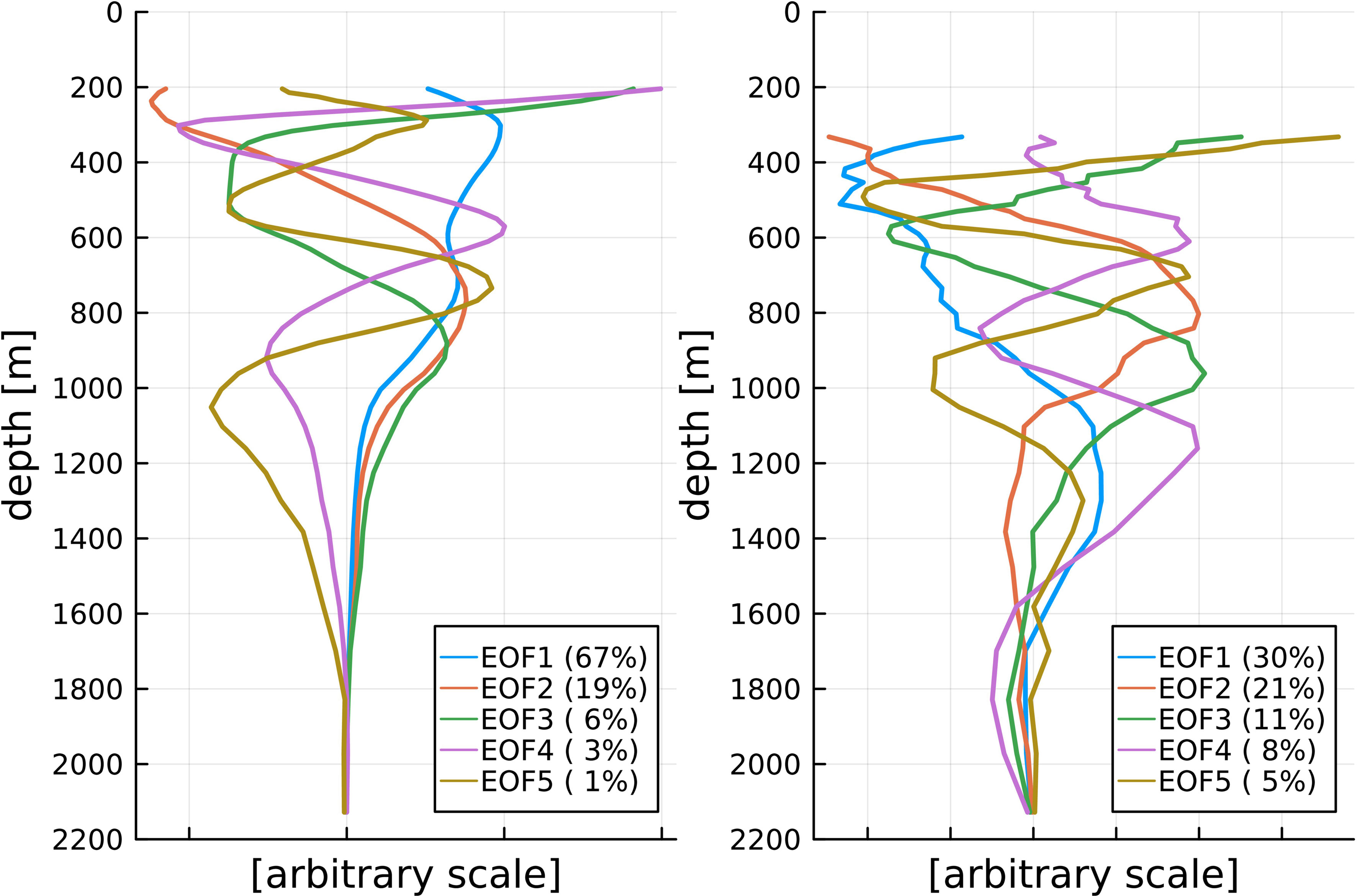
Figure 5 EOF modes of $\tilde{\mathcal{V}}$ (Figure 4) for transects 4 (left) and 54 (right). The horizontal axis has arbitrary units. The top 200 and 320 m are excluded from the calculations. The lower limit is set at 2,200 m for both transects. The percentage numbers in the legend indicate the contribution of each mode to the total variance (see 4b).

The upper panels of Figure 6 compare $\tilde{\mathcal{V}}(z,t;m)$ with the vertical profiles, [${\varphi }_n(t,m)e_n(z)$] of EOF modes, for $t=1986$, for $m=1$ and $m=3$, and for transect 4. In both members, EOF1 dominates while the second contribution, which is below 10%, comes from different modes. For all the top 5 years with large transport differences (1986, 1992, 1993, 1996, and 2013; see Figure 2B), EOF1 is the dominant mode with a 70% contribution or larger except for $t=1993$ and $m=3$, where EOF1 has only 42% and EOF1 + EOF2 has 76% (Supplementary Figure S4). That is, EOF1 has a large amplitude and explains a large part of the vertical profile when the ITF ensemble anomaly is large, at least for the 5 years we have examined.

FIGURE 6

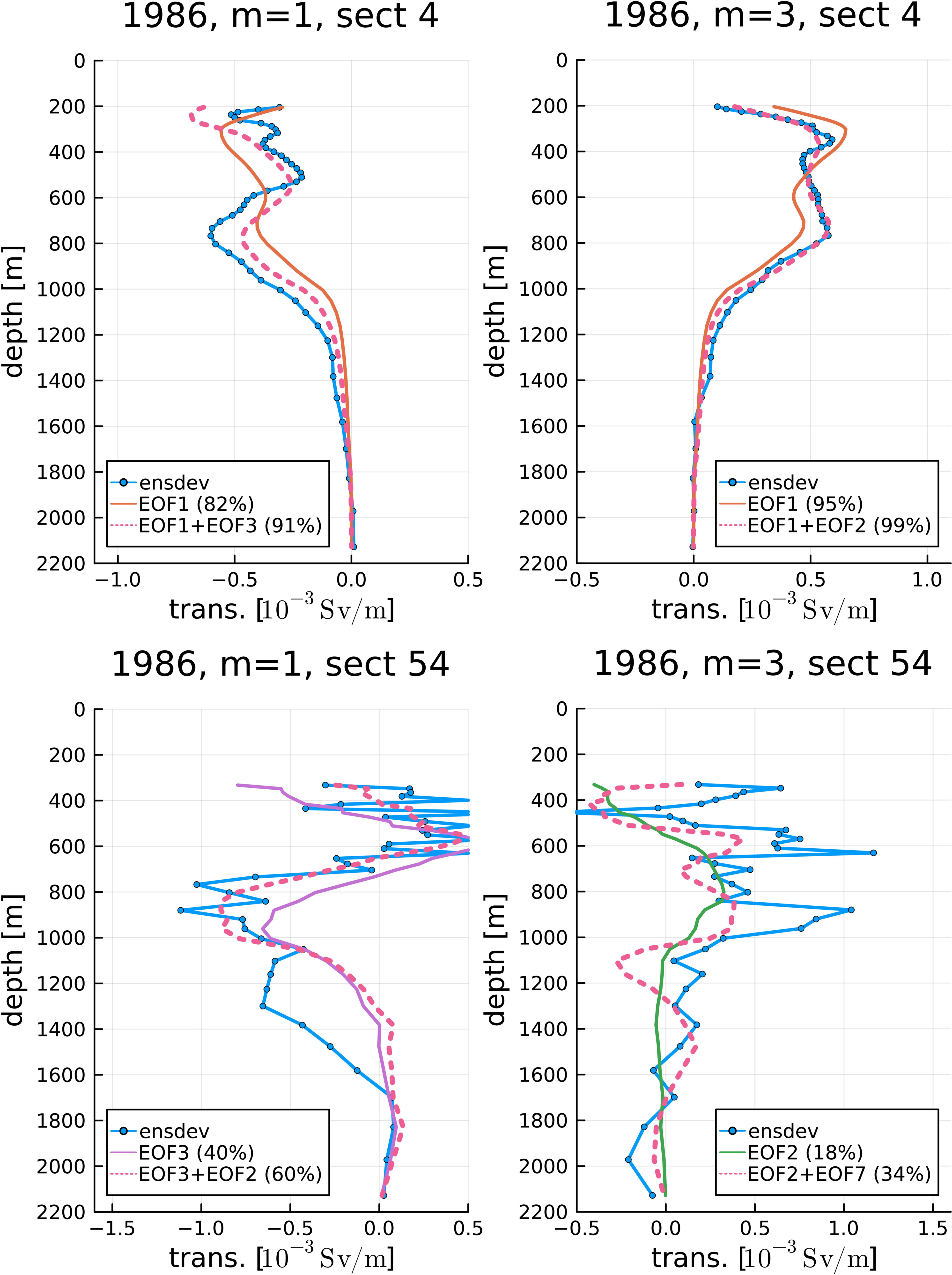
Figure 6 Vertical distribution of transports for 1986, transects 4 (upper) and 54 (lower), and $m=1$ (left) and $m=3$ (right). The solid curve with symbols represents the original transport; the solid curve without symbols represents the EOF mode that has the largest contribution for the year and member; and the dashed curve represents the sum of the top 2 EOF modes. See (3) and (4a).

On the Pacific side, however, EOFs 1, 3, 4, and 9 have the largest contributions (see Supplementary Figure S4 for an example where EOF4 is the largest) at one of the top 5 years for the maximum and minimum members, and even the sum of the top 2 modes sometimes explains only approximately 35% of the variance (not shown). EOF1 is baroclinic, without much horizontal transport. There are large intrinsic variabilities at the entrance to the Indonesian Seas that are not directly related to large ITF transport anomalies. The lack of particularly dominant modes on the Pacific side might be because of the direct impacts of the western boundary current or other coastal currents. It is interesting that even an annual mean and meridionally integrated velocity (blue curves in Figure 6) includes extremely high-wavenumber features.

3.3.3 Linear regression

While EOFs describe intrinsic variability itself, they do not necessarily describe the intrinsic variability associated with the intrinsic variability of the ITF transport as in the case of transect 54. For transect 4, EOF1 does seem to be correlated with the ITF transport anomaly, but we looked at only the top 5 years of large ensemble spread. Here, we calculate the linear regression coefficient which extracts the component of the intrinsic variability which is linearly correlated with the total transport of the ITF, $\tilde{q}(t,m)$.

Figure 7 shows the part of $\tilde{\mathcal{V}}(z;t,m)$ that is linearly correlated with $\tilde{q}(t,m)$ for $t=1986$ and $m=1$ and $m=3$. See Section 2.2.2 for the method. The linear model approximately matches the actual profiles, particularly well below 600 m depth on the Indian side, whereas the actual flow is much more complicated on the Pacific side than the linear model, again suggesting that variability not related to the ITF variability contributes much more at the entrance into the Indonesian Seas than after the exit. The regression coefficient, $\alpha (z)$, has a similar vertical structure to $\text{EOF}1(z)$ on the Indian side with a double peak at 300 and 700 m. This result strongly suggests that the dominant variability ($\text{EOF}1(z)$) is the one associated with the variability of the total ITF transport. It is interesting to note that on the Pacific side, the component of $\tilde{\mathcal{V}}(z;t,m)$ that is correlated with the total ITF transport has a smooth vertical profile below the near-surface noisy layer.

FIGURE 7

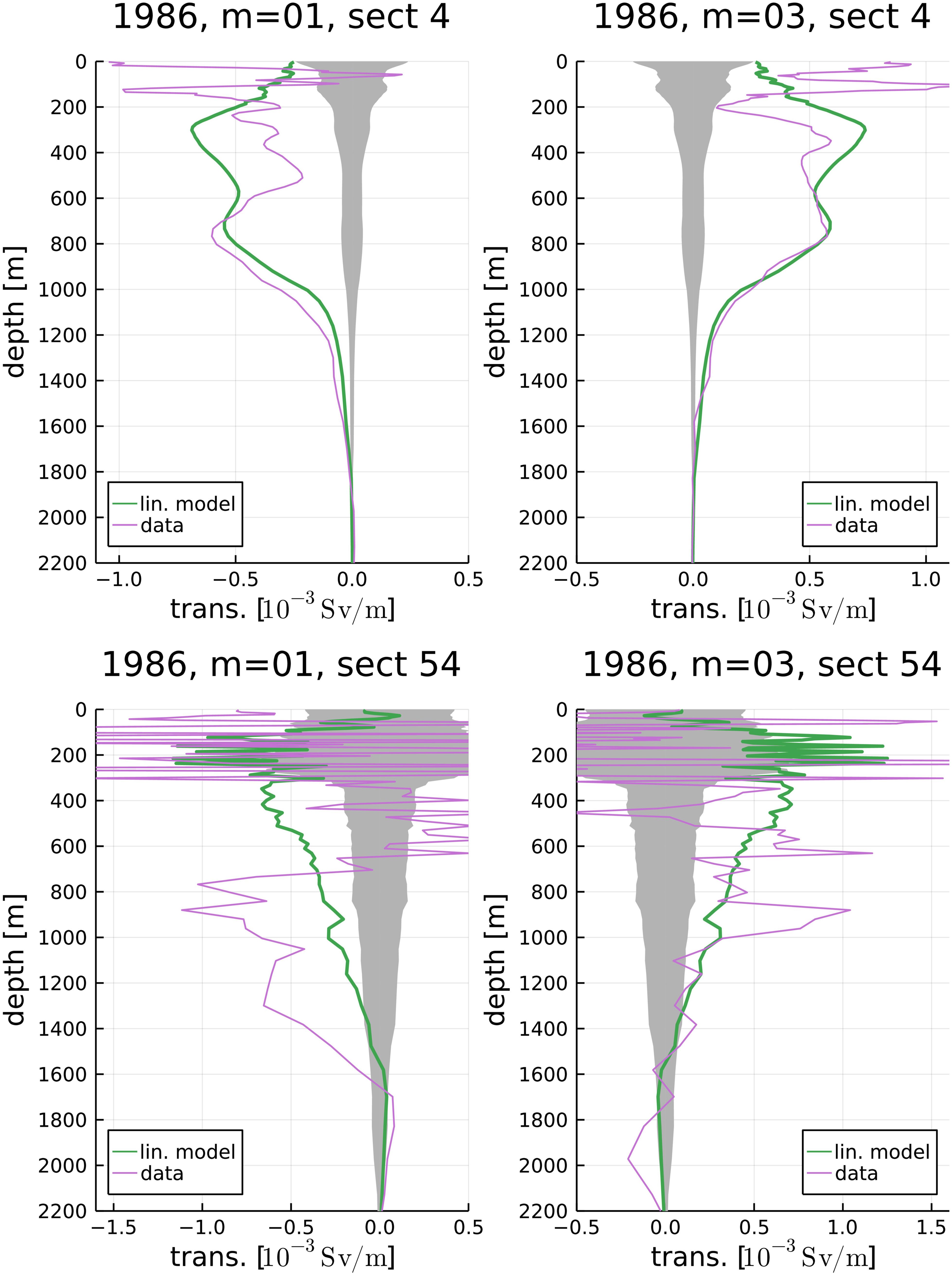
Figure 7 Vertical distribution of transports for 1986, transects 4 (upper) and 54 (lower), and $m=1$ (left) and $m=3$ (right). The thin violet curve shows the original transport anomaly, $\tilde{\mathcal{V}}$; the thicker green curve shows the linear model. The gray shading indicates an estimated threshold beyond which the linear model result is statistically significant with a confidence level of 99%. See Section 2.2.2.

Also, it is interesting that some of the peaks in $\alpha (z)$ in the near-surface noisy layer lie above the significance threshold (lower panels of Figure 7). The anomalous velocity itself (purple curves) includes very high-wavenumber features down to ~1,000 m. The depths of some of the peaks in the purple curve agree with those of the peaks in the regression (green curve) in the upper 300 m. It would be surprising if this noisy feature, also in Figure 4, is really correlated with the ITF transport. If it is real, it might be due to the western boundary current or other coastal currents acting on the coast of Mindanao. This issue may be an interesting subject of future study.

3.4 Horizontal structure

Figures 8A, B show the ensemble anomaly of the barotropic streamfunction, $\tilde{\psi }(x,y;t,m)$, which is higher or lower by about 0.5 Sv on the Eurasian continent for $m=1$ or $m=3$ in 1986 than on Australia, as expected because the difference in $\psi$ values between two points is equal to the barotropic transport across the line segment that connects the two points and because $\tilde{q}\approx \pm 0.5$ Sv for $m=1,3$ in 1986 (Figure 2B).

The Indian Ocean is dominated by large and noisy intrinsic variability, and the Pacific has zonally elongated stripes of large amplitude. In contrast, the anomalous flow field within the Indonesian Seas is relatively smooth and shows an increased ($m=1$) or decreased ($m=3$) ITF transport both in the eastern and western routes. This pattern is common to all the 5 large-ITF-difference years (not shown). This result suggests that the ensemble anomaly in the ITF transport is not a local phenomenon at the narrow channels in the Indonesian archipelago but an overall strengthening or weakening of the regular classical ITF as a whole.

Figures 8C, D show the part of $\tilde{\psi }$ which is linearly correlated with $\tilde{q}$ (Section 2.2.2), $\alpha (x,y)\tilde{q}(t,m)$, for $t=1986$ and for $m=1$ and $m=3$. The anomalous field $\tilde{\psi }$ largely agrees with $\alpha (x,y)\tilde{q}(t,m)$. This agreement indicates that the large-scale pattern in the ensemble anomaly (Figures 8A, B) is correlated with $\tilde{q}$.

FIGURE 8

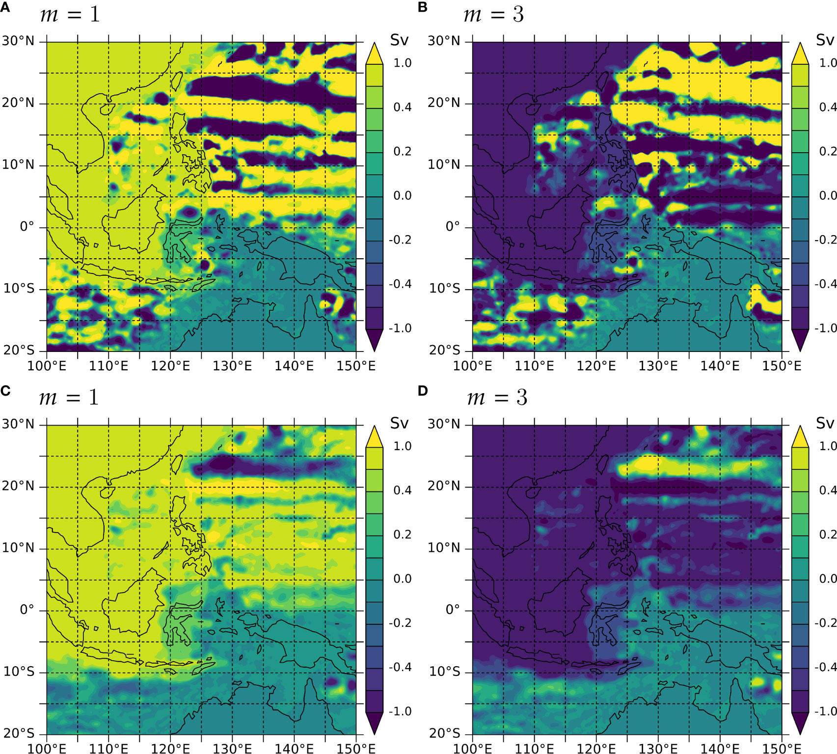
Figure 8 (A, B) Ensemble anomaly of barotropic streamfunction, $\tilde{\psi }(x,y;t,m)$, for $t=1986$ and for $m=1$ and $m=3$. (C, D) Linear regression of $\tilde{\psi }$ to $\tilde{q}$, $\alpha (x,y)\tilde{q}(t,m)$. Note that the contour intervals increase beyond $\pm 0.5$ Sv to de-emphasize stronger variability. Positive and negative values indicate, respectively, clockwise and counterclockwise circulation around extrema, and hence the positive and negative values on Eurasia indicate the strengthening and weakening of the ITF transport.

It is therefore likely that the intrinsic variability of the ITF is not a local phenomenon but is driven from the Pacific just as the mean ITF is driven by Pacific winds. The vertical structure of the regression coefficients in Figure 7 is probably that of this large-scale phenomenon.

3.5 Basin-scale view

3.5.1 Barotropic streamfunction

Figure 9 shows the regression coefficient between $\tilde{q}$ and $\tilde{\psi }$ this time using $\tilde{\psi }$ mapped onto a 0.5° × 0.5° grid to save computational efforts. Otherwise, the coefficient is the same as that plotted in Figure 8C. Again, we multiply the coefficient $\alpha (x,y)$ by the value of the ITF transport at $t=1986$ and $m=1$ to make the physical interpretation of the coefficient more convenient because with this multiplication, we can describe how the 0.5 Sv increase in the ITF transport above the ensemble average flows around the global ocean as below. If the ITF transport is 0.5 Sv below the average as in $m=3$ of $t=1986$, the signs should simply be flipped. If the amplitude of the increase or decrease is smaller, the streamfunction values below should simply be reduced by the same factor.

FIGURE 9

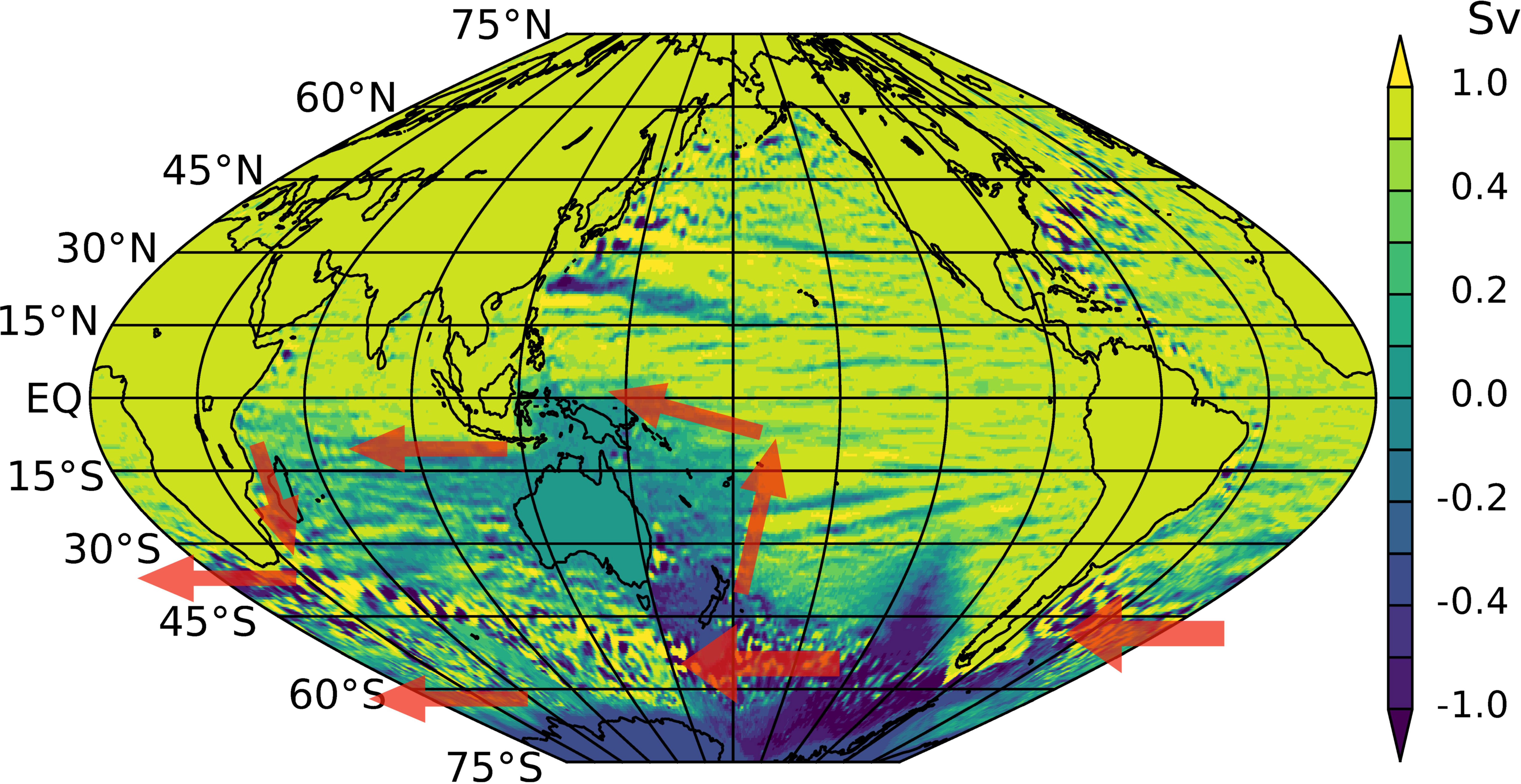
Figure 9 Streamfunction component maximally correlated with $\tilde{q}$ ($\alpha (x,y)\tilde{q}(t,m))$ at $t=1986$ and $m=1$. The arrows schematically represent the direction of the barotropic flow anomaly. See text.

The ITF transport anomaly has a robust correlation with streamfunction values on the continents, which is not surprising at all as streamfunction values on landmasses represent transports between the landmasses (Section 2.2.5). For this reason, estimates of statistical significance are not shown in this plot. Correlation is perfect on the continents and neighboring, relatively quiescent regions and is weak in other parts of the ocean only because of background noise. Moreover, the regression coefficient is always zero on Australia by definition and is very small in the region surrounding Australia, either (1) because the barotropic velocity is weak (and therefore the streamfunction values do not change much from the zero value of Australia) or (2) because of the background noise. Since small regression values are formally classified as nonsignificant, it is difficult to distinguish these two cases. For this reason, the statistical significance of simultaneous correlation makes sense only for values on landmasses.

The Eurasian continent has a value of about 0.5 Sv, which is equal to the ITF transport anomaly for $t=1986$ and $m=1$ (Figure 2B), which manifests itself as a westward transport between Australia and Eurasia. This transport, moreover, takes the form of a narrow flow along 10° S; that is, it takes the form of an increase in the South Equatorial Current in the Indian Ocean. This narrow flow is represented by the rapid northward increase in streamfunction values (equation 6), which agrees with the linear barotropic response (McCreary et al., 2007).

It is very interesting that the streamfunction value is negative (about 0.4 Sv) on Antarctica, which means that the transport anomaly is westward between Australia and Antarctica. Even though the correlation of $\tilde{q}$ with the Antarctic value of $\tilde{\psi }$ is well above the significance threshold (not shown), no clear pathway is visible in the Southern Ocean as the streamfunction values vary wildly at small spatial scales and the regression coefficient is under the 99% significance level. To obtain a clear mean pathway, we would need many more samples (ensemble members) to cancel out the noise.

In any case, combined with the 0.5 Sv increase in ITF transport, there is a westward transport anomaly of 0.9 Sv in the Indian sector, which flows westward south of Africa into the Atlantic sector of the Southern Ocean and then through the Drake Passage into the Pacific.

In the Pacific, the flow pattern is not clear because of the noisy streamfunction field, but the following description should be correct to satisfy the mass conservation. Most of this anomalous transport appears to bend northwestward to the west of South America and then flows back southwestward, circling the purple patch at ∼100° W, 45° S. It then continues westward again. Upon hitting New Zealand, 0.5 Sv bends northward along the Tonga–Kermadec arc and then bends northwestward to join the ITF; the rest flows south and joins the westward transport south of Australia.

McCreary et al. (2007) used an OGCM in a global domain without the Arctic Ocean and obtained a standard climatological solution. In a sensitivity solution, the Indonesian passages are closed at 8.5° S. The difference in the barotropic streamfunction between the two solutions shows a pure ITF. It flows westward along 10° S, and at Africa, it bends southward along the coast of Africa. Most of this flow bends eastward at the southern tip of Africa, forming a narrow eastward flow, and then bends northward at the southern tip of Tasmania, flowing along the east coast of Australia. Some of the transport, however, flows westward from the southern tip of Africa and eventually crosses the Drake Passage into the Pacific and eventually joins the northward flow along the east coast of Australia. This flow pattern is broadly similar to the ensemble anomaly of the streamfunction described above, except that the narrow eastward return flow that reaches Tasmania does not exist in our ensemble anomaly. The reason for the westward flow in the Southern Ocean is not clear, either in our result or in the result of McCreary et al. (2007). This potential connection of the net Southern-Ocean transport all around Antarctica with the ITF transport might be through some changes in overturning circulation similar to the change explored by Sen Gupta et al. (2016, their Supplementary Figure S10).

3.5.2 Lead-lag correlation

Lead-lag regression coefficients (Section 2.2.2) are also calculated (Figure 10). The figure shows only the North Pacific since there is no systematic and significant signal in other regions (Supplementary Figure S5) perhaps except for the potentially weaker stripes in the mid-latitude southern hemisphere. At lag 5 ($\text{Δ}t=-5$, $\tilde{\psi }$ leading $\tilde{q}$), there is a negative band extending southeastward from about 170° E, 30° N, and other positive and negative stripes south and southwest of it. There is another weaker negative band extending eastward from the south of Taiwan. As time goes on, this negative anomaly moves, together with the positive anomaly on its southern flank, westward and equatorward. Other lesser stripes appear to move similarly, but their motions are not as clear. At lag 1 ($\text{Δ}t=-1$), the strongest negative band reaches Okinawa and the associated positive band reaches Taiwan. At the same time, there is a negative band extending eastward from the southern tip of the Philippines. At lag zero (Figure 9), the major positive and negative bands are still visible, and the other lesser stripes are buried in the large-scale signal described above. At lag −1 ($\text{Δ}t=+1$, $\tilde{\psi }$ lagging $\tilde{q}$, Supplementary Figure S6), the negative band is still visible but much weaker extending from Taiwan, and there are no significant and systematic signals elsewhere, either.

3.5.3 Sea-surface height

The same analysis is carried out for sea-surface height (SSH). The simultaneous linear regression (not shown) is noisier than the corresponding linear regression on $\tilde{\psi }$ and provides similar information: SSH tends to be lower north of 10° S in the Indian Ocean, consistent with the westward barotropic transport there; SSH is higher near Antarctica, consistent with the westward transport in the Antarctic Circumpolar Current; and west of South America, there is a region of higher SSH coincident with the lower $\tilde{\psi }$ region there, consistent with the counterclockwise barotropic circulation there. On the other hand, SSH does not show the northward barotropic flow along the Tonga–Kermadec ridge (Figure 9). This difference may be an indication that the barotropic flow there is deeper, with less SSH signal, or that SSH “noise” is larger there.

Figure 11 shows a set of lead-lag regressions of the SSH anomaly on $\tilde{q}$ corresponding to that of $\tilde{\psi }$. The spatial pattern of the anomaly is very similar to that of $\tilde{\psi }$. The strong negative and positive bands of SSH that correspond to those of $\tilde{\psi }$ are particularly clear, and they migrate westward and equatorward. Other, lesser, stripes equatorward of this pair are also sometimes visible. The potential relation of these stripes in streamfunction and SSH to the ITF transport will be discussed below.

4 Summary and discussion

4.1 Summary

We have examined a 10-member ensemble of a semi-global ocean general circulation model integration from 1976 to 2016. As is known from previous observational studies, the annual mean ITF has a year-to-year variability of roughly 1–4 Sv (Figure 2A). The present study has found that the annual mean ITF transport sometimes differs up to 1 Sv between the ensemble members (Figure 2B).

To describe this intrinsic variability, we first examine the vertical profile of the variability across Ombai Strait and Timor Passage combined (transect 4, Figure 1) on the Indian Ocean side and across the two channels combined (transect 54) between the islands of Halmahera (Indonesia) and Mindanao (Philippines). The variability is noisy in the upper 200–300 m in either transect, but it is more systematic below. In particular, EOF1 calculated for the vertical profiles at transect 4 turns out to be dominant (Figures 5, 6). Moreover, the part of the vertical profile correlated with the ITF transport anomaly (Figure 7) resembles EOF1 there. These results strongly suggest that EOF1 and the linear regression coefficient are the main modes of the intrinsic variability associated with the ITF anomaly.

On the Pacific side at transect 54, in contrast, the intrinsic variability does not have a clear dominant mode (Figure 5), and the variability there is not well explained by a dominant EOF mode (Figure 6). The linear regression coefficient (Figure 7) does not well explain the instantaneous variability. These results indicate that the variability of the ITF transport is masked by other variabilities on the Pacific side. Nevertheless, the linear regression has a smooth vertical profile (Figure 7) below the noisy near-surface layer, suggesting that this is the profile associated with the ITF transport anomaly.

The horizontal pattern of barotropic flow associated with the ITF transport anomaly (Figure 8) suggests that the intrinsic variability of the ITF is a genuine increase or decrease of the classical ITF rather than variability due to local eddies or nonlinear currents within the Indonesian Seas. The global pattern of streamfunction anomaly (Figure 9) indicates that the anomalous volume flows westward as an enhancement of the South Equatorial Current in the Indian Ocean. It exits the Indian Ocean westward, south of Africa, crosses the Atlantic sector, and flows into the Pacific through the Drake Passage before eventually coming back into the Indonesian Seas. There is a curious decrease (westward anomaly) of the Antarctic Circumpolar Current associated with the increase in the ITF transport. Lagged regression indicates that the ITF transport anomaly is correlated with a set of stripes that propagate westward and southward in the northwestern North Pacific (Figures 10, 11).

FIGURE 10

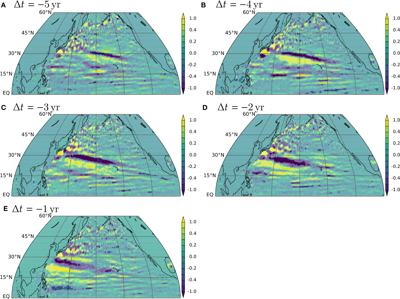
Figure 10 Lead-lag regression ${\alpha }_{\Delta t}(x,y)\tilde{q}(t,m)$ between $\tilde{q}$ and $\tilde{\psi }$ for $\Delta t=-5,\dots ,-1$ calculated on a 0.5° × 0.5° grid. A negative $\Delta t$ means that $\tilde{\psi }$ leads $\tilde{q}$ (Section 2.2.2). To make these plots compatible with Figure 3, $\alpha$ is multiplied by $\tilde{q}(t=1986,m=1)$, and the units of the contour levels are Sverdrups. Color is faded where statistical significance is below the 99% confidence level (Section 2.2.2). Note that the contour intervals increase beyond $\pm 0.5$ Sv to de-emphasize stronger variability.

FIGURE 11

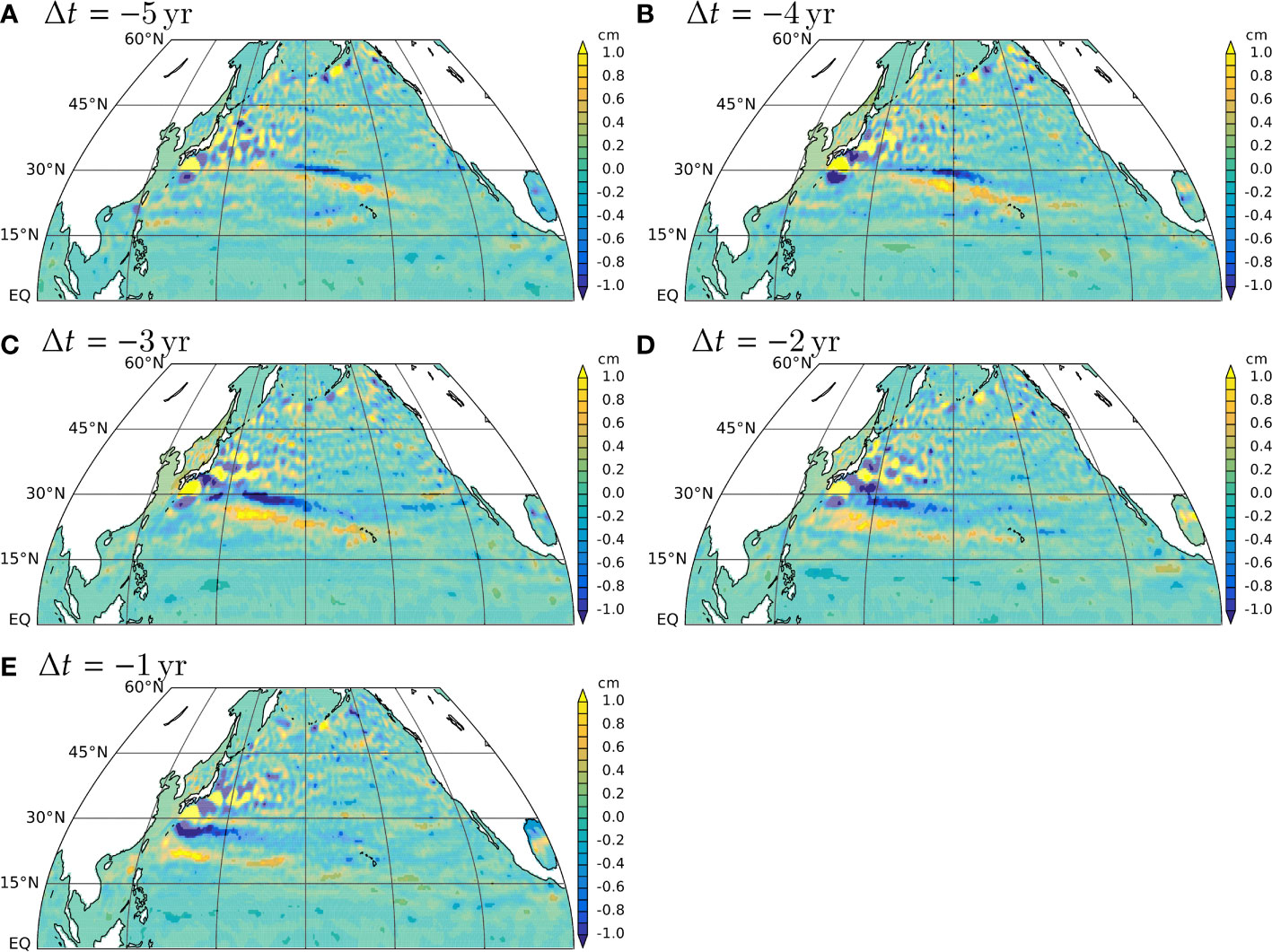
Figure 11 Same as Figure 10 but for sea-surface height. The units of shading are in centimeters.

4.2 Discussion

4.2.1 Zonal jets

The stripes are indeed the most dominant feature in the anomalous barotropic streamfunction itself (not shown) and in its EOFs (not shown either), except for the obvious strong variability in the western boundary currents like the Kuroshio and the Gulf Stream and in the Antarctic Circumpolar Current.

These stripes are a manifestation of “zonal jets” (see the review in the Introduction of Furue et al., 2021 and references cited there). The ocean basins are populated with quasi-barotropic alternating zonal flows. The jets are tilted in the northwest–southeast direction and migrate equatorward and westward (Figures 10, 11). The equatorial migration has also been found in the previous version of OFES (Richards et al., 2006) and in the same OFES2 dataset (Furue et al., 2021) as we use here in the present study. Both the tilt and equatorial migration are consistent with the general westward deepening of the sea floor in the Pacific or the westward thickening of the main pycnocline due to the Subtropical Gyre according to the idealized theoretical studies by Boland et al. (2012) and Khatri and Berloff (2018, 2019).

Does the lagged correlation (Figures 10, 11) mean that these zonal jets force the ensemble anomaly of ITF transport? If so, this variability of ITF is random (that is, not directly determined by external forcing) because the phases of the zonal jets are random (except near the equator) despite the regularity of their propagation (Furue et al., 2021). The stripes in the ensemble anomaly of barotropic streamfunction appear blocked by prominent sea-floor ridges such as Tonga–Kermadec arc and Ninety East Ridge [not shown, but the blockage is visible in the linear regression (Figure 9), clearly for Tonga–Kermadec and barely for Ninety East Ridge], which suggests that the zonal jets are affected by bottom topography. There could then be systematic JEBAR stress that could alter the ITF transport similarly to the way that wind stress in the Pacific determines the overall ITF transport (Godfrey, 1989). According to (Godfrey’s, 1989) island rule, wind stress along latitudes just north of Halmahera and along latitudes just south of the southern tip of Australia (if we ignore the blockage by New Zealand) is key. When particularly large jets arrive north of Halmahera, the ITF transport would increase or decrease, and this anomaly would run across the three ocean basins in the southern hemisphere at a speed of barotropic adjustment (Figure 9). The weakness of the lagged correlation with the southern hemisphere field (Section 3.5.2; Supplementary Figure S5) might be explained by the blockage of the stripes by the Tonga–Kermadec ridge (anonymous reviewer, private communication).

This hypothesis could also explain the apparent weak ∼4-year peak in the autocorrelation (Supplementary Figure S2) through the potential periodicity in the migration of zonal jets. For example, a weak yellow (positive) anomaly is located in southern Japan, and another is located in Taiwan at lag 5 (Figure 10). At lag 4, stronger positive anomalies extend eastward or southeastward from southern Japan and from Taiwan. At lag 1, similar positive anomalies are located at similar latitudes. This suggests a potential periodicity of 3–4 years.

The strong negative simultaneous correlation extending eastward or southeastward from Taiwan in Figure 9 is puzzling. One hypothesis to explain this is that the entire set of positive and negative stripes between Taiwan and Halmahera, which systematically migrates toward the equator, is actually correlated with the ITF transport anomaly. Another hypothesis is that this negative anomaly in Taiwan is related to the magnitude of the transport through the South China Sea to the Indian Ocean. This is an interesting subject for future investigation.

Calil (2023) showed that zonal jets at depth are much more robust in the 1/30°-resolution version of their Atlantic model than in their 1/10°-resolution version. Furue et al. (2021) also found that OFES2’s zonal jets have roughly half the amplitude of the observation by Cravatte et al. (2017) in the central-to-eastern tropical Pacific. If these findings apply to the western tropical and subtropical Pacific and if the zonal jets really have something to do with the intrinsic variability of the ITF transport, the real amplitude of the intrinsic variability might be larger than found in the present study.

In any case, this is speculation, and the evidence we have provided is hardly sufficient. We just propose this hypothesis for future studies to test.

4.2.2 Concluding remarks

Sasaki et al. (2018) found an increase in the ITF transport when a tidal-mixing parameterization is introduced to OFES2. Considering the size of the ensemble spread found in the present study, one might wonder whether the increase they found may have been just an ensemble spread triggered by the introduction of tidal mixing. The increase, however, is a long-term trend from 1960 to 2014 (their Figure 1) and therefore is not likely a stochastic (random) variability, as the latter is not persistent in time (Figure 2B). The interannual variability they found, on the other hand, should include the variability we have found in the present study.

Intrinsic variability should depend on resolution, model parameters, forcing, and boundary conditions. Since chaoticness depends on nonlinearity, coarser models are expected to be generally less chaotic. Damping of variability would naturally weaken intrinsic variability, and therefore surface heat flux would dampen it and mixing would, too. The so-called "mixed boundary conditions" are, however, known to produce chaotic oscillation in coarse-resolution models with large vertical diffusion (Huang and Chou, 1994).

Finally, the present study has explored mainly barotropic circulation. The vertical structure, however, has a number of curious features, as shown in Sections 3.3.2 and 3.3.3. Since the speed of horizontal propagation of baroclinic waves strongly depends on their vertical structure, much more sophisticated analyses would be necessary than those employed in the present study. The vertical structure of the ITF’s intrinsic variability will be an interesting subject of future studies.

Data availability statement

We will provide the dataset on reasonable requests from interested researchers. Requests to access these datasets should be directed to https://www.jamstec.go.jp/ofes/, https://doi.org/10.17596/0002029, ryofurue@gmail.com.

Author contributions

RF conceived the study, carried out the analyses, and wrote the manuscript. MN discussed the analyses and edited the manuscript. HS prepared and processed the OGCM data and participated in the discussion of the analyses. All authors contributed to the article and approved the submitted version.

Acknowledgments

M. Feng provided the original monthly dataset of ITF transport estimates behind Figure 5 of Feng et al. (2018). From this data file, we calculated annual averages (Section 3.1). The discussions with Pavel Berloff, Takeshi Doi, and Ingo Richter (in alphabetical order) have been helpful. Comments from reviewers have helped substantially improve the manuscript. The OFES2 integration was conducted on the Earth Simulator with the support of JAMSTEC. We wish to acknowledge the use of the PyFerret program for analysis and graphics in this paper. PyFerret is a product of NOAA’s Pacific Marine Environmental Laboratory. (Information is available at http://ferret.pmel.noaa.gov/Ferret/).

Conflict of interest

The authors declare that the research was conducted in the absence of any commercial or financial relationships that could be construed as a potential conflict of interest.

Publisher’s note

All claims expressed in this article are solely those of the authors and do not necessarily represent those of their affiliated organizations, or those of the publisher, the editors and the reviewers. Any product that may be evaluated in this article, or claim that may be made by its manufacturer, is not guaranteed or endorsed by the publisher.

Supplementary material

The Supplementary Material for this article can be found online at: https://www.frontiersin.org/articles/10.3389/fmars.2023.1117304/full#supplementary-material

References

Boland E. J. D., Thompson A. F., Shuckburgh E., Haynes P. H. (2012). The formation of nonzonal jets over sloped topography. J. Phys. Oceanogr. 42 (10), 1635–1651. doi: 10.1175/JPO-D-11-0152.1

CrossRef Full Text | Google Scholar

Calil P. H. R. (2022). High-resolution, basin-scale simulations reveal the impact of intermediate zonal jets on the Atlantic oxygen minimum zones. J. Adv. Model. Earth Syst. 15, e2022MS003158. doi: 10.1029/2022MS003158

CrossRef Full Text | Google Scholar

Cravatte S., Kestenare E., Marin F., Dutrieux P., Firing E. (2017). Subthermocline and intermediate zonal currents in the tropical Pacific Ocean: paths and vertical structure. J. Phys. Oceanogr. 47 (9), 2305–2324. doi: 10.1175/JPO-D-17-0043.1

CrossRef Full Text | Google Scholar

England M. H., Huang F. (2005). On the interannual variability of the Indonesian Throughflow and its linkage with ENSO. J. Clim. 18 (9), 1435–1444. doi: 10.1175/JCLI3322.1

CrossRef Full Text | Google Scholar

Farmer J. D. (1982). Information dimension and the probabilistic structure of chaos. Z. Naturforsch. A 37 (11), 1304–1326. doi: 10.1515/zna-1982-1117

CrossRef Full Text | Google Scholar

Feng M., Zhang N., Liu Q., Wijffels S. (2018). The Indonesian Throughflow, its variability and centennial change. Geosci. Lett. 5 (1), 3. doi: 10.1186/s40562-018-0102-2

CrossRef Full Text | Google Scholar

Furue R., Nonaka M., Sasaki H. (2021). On the statistics of the zonal jets in the eastern equatorial Pacific and eastern North Pacific in an ensemble of eddy-resolving ocean general circulation model runs. Ocean Modell. 159, 101761. doi: 10.1016/j.ocemod.2021.101761

CrossRef Full Text | Google Scholar

Godfrey J. S. (1989). A Sverdrup model of the depth-integrated flow for the world ocean allowing for island circulations. Geophys. Astrophys. Fluid Dyn. 45, 89–112. doi: 10.1080/03091928908208894

CrossRef Full Text | Google Scholar

Gordon A. L., Sprintall J., Van Aken H. M., Susanto D., Wijffels S., Molcard R., et al. (2010). The Indonesian Throughflow during 2004–2006 as observed by the INSTANT program. Dyn. Atmos. Oceans 50 (2), 115–128. doi: 10.1016/j.dynatmoce.2009.12.002

CrossRef Full Text | Google Scholar

He Z., Feng M., Wang D., Slawinski D. (2015). Contribution of the Karimata Strait transport to the Indonesian Throughflow as seen from a data assimilation model. Cont. Shelf Res. 92, 16–22. doi: 10.1016/j.csr.2014.10.007

CrossRef Full Text | Google Scholar

Huang R. X., Chou R. L. (1994). Parameter sensitivity study of the saline circulation. Clim. Dyn. 9 (8), 391–409. doi: 10.1007/BF00207934

CrossRef Full Text | Google Scholar

Kalnay E. (2002). Atmospheric modeling, data assimilation and predictability (New York: Cambridge University Press). doi: 10.1017/CBO9780511802270

CrossRef Full Text | Google Scholar

Khatri H., Berloff P. (2018). A mechanism for jet drift over topography. J. Fluid Mech. 845, 392–416. doi: 10.1017/jfm.2018.260

CrossRef Full Text | Google Scholar

Khatri H., Berloff P. (2019). Tilted drifting jets over a zonally sloped topography: effects of vanishing eddy viscosity. J. Fluid Mech. 876, 939–961. doi: 10.1018057/jfm.2019.579

CrossRef Full Text | Google Scholar

Komori N., Takahashi K., Komine K., Motoi T., Zhang X., Sagawa G. (2005). Description of sea-ice component of coupled ocean–sea-ice model for the Earth Simulator (OIFES). J. Earth Simulator 4, 31–45. doi: 10.32131/jes.4.31

CrossRef Full Text | Google Scholar

Large W. G., Yeager S. G. (2004). Diurnal to decadal global forcing for ocean and sea-ice models: the data sets and flux climatologies. Technical report. (Boulder, CO: UCAR/NCAR). doi: 10.5065/D6KK98Q6

CrossRef Full Text | Google Scholar

Lima L. N., Pezzi L. P., Penny S. G., Tanajura C. A. S. (2019). An investigation of ocean model uncertainties through ensemble forecast experiments in the Southwest Atlantic ocean. J. Geophys. Res. Oceans 124 (1), 432–452. doi: 10.1029/2018JC013919

CrossRef Full Text | Google Scholar

Liu Q. Y., Feng M., Wang D., Wijffels S. (2015). Interannual variability of the Indonesian Throughflow transport: a revisit based on 30 year expendable bathythermograph data. J. Geophys. Res. Oceans 120 (12), 8270–8282. doi: 10.1002/2015JC011351

CrossRef Full Text | Google Scholar

Locarnini R. A., Mishonov A. V., Antonov J. I., Boyer T. P., Garcia H. E., Baranova O. K., et al. (2013). World Ocean Atlas 2013, volume 1: temperature. Ed. Levitus S. (NOAA Atlas NESDIS), 73. Available at: https://www.nodc.noaa.gov/OC5/woa13/pubwoa13.html.

Google Scholar

McCreary J. P., Miyama T., Furue R., Jensen T., Kang H. W., Bang B., et al. (2007). Interactions between the Indonesian Throughflow and circulations in the Indian and Pacific Oceans. Prog. Oceanog. 75, 70–114. doi: 10.1016/j.pocean.2007.05.004

CrossRef Full Text | Google Scholar

Nonaka M., Sasai Y., Sasaki H., Taguchi B. (2016). How potentially predictable are midlatitude ocean currents? Sci. Rep. 6, 20153. doi: 10.1038/srep20153

PubMed Abstract | CrossRef Full Text | Google Scholar

Nonaka M., Sasaki H., Taguchi B., Schneider N. (2020). Atmospheric-driven and intrinsic interannual-to-decadal variability in the Kuroshio Extension Jet and eddy activities. Front. Mar. Sci. 7. doi: 10.3389/fmars.2020.547442

CrossRef Full Text | Google Scholar

North G. R., Bell T. L., Cahalan R. F., Moeng F. J. (1982). Sampling errors in the estimation of empirical orthogonal functions. Mon. Weather Rev. 110 (7), 699–706. doi: 10.1175/1520-0493(1982)110<0699:SEITEO>2.0.CO;2

CrossRef Full Text | Google Scholar

Pacanowski R. C., Griffies S. M. (2000). MOM 3.0 manual. Technical report. (Princeton, NJ: Geophys. Fluid Dyn. Lab., NOAA). Available at: https://www.gfdl.noaa.gov/ocean-model/.

Google Scholar

Potemra J. T., Hautala S. L., Sprintall J. (2003). Vertical structure of Indonesian Throughflow in a large-scale model. Deep Sea Res. 50 (12), 2143–2161. doi: 10.1016/S0967-0645(03)00050-X

CrossRef Full Text | Google Scholar

Richards K. J., Maximenko N. A., Bryan F. O., Sasaki H. (2006). Zonal jets in the Pacific Ocean. Geophys. Res. Lett. 33, L03605. doi: 10.1029/2005GL024645

CrossRef Full Text | Google Scholar

Sasaki H., Kida S., Furue R., Aiki H., Komori N., Masumoto Y., et al. (2020). A global eddying hindcast ocean simulation with OFES2. [The data homepage is https://doi.org/10.17596/0002029.]. Geosci. Model. Dev. 13 (7), 3319–3336. doi: 10.5194/gmd-13-3319-2020

CrossRef Full Text | Google Scholar

Sasaki H., Kida S., Furue R., Nonaka M., Masumoto Y. (2018). An increase of the Indonesian Throughflow by internal tidal mixing in a high-resolution quasi global ocean simulation. Geophys. Res. Lett. 45 (16), 8416–8424. doi: 10.1029/2018GL078040

CrossRef Full Text | Google Scholar

Sen Gupta A., McGregor S., van Sebille E., Ganachaud A., Brown J. N., Santoso A. (2016). Future changes to the Indonesian Throughflow and Pacific circulation: the differing role of wind and deep circulation changes. Geophys. Res. Lett. 43 (4), 1669–1678. doi: 10.1002/2016GL067757

CrossRef Full Text | Google Scholar

Shukla J. (1998). Predictability in the midst of chaos: a scientific basis for climate forecasting. Science 282 (5389), 728–731. doi: 10.1126/science.282.5389.728

PubMed Abstract | CrossRef Full Text | Google Scholar

Tsujino H., Urakawa S., Nakano H., Small R. J., Kim W. M., Yeager S. G., et al. (2018). JRA-55 based surface dataset for driving ocean–sea-ice models (JRA55-do). Ocean Modell. 130, 79–139. doi: 10.1016/j.ocemod.2018.07.002

CrossRef Full Text | Google Scholar

Wajsowicz R. C. (1993). The circulation of the depth-integrated flow around an island with application to the Indonesian Throughflow. J. Phys. Oceanogr. 23 (7), 1470–1484. doi: 10.1175/1520-0485(1993)023<1470:TCOTDI>2.0.CO;2

CrossRef Full Text | Google Scholar

Walker H. M. (1940). Degrees of freedom. J. Educ. Psychol. (US) 31, 253–269. doi: 10.1037/h0054588

CrossRef Full Text | Google Scholar

Wilks D. S. (2011). “Chapter 12 - principal component (EOF) analysis,” in Statistical methods in the atmospheric sciences. International Geophysics, vol. 100. Ed. Wilks D. S. (Oxford: Academic Press), 519–562. doi: 10.1016/B978-0-12-385022-5.00012-9

CrossRef Full Text | Google Scholar

Zweng M. M., Reagan J. R., Antonov J. I., Locarnini R. A., Mishonov A. V., Boyer T. P., et al. (2013). World Ocean Atlas 2013, volume 2: salinity. Ed. Levitus S. (NOAA Atlas NESDIS), 74. Available at: https://www.nodc.noaa.gov/OC5/woa13/pubwoa13.html.

Google Scholar

A. Appendix

This appendix provides details of Sections 2.2.2 and 2.2.3. In this appendix, we omit the tilde symbol so that γ and q denote ensemble anomalies [definition (1)]. For convenience, we define a norm (length) of a variable γ(j,l,m) as

$$\parallel \gamma \parallel (j)\equiv {[{\displaystyle {\sum }_{l,m}}{\gamma }^2(j,l,m)]}^{1/2},$$

which is a function of $j$.

A.1. Linear regression

We denote the ensemble anomaly of the ITF transport by $q(l,m)$ and we find a component of $\gamma$ which is maximally correlated with $q$. In other words, we separate $q$ into two components, one is perfectly correlated with $q$ and the other uncorrelated:

$\begin{array}{ll}\gamma (j,l,m)=\alpha (j)q(l,m)+{\gamma }^{″}(j,l,m).& \text{(A1)}\end{array}$

This $\alpha$ is often called the linear regression coefficient. This method can be viewed as a simple modeling: $\gamma \approx \alpha q$ or $q\approx {\alpha }^{-1}\gamma$. From the data $\gamma (j,l,m)$, $\alpha (j)$ can be uniquely determined at each gridpoint $j$ using the standard least-squares fitting.

It can be shown that $\alpha (j)={\displaystyle {\sum }_{l,m}}\gamma (j,l,m)q(l,m)/\Vert q{\Vert }^2$ and that the correlation coefficient between $\gamma$ and $q$ is $r(j)=\alpha (j)\parallel q\parallel /\parallel \gamma \parallel .$ In this sense, α can be regarded as representing correlation between γ and q. It can also be shown that the other component, ${\gamma }^{″}$, is uncorrelated with $q(l,m)$, that is, ${\displaystyle {\sum }_{l,m}}{\gamma }^{″}(j,l,m)q(l,m)=0$. The regression coefficient does not depend on $l$ or $m$ and represents the spatial pattern of the correlation; and $\alpha (j)q(l,m)$ is the spatial distribution of this component of $\gamma$ at $(l,m)$ as indicated by (A1).

A lead-lag regression can be similarly defined by

$$\gamma (j,l+\text{Δ}t,m)={\alpha }_{\text{Δ}t}(j)q(l,m)+{\gamma }^{″}(j,l+\text{Δ}t,m).$$

We use the symbol $\text{Δ}t$ just for convenience in explaining the results in Section 3 but it is actually an integer and can also be written as $\text{Δ}l$. Note that $1-\text{Δ}t\le l\le L$ when $\text{Δ}t\le 0$ or $1\le l\le L-\text{Δ}t$ when $\text{Δ}t\ge 0$. The number of time steps used for the calculation, therefore, is reduced from $L$ to $L-\left|\text{Δ}t\right|$. When $\text{Δ}t<0$, the regression coefficient represents the linear relation between the past $\gamma (l-\left|\text{Δ}t\right|)$ and the present $q(l)$.

Statistical significance. Even if γ varies purely randomly, the correlation coefficient between the observed $\gamma$ and $q$ can still be non-zero by chance. To test whether $\gamma$ and $q$ are really correlated, we use the standard t-test: assuming that $\gamma$ is purely random, we calculate for the given $q$ the probability that a particular value of $\alpha$ is larger than $a$ and find a value of $a$ such that the probability that $\alpha >a$ is 1% and the probability that $\alpha <-a$ is 1% and then regard values of $\mathrm{|\alpha |}$ that is larger than $a$ as significant. Note that the value of the threshold $a$ depends on $j$ because it depends on ∥$q$∥ and ∥$\gamma$∥.

A.2. Ensemble–temporal EOFs

If $\gamma$ is the vertical distribution of a variable, its variance may be defined as

$\begin{array}{ll}{\displaystyle {\int }_{z_2}^{z_1}dz{[\gamma (z)]}^2={\sum }_{k=1}^N\text{Δ}{z}_k{\gamma }_k^2={\mathbf{\gamma }}^{T}W\mathbf{\gamma },}& \text{(A2)}\end{array}$

where $\text{Δ}{z}_k$ is the thickness of layer $k$, $W=\text{diag }(\text{Δ}{z}_1,\dots ,\text{Δ}{z}_N)$, and γ is the column vector of $[{\gamma }_1,\dots ,{\gamma }_N]$. For generality, we write $W\equiv \text{diag }(w_1,\dots ,w_N)$ below.

A.2.1. Calculation of weighted EOFs

As in the discussion in the previous subsection, we denote the value of $\gamma$ at $(l,m)$ and at gridpoint $j$ as $\gamma (j,l,m)$ and we consider EOFs for the $N\times N$, weighted covariance matrix (North et al., 1982)

$${\left[{\displaystyle \sum }_{l,m}\sqrt{w_j}\gamma (j,l,m)\gamma (j^{\prime },l,m)\sqrt{w_{j^{\prime }}}\right]}_{j=1,\dots ,N;{\mathrm{ j}}^{\prime }=1,\dots ,N}.$$

The eigenvectors of this matrix form an orthogonal basis and we also normalize them so that they form an orthonormal basis in the sense that

$${\mathit{f}}_n^T{\mathit{f}}_{n^{\prime }}={\delta }_{n,n^{\prime }}.$$

These are the usual EOFs, but the more natural EOF modes are ${\mathit{e}}_n\equiv W^{-1/2}{\mathit{f}}_n$. It immediately follows from the orthonormality relation of $\mathit{f}$ that

$\begin{array}{ll}{\mathit{e}}_n^{T}W{\mathit{e}}_{n^{\prime }}={\delta }_{n,n^{\prime }}.& \text{(A3)}\end{array}$

This relation corresponds to

$${\displaystyle {\int }_{z_2}^{z_1}}\text{ d}z{e}_n(z)e_{n^{\prime }}(z)={\delta }_{n,n^{\prime }}$$

as above. These EOFs are thus orthonormal with respect to their natural integration.

A.2.2. Expansion into EOFs.

The spatial distribution of the variable

$$\mathit{\gamma }(l,m)=\left[\begin{array}{c}{\gamma }_{1,l,m}\\ ⋮\\ {\gamma }_{N,l,m}\end{array}\right]$$

at each timestep l and for each member m can be expanded into the EOF modes $\left\{{\mathit{e}}_1,\dots ,{\mathit{e}}_N\right\}$, as they form a basis of the $N$-dimensional space, as

$\begin{array}{ll}\mathit{\gamma }(l,m)={\displaystyle \sum _n}{\varphi }_n(l,m){\mathit{e}}_n.& \text{(A4)}\end{array}$

In other words, the spatial distribution of $\gamma$ at each $(l,m)$ is expressed as a superposition of the EOFs ($\mathit{e}$’s), and then $\varphi$’s are the amplitudes, at each $(l,m)$, of the EOFs. The expansion coefficients $\varphi$, after normalization, are often called "principal components" in the oceanographic, meteorological, and climate-science community (e.g., Wilks 2011).

It can then be shown from (A4) that

$${\mathit{\gamma }}^{T}W\mathit{\gamma }={\displaystyle \sum _n}{\varphi }_n^2(l,m),$$

using the orthonormality relation between $\mathit{e}$’s, which is formula (A3). It follows form (A2) that

$\begin{array}{ll}{\displaystyle {\int }_{z_2}^{z_1}}\text{d}z{[\gamma (z;l,m)]}^2={\displaystyle \sum _n}{\varphi }_n^2(l,m)& \text{(A5a)}\end{array}$

(North et al. 1982), which states that mode n contributes to the total variance by ${\varphi }_n^2$ at each $(l,m)$. The contribution of EOF mode $n$ is naturally ${\varphi }_n^2/({\displaystyle {\sum }_n{\varphi }_n^2})$ at each $(l,m)$. The overall variance is then

$\begin{array}{ll}{\displaystyle \sum _{l,m}}{\displaystyle {\int }_{z_2}^{z_1}}\text{d}z{[\gamma (z;l,m)]}^2={\displaystyle \sum _n}\left[{\displaystyle \sum _{l,m}}{\varphi }_n^2(l,m)\right]\equiv {\displaystyle \sum _n}{\lambda }_n& \text{(A5b)}\end{array}$

Therefore, ${\lambda }_n={\displaystyle {\sum }_{l,m}}{\varphi }_n^2(l,m)$ represents the overall contribution of mode n to the overall total. (As is well known, λn can be shown to be equal to the eigenvalue, corresponding to eigenvector f_n, of the covariance matrix. See, e.g., Wilks 2011.)

Note that we customarily order the EOFs in the order of decreasing ${\lambda }_n$. At each $(l,m)$, however, the contributions of the modes, (A5a), generally are in a different order. For example, at $t=1986$ and $m=1$, EOF3 has the largest contribution followed by EOF2 (Figure 6, lower-left panel).

The conservation of variance (A5a) and (A5b) naturally follows from the weighting, $W$. Without the weights of $\text{Δ}z$, moreover, near-surface variability would get disproportionate weights in the calculation of EOFs. Another way to solve these problems is to map the original variable onto a uniform grid. If it is mapped onto a coarse uniform grid, near-surface variabilities may be lost, and so it has to be mapped onto a fine grid as to resolve the surface variability. Moreover, uniform gridding is not possible for a latitude–longitude distribution such as sea-surface temperature.