 Sheila N. Estrada-Allis1*
 Ángel Rodríguez-Santana2
 Alberto C. Naveira-Garabato3,4
 Luis García-Weil2Mireya Arcos-Pulido2
 Mikhail Emelianov4
- 1Department of Physical Oceanography, Ensenada Center for Scientific Research and Higher Education (CICESE), Ensenada, Baja California, Mexico
- 2Departamento de Física, Facultad de Ciencias del Mar, Universidad de Las Palmas de Gran Canaria (ULPGC), Las Palmas de Gran Canaria, Spain
- 3National Oceanography Centre, University of Southampton, Southampton, United Kingdom
- 4Physical and Technological Oceanography, Instituto de Ciencias del Mar (CSIC), Barcelona, Spain
The filaments of the African Eastern Boundary Upwelling System (EBUS) are responsible for feeding nutrients to the oligotrophic waters of the northeastern Atlantic. However, turbulent mixing associated with nutrient uplift in filaments is poorly documented and has been mainly evaluated numerically. Using microstructure profiler measurements, we detected enhanced turbulent kinetic energy dissipation rates (ε) within the Cape Ghir upwelling filament. In contrast to previous studies, this enhancement was not related to symmetrical instabilities induced by down-front winds but to an increase in vertical current shear at the base of the mixed layer (). In order to quantify the impact of vertical shear and the influence of the active mixing layer depth () in the filament, a simple one-dimensional (1D) turbulent entrainment approach was used. We found that the effect of turbulent enhancement, together with the isopycnal morphology of the filament front, drove the formation of local positive entrainment zones (), as was deeper than . This provided suitable conditions for the entrainment of cold, nutrient-rich waters from below the filament pycnocline and the upward transport of biophysical properties to the upper boundary layer of the front. We also found that diapycnal nutrient fluxes in stations influenced by the filament (1.35 mmol m-2 d-1) were two orders of magnitude higher than those of stations not affected by the filament front (0.02 mmol m-2 d-1). Despite their importance, the effects of vertical shear and have often been neglected in entrainment parameterizations. Thus, a modified entrainment parameterization was adapted to include vertical shear and observed ε, which are overestimated by existing parameterizations. To account for the possible role of internal waves in the generation of vertical shear, we considered internal wave scaling to parameterize the observed dissipation. Using this adapted parameterization, the average entrainment velocities were six times (6 m d-1) higher than those obtained with the classic parameterization (1 m d-1).
1 Introduction
Phytoplankton productivity is limited by nutrient availability, especially in oligotrophic areas such as subtropical gyres. In Eastern Boundary Upwelling Systems (EBUS), filaments are examples of frontal systems that are able to supply nutrients from below the pycnocline to the upper boundary layer of the ocean. Moreover, cold and nutrient-rich water that is upwelled along the coast can be transported offshore by filaments, which are typically narrow (10 km) and elongated (100 km) structures with vertical extensions of ~100 m. These structures are often located near coastline irregularities (Hagen et al., 1996; Sangrà et al., 2015) and identifiable by low surface temperatures and high chlorophyll-a concentrations (Sangrà et al., 2015).
The pycnocline usually outcrops within filaments, producing sharp differences in the upper layer of the ocean with respect to the characteristics of the surrounding waters, which are generally well-mixed (Dewey and Moum, 1990; Pelegrí et al., 2005b; Arcos-Pulido et al., 2014). These thermohaline fronts affect the lateral buoyancy gradient, thus providing suitable conditions for diapycnal mixing through mechanisms such as vertical shear. Diapycnal mixing associated with submesoscale frontal systems is particularly important given that it involves the exchange of surface heat, buoyancy fluxes, and the vertical transport of tracers, such as nutrients, from below the pycnocline to surface waters (e.g., Hales et al., 2005; Li et al., 2012; Arcos-Pulido et al., 2014).
Despite the importance of these ubiquitous structures, few studies have analyzed how turbulence may be enhanced within filaments using turbulent kinetic energy (TKE) dissipation rates () obtained with direct microstructure measurements. Dewey et al. (1993) observed elevated subsurface , which they attributed to mean shear turbulence generated within submesoscale structures known as minifilaments. Other observations of microstructures have suggested that surface-induced mixing may be enhanced by the proximity of filament fronts, resulting in strong horizontal density gradients that can help maintain the frontal system (Dewey and Moum, 1990). Other authors have suggested that two-dimensional turbulence is generated by symmetrical instabilities due to the low potential vorticity of down-front winds and/or atmospheric buoyancy loss (e.g., D’Asaro et al., 2011; Thomas et al., 2013; Peng et al., 2020). Collectively, these studies demonstrate that turbulence in the upper boundary layer may be notably enhanced within filaments; however, the mechanisms responsible for this enhanced turbulence remain unclear.
From a one-dimensional (1D) point of view, there are three primary TKE sources that control turbulence in the upper boundary layer (Niiler and Kraus, 1977): (i) wind stirring, (ii) convection forces, and (iii) vertical shear due to horizontal currents at the base of the mixed layer. These three sources are balanced by the dissipation term, which represents the main TKE sink. In order to close the system of equations of the 1D TKE budget, the entrainment rate () must be considered, which is a temporal rate of change of themixed layer depth (e.g., Niiler and Kraus, 1977; Cronin and McPhaden, 1997; Wade et al., 2011) that describes the turbulent and diapycnal velocity acting at the base of the mixed layer. Turbulent entrainment increases , decreases temperature, and transports hydro-physical properties, such as heat, salinity, and nutrients, between the upper and lower ocean layers. This is particularly important in upwelling regions given that entrainment helps to upwell nutrient-rich waters from below the pycnocline to the nutrient-poor upper layers. Thus, entrainment can be viewed as a proxy of TKE sources and sinks that control turbulence from the pycnocline through the upper boundary layer.
The parameterization of entrainment through a 1D TKE budget has been widely used in many bulk mixed layer models (e.g., Deardorff, 1983; Gaspar, 1988; Jacob and Shay, 2003; Nagai et al., 2005; Samson et al., 2009; Liu et al., 2012; Giordani et al., 2013). However, the study of entrainment is itself challenging because its contributions are often overwhelmed by large-scale motions. In recent decades, considerable efforts have been made to elucidate entrainment behavior through laboratory experiments (e.g., Khanta et al., 1977; Deardorff, 1983; Fernando, 1991; Pelegrí and Richman, 1993; Jackson and Rehmann, 2014), modeling setups (e.g., Jacob and Shay, 2003; Sun and Wang, 2008) and observational studies (e.g., Dewey and Moum, 1990; Anis and Moum, 1994; Nagai et al., 2005). However, discrepancies in values are apparent when comparing different entrainment parameterizations (Deardorff, 1983; Anis and Moum, 1994; Jacob and Shay, 2003).
Only a few studies have focused on the characterization of vertical turbulent entrainment in upwelling filament systems, and these have produced contradictory results. Dewey and Moum (1990) showed that wind-induced turbulent entrainment is less efficient in the warm sides of filaments than in their cold sides, where the pycnocline outcrops near the surface. These authors also suggested that entrainment could act to maintain a cool surface signature in upwelling filaments. In another study, Dewey et al. (1993) argued that diapycnal turbulent processes associated with minifilaments are less important than local upwelling or frontogenesis mechanisms. However, it is likely that both processes are related (Estrada-Allis et al., 2019). Indeed, the temporal evolution of vertical velocity suggests that vertical mixing can modulate the magnitude of the ageostrophic term, with elevated near-surface mixing enhancing the vertical velocity.
In another study, Grodsky et al. (2008) used satellite observations of equatorial Atlantic upwelling to demonstrate that thermocline shoaling associated with elevated wind strength increases the entrainment of cold, nutrient-rich water to the mixed layer, leading to phytoplankton blooms. Using a regional model, Giordani et al. (2013) found that entrainment does not contribute to the development of the Atlantic cold tongue. Although these studies have notably improved our understanding of entrainment, the sources that control the TKE balance in the upper boundary layer and consequently turbulent entrainment remain poorly understood.
In this study, we refer to the upper boundary layer as the region comprising both the mixed layer depth () and mixing layer depth (). The latter is the depth at which active mixing processes operate (Brainerd and Gregg, 1995). Some studies have indicated that may play an important role in highly dynamic areas like frontal systems. This is relevant because the vertical transport of heat, momentum, and hydrophysical material within the upper boundary layer is controlled by turbulent mixing (Brainerd and Gregg, 1995; Cisewski et al., 2008; Inoue et al., 2010; Sutherland et al., 2014), with important and consequences for phytoplankton blooms (Franks, 2014).
This study focuses on the filament generated near Cape Ghir, which forms part of the African EBUS (e.g., Hagen, 2001). This recurrent filament is one of the major filaments of the Canary Current Upwelling System (Hagen et al., 1996; Pelegrí et al., 2005a; Pelegrí et al., 2005b) and is able to transport biogeochemical properties offshore more effectively than wind-driven Ekman transport (Álvarez Salgado et al., 2007). Moreover, the Cape Ghir filament is involved in both onshore and offshore export export (Santana-Falcón et al., 2020) and is responsible for up to 63% of the total annual primary production attributed to coastal upwelling (e.g., García-Muñoz et al., 2005). The long-lived (>3 months) westward-propagating mesoscale eddies generated in the Eddy Canary Corridor (Sangrà et al., 2009) can interact with the Cape Ghir filament, exporting nutrients and carbon to the oligotrophic interior regions of the northeastern Atlantic.
The generation of the Cape Ghir filament can be explained by the combined effects of baroclinic instability from the filament jet, seafloor topography, and wind near the cape, which act to deflect the filament offshore (Hagen, 2001; Pelegrí et al., 2005b; Troupin et al., 2012). Due to the enhancement of turbulent mixing within filaments, our primary objective was to investigate the primary TKE sources and sinks within and outside of the Cape Ghir upwelling filament in the upper ocean through an analysis of the bulk 1D TKE balance. Using novel observations of for this region, we analyzed where turbulent mixing takes place and how it relates to the three primary sources of turbulence at the surface by means of an entrainment parameterization. We also evaluated the importance of diapycnal nutrient fluxes at the base of the mixed layer and focused on vertical shear and dissipation as important TKE sources and sinks, respectively. These analyses were conducted using meteorological, hydrographic, and satellite data and microstructure turbulent profiles.
In this study, we show that actual turbulent entrainment parameterizations could be underestimating entrainment rates in highly dynamic areas dominated by mesoscale structures. These low diapycnal velocities will lead to an underestimation of the vertical transport of nutrients and physical properties from the base of the mixed layer to the upper boundary layer of Cape Ghir filament and other similar filaments associated with EBUS.
2 Materials and methods
2.1 Observational data
The hydrographic data used in this study were obtained from a survey of the Cape Ghir region in northwestern Africa, which formed part of the project “Mixing Processes in the Canary Basin (PROMECA)” (Figure 1). The survey was conducted aboard the R/V García del Cid in early fall (18–29 October 2010) when the Trade Winds typically weaken. Conductivity-temperature-depth (CTD), expendable bathythermograph (XBT), and microstructure data were collected at stations located approximately 10 km apart from one another along three transects (A, B, and C in Figure 1).
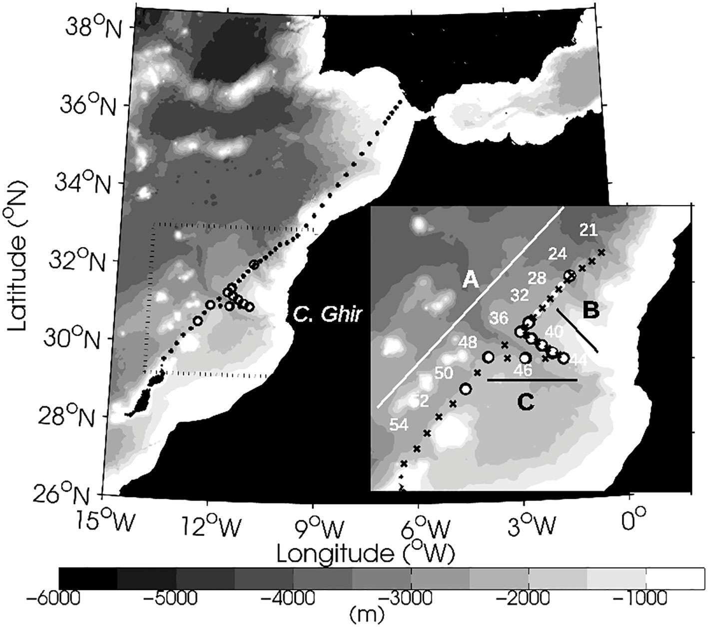
Figure 1 Bathymetry (500 m contour) of the Cape Ghir region and hydrographic sampling stations located around the upwelling filament during October 2010. The region delimited by the black dashed lines encompasses the hydrographic stations surveyed in this study and is shown in greater detail in the inset at the bottom right corner of the figure. Black squares indicate conductivity-temperature-depth (CTD) and Acoustic Doppler Current Profiler (ADCP) stations. White dots indicate microstructure stations. Black dots indicate expendable bathythermograph (XBT) stations. The station numbers appear next to each station, and the transects (A–C) are shown as solid lines.
Wind speed, instantaneous wind speed, wind direction, air temperature, water temperature, relative humidity, air pressure, and incoming solar radiation were recorded at ~2-min intervals by a meteorological station installed onboard the ship. To remain consistent with hydrographic station measurements, the meteorological data were averaged over 2-h intervals (i.e., the time resolution of the CTD profiles).
During the cruise, current velocity data were also collected nearly continuously with a vessel-mounted 75 KHz Ocean Surveyor Acoustic Doppler Current Profiler (SADCP; Teledyne Technologies, Thousand Oaks, CA, USA). The data were processed with Common Ocean Data Access System (CODAS) software (Firing et al., 1995) to obtain vertical bin sizes of 10 m averaged over 2-h periods. An SBE911 plus CTD (Sea-Bird Scientific, Bellevue, WA, USA) was used to produce temperature, salinity, and density profiles (1 dbar vertical resolution). Between each CTD station, vertical temperature profiles were also obtained with XBT Sippican T5 probes (Lockheed Martin, Bethesda, MD, USA) that transmitted to 2000 m depth. The temperature profiles obtained with the XBT probes were smoothed using a classic, low-pass Butterworth filter. A comparison of the CTD and XBT temperature profiles revealed a discrepancy of approximately 10 m. Although uncommon, this offset has been observed in similar studies of the Cape Ghir filament (Pelegrí et al., 2005b). The results of this study are based on CTD rather than XBT vertical profiles.
A TurboMAP-L microstructure profiler Wolk et al. (2002) was used to obtain profiles of . The TurboMAP-L is a vertical free-fall profiler that carries microstructure sensors, including two shear probes and an FP07 thermistor, CTD sensors, and internally mounted accelerometers. The profiler freely falls at a speed of ~0.7 m s-1 while sampling at a rate of 512 Hz. All data were binned at 2-m intervals down to ~470 m depth and processed using TMTools v. 3.04 A.
The location, evolution, and coverage of the Cape Ghir upwelling filament during the survey were determined via sea surface temperature (SST) and chlorophyll-a (Chl) satellite images (Figure 2) obtained from the Moderate Resolution Imaging Spectroradiometer (MODIS) sensors of the AQUA and TERRA satellites. Satellite images were also downloaded from Ocean Color Web (http://oceancolor.gsfc.nasa.gov). Geostrophic surface currents were derived from the sea level anomaly provided by the AVISO altimeter products at a spatial resolution of 1/4° × 1/4°, which were downloaded with OpenDAP from the AVISO Website (http://www.aviso.altimetry.fr/en/home.html).
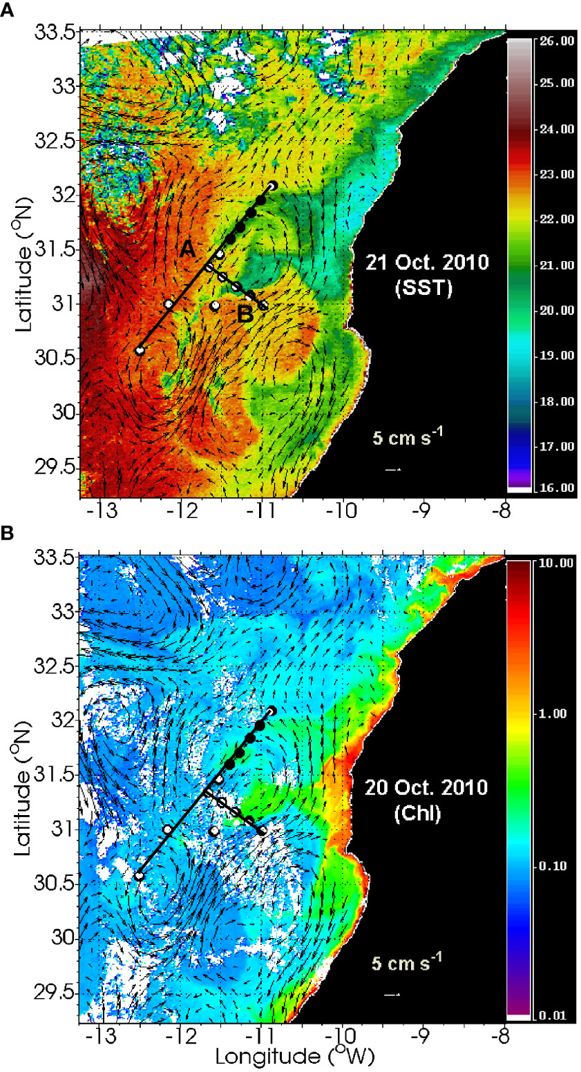
Figure 2 Snapshots of (A) sea surface temperature (SST, °C) from MODIS-Terra for 21 October 2010 at 14:25 h and (B) chlorophyll-a (Chl, mg m-3) from MODIS-Aqua for 20 October 2010 at 13:45 h. Superimposed vectors denote the magnitude and direction of the geostrophic velocity field for the same days derived with AVISO Sea Level Anomaly data (1/4°horizontal resolution). Both transect A and B are shown as solid black lines. Black dots indicate conductivity-temperature-depth (CTD) and Acoustic Doppler Current Profiler (ADCP) stations. The white dots indicate microstructure stations.
2.2 Microstructure data processing
To obtain , we first removed spikes from the turbulence profiles to obtain the shear fluctuation power spectrum, , from the fall speed of the profiler, where k is the wavenumber determined from its fall speed. Assuming isotropic turbulence Hinze, 1979, observed was estimated by integrating within an appropriate wavenumber range following the methods of Oakey (1982):
where v is the molecular viscosity coefficient with a value of 1 × 10⁻⁶ m2s-1 and is the lowest cutoff wavenumber, which was set to 1 cpm given the physical scale of the microstructure shear probe. In contrast, the upper limit of integration, , is the highest vertical wavenumber free of noise and is usually taken to be the Kolmogorov wavenumber . After segmenting each microstructure profile within vertical bin sizes of 2 m, the observed shear spectrum was fitted to the Nasmyth empirical universal spectra for turbulence (Oakey, 1982; Wolk et al., 2002). This spectrum is considered to be representative of the spectral form of oceanic turbulence and is commonly used to verify shear spectrum measurements. An example of micro-shear power spectral density and Nasmyth spectra can be seen in Figure 3 for a depth range of 43 to 45 m at station 24. Given that records of micro-scale velocity shear can be contaminated by noise (e.g., mechanical vibration of the instrument and the influence of the rope at the surface) until the probe reaches a quasi-constant free-falling velocity, the data within the first 16 m of the water column were removed. In addition, the vertical profiles of can exhibit large variability over short time periods. As such, the casts were repeated at least twice at each station.
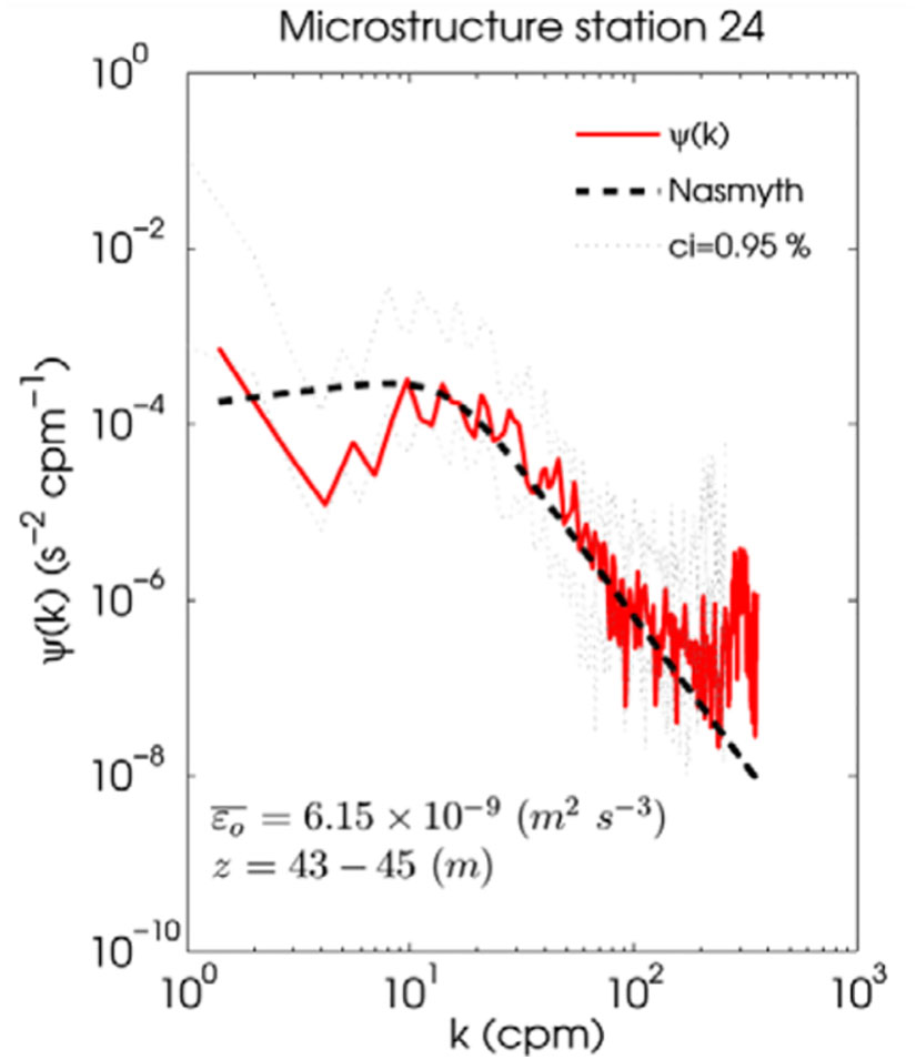
Figure 3 Shear power spectral density, ψ(k) (red solid line), for station 24 from the PROMECA-cruise for a depth range (z) of 43 to 45 m. The Nasmyth universal spectra is shown as a dashed black line. The turbulent kinetic energy (TKE) dissipation rate, , is averaged over the z range. The dotted thin lines indicate the 0.95% confidence interval for the power spectral density calculation. At the bottom, k represents the wavenumber in cycles per minute (cpm).
2.3 Surface fluxes and meteorological-related quantities
To assess the relationship between atmospheric forcing and upper ocean turbulence, meteorological data were used to compute the net surface heat flux () as the sum of four individual components , where is the net shortwave radiation flux, which is the main contributor to during daytime and was directly obtained from the on-board meteorological station. Net longwave radiation () was determined with the equation of Berliand and Berliand (1952):
where is the longwave emissivity from from Dickey et al. (1994), is the Stefan-Boltzman constant, is the air temperature measured at a height of 10 m above the sea surface, is the surface water temperature, is vapor pressure, and is the cloud correction factor with values that range from 0.4 to 1 during daytime, as the sky was mostly clear throughout the study. The sensible heat flux () and latent heat flux () were determined by using the Tropical Ocean Global Atmosphere Coupled Ocean-Atmosphere Response Experiment TOGA-COARE code available in the Matlab Air–Sea toolbox (version 3.0; http://sea-mat.whoi.edu) developed by the air-sea fluxes science group of the TOGA COARE project, which is a version of the bulk flux described in Fairall et al. (1996).
Once the net surface heat fluxes were obtained, we computed the net surface buoyancy flux () as:
where g is acceleration due to gravity, is the specific heat capacity of seawater (), α is the thermal expansion coefficient of seawater ( 2.58 × 10⁻⁴ ± 6.92 × 10⁻⁶°C-1), β is the haline contraction coefficient of seawater (), and is a density reference value (1026 kg m-3). The first term corresponds to the thermal surface buoyancy flux (), and the second term is related to the contribution of the haline surface buoyancy flux (), as suggested by Dorrestein, 1979, where So is surface salinity and (E - P) is the difference between the evaporation and precipitation rates. Surface wind stress () was computed as , where is the reference density of the air 10 m above the sea surface, and is the wind speed. The drag coefficient () was derived from the equation of Large and Pond, 1981 with for and for . Note that only the meteorological-related quantities averaged over a window of 2 h were used for calculations in this study (denoted by superscript s in Figure 4). The window size of 2 h was chosen to include the hour before and the hour after the release of the CTD and reflects the time usually required to complete a CTD cast.
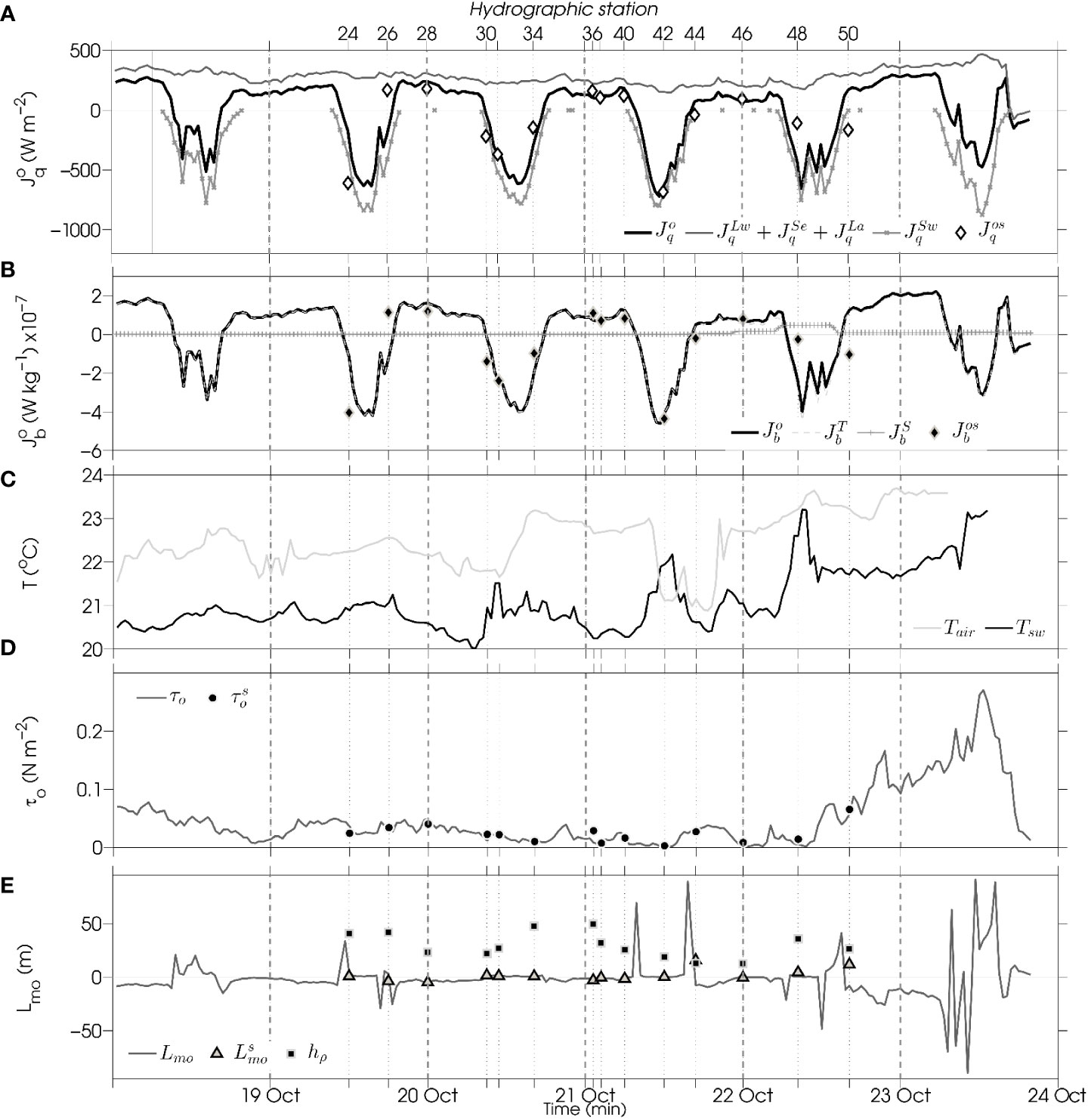
Figure 4 Half-hourly averaged meteorological data. (A) The net surface heat flux (, W m-2, defined positive upward) and the related components of the shortwave radiation flux (), net longwave heat flux (), latent heat flux (), and sensible heat flux (). (B) The net surface buoyancy flux (, W kg-1), defined as the sum of the thermal surface buoyancy flux () and haline surface buoyancy flux (). (C) Sea water temperature (Tsw) and air temperature (Tair, °C). (D) Wind stress (τo, N m-2). (E) Monin-Obukhov length scale (Lmo, m) and mixed layer depth (hρ, m). Symbols superimposed on the time series denoted with a superscript s represent the exact values of each meteorological quantity obtained with the CTD casts from each hydrographic station. The thin vertical dashed lines at the top of the figure indicate the hydrographic stations. The thick dashed lines at the bottom of the figure indicate the end of each day.
2.4 Entrainment parameterization of the 1D TKE budget
Entrainment rates can be parameterized by solving the turbulent closure scheme of the 1D TKE budget (Niiler and Kraus, 1977). Therefore, depending on the sources and sinks that balance the TKE budget of the mixed layer, an assessment of the entrainment parameterization can also help to elucidate which sources of energy drive mixing in the upper boundary layer.
The 1D TKE budget primarily depends on two sinks (i.e., the dissipation term and buoyancy fluxes during daytime) and three sources, namely (i) the production of TKE from mechanical stirring induced by wind stress whose velocity scale is the friction velocity ; (ii) the generation of TKE by buoyancy forces during free-convection in which the velocity scale is the free-convection velocity (Deardorff, 1970); and (iii) TKE produced by shear, which is parameterized via the square of the vertical shear at the base of the mixed layer. In this study, this is represented by the Dynamic Instability Term, , where and represent velocity jumps at the base of the mixed layer calculated as the difference in velocity just below and above the mixed layer depth. All variables and parameters used in this study are summarized in Table 1. It should be noted that other entrainment sources can be included, such as internal waves breaking at the interface (Strang and Fernando, 2001) or Langmuir vortices within the mixed layer (Flór et al., 2010), although further research is required to elucidate the roles of additional sources in entrainment phenomena.
Table 1 List of symbols and parameters that are relevant to the entrainment parameterization.
Several equations have been proposed to compute the entrainment rate as the effective vertical velocity that transports buoyancy across the base of the mixed layer. This study focuses on the parameterization of following the widely used mixed layer bulk model of Gaspar (1988) (, hereinafter), in which the evolution of the mixed layer can be computed as follows:
where m1 = 2.6 and m2 = 1.9 are empirical constants, is the buoyancy jump at the base of the mixed layer calculated as the difference in buoyancy just below and above the mixed layer depth, and is the parameterized TKE dissipation rate. This equation is similar to that of Niiler and Kraus (1977). The main difference between these expressions lies in how is parameterized. Equation (4) does not consider the effect of vertical shear at the base of the mixed layer as a relevant source of TKE. To take into consideration shear-driven turbulence (hereinafter ), we also employed the equation used in the modeling study of Samson et al. (2009):
These authors included the DIT term to evaluate the response of the oceanic mixed layer during a hurricane. In this study, the effect of the DIT term was analyzed under normal wind conditions. In this case, vertical shear will be generated by other sources such as the baroclinicity of the filament front and/or breaking internal waves.
3 Results and discussion
3.1 Hydrographic background of the filament
Upwelling areas are highly dynamic systems (e.g., Barton et al., 1998; Hagen, 2001; Pelegrí et al., 2005b), and studying turbulent processes within these systems is understandably challenging. Unlike in laboratory or modeling experiments, the interactions between processes that operate on different spatiotemporal scales within upwelling systems makes isolating and analyzing a single process quite difficult. In order to describe the physical processes involved in the dynamics of an area, such as within frontal systems, mesoscale eddies, and submesoscale structures, a hydrographical description of the area is required.
The SST and Chl satellite images in Figure 2 show the extension and location of the Cape Ghir upwelling filament over a two-day period (20–21 October 2010). The meander-like structure is identifiable as a cool feature with a high Chl concentration that crosses the sampling stations in transects A and B (Figure 2). The filament waters exhibited a difference of ~2°C from the surrounding waters and were highly conditioned by the mesoscale dynamics of the area, as observed in the superimposed geostrophic currents from the AVISO product in Figure 2. Although representative images with low cloud coverage were chosen as examples, additional images indicated that the filament was present during the sampling period. The filament signal intensified after the last CTD station (i.e., station 50) when stronger wind speeds were recorded. The general description of this filament agrees with those of previous observational studies of African upwelling filaments (e.g., Barton et al., 2001; Hagen, 2001), especially that of Pelegrí et al. (2005b) for the same filament and season in 1995 and 1997.
The vertical sections of salinity (S) and the potential density anomaly () in Figure 5 show doming of isohalines and isopycnals in the northeastern stations of transect A (Figures 5A, B). In addition, the combined vertical CTD-XBT sections also show an elevation of isotherms at the same locations (Figure 6A). This dome-like structure seems to be well correlated with stations that cross the filament front according to satellite imagery (Figure 2).
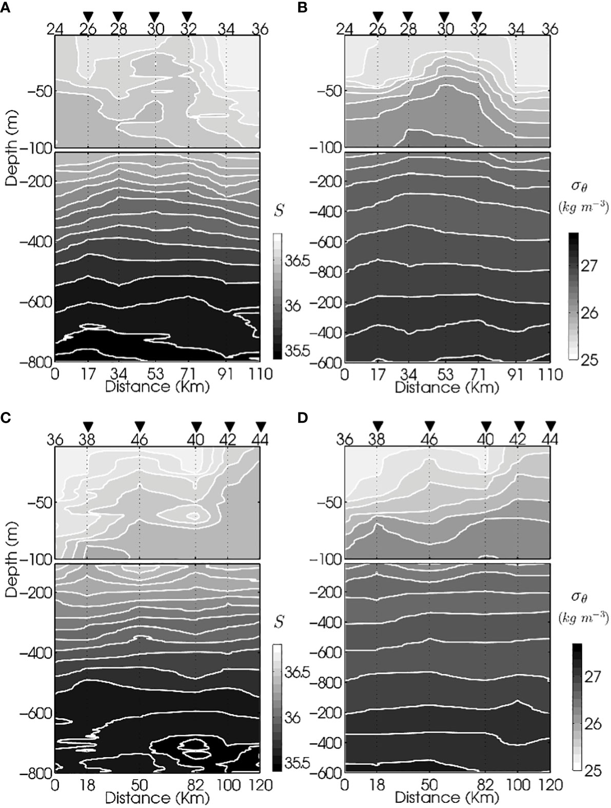
Figure 5 Vertical hydrographic sections derived from CTD profiles of (A) absolute salinity (S) and (B) potential density anomaly (σθ, m kg-3) for transect A and (C) S and (D) σθ for transect B. Contours of S are plotted at 0.5 intervals, while σθ contours are plotted every 0.1 kg m-3. The cumulative distance between stations in km is shown at the bottom of each panel. The hydrographic station numbers are shown at the top of each panel. Inverted triangles indicate stations influenced by the upwelling filament.
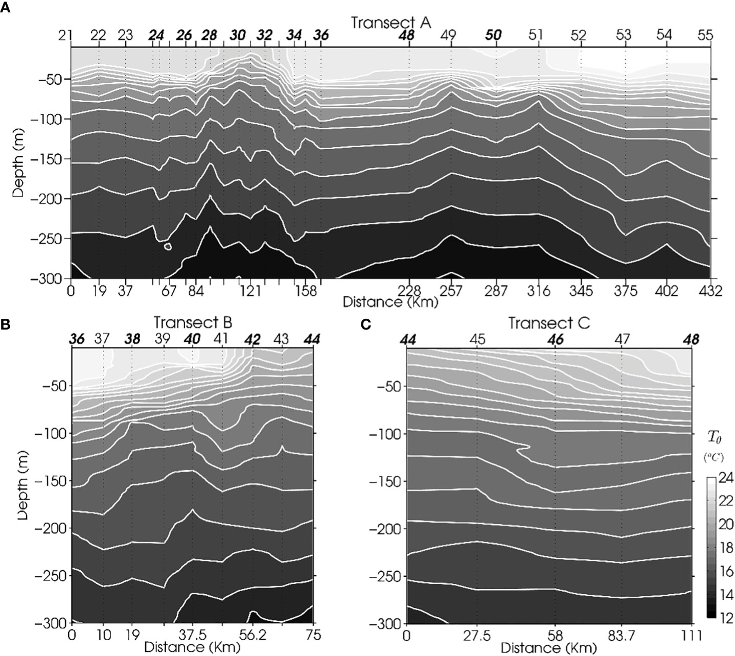
Figure 6 Vertical sections derived from CTD-temperature profiles combined with expendable bathythermograph (XBT) temperature profiles of transects (A) A, (B) B, and (C) C, which was an additional transect. Isotherms are spaced every 0.5°C, and an offset of approximately 10 m was applied to the XBT profiles to ensure consistency with CTD depth. At the top of each panel, numbers in bold italic font denote CTD stations, whereas numbers in Roman font denote XBT stations. Note that not all station numbers are displayed at the top to facilitate viewing. All CTD and XBT stations are taken into account in the vertical sections. The cumulative distance (km) is shown at the bottom of each panel.
Although it was not the aim of this study, it was interesting that the temperature-salinity () relationship (not shown) indicated the presence of a subsurface salinity maximum below the mixed layer (~50 m), with mean values of S = 36.55, Tθ = 19°C, and σθ = [26-26.5] kg m-3 in stations 38 and 40 of transect B (Figures 5C, D, 6B). This subsurface salinity maximum agrees with the one found by Pelegri et al. (2005b). In their study, these authors suggested that the presence of this subsurface maximum may indicate an interconnected horizontal recirculation cell in the Cape Ghir region. A diagram with the same data set used in this study can be found in Arcos-Pulido et al. (2014), which shows the subsurface salinity maximum (their Figure 1).
An abrupt upwelling of isohalines and isopycnals (Figures 5C, D) and isotherms (Figure 6B) from station 44 to 48 was apparent in transect B, which was located mostly onshore. The combined CTD-XBT vertical section allowed for the creation of an additional transect, C (Figure 6C), in which isotherm outcropping was smoother than that of transect B. This may have been due to the proximity of transect B to the filament.
In general, it appeared that the rising of isotherms and isopycnals was concentrated in the first 200 m of the water column, particularly in the stations located within the upwelling filament. This finding agrees with what was reported by Pelegrí et al. (2005b), who suggested that this filament originates at shallow depths within the water column. On the other hand, the area of interest was strongly influenced by strong mesoscale dynamics. In order to effectively show these structures, geostrophic velocities derived from AVISO altimeter products were superimposed on the satellite images (Figure 2). The current velocity revealed a cyclonic mesoscale structure, which seemed to induce northward along-front flow in transect A. A poleward geostrophic current crossed transect B in opposite direction to the filament flow as the result of an anticyclonic structure. The geostrophic currents revealed a cyclonic mesoscale structure, which seemed to induce southward along-front flow in transect A and northward along-front flow due to the interaction between a mesoscale cyclone and an anticyclone that crossed transect B.
Based on SST and Chl satellite imagery and its agreement with isopycnal shoaling, we concluded that the hydrographic stations could be separated into two groups: group-F, which was influenced by the upwelling filament and included stations 26–32 and 38–46, and group-nF, which included the remaining stations (24, 34–36, and 48–50). In a related study, Arcos-Pulido et al. (2014) indicated that group-F experienced enhanced nutrient concentrations below the mixed layer.
3.2 Meteorological conditions
Surface fluxes exhibited a regular diurnal cycle in which both and were positive when upward fluxes occurred during the night (Figures 4A, B). The values varied between -3 W m-2 and -731 W m-2 during daytime and between 2 W m-2 to 309 W m-2 at night (Figure 4A), which resulted in convective conditions with mean values of 1.18 10-8 W kg-1 during the night (Figure 4B). In this regard, fluxes of were always lower than those of and differed by one order of magnitude. The main contributors to the net total heat flux during the night were and (Figure 4A).
The air temperature was generally higher than the sea water temperature except in CTD stations 30–32 and 42–44, which had comparable and SST values (Figure 4C). This decrease in seawater temperature may be related to these stations being located within cool upwelling filament waters. It is noteworthy that the mean difference in temperature between waters within and outside of the filament was 1.09°C.
Weak northeasterly winds prevailed throughout the cruise (Figure 4D), with a mean speed of ur = 3.78 m s-1 and values that varied from 0.0026 N m-2 to 0.065 N m-2 on the last day of sampling. This wind pattern was characteristic of early fall when trade winds are relatively less intense in this region. A sudden increase in wind speed was observed on 24 October (Figure 4D), which interfered with observations. Thus, the measurements concluded on 23 October.
Given that both wind-stress and net surface heat fluxes can act as forcing mechanisms to enhance mixing at the base of the mixed layer and increase , a meteorological-related quantity, such as the Monin–Obukhov length scale () (Figure 4E), is useful for determining which forcing process dominates the dynamics of the upper ocean layer. To indicate the depth at which both mechanical and convection forces are comparable, this scale can take the following form:
where κ = 0.4 is the von Kármán constant (e.g., Huffman and Radshaw, 1972). Values of Lmo > 0 (Figure 4E) indicate that the turbulence generated by wind stirring is suppressed by the stable stratification present during daytime, while Lmo< 0 occurs under unstable conditions at night. Moreover, in our study, |Lmo| was generally shallower than (Figure 4E), which suggests that wind-induced mixing does not notably control the depth of the mixed layer.
3.3 Mixed layer depth, mixing layer depth, and entrainment zone
Bulk mixed layer models and consequently entrainment rates heavily depend on the depth of the mixed layer. This dependence has been attributed to velocity and buoyancy values across the mixed layer layer (Ravindran et al., 1999), which vary greatly with . Therefore, we carefully determined by comparing different methods (Figure 7).
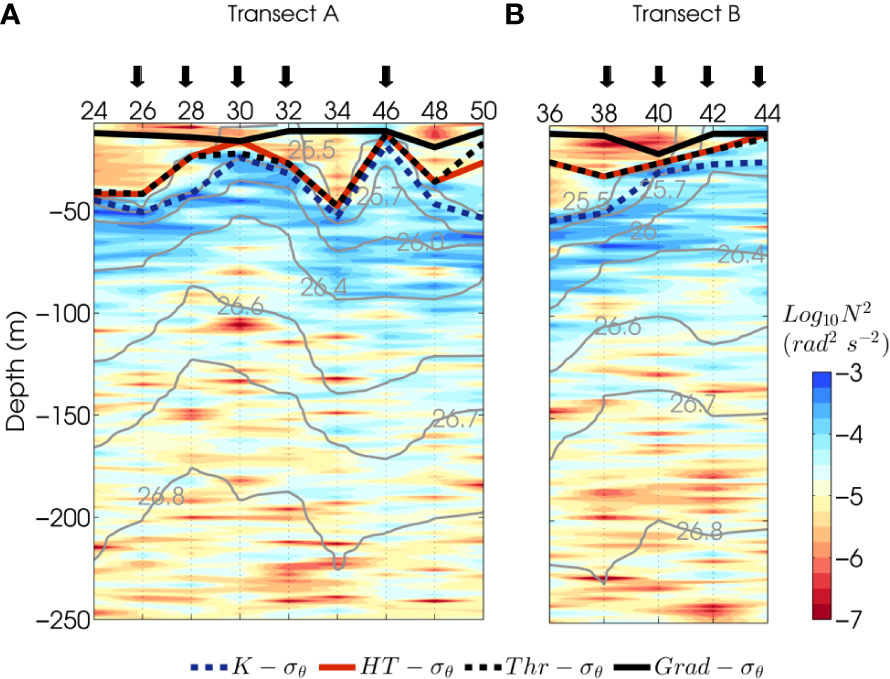
Figure 7 Vertical section of the buoyancy frequency squared (N2, rad2 s-2) in logarithmic scale for all hydrographic stations of (A) transect A and (B) transect (B) Superimposed lines indicate mixed layer depths (hρ, m) computed with different methods. For the sake of clarity, only potential density-based algorithms are shown. Squares show hρ obtained with the methods of Kara et al. (2000). Red circles show hρ obtained with the Holte and Talley (2009) algorithm (except for station 50 where a Tθ-based algorithm was more appropriate). Black squares show the σθ threshold criteria of de Boyer Montégut et al. (2004). Yellow squares show hρ computed following the gradient method of Dong et al. (2008). The light gray contours are isopycnals (σθ, m kg-3). The vertical black arrows denote the hydrographic stations of group-F, which were influenced by filament waters.
The algorithm developed by Holte and Talley (2009) can be based on the shape of either the potential density or potential temperature profile of each hydrographic station. With the exception of station 50, we found that the method from Holte and Talley (2009) resulted in an adequate fit to the observed . For station 50, the method of Holte and Talley (2009) was more appropriate, which was largely due to the existence of salinity barriers around the area caused by the subsurface salinity maximum (Pelegrí et al., 2005b). This algorithm agrees rather well with the depth of the maximum gradient of the buoyancy frequency squared (N2, rad2s-2) (Figure 7) and with the threshold method of Δσθ = 0.03 kg m-3 (de Boyer Montégut et al., 2004).
Further, we found that the algorithm given by Kara et al. (2000) tended to overestimate , whereas the gradient methods of Dong et al. (2008) tended to underestimate . These results agree with the findings of Holte and Talley (2009) for large databases of hydrographic profiles.
Several authors have emphasized the need to consider a boundary region of elevated and active mixing in the pycnocline at the base of the mixed layer (e.g., Dewey and Moum, 1990; Brainerd and Gregg, 1995; Nagai et al., 2005; Inoue et al., 2010; Sutherland et al., 2014), which is usually referred to as the mixing layer depth (). The difference between and is that the latter is the depth at which turbulent processes are active and maintain the homogeneity of the mixed layer and entrain buoyancy across the pycnocline. In contrast, represents the depth at which these surface fluxes have been mixed in the recent past (i.e., in a daily cycle or longer), thus represents the history of several mixing events. Depending on the time scale and spatial resolution, the use of could be more appropriate when evaluating entrainment than (Brainerd and Gregg, 1995). For example, fine-scale processes forced by transient mixing events in which flux conditions can change at any given moment of the day require measurements of the active mixing layer. As such, the definition of has important repercussions for Sverdrup’s critical depth theory of phytoplankton blooms (Sverdrup, 1953). Franks (2014) revisited Sverdrup’s critical depth theory and argued that , defined by density gradients, may not always reflect the intensity of active turbulence or its vertical extension. In this sense, the critical turbulence hypothesis (Huisman and Weissing, 1999) suggests that active mixing described by the definition of must be considered, as it can act to reduce stratification in the upper layer, which may lead to favorable conditions that allow phytoplankton blooms to develop (e.g., Ferrari et al., 2015).
In general, can be directly obtained with the of microstructure data (Brainerd and Gregg, 1995; Inoue et al., 2010; Franks, 2014; Sutherland et al., 2014), microstructure temperature gradients (Nagai et al., 2005), or measurements of the largest turbulent overturning length scales such as Thorpe scales (Brainerd and Gregg, 1995). In this study, we determined the base of the mixing layer when the dissipation rate decreased by two orders of magnitude from the surface, which was similarly undertaken by Inoue et al. (2010). However, not all profiles exhibited clear transitions. Therefore, a turbulent length scale, such as the Ozmidov scale (Ozmidov, 1965), could help clarify the extension of the active mixing or , where takes the following form:
In such a case, is interpreted as the size of the largest turbulent eddy in a region of stable stratification. An example of and can be viewed in Figure 8, in which the maximum vertical gradient of agrees with a decrease in of one order of magnitude within the upper boundary layer.
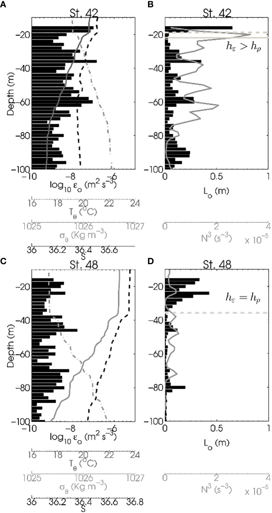
Figure 8 Vertical profiles of hydrographic and turbulent quantities. Left panels show potential temperature (Tθ °C, dark gray line), the potential density anomaly (σθ kg m-3, dash-dot line), and absolute salinity (S, dashed black line) superimposed on turbulent kinetic energy (TKE) dissipation profiles (εo m2 s-3, black bars) for (A) station 42 of group-F (within the upwelling filament) and (C) station 48 of group-nF (outside the upwelling filament). Both stations were measured during stable daytime conditions. The right panels show Ozmidov scales (Lo, m, black bars) and vertical profiles of the buoyancy frequency cubed (N3 s-3, gray profiles) for (B) station 42 and (D) station 48. Horizontal dashed and thick lines denote the mixed layer depth (hρ, m) and mixing layer depth (hε, m), respectively.
Dewey and Moum (1990), in their examination of microstructure data in upwelling filaments off northern California, noted that entrainment can only take place when exceeds ; otherwise, when mixing is not strong enough to overcome the effects of stratification in the pycnocline, entrainment cannot occur. Inoue et al. (2010) also distinguished between and to measure entrainment heat fluxes based on dissipation profiles across the Gulf Stream provided that was deeper than . The same approach was considered in this study by defining the entrainment zone or interface as .
3.4 Turbulence enhancement within upwelling filaments
When the active mixing layer extends deeper than the mixed layer, that is (Dewey and Moum, 1990; Brainerd and Gregg, 1995; Inoue et al., 2010), non-turbulent fluid from the pycnocline is subject to sufficient mixing to break stratification at the pycnocline and enters the turbulent fluid.
Some authors have speculated that enhanced turbulence below could be related to shear instabilities produced by internal waves as a result of impinging convective plumes from beneath the mixed layer (Moum et al., 1989). MacKinnon and Gregg (2005) found higher correlations between and internal wave energy than between and below the mixed layer. Here, an example of this can be seen in Figure 8, in which is deeper than for a station in group-F (Figures 8A, B). In contrast, and exhibited the same depth in a station of group-nF (Figures 8C, D). Both stations were measured during daytime conditions (i.e., during the restratification of the mixed layer when convection forcing is absent).
A complete view of active turbulent mixing is given in Figure 9, which shows vertical profiles of and superimposed profiles of scales computed for each microstructure station with their respective and . Interestingly, was deeper than (i.e., ) in filament stations (thick profiles in Figures 9, 10A, B). This suggests that only filament stations are susceptible to diapycnal entrainment by surface-forced processes (Dewey and Moum, 1990; Fer and Sundfjord, 2007; Inoue et al., 2010). This may be the result of elevated at group-F stations and the shallow mixed layers produced by isopycnal outcropping due to the isopycnal morphology of the frontal filament system.
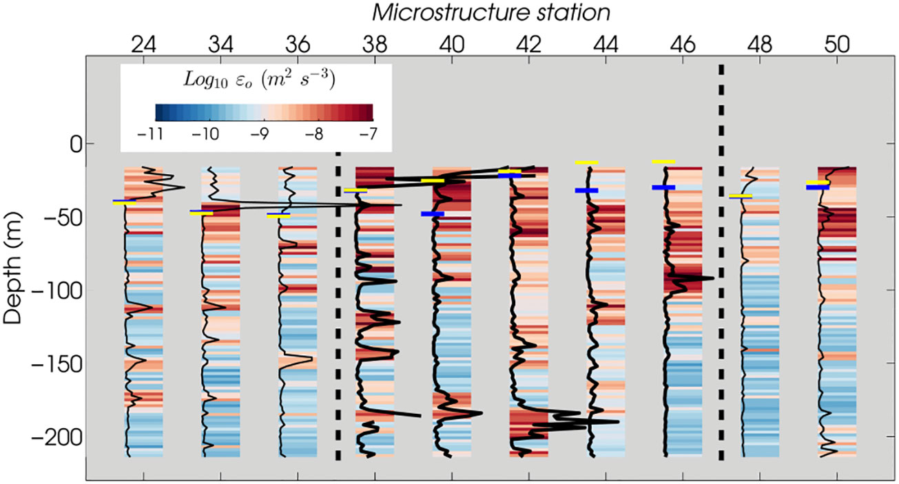
Figure 9 Vertical profiles of Ozmidov scales (Lo, m) for each microstructure station. The color columns are profiles of the observed TKE dissipation rates (εo, m2 s-3). The maximum Lo value corresponds to 5.18 m for station 34 at 42 m depth. The minimum Lo of 0.0045 m corresponds to station 38 at 66 m depth. The thick black profiles show Lo for stations of group-F. The thin profiles show Lo for stations of group-nF. The horizontal lines indicate the mixed layer depths (hρ, yellow) and mixing layer depth (hε, blue) in meters. The vertical dashed lines show the limits of the group-F stations.
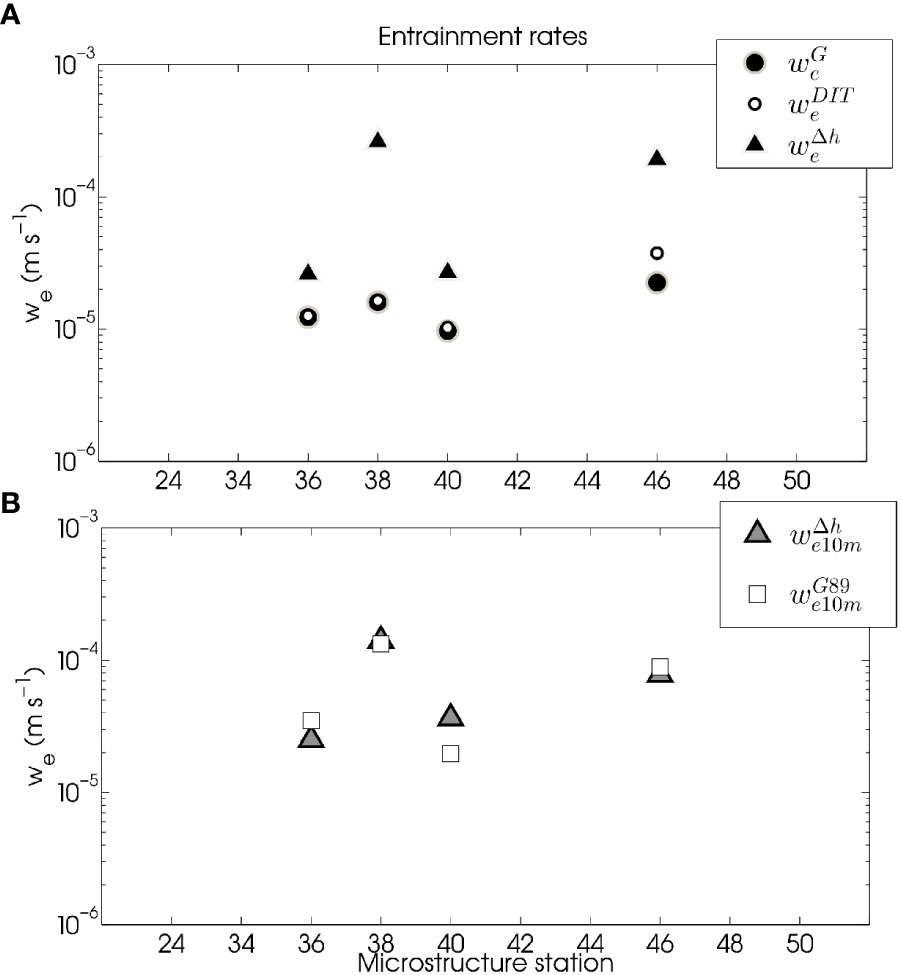
Figure 10 (A) Entrainment rates (we, m s-1) following the methodology of Gaspar (1988) (), entrainment rates adding the DIT term (), and entrainment rates using the modifications proposed in this study () computed at a vertical resolution of 2 m. (B) Entrainment rates, , averaged over 10 m for observable values (), and entrainment rates scaled following the methodology of Gregg (1989) ().
It is important to note the enhancement of below the mixed layer of filament waters, which can be seen in Figure 9. A weak wind regime during sampling days, as evidenced by the scales (Figure 4E), indicates that the turbulence generated within the upwelling filament by wind stress was likely small when compared to turbulent diapycnal buoyancy fluxes or vertical shear at the base of the mixed layer. However, this increase in turbulence has also often been linked with elevated vertical shear levels (Figure 11).
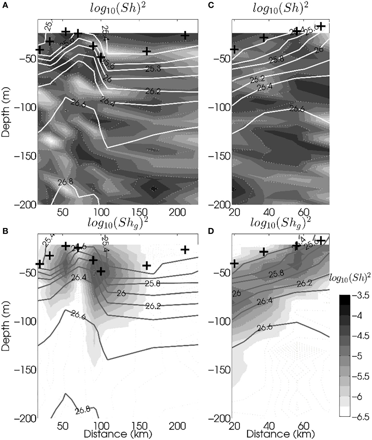
Figure 11 (A) Vertical sections of total vertical shear squared (Sh2, s-2) for transect A rotated to the reference system of geostrophic velocities and (B) geostrophic vertical shear squared (, s-2) with the level of no motion set to 650 m for transect (A) The same is shown in (C, D) for transect (B) Crosses represent the mixed layer depths (hρ, m) averaged between pairs of stations. Note the logarithmic scale. The isopycnals (kg m-3) are also shown. The cumulative distance (km) between stations is shown at the bottom.
Vertical current shear was relatively high in areas associated with isopycnal outcropping, such as in group-F stations (Figure 11), thus we examined the nature of these shear values. To ensure consistency when comparing ADCP- with geostrophic shear (), the ADCP velocities were rotated to the same reference system and interpolated between pairs of stations. Geostrophic shear was computed through the thermal wind relation by setting a reference level of no motion at 650 m (see Pelegrí et al., 2005b). In Figures 11A, C, it can be seen that the in group-F stations is mainly driven by the resolved component of the geostrophic velocity field in transect A. In transect B, the isopycnals outcropped towards the coast due to the presence of the filament and proximity to the coastal transition zone (Figure 11D). Here, the resolved geostrophic component became less relevant and ageostrophic effects arose to force total vertical shear in the stations of group-F (Figures 11B, D). These results were also supported by the geostrophic currents of altimetry data (see Figure 2). Further, the presence of a southward geostrophic current agreed with the predominance of geostrophic shear in transect A. In contrast, a departure from geostrophy appeared to take place in the coastal transition zone of transect B, in which the filament flowed southward in the opposite direction of geostrophic flow (Figure 11D), which was also observed by Dewey et al. (1993). As the filament moves offshore, it is balanced geostrophically, as was observed in transect A (Figure 11C). The enhancement of εo within the filament waters of group-F, the increase of vertical shear at the base of the mixed layer, and the resulting Δh > 0 are summarized in Figure 12.
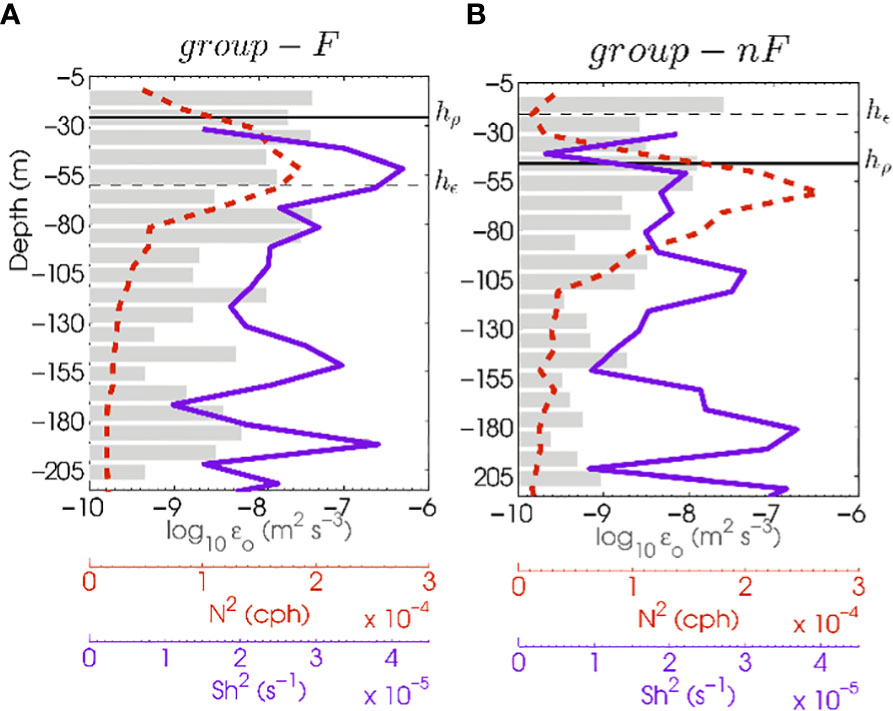
Figure 12 Horizontally averaged vertical profiles of turbulent kinetic energy (TKE) dissipation rates (εo, gray bars), buoyancy frequency squared (N2 cph, dashed red profiles), and vertical shear squared (Sh2 s-1, violet profiles) for stations of (A) group-F (where Δh > 0) and (B) stations of group-nF (where Δh > 0). The horizontal dashed and solid lines represent the average mixed layer depth (hρ) and mixing layer depth (hε, m) for both transects, respectively. Note that εo and N2 were vertically averaged to 10 m bins to ensure numerical consistency with the vertical resolution of Sh2.
In a modeling study, Small et al. (2012) argued that shear instability below the mixed layer may be generated in large part by propagating inertial waves, which ultimately increase the entrainment of cold waters from below the thermocline. Although it was not the aim of the present study to evaluate inertial wave activity, the lack of a time series of velocity currents did not allow for the presence of such near-inertial oscillations to be corroborated.
3.5 Implications of the entrainment process
The entrainment of cold, nutrient-rich waters from below the pycnocline to the surface layers and the subsequent deepening of the mixed layer are sensitive to turbulent mixing and the depth of the upper boundary layer. However, most bulk mixed layer models (Kraus and Turner, 1967; Niiler and Kraus, 1977; Gaspar, 1988) do not account for either (a) vertical shear as a source of TKE or (b) variable . Thus, such models are inappropriate for frontal areas with baroclinicity in which shallow values are driven by the rising of the pycnocline and in which breaking internal waves may be important for the generation of strong sheared flows.
Accordingly, in the case of (a), we took into account the DIT term, which is described in Eq. (5). It is assumed that turbulent entrainment can occur only when active mixing in a stratified fluid is strong enough to overcome buoyancy effects and erode the pycnocline, that is when (Dewey and Moum, 1990; Inoue et al., 2010). Given that we had direct measurements of , we restricted our analysis to stations in which was available and . In the case of (b), we considered the diapycnal turbulent buoyancy flux integrated over the entrainment zone, . This term represents a TKE sink in the entrainment zone when , as the energy is consumed when stratification breaks down. The procedure to obtain is described in Appendix A. Thus, the integration of the dissipation term over the entire active mixing layer should also be considered, similarly to what can be observed in Dewey and Moum (1990). By including these considerations in Eq. (5), the TKE-based entrainment parameterization can be described by the following equation:
Unlike other entrainment parameterizations, Eq. (8) considers TKE sources and sinks due to mechanical stirring by means of , vertical shear at the base of through the DIT term, buoyancy fluxes at the surface and turbulent buoyancy fluxes at the entrainment zone (i.e., and ), and TKE dissipation across the layer in which active mixing operates. The results from Eq. (8) yield mean entrainment rates of (~6 m d-1), which differ by a factor of 6 when compared to those of (1 m d-1) (Figure 10). The addition of the DIT term resulted in a slight increase in the entrainment rates, with a mean value of (~2 m d-1).
It is important to note that although this analysis was based on a 1D approach, several scales can coexist within ocean fronts. Two-dimensional (2D) submesoscale processes in an upwelling filament may play major roles in mixing by serving as pathways that convey the kinetic energy extracted from the mean flow to the final dissipation range throughout the secondary instabilities of the submesoscale flow (Capet et al., 2008; D’Asaro et al., 2011; Thomas et al., 2013). To determine whether this type of process affected the front in this study, the vertical distributions of potential vorticity and submesoscale energy sources were evaluated (Appendix B). As a first approximation, our results indicate that at the moment of sampling, submesoscale 2D instabilities, such as symmetric instabilities, appeared to weakly affect the frontal structure. The cross-front wind in transect A (see Figure B.1 in Appendix B) was likely insufficient to induce Ekman transport, which would cause the front to be susceptible to symmetric instabilities (e.g., D’Asaro et al., 2011). Thus, a 1D perspective based on the TKE balance is appropriate in this study. Furthermore, D’Asaro et al. (2011) indicated that although turbulent mixing near fronts can arise from these instabilities, this does not seem to be responsible for the observed elevated mixing in the Cape Ghir upwelling filament front.
3.6 Implications of the dissipation term
The TKE budget and consequently entrainment are highly sensitive to the parameterization of the dissipation term, which has proved to be a dominant sink in the energy balance (e.g., Deardorff, 1983; Gaspar, 1988; Wada et al., 2009). Our results highlight that the role of the dissipation term may be particularly important in frontal areas such as upwelling filaments. However, a dependence on observational values may make it difficult to include parameterizations of the dissipation term in bulk mixed-layer models.
We assumed a well-mixed upper ocean layer and averaged from the near-surface (far enough away from the effects of breaking waves at the surface ~16 m) to and compared this to the parameterized included in following the methods of Gaspar (1988). Our results, which are shown in Table 2, indicate that the normalized parameterized dissipation term () can be overestimated by two orders of magnitude with respect to the observed dissipation term ().
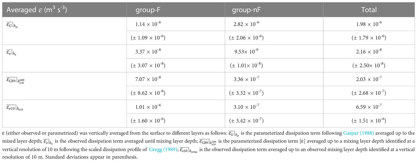
Table 2 Turbulent kinetic energy dissipation terms (ε) averaged horizontally for stations of group-F (within the filament), group-nF (outside the filament), and all microstructure stations.
In the context of a 1D TKE balance, most of the energy transferred to the interface is dissipated by viscosity. The remaining energy is stored in the form of potential energy that must work against buoyancy forces or as energy that will be subsequently converted to kinetic energy by entrainment. As a result of this 1D balance, the dissipation term may be overestimated due to entrainment velocities that are lower than expected, which suggests that the parameterized dissipation term extracts more energy from the system and leaves little energy for entrainment. Thus, decreasing the dissipation term in entrainment parameterizations to match the observed dissipation term will lead to an enhancement of . This can be seen in Figure 10, in which exhibits velocities that are higher than those given by and . This suggests that the dissipation term within the entrainment parameterization of Gaspar (1988) might not be well resolved in frontal systems.
We also compared to the internal wave scaling () proposed by Gregg (1989), which takes the internal wave spectrum into account:
where No = 5.2 × 10⁻³ (rad s-1), and SGM = 1.91 × 10⁻⁵ (s-1) is the Garret-Munk shear spectrum (Gregg, 1989).
Although the fine-scale parameterizations of differ from the observed values of , when overestimating or underestimating along the water column (Figure 13), the averaged dissipation term resembles the observed dissipation term , particularly when this is averaged within 10 m depth intervals () (Table 2). It is worth noting that the mixing layer depths obtained from are quantitatively similar to those given by the observed (Figure 10A). A comparison between mixing layer depths and the resulting entrainment zones is shown in Figures 10A, B. Note that for coarser resolutions, is always deeper than the mixed layer depth, resulting in for all stations. Moreover, the results also show agreement between and in that both show enhanced turbulent mixing in stations of group-F (Figure 13 and Table 2).
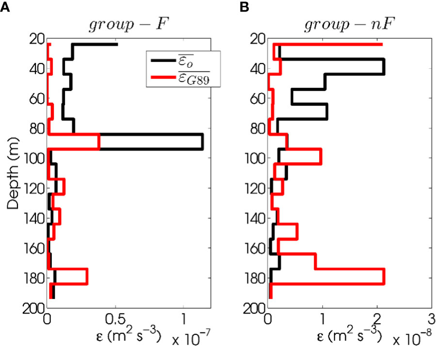
Figure 13 Comparison of turbulent kinetic energy dissipation rates, ε (m2 s-3), spatially averaged for stations of (A) group-F (within the filament) and (B) group-nF (outside the filament). Black profiles are the observed dissipation rates, (m2 s-3). The red profiles are the dissipation rates obtained following the methodology of Gregg (1989), (m2 s-3). Note the different scales of the x-axis.
These results indicate that the observed dissipation term in the proposed entrainment parameterization of Eq. (8) could be replaced by the scaling of Gregg (1989) (hereinafter ). The mean value of was 6.91 × 10⁻⁵ ± 5 × 10⁻⁵ m s-1 (6 m d-1), which is similar to , as indicated in Figure 10B. This result also suggests that the role of internal waves acting at the base of the mixed layer should not be ignored given the agreement between and .
3.7 Implications of the nutrient fluxes
It is to be expected that the enhancement of diapycnal entrainment rates observed in group-F stations would favor the elevation of deep nutrient-rich water to the photic layer. In the same study region, Arcos-Pulido et al. (2014) observed that onshore stations, which belong to group-F, exhibited diapycnal nutrient fluxes, , which were one order of magnitude greater than those observed in offshore stations calculated at a reference layer located 20 to 30 m below the mixed layer.
To verify that the enhancement of entrainment rates in the upwelling filament contributed to increasing nutrient availability below the mixed layer, we computed immediately below for each microstructure station with the following equation:
where is the diapycnal diffusivity coefficient given by the classic expression () of Osborn (1980). Buoyancy diffusivity and heat were assumed to be of the same order. The mixing efficiency (Г) is the ratio between the vertical buoyancy flux and set to 0.2 (Oakey, 1982). The nutrient concentration, which consists of the sum of nitrites and nitrates (Nut), was linearly interpolated to a vertical 2-m grid given the microstructure vertical resolution.
Nutrient gradients () were calculated over depths ranging from 5 m to 20–30 m below depending on the availability of nutrient (Schafstall et al., 2010). This differs from what was reported by Arcos-Pulido et al. (2014), who calculated fluxes for a reference layer far below . Then, was averaged for the same depth range over which was calculated. Positive values of imply an upward transport of nutrients from the pycnocline to the surface layers, where they may then be assimilated by phytoplankton.
The diapycnal nutrient fluxes (Table 3) indicated that stations of group-F exhibited large immediately below the mixed layer associated with maximal diapycnal mixing, which was three times larger than those of group-nF stations. However, station 34 was an exception to this pattern. Station 34 was located adjacent to the filament edge (see Figure 6A) and was surveyed under weak wind, non-favorable convection, and low conditions. Station 34 also exhibited more intense Lo at the mixed layer depth (Figure 9) and high nutrient gradients (Table 3) when compared to the other stations in its group. In this case, was nearly zero at station 34, indicating that both and were similar. Stations of group-F that were near station 34 (i.e., 30, 32, and 36) also exhibited high vertical nutrient gradients (not shown). This suggests that it cannot be ruled out that station 34 was influenced by either the upwelling filament or other processes, such as breaking internal waves or Langmuir cells, capable of promoting intense vertical mixing at the base of the mixed layer (Flór et al., 2010; Schafstall et al., 2010). However, the lack of microstructure observations and time series of physical variables did not allow for an evaluation of the underlying causes. Stations 48 and 50 also exhibited positive . Despite forming part of group-nF, these stations exhibited Δh > 0, indicating that favorable entrainment conditions were present, yet their fluxes were lower than those of group-F stations
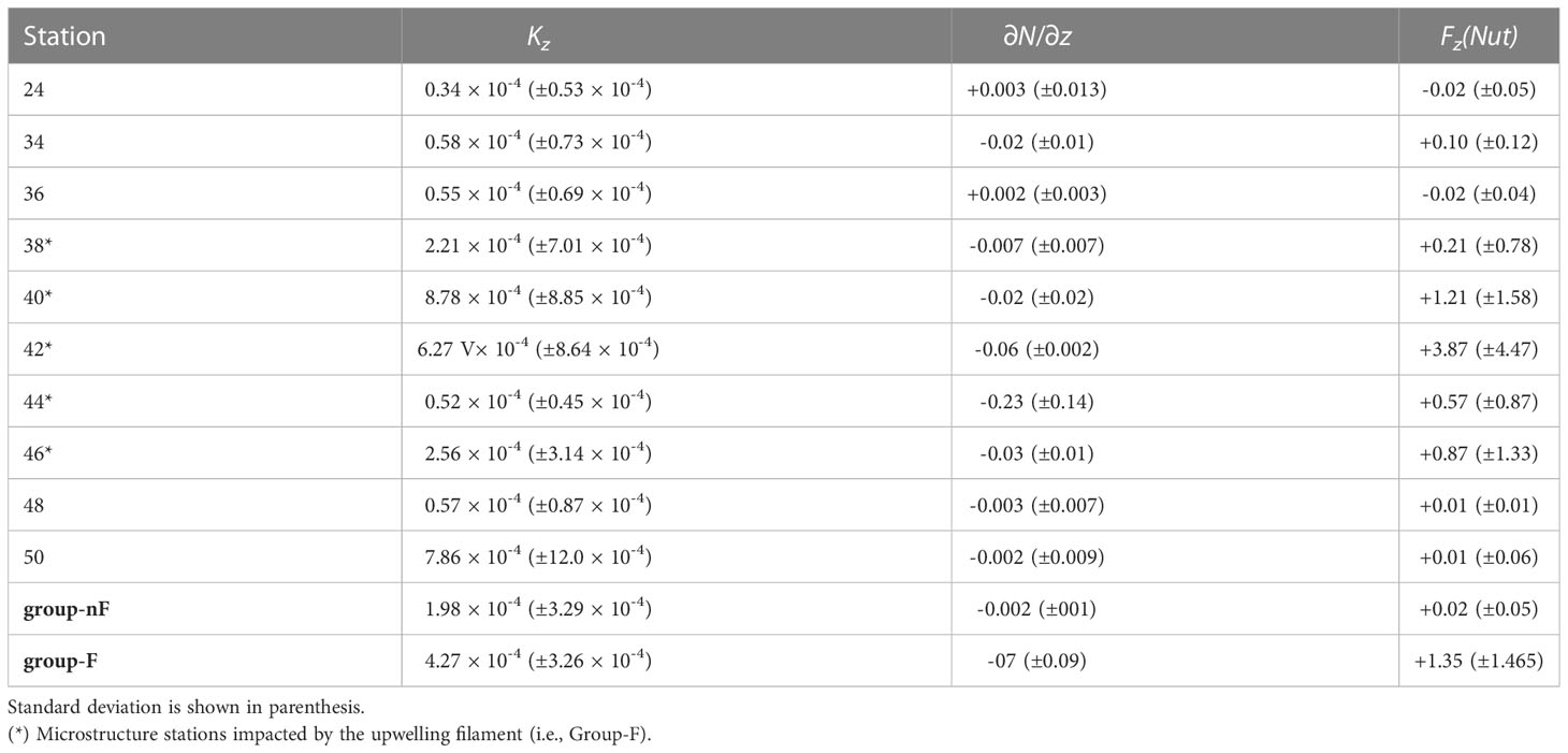
Table 3 Average values of the diapycnal diffusivity coefficient (Kz, m2 s-1), vertical nutrient gradient (nitrite + nitrate, , mmol m-4), and diapycnal nutrient flux Fz(Nut) mmol m-2 d-1) below the mixed layer for each microstructure station.
In general, stations of group-F exhibited diapycnal nutrient fluxes that were two orders of magnitude larger than those of group-nF stations. The values of for stations of group-F were at the upper end of those reported for the North Atlantic (Bahamón et al., 2003; Dietze et al., 2004; González-Dávila et al., 2006; Mouriño-Carballido et al., 2011) but of the same order of magnitude as those of other EBUS sites (Hales et al., 2005; Hales et al., 2009; Li et al., 2012). Most studies conducted in the North Atlantic have not included calculations of nutrient fluxes immediately below the mixed layer using direct microstructure observations nor in highly turbulent environments such as frontal systems. The values reported for frontal systems in other EBUS range from 5.2 (mmol m-2 d-1) in the California Current EBUS to 19.11 (mmol m-2 d-1) in the Chilean EBUS (Hales et al., 2005; Hales et al., 2009; Li et al., 2012; Corredor-Acosta et al., 2020). The latter values agree with our maxima of 8.34 (mmol m-2 d-1) for station 42 (group-F) and average of 1.35 (mmol m-2 d-1) for all stations influenced by the upwelling filament front.
4 Conclusions
We analyzed the sources and sinks of TKE that control the upper boundary layer through a simple 1D TKE-balance. This study was conducted in the submesoscale upwelling filament of Cape Ghir using satellite imagery and in-situ hydrographic measurements, including novel measurements from a microstructure profiler. The main results of this study are summarized as follows:
● Microstructure profiles revealed an enhancement of turbulent mixing within the upwelling filament front where pycnoclines shoal. The absence of strong winds and the presence of moderate buoyancy and heat fluxes enabled us to consider vertical shear as a relevant source of TKE, which is usually neglected in entrainment parameterizations.
● Enhanced turbulence and the morphology of the front promoted the formation of regions of active mixing, which were identified by the depth of the mixing layer exceeding the depth of the mixed layer, resulting in local areas of (Figures 8, 9, 12). This created optimal conditions for the entrance of nutrient-rich waters from the pycnocline to the upper boundary layer via entrainment. This theory is supported by positive values in areas directly affected by the upwelling filament in which the pycnocline is close to the surface. In such cases, turbulent mixing becomes more efficient within a smaller volume of water in the upper ocean layer. This highlights the importance of distinguishing between and .
● To quantify the role of entrainment, we included observed values of and considered , , and shear at the base of the mixed layer. We found that the entrainment rates changed considerably () and were six times greater than those of other parameterizations. We also found that the dissipation term is often overestimated. The resulting low turbulent entrainment velocities could lead to an overestimation of SST in numerical models that include such mixing schemes.
● One of the most important results of this study can be summarized by Figure 12. We found that enhanced turbulent mixing within the upwelling filament is associated with an increase in vertical shear. One possible cause of the increase in vertical shear could be the effects of internal waves, which might be particularly effective when the filament is near the coast (transect B) and vertical shear exhibits ageostrophic behavior. This also allows for to be replaced by simple scaling based on the internal wave model of Gregg (1989), , in the new proposed entrainment parameterization approach. This suggestion is supported by our result of being similar to the mean value of .
● The diapycnal nutrient fluxes presented in this study reinforce the idea that enhanced diapycnal entrainment in upwelling filaments with associated with high levels of diapycnal mixing favors the uplift of deep, nutrient-rich waters to the photic layer in submesoscale frontal systems.
This study aimed to establish a basis for future research that includes in situ data with proper spatiotemporal resolution and numerical simulations. The inclusion of additional TKE sources in entrainment studies, such as the energy of breaking internal waves that affects and turbulent Langmuir circulation, may improve our understanding of turbulence in the upper boundary layer of submesoscale fronts.
Data availability statement
The raw data supporting the conclusions of this article will be made available by the authors, without undue reservation.
Author contributions
SE-A: Write the manuscript, processing of turbulence data, atmospheric data, data analysis, parameterization, figures, and tables. ÁR-S: Expert in the diapycnal mixing process, supervised the manuscript and the processing of the data, analysis, and parameterizations. AN-G: Expert in turbulence ocean process, advised about the symmetrical instabilities process that improves the original idea and in consequence the manuscript and supervised the manuscript. LG-W: Satellite Data access and its processing of sea surface temperature and surface chlorophyll. ME: Processing of ADCP data. All authors contributed to the article and approved the submitted version.
Acknowledgments
This study was made possible by a PhD grant awarded to the first author, which was supported by the Universidad de Las Palmas de Gran Canaria. The hydrographic data necessary to reproduce this study were provided by projects PROMECA-2010 (CTM2009-06993-448 E/MAR) and PROMECA (CTM2008-04057) of Universidad de Las Palmas de Gran Canaria, co-founded by European Union (FEDER) and Ministerio de Ciencia e Inovación of Spain. The data are available from the corresponding authors upon request (angel.santana@ulpgc.es;c2hlaWxhLmVzdHJhZGExMDNAZG9jdG9yYW5kb3MudWxwZ2MuZXM=). Satellite imagery were downloaded from NASA’s Ocean Color Web for Moderate Resolution Imaging Spectroradiometer (MODIS) at NASA’s Goddard Space Flight Center. Eds. Kuring, N., Bailey, S. W. (http://oceancolor.gsfc.nasa.gov/). The altimeter products were produced by Ssalto/Duacs and distributed by Aviso, with support from Cnes (http://www.aviso.altimetry.fr/duacs/). The comments of the reviewers and editor greatly improved the manuscript. The authors also thank the captain and crew of R/V García del Cid (CSIC) as well as all participating scientists for their support during the field survey.
Conflict of interest
The authors declare that the research was conducted in the absence of any commercial or financial relationships that could be construed as a potential conflict of interest.
Publisher’s note
All claims expressed in this article are solely those of the authors and do not necessarily represent those of their affiliated organizations, or those of the publisher, the editors and the reviewers. Any product that may be evaluated in this article, or claim that may be made by its manufacturer, is not guaranteed or endorsed by the publisher.
References
Álvarez Salgado X., Arístegui J., Barton E., Hansell D. (2007). Contribution of upwelling filaments to offshore carbon export in the subtropical northeast atlantic ocean. Limnol. Oceanogr. 3 (52), 1287–1292. doi: 10.4319/lo.2007.52.3.1287
Anis A., Moum J. (1994). Prescriptions for heat flux and entrainment rates in the upper ocean during convection. J. Phys. Oceanography 24, 2142–2155. doi: 10.1175/1520-0485(1994)024<2142:PFHFAE>2.0.CO;2
Arcos-Pulido M., Rodríguez-Santana A., Emelianov M., Paka V., Benavides M., Sangrà P., et al. (2014). Diapycnal nutrient fluxes on the northern boundary of cape ghir upwelling region. Deep-Sea Res. Part I 84, 100–109. doi: 10.1016/j.dsr.2013.10.010
Bahamón N., Velasquez Z., Cruzado A. (2003). Chlorophyll a and nitrogen flux in the tropical north Atlantic ocean. Deep-Sea Res. Part I 50, 1189–1203. doi: 10.1016/S0967-0637(03)00145-6
Barton E. D., Arístegui J., Tett P., Cantón M., García-Braun J., Hernández-León S., et al. (1998). The transition zone of the canary current upwelling region. Prog. Oceanography 41, 455–504. doi: 10.1016/S0079-6611(98)00023-8
Barton E., Inall M., Sherwin T. J. (2001). Vertical structure, turbulent mixing and fluxes during Lagrangian observations of an upwelling filament system off Northwest Iberia. Prog. Oceanography 51, 249–268. doi: 10.1016/S0079-6611(01)00069-6
Berliand M. E., Berliand T. G. (1952). Measurement of the effective radiation of the earth with varying cloud amounts. Izvestiya Akademii Nauk SSSR Seriya Geofiz 1.
Brainerd K. E., Gregg M. C. (1995). Surface mixed and mixing layer depths. Geophysical Res. Lett. 42, 1521–1543. doi: 10.1016/0967-0637(95)00068-H
Capet X., McWilliams J. C., Molemaker M. J., Shchepetkin A. F. (2008). Mesoscale to submesoscale transition in the California current system. part III: energy balance and flux. J. Phys. Oceanography 38, 2256–2269. doi: 10.1175/2008JPO3810.1
Cisewski B., Strass V. H., Losch M., Prandke H. (2008). Mixed layer analysis of a mesoscale eddy in the Antarctic polar front zone. J. Geophysical Research: Oceans 113. doi: 10.1029/2007JC004372
Corredor-Acosta A., Morales C. E., Rodríguez-Santana A., Anabalón V., Valencia L., Hormazabal S. (2020). The influence of diapycnal nutrient fluxes on phytoplankton size distribution in an area of intense mesoscale and submesoscale activity off concepción, Chile. J. Geophysical Research: Oceans 125. doi: 10.1029/2019JC015539
Cronin M. F., McPhaden M. J. (1997). The upper ocean heat balance in the western equatorial pacific warm pool during september–december 1992. J. Geophysical Research: Oceans 102, 8533–8553. doi: 10.1029/97JC00020
D’Asaro E., Lee C. M., Rainville L., Harcourt R., Thomas L. N. (2011). Enhanced turbulence Energy dissipation at ocean fronts. Sci. 332, 318–332. doi: 10.1126/science.1201515
Deardorff J. W. (1970). Preliminary results from numerical integrations of the unstable boundary layer. J. Atmospheric Sci. 27, 1209–1231. doi: 10.1175/1520-0469(1970)027<1209:PRFNIO>2.0.CO;2
Deardorff J. W. (1983). A multi-limit mixed-layer entrainment formulation. J. Phys. Oceanography 13, 988–1002. doi: 10.1175/1520-0485(1983)013<0988:AMLMLE>2.0.CO;2
de Boyer Montégut C., Madec G., Fischer A. S., Lazar A., Iudicone D. (2004). Mixed layer depth over the global ocean: an examination of profile data and a profile-based climatology. J. Geophysical Res. 109. doi: 10.1029/2004JC002378
Dewey R. K., Moum J. N. (1990). Enhancement of fronts by vertical mixing. J. Geophysical Res. 95, 9433–9445. doi: 10.1029/JC095iC06p09433
Dewey R. K., Moum J. N., Caldwell D. R. (1993). Microstructure activity within a minifilament in the coastal transition zone. J. Geophysical Res. 98, 14457–14470. doi: 10.1029/93JC01127
Dickey T. C., Manov D. V., Weller R. A., Seigel D. (1994). Determination of longwave heat flux at the air–sea interface using measurements from buoy platforms. J. Atmospheric Oceanic Technol. 11, 1057–1078. doi: 10.1175/1520-0426(1994)011<1057:DOLHFA>2.0.CO;2
Dietze H., Oschlies A., Kähler P. (2004). Internal-wave-induced and double-diffusive nutrient fluxes to the nutrient-consuming surface layer in the oligotrophic subtropical north atlantic. Ocean Dynamics 54, 1–7. doi: 10.1007/s10236-003-0060-9
Dong S., Sprintall J., Gille S. T., Talley L. (2008). Southern ocean mixed-layer depth from argo float profiles. J. Geophysical Res. 113. doi: 10.1029/2006JC004051
Dorrestein R. (1979). On the vertical buoyancy flux below the sea surface as induced by atmospheric factors. J. Phys. Oceanography 9, 229–231. doi: 10.1175/1520-0485(1979)009<0229:OTVBFB>2.0.CO;2
Estrada-Allis S. N., Barceló-Llull B., Pallàs-Sanz E., Rodríguez-Santana A., Souza J. M. A. C., Mason E., et al. (2019). Vertical velocity dynamics and mixing in an anticyclone near the canary islands. J. Phys. Oceanography 49, 431–451. doi: 10.1175/JPO-D-17-0156.1
Fairall C. W., Bradley E. F., Rogers D. P., Edson J. B., Young G. S. (1996). Bulk parameterization of air-sea fluxes for tropical ocean-global atmosphere coupled-ocean atmosphere response experiment. J. Geophysical Res. 101, 3747–3764. doi: 10.1029/2010JC006884
Fer I., Sundfjord A. (2007). Observations of upper ocean boundary layer dynamics in the marginal ice zone. J. Geophysical Res. 112. doi: 10.1029/2005JC003428
Fernando H. J. (1991). Turbulent mixing in stratified fluids. Annu. Rev. Fluid Mechanics 23, 455–493. doi: 10.1146/annurev.fl.23.010191.002323
Ferrari R., Merrifield S. T., Taylor J. R. (2015). Shutdown of convection triggers increase of surface chlorophyll. J. Mar. Syst. 147, 116–122. doi: 10.1016/j.jmarsys.2014.02.009
Firing E., Ranada J., Caldwell P. (1995). Processing ADCP data with the CODAS software system version 3.1 (Joint Institute for Marine and Atmospheric Research/NODC).
Flór J. B., Hopfinger E. J., Guyez E. (2010). Contribution of coherent vortices such as langmuir cells to wind-driven surface layer mixing. J. Geophysical Res. 115. doi: 10.1029/2009JC005900
Franks P. J. (2014). Has sverdrup’s critical depth hypothesis been tested? mixed layers vs. turbulent layers. ICES J. Mar. Sci. 72, 1897–1907. doi: 10.1093/icesjms/fsu175
García-Muñoz M., Arístegui J., Pelegrí J., Antoranz A., Ojeda A., Torres M. (2005). Exchange of carbon by an upwelling filament off cape ghir (NW Africa). J. Mar. Syst. 54, 83–95. doi: 10.1016/j.jmarsys.2004.07.005
Gaspar P. (1988). Modeling the seasonal cycle of the upper ocean. J. Phys. Oceanography 18, 161–180. doi: 10.1175/1520-0485(1988)018<0161:MTSCOT>2.0.CO;2
Giordani H., Caniaux G., Voldoire A. (2013). Intraseasonal mixed-layer heat budget in the equatorial atlantic during the cold tongue development in 2006. J. Geophys. Res. Oceans 118, 650–671. doi: 10.1029/2012JC008280
González-Dávila M., Santana-Casiano M., Demetrio de Armas J., Escánez, Suarez-Tangil M. (2006). The influence of island generated eddies on the carbon dioxide system, south of the canary islands. Mar. Chem. 99, 177–190. doi: 10.1016/j.marchem.2005.11.004
Gregg M. C. (1989). Scaling turbulent dissipation in the thermocline. J. Geophys. Res. 94, 9686–9698. doi: 10.1029/JC094iC07p09686
Grodsky S. A., Carton J. A., McClain C. R. (2008). Variability of upwelling and chlorophyll in the equatorial Atlantic. Geophysical Res. Lett. 35. doi: 10.1029/2007GL032466
Hagen E. (2001). Northwest African Upwelling scenario. Oceanology Acta 24, 113–128. doi: 10.1016/S0399-1784(00)01110-5
Hagen E., Zülicke C., Feistal R. (1996). Near surface structures in the cape ghir filament off Morocco. Oceanology Acta 19, 577–598.
Hales B., Hebert D., Marra J. (2009). Turbulent supply of nutrients to phytoplankton at the new england shelf break front. J. Geophysical Res. 114. doi: 10.1029/2008JC005011
Hales B., Moum J. N., Covert P., Perlin A. (2005). Turbulent supply of nutrients to phytoplankton at the new england shelf break front. J. Geophysical Res. 110. doi: 10.1029/2004JC002685
Holte J., Talley L. (2009). A new algorithm for finding mixed layer depths with applications to argo data and subantarctic mode water formation. J. Atmospheric Oceanic Technol. 26, 1920–1939. doi: 10.1175/2009JTECHO543.1
Huffman G. D., Radshaw B. P. (1972). A note on von kármán’s constant in low reynolds number turbulent flows. J. Fluid Mechanics 53, 45–60. doi: 10.1017/S0022112072000035
Huisman J., Weissing F. J. (1999). Biodiversity of plankton by species oscillations and chaos. Nature 402, 407–410. doi: 10.1038/46540
Inoue R., Gregg M. C., Harcourt R. R. (2010). Mixing rates across the gulf stream, part 1: on the formation of eighteen degree water. J. Mar. Res. 68, 643–671. doi: 10.1357/002224011795977662
Jackson P. R., Rehmann C. R. (2014). Experiments on differential scalar mixing in turbulence in a sheared, stratified flow. J. Phys. Oceanography 44, 2661–2680. doi: 10.1175/JPO-D-14-0027.1
Jacob S. D., Shay L. K. (2003). The role of oceanic mesoscale features on the tropical cyclone-induced mixed layer response: a case study. J. Phys. Oceanography 33, 649–676. doi: 10.1175/1520-0485(2003)332.0.CO;2
Kara A. B., Rochford P. A., Hurlburt H. E. (2000). An optimal definition for ocean mixed layer depth. J. Geophysical Res. 105, 803–1682. doi: 10.1029/2000JC900072
Khanta L. H., Phillips O. M., Azadp R. S. (1977). On turbulent entrainment at a stable density interface. J. Fluid Mechanics 79, 753–768. doi: 10.1017/S0022112077000433
Kraus E. B., Turner J. S. (1967). A one-dimensional model of the seasonal thermocline II. the general theory and its consequences. Tellus 19, 98–106.
Large W. G., Pond S. (1981). Open ocean momentum flux measurements in moderate to strong winds. J. Phys. Oceanography 11, 324–336. doi: 10.1175/1520-0485(1981)011<0324:OOMFMI>2.0.CO;2
Li Q. P., Franks P. J., Ohman M. D., Landry M. R. (2012). Enhanced nitrate fluxes and biological processes at a frontal zone in the southern California current system. J. Plankton Res. 39, 790–801. doi: 10.1093/plankt/fbs006
Liu Y., Lee S. K., Muhling B. A., Lamkin J. T., Enfield D. B. (2012). Significant reduction of the loop current in the 21st century and its impact on the gulf of Mexico. J. Geophysical Res. 117. doi: 10.1029/2011JC007555
MacKinnon J. A., Gregg M. C. (2005). Spring mixing: turbulence and internal waves during restratification on the new England shelf. J. Phys. Oceanography 35, 2425–2443. doi: 10.1175/JPO2821.1
Moum J. N., Caldwell D. R., Paulson C. A. (1989). Mixing in the equatorial surface layer and thermocline. J. Geophysical Res. 94, 2005–2022. doi: 10.1029/JC094iC02p02005
Mouriño-Carballido B., Graña R., Fernández A., Bode A., Varela M., Domínguez J. F., et al. (2011). Importance of N2 fixation vs. nitrate eddy diffusion along a latitudinal transect in the Atlantic ocean. Limnol. Oceanogr. 56, 999–1007. doi: 10.4319/lo.2011.56.3.0999
Nagai T., Yamazaki H., Nagashima H., Kantha L. H. (2005). Field and numerical study of entrainment laws for surface mixed layer. Deep-Sea Res. Part II 52, 1109–1132. doi: 10.1016/j.dsr2.2005.01.011
Niiler P. P., Kraus E. B. (1977). One-dimensional model ofthe upper ocean. modelling and prediction of the upper layers of the ocean. Ed. Kraus E. B. (Pergamon Press.), 143–172.
Oakey N. S. (1982). Determination of the rate of dissipation of turbulent energy from simultaneous temperature and velocity shear microstructure measurements. J. Phys. Oceanography 12, 256–271. doi: 10.1175/1520-0485(1982)012<0256:DOTROD>2.0.CO;2
Osborn T. R. (1980). Estimates of the local rate of vertical diffusion from dissipation measurements. J. Phys. Oceanography 10, 83–89. doi: 10.1175/1520-0485(1980)010<0083:EOTLRO>2.0.CO;2
Ozmidov R. V. (1965). On the turbulent exchange in a stably stratified ocean. Atmospheric Oceanic Phys. 8, 853–860.
Pelegrí J. L., Arístegui J., Cana L., González-Dávila M., Hernández-Guerra A., Hernández-León S., et al. (2005a). Coupling between the open ocean and the coastal upwelling region off Northwest Africa: water recirculation and offshore pumping of organic matter. J. Mar. Syst. 54, 3–37. doi: 10.1016/j.jmarsys.2004.07.003
Pelegrí J. L., Marrero-Díaz A., Ratsimandresy A., Antoranz A., Cisneros-Aguirre J., Gordo C., et al. (2005b). Hydrographic cruises off Northwest Africa: the canary current and the cape ghir region. J. Mar. Syst. 54, 39–63. doi: 10.1016/j.jmarsys.2004.07.001
Pelegrí J. L., Richman J. G. (1993). On the role of shear mixing during transient coastal upwelling. Continental Shelf Res. 13, 1363–1400. doi: 10.1016/0278-4343(93)90088-F
Peng J., Holtermann P., Umlauf L. (2020). Frontal instability and energy dissipation in a submesoscale upwelling filament. J. Phys. Oceanography 7. doi: 10.1175/JPO-D-19-0270.1
Ravindran P., Wright D. G., Platt T., Sathyendranath S. (1999). A generalized depth-integrated model of the oceanic mixed layer. J. Phys. Oceanography 29, 791–806. doi: 10.1175/1520-0485(1999)029<0791:AGDIMO>2.0.CO;2
Samson G., Giordani H., Caniaux G., Roux F. (2009). Numerical investigation of an oceanic resonant regime induced by hurricane winds. Ocean Dynamics 59, 565–586. doi: 10.1007/s10236-009-0203-8
Sangrà P., Pascual A., Rodríguez-Santana A., Machín F., Mason E., McWilliams J. C., et al. (2009). The canary eddy corridor: a major pathway for long-lived eddies in the subtropical north Atlantic. Deep Sea Res. Part I 56, 2100–2114. doi: 10.1016/j.dsr.2009.08.008
Sangrà P., Troupin C., Barreiro-González B., Barton D. E., Abdellatif O., Arístegui J. (2015). The cape ghir filament system in august 2009 (NW Africa). J. Geophysical Research: Oceans 120, 4516–4533. doi: 10.1002/2014JC010514
Santana-Falcón Y., Mason E., Arístegui J. (2020). Offshore transport of organic carbon by upwelling filaments in the canary current system. Prog. Oceanography 186, 2100–2114. doi: 10.1016/j.pocean.2020.102322
Schafstall J., Dengler M., Brandt P., Bange H. (2010). Tidal induced mixing and diapycnal nutrient fluxes in the Mauritanian upwelling region. J. Geophysical Res. 115, 1978–2012. doi: 10.1029/2009JC005940
Small R. J., Carniel S., Campbell T., Teixeira J., Allard R. (2012). The response of the ligurian and tyrrhenian seas to a summer mistral event: a coupled atmosphere–ocean approach. Ocean Model. 48, 30–44. doi: 10.1016/j.ocemod.2012.02.003
Strang E. J., Fernando H. J. S. (2001). Entrainment and mixing in stratified shear flows. J. Fluid Mechanics 428, 349–386. doi: 10.1017/S0022112000002706
Sun J., Wang Y. (2008). Effect of the entrainment flux ratio on the relationship between entrainment rate and convective Richardson number. Boundary-Layer Meteorology 126, 237–247. doi: 10.1007/s10546-007-9231-4
Sutherland G., Reverdin G., Marié L., Ward B. (2014). Mixed and mixing layer depths in the ocean surface boundary layer under conditions of diurnal stratification. Geophysical Res. Lett. 41, 8469–8476. doi: 10.1002/2014GL061939
Sverdrup H. U. (1953). On conditions for the vernal blooming of phytoplankton. J. du Conseil Int. pour l’Exploration la Mer 18, 287–295.
Thomas L. N., Taylor J. R., Ferrari R., Joyce T. M. (2013). Symmetric instability in the gulf stream. Deep-Sea Res. Part II 91, 96–110. doi: 10.1016/j.dsr2.2013.02.025
Troupin C., Mason E., Beckers J. M., Sangrà P. (2012). Generation of the cape ghir upwelling filament: a numerical study. Ocean Model. 41, 1–15. doi: 10.1016/j.ocemod.2011.09.001
Wada A., Niino H., Nakano H. (2009). Roles of vertical turbulent mixing in the ocean response to typhoon Rex, (1998). J. Oceanography 65, 373–396. doi: 10.1007/s10872-009-0034-8
Wade M., Caniaux G., duPenhoat Y., Dengler M., Giordani H., Hummels R. (2011). A one-dimensional modeling study of the diurnal cycle in the equatorial atlantic at the pirata buoys during the egee–3 campaign. Ocean Dynamics 61, 1–20. doi: 10.1007/s10236-010-0337-8
Wolk F., Yamazaki H., Seuront L., Lueck R. G. (2002). A new free-fall profiler for measuring biophysical microstructure. J. Atmospheric Oceanic Technol. 19, 780–793. doi: 10.1175/1520-0426(2002)019<0780:ANFFPF>2.0.CO;2
Zaron E. D., Moum J. N. (2009). A new look at Richardson number mixing schemes for equatorial ocean modeling. J. Phys. Oceanography 39, 2652–2664. doi: 10.1175/2009JPO4133.1
Appendix A.
According to Osborn (1980), the diapycnal turbulent buoyancy flux () can be scaled as:
where the mixing efficiency (Г) is the ratio of the vertical buoyancy flux to . We employed a constant value of 0.2 (e.g., Zaron and Moum, 2009). To consider the diapycnal turbulent buoyancy flux that contributes to the TKE budget in the entrainment zone, a parameterization derived from Osborn (1980) was integrated over the entrainment zone, (i.e., from to ) to obtain :
Due to the dependence on , is only a TKE sink when , thus it will be a sink in filament waters given that energy is consumed to break stratification below the mixed layer.
Appendix B. Submesoscale Processes
Turbulence is a three-dimensional (3D) process. To restrict the entrainment analysis to a 1D approach, we required a prior examination of 2D instabilities that could occur in frontal structures.
Following the analysis of Thomas et al. (2013), potential vorticity (q) can be determined as for transect A and similarly as for transect B. Despite the lack of synoptic measurements, an analysis of q revealed positive values for along-front qA (Figure B.1A, indicating stable conditions (e.g., D’Asaro et al., 2011). Transect B (Figure B.1B) exhibited a similar pattern to that of transect A in the along-front qB, with slightly near zero values at locations where isopycnals outcropped to the surface and (i.e., at the upwelling filament). These results provide no immediate evidence for symmetric instabilities, which was supported by the presence of cross-front winds in transect A (Figure B.1). This indicates that a 1D turbulent approach is appropriate for this case study.
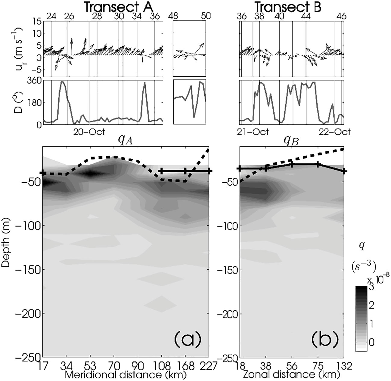
Figure B.1 Upper panels: wind speed (ur, m s-1) with the respective wind direction (clockwise from North). Lower panels: cross-stream sections of potential vorticity (q, s-3) for (A) transect A and (B) transect B. The dashed lines correspond to mixed layer depths (hρ). The solid lines denote mixing layer depths (hε, m).
Keywords: upwelling filament, diapycnal mixing, active mixing, turbulent, entrainment, entrainment parameterization
Citation: Estrada-Allis SN, Rodríguez-Santana Á, Naveira-Garabato AC, García-Weil L, Arcos-Pulido M and Emelianov M (2023) Enhancement of turbulence and nutrient fluxes within an Eastern Boundary Upwelling Filament: a diapycnal entrainment approach. Front. Mar. Sci. 10:1113879. doi: 10.3389/fmars.2023.1113879
Received: 01 December 2022; Accepted: 15 May 2023;
Published: 17 July 2023.
Edited by:
Weifeng (Gordon) Zhang, Woods Hole Oceanographic Institution, United StatesReviewed by:
Jonathan Nash, Oregon State University, United StatesShuang-Xi Guo, Chinese Academy of Sciences (CAS), China
Copyright © 2023 Estrada-Allis, Rodríguez-Santana, Naveira-Garabato, García-Weil, Arcos-Pulido and Emelianov. This is an open-access article distributed under the terms of the Creative Commons Attribution License (CC BY). The use, distribution or reproduction in other forums is permitted, provided the original author(s) and the copyright owner(s) are credited and that the original publication in this journal is cited, in accordance with accepted academic practice. No use, distribution or reproduction is permitted which does not comply with these terms.
*Correspondence: Sheila N. Estrada-Allis, c2hlaWxhQGNpY2VzZS5teA==