Data augmentation and deep neural network classification based on ship radiated noise

Introduction: Various types of ships sail at sea, and identifying maritime ship types through shipradiated noise is one of the tasks of ocean observation. The ocean environment is complex and changeable, such rapid environmental changes underline the difficulties of obtaining a huge amount of samples. Meanwhile, the length of each sample has a decisive influence on the classification results, but there is no universal sampling length selection standard.

Methods: This study proposes an effective framework for ship-radiated noise classification. The framework includes: i) A comprehensive judgment method based on multiple features for sample length selecting. ii) One-dimensional deep convolution generative adversarial network (1-DDCGAN) model to augment the training datasets for small sample problem. iii) One-dimensional convolution neural network (CNN) trained by generated data and real data for ship-radiated noise classification. On this basis, a onedimensional residual network (ResNet) is designed to improve classification accuracy.

Results: Experiments are performed to verify the proposed framework using public datasets. After data augmentation, statistical parameters are used to measure the similarity between the original samples and the generated samples. Then, the generated samples are integrated into the training set. The convergence speed of the network is clearly accelerated, and the classification accuracy is significantly improved in the one-dimensional CNN and ResNet.

Discussion: In this study, we propose an effective framework for the lack of scientific sample length selection and lack of sample number in the classification of ship-radiated noise, but there aret still some problems: high complexity, structural redundancy, poor adaptability, and so on. They are also long-standing problems in this field that needs to be solved urgently.

1 Introduction

Ship-radiated noise is the unavoidable noise emitted by ships during movement. Traditional classification for ship-radiated noise mainly relies on the artificial extraction of features, such as time, frequency and time-frequency domain characteristics Zhang et al. (2020a).

Ship-radiated noise is generally modelled as a composition of mechanical, hydrodynamic and propeller noise components Yan et al. (2021); Zhang and Yang (2022). Mechanical noise is generated by diesel engines, the generators and air condition units, and mainly comprises line spectra Zhang et al. (2020b). Hydrodynamic noise is a time-stationary signal with a continuous spectrum. Considered environmental noise, as well as multi-path and Doppler effects in the propagation process, which make ship-radiation noise an unstable process with nonlinear, non-Gaussian and non-stationary characteristics Zhang et al. (2022b).

With the development of noise reduction technology, the distinguishing features have been significantly weakened, which increases the difficulty of collecting data. Meanwhile, the sample size in existing publicly available dataset is small. Most researchers commonly use feature extraction algorithms to solve this problem Qi et al. (2020); Zhang et al. (2021). In this paper, on the basis of traditional feature extraction and data augmentation Ian et al. (2014), a new idea of noise data augmentation is proposed to deal with the problem of small sample sizes in ship-radiated noise classification.

Traditional approaches in ship-radiated noise classification with small sample size are based on an analysis of machine learning Li et al. (2019); Xie et al. (2020). The core steps are to extract the features of the signal, increase the differences between different samples, and use these features to identify or classify signals Pethiyagoda et al. (2018). In earlier works, researches classify the signal using amplitude and frequency content Yang et al. (2021). Based on the difficulties of effective features extracting, some researchers start to use artificial feature extraction techniques, such as principal component analysis Wei (2016).

In Li et al. (2019), Support vector machine (SVM) is used for ship classifying because its ability to perform non-linear classification. In Xie et al. (2020), permutation entropy is combined with the normalized correlation coefficient and enhanced variational mode decomposition, and an SVM is used to classify three types of ships. In Jiao et al. (2021), fluctuation-based dispersion entropy is combined with intrinsic time-scale decomposition, and SVM is used for classification. The common classification methods are compared in Table 1. GAN is proposed by Goodfellow et al. Ian et al. (2014) for solving the imbalanced data problem. It is used in many fields Arniriparian et al. (2018). In Atanackovic et al. (2020), authors use GAN to augment ship-radiated noise data. In this study, we augment ship-radiated noise data using GAN models to obtain sufficiently similar and diverse samples.

TABLE 1

Table 1 Comparison of common ship-radiated noise classification methods.

With the development of neural networks in recent years, faster convergence times and higher accuracy have been achieved. This requires large amounts of balanced data to fully train the deep network structures. Some researchers have focused on manually extracted features combined with SVMs for ship-radiated noise classification Li and Yang (2021). If the number of samples is small or there is a big gap in the proportion of different samples, then there will be reduced classification accuracy Buda et al. (2018). When considering a one-dimensional speech signal, the length of the sample needs to be considered Zhang et al. (2022c). Under normal circumstances, collected ship-radiated noise is a piece of audio, which needs to be split, and thus the appropriate length of each sample needs to be determined. In this paper, we propose a comprehensive judgment method based on multiple features to select an appropriate sample length. The model used for data augmentation and the deep neural networks are designed with the selected sample length.

In Pan et al. (2019), two ways are proposed for the optimization GAN models: architecture optimization and objective function optimization. Convolutional neural networks (CNNs) are a kind of network that can adaptive extract the characteristics of the signal Zhang et al. (2022a). Moreover, there are also deep features extracted by convolution that cannot be easily extracted manually. For the above reasons, we choose convolution-based GANs for structural optimization. Convolution-based GANs are a development of CNNs, and DCGAN is one of the main models used Arniriparian et al. (2018). However, these GAN models are mostly used in the two-dimensional image processing domain. Based on DCGAN, in this paper we propose a one-dimensional DCGAN (1-DDCGAN) to generate ship-radiated noise samples.

In summary, in this paper, by using the public dataset ShipsEar Santos-Domínguez et al. (2016), we propose a data augmentation method with a comprehensive length select algorithm. Then, construct a deep neural framework for ship classification. The main contributions can be summarized as follows:

1. A new classification method is proposed, which is based on deep neural network classification combined with data augmentation. The proposed method is capable of performing accurate classification in the presence of small numbers of training samples.

2. We propose a decision-level fusion method to select sample length and combine 1-DDCGAN and ResNet for data augmentation and feature classification without manual feature extraction. The convergence time is reduced Xie et al. (2020) and the classification accuracy is improved Li et al. (2017); Li et al. (2019).

3. The performance of the proposed method is verified using experimental data Santos-Domínguez et al. (2016). First, data augmentation is carried out and the generated sample is mixed with the original in different proportions to increase the number of sample in training sets. From using only the original sample to a ratio of the original sample to the generated sample being 1:2, the classification rate in CNN improved from 79% to 90%, while the classification rate in ResNet improved from 87.5% to 99.17%.

The overall approach is shown in Figure 1. The rest of this paper is organized as follows. In Section 2, we discuss cepstrum coefficients and entropy characteristics. Then, an SVM is used for classification in order to determine the appropriate sample length. A 1-DDCGAN is then designed and the generated augmentation data are analyzed in Section 3. Section 4 describes merging the real and generated data in different proportions, and the classification accuracy under these training sets is compared. Conclusions are provided in Section 5.

FIGURE 1

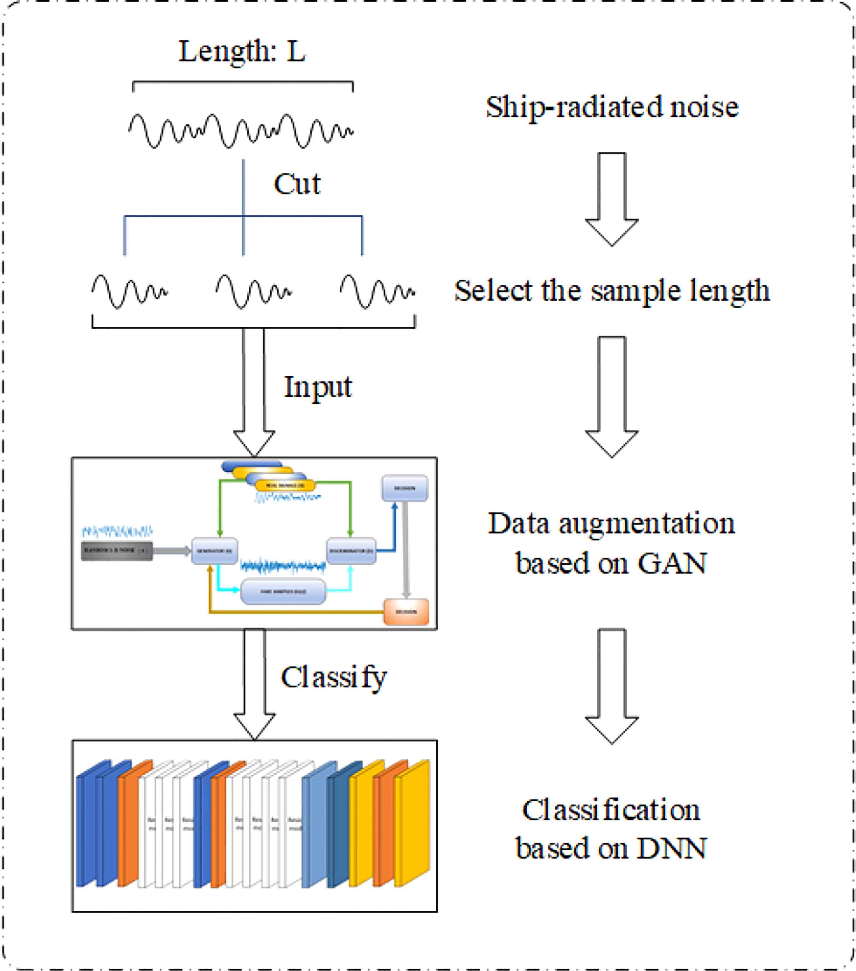
Figure 1 General algorithm framework.

2 Sample length selection of ship-radiated noise

The cepstrum coefficients and entropy features reflect different aspects of the signal characteristics. In order to extract different aspects of the information contained in the signal, we select the appropriate sampling length according to the contribution of these characteristics in the classification process. The details are shown in Figure 2.

FIGURE 2

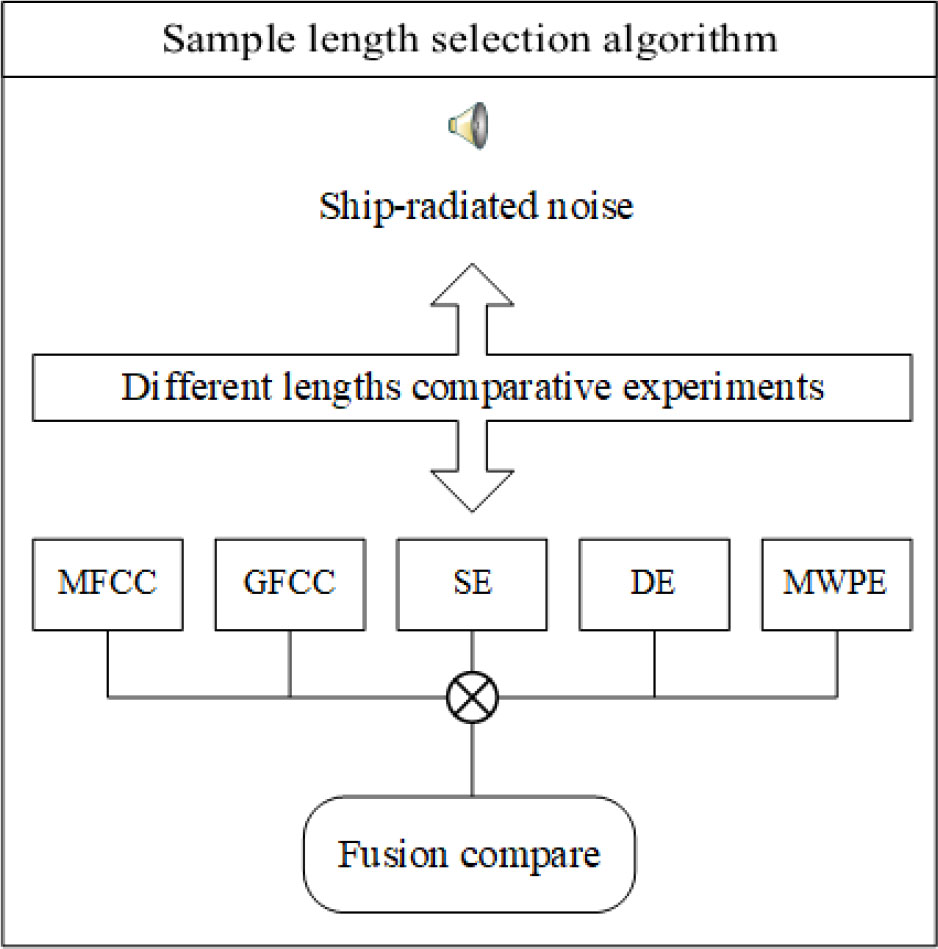
Figure 2 Sample length selection algorithm framework.

Mel-frequency cepstrum coefficient (MFCC)-based features reflect the timbre of the signal Noda et al. (2019), while Gammatone cepstrum coefficients (GFCC)-based features reflect the robustness, the degree of influence of data disturbance, noise, and outliers in the model Zhang et al. (2018). On the other hand, entropy-based features describe the extent of signal regularity, which can be useful for the classification of nonlinear non-stationary ship-radiated noise. These characteristics can be used to measure the amount of information contained in the sample from many aspects. Sample entropy measures the complexity of a time series by measuring the probability of encountering new patterns in the signal Richman et al. (2004). Specifically, dispersion entropy is more suitable for long signals and represents the amplitude characteristics of the signals. Multi-scale weighted permutation entropy can retain the amplitude information of the signal when calculating the sequential mode of the time series Shi et al. (2021). Since these features reflect different characteristics of signals, we selected them for comprehensive consideration and selection of an appropriate sample length of ship-radiated noise. Meanwhile, when the GAN is used for sample generation, GAN uses random noise as input to generate, longer inputs require longer iteration times, so longer sample lengths lead to longer computation times. The purpose of sample length selection is to determine the optimal trade-off between having sufficient features while maintaining the computational load to a minimum.

2.1 Cepstrum coefficient characteristics

MFCC is a characteristic parameter based on the characteristics of simulated acoustic signals passing through the cochlea Lin et al. (2021). The Mel scale describes the nonlinear characteristics of human ear frequencies, and MFCC is the cepstrum coefficient extracted under the nonlinear characteristics of this frequency. The relationship between frequency and the Mel scale can be approximated using the following equation:

$\begin{array}{ll}M(f)=2595log(1+f/700)& (1)\end{array}$

where f is the frequency of the signal, while the other fixed parameters are derived from the cochlea. The specific steps of the algorithm are shown in Figure 3:

FIGURE 3

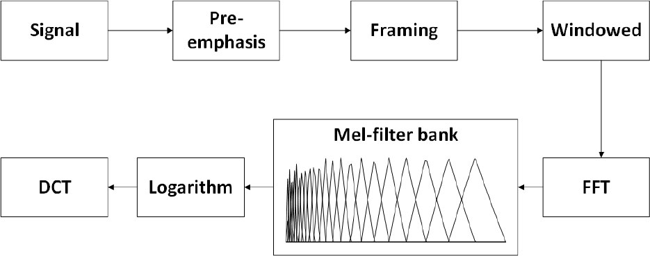
Figure 3 MFCC algorithm flow chart.

In Figure 3, the signal is pre-weighted through a high-pass filter and divided into frames with a length of 256, while a Hamming window is applied to each frame to enhance the continuity at both ends. Next, a fast Fourier transform is applied on these frames, which then pass through the triangular filter banks based on the Mel scale. After that, the logarithmic energy of each filter output is calculated and the discrete cosine transform (DCT) is applied to finally obtain MFCC feature.

The Gammatone filter simulates the spectrum analysis and frequency selection characteristic of human ears to achieve strong noise resistance and maintain good classification performance in environments with strong interference. It is a bandpass filter, defined in time domain as:

$\begin{array}{ll}g(t,f_c)=A{t}^{n-1}{e}^{-2\pi bt}\cos (2\pi f_{c}t+\varphi )& (2)\end{array}$

where n is the filter order, A is the filter gain, b is the filter attenuation factor, f_c is the center frequency, and φ is the filter phase.

A Gammatone filter bank is formed using a series of Gammatone filter combinations with different center frequencies [282018Zhang et al.Zhang, Wu, Wang, Wang, Wang, and Zhang]. The center frequencies are first obtained by dividing the equivalent bandwidth scale in equal parts, and are then mapped to a linear scale to determine the center frequency of each Gammatone filter. After that, the characteristic GFCC parameters can be obtained using a logarithmic operation and the DCT. The detailed process is shown in Figure 4.

FIGURE 4

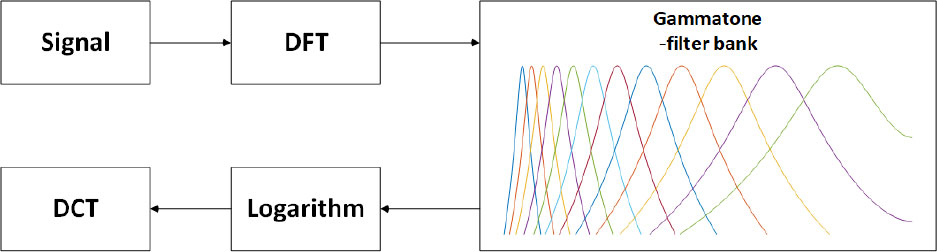
Figure 4 GFCC algorithm flow chart.

2.2 Entropy feature

In this section, we describe sample entropy, dispersion entropy and multi-scale weighted permutation entropy.

2.2.1 Sample entropy

Sample entropy is a nonlinear entropy metric commonly used to describe complexity Richman et al. (2004). Sample entropy measures the likelihood of the occurrence of a new pattern in a time series, that is, it is a prediction of the amplitude distribution of future signals based on the current amplitude distribution. In essence, it is the quantification of the complexity and regularity of a sequence. The algorithm is described in Algorithm 1.

ALGORITHM 1SAMPLE ENTROPY.

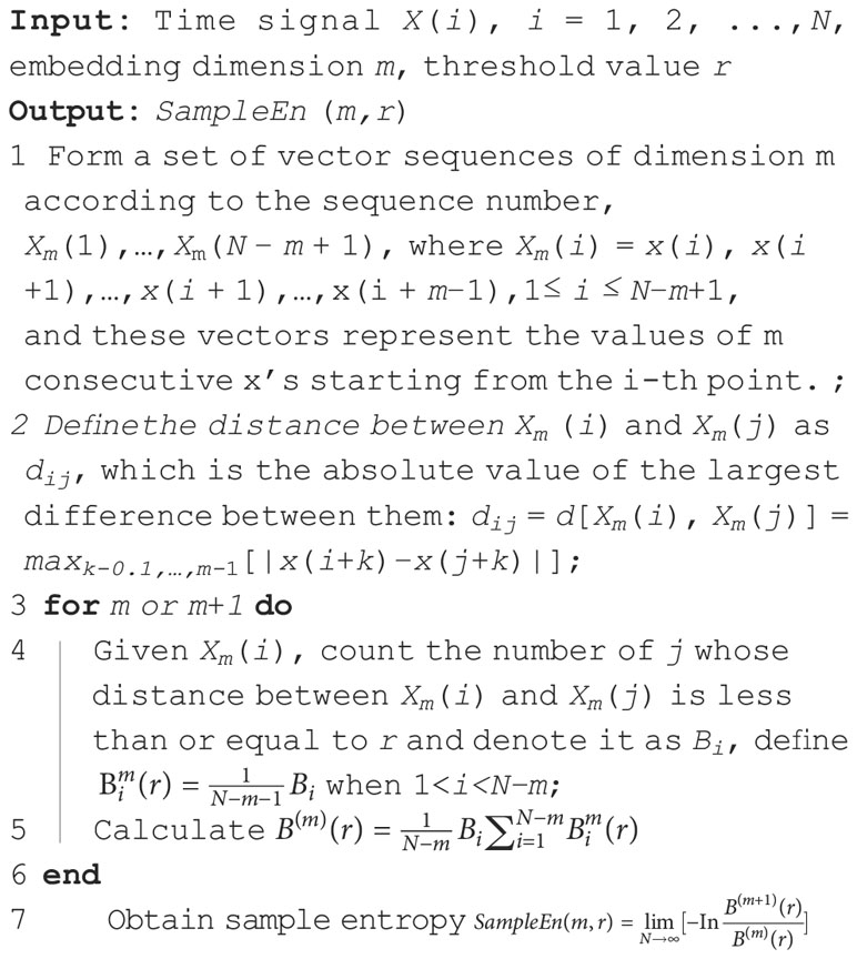
Algorithm 1Sample Entropy..

2.2.2 Dispersion entropy

Dispersion entropy is a metric used to measure the complexity and irregularity of time series, which is sensitive to the variation of the frequency, amplitude, and time series’ bandwidth, and it does not require the sorting of the amplitude values of each embedded vector Li et al. (2022). Because of the above characteristics, the calculation efficiency of the dispersion entropy is high. The calculation steps of dispersion entropy are given in Algorithm 2.

ALGORITHM 2 DISPERSION ENTROPY.

Algorithm 2 Dispersion Entropy..

2.2.3 Multi-scale weighted permutation entropy

Permutation entropy (PE) is suitable for time series, because it measures their randomness and detects their dynamic changes. It can be obtained at fast speeds through a comparison of neighboring values. Weighted PE (WPE) is an improved algorithm based on PE, which fully considers that the amplitude of adjacent vectors of the same order may be different. PE and WPE are already used in different fields, such as underwater acoustic signal denoising Li et al. (2018). The detailed calculation steps are described in Algorithm 3.

ALGORITHM 3 WEIGHTED PERMUTATION ENTROPY.

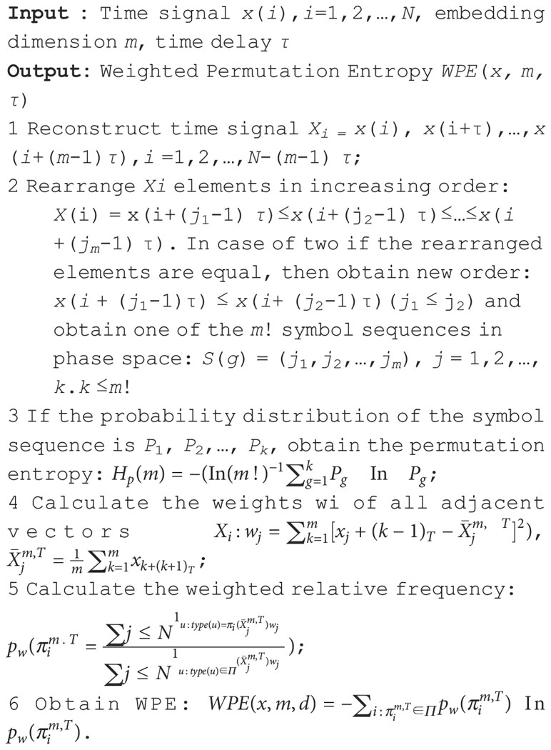
Algorithm 3 Weighted Permutation Entropy..

The multi-scale analysis algorithm is developed by Costa, and can be used to estimate the complexity of the original data at different scales Chen et al. (2019). Based on the concept of multi-scale analysis, multi-scale permutation entropy (MPE) is proposed by Aziz and Arif (2005). The MPE algorithm is divided into two steps. The first step is the application of a coarse-grained procedure to obtain multi-scale time series from the original time series. The second step is the calculation of the WPE at each coarse-grained time series. The details of the algorithm are shown in Algorithm 4.

ALGORITHM 4 MULTI-SCALE WEIGHTED PERMUTATION ENTROPY.

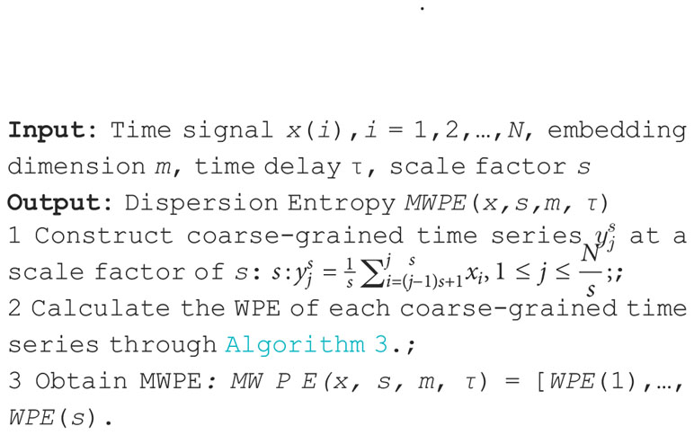
Algorithm 4 Multi-scale Weighted Permutation Entropy..

2.3 Experimental results

In the ship-radiated noise generated by the four types of ships, we randomly selected 64 samples for each type, used 200 of the 256 samples as the training set and 56 as the test set for classification, and analyzed the classification results under different sample lengths. Support vector machine can achieve good classification results in a short time in the case of fewer samples and manual feature extraction. We used MFCC, GFCC, MWPE, SE, and DE to express different characteristics of signals for feature extraction, and the corresponding features are independently input into the SVM classifier, starting from a sample length of 100 sampling points and up to 2,500 sampling points at an interval of 100 sampling points.

Figure 5 shows the classification results for the above-mentioned features. In classification using MFCC, 256 or 512 sampling points are usually used as a frame when framing. We selected 256 sampling points as a basic frame. The algorithm cannot work when the sampling length is less than two basic frames, the classification rate is 0 when the sampling length is less than 500 sampling points. When the sample length increases, the classification accuracy of each feature also improves. At this time, the sample length has a greater impact on classification. The classification rate tends stabilize when the sample length is about 1,600 sampling points. We concluded that the ship-radiated noise sample at this time already contained enough information for classification. In a CNN, the time complexity of a single convolutional layer is TimeO(M² K² C_inC_out), where M is the side length of the convolution kernel; K is the side length of the convolution kernel; C_in is the number of input channels; C_out is the number of output channels; and the size of the output feature map M itself is determined by four parameters, the input matrix size X, the size of the convolution kernel K, Padding, and Stride, which are expressed as M=(X−K+2∗Padding)/Stride+1. The space complexity of the CNN is determined by the total parameter amount and the feature map output by each layer as follows: $Space\sim O({\displaystyle {\sum }_{l=1}^D{K}^{2_l}·}{C}_{l-1}·C_l+{\displaystyle {\sum }_{l=1}^D{M}^2}·C_l)$ .The total parameter amount is only related to the size of the convolution kernel K, the number of channels C, and the number of layers D; it has nothing to do with the size of the input data. The space occupation of the output feature map is related to the space size M and the number of channels C. In other words, the performances of the network are closely related to the input size. The sampling length we selected after a comprehensive analysis of multiple features is 1,600 sampling points. A sample of this size can not only reduce the time and space complexity of the network but also obtain results efficiently and prevent overfitting.

FIGURE 5

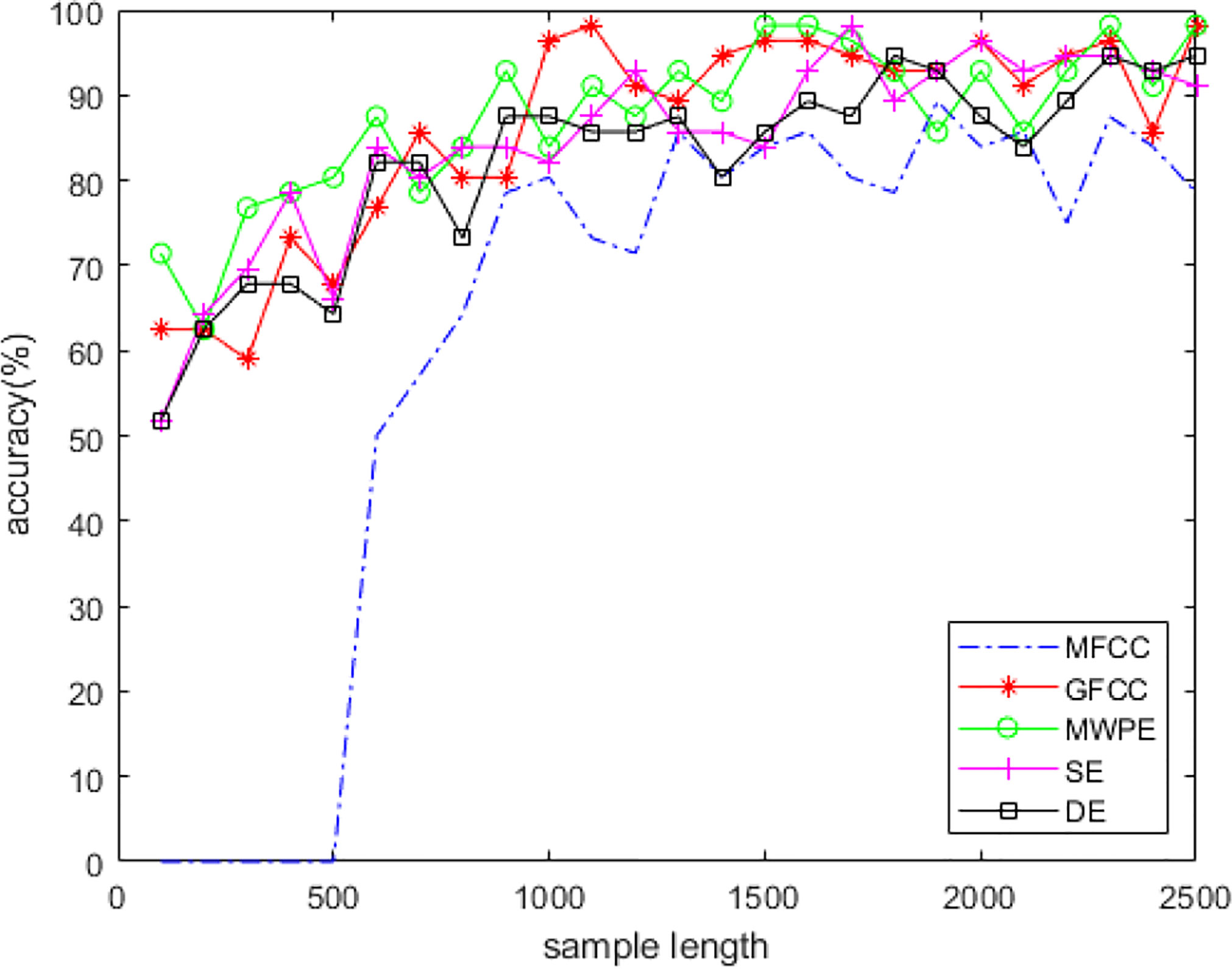
Figure 5 Classification results of different features.

3 1-DDCGAN for ship-radiated noise data augmentation

When training deep neural networks, too few training samples results in limited features learned by the network, making it difficult to perform more complex classification tasks. We used 1-DDCGAN to enhance the data and analyze the generated samples.

3.1 1-DDCGAN structure

GANs provide a way to learn deep representations without extensive annotated training data by using backpropagation through a competitive process involving a pair of networks. GANs are used in a variety of applications, including image synthesis, semantic image editing, style transfer, image super-resolution, and classification Arniriparian et al. (2018); Pan et al. (2019). GANs are inspired by the game theory, where the generator and discriminator will compete with each other to achieve a Nash equilibrium during training. The architecture of GAN is shown in Figure 6.

FIGURE 6

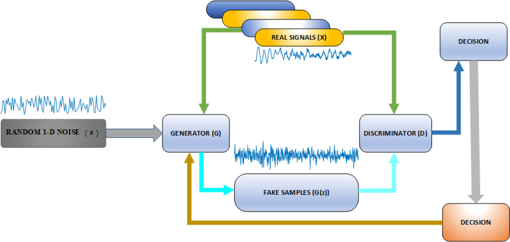
Figure 6 GAN architecture in general.

The function of generator G is to generate fake data to fool the discriminator as much as possible, while the discriminator D is trained to distinguish real data samples from synthesized samples. The input of the generator is a random noise vector z. The noise is mapped to a new data space through generator G to obtain a fake sample G(z), which is a multi-dimensional vector. Then, the discriminator D, which is a binary classifier, accepts either real data or fake data from generator G as an input and outputs the probability of the input being true and false. Then, the training process continues until the discriminator D cannot determine whether the data comes from the real dataset or from G. Finally, we obtained a model G, which can generate data that are similar to the real data. In prior work Ian et al. (2014), the discriminator D is defined as a binary classifier, whose loss function is represented by the cross entropy as follows:

$\begin{array}{ll}{J}^{(D)}=-\frac{1}{2}{\mathbb{E}}_{x\sim pdata}\log D(x)-\frac{1}{2}{\mathbb{E}}_z\text{log}(1-D(G(z))),& (3)\end{array}$

where x is the real sample, z is the random noise vector, G(z) are the data generated by the generator G, and E is the expectation. D(G(z)) indicates the probability that discriminator D determines the data are generated by G. The goal of D is for D(G(z)) to approach 0, while G aims to bring it closer to 1. Therefore, the loss of the generator can be derived via the discriminator D: f^(G)=-f^(D)

For the above reasons, the optimization problem of GANs is transformed into the minimax game as shown below:

$\begin{array}{ll}\underset{G}{\min }\underset{D}{\max }V(D,G)={\mathbb{E}}_{x\sim pdata}\log D(x)+{\mathbb{E}}_{z\sim p(z)}\log (1-D(G(z)))& (4)\end{array}$

The whole process of the algorithm is roughly as follows:

1. update the discriminator by ascending its stochastic gradient:

$\begin{array}{ll}\nabla {\theta }_d{\displaystyle \sum _{i=1}^m[\log D(x^{(i)})+log1-D(G(z^{(i)}))]}& (5)\end{array}$

2. Sample mini-batch of m noise samples z⁽¹⁾, z⁽²⁾, …,z^(m);

3. Update the generator by descending its stochastic gradient:

$\begin{array}{ll}\nabla {\theta }_d\frac{1}{m}{\displaystyle \sum _{i=1}^m+\log 1-D(G(z^{(i)}))}& (6)\end{array}$

These training sessions are then alternated until equilibrium is achieved.

The performance of the GAN is basically determined by its structure. Due to the deficiencies of the original GANs, various derived GANs models have been proposed. DCGAN Radford et al. (2015) is based on the use of a CNN; it is regarded as an effective network model of supervised learning, and is the most common generator and discriminator structure. The general two-dimensional convolution kernel is mainly used to process images, and it is difficult to directly process the one-dimensional ship-radiated noise signal. We use a one-dimensional convolution filter to fit ship-radiated noise. The structure is illustrated in Figure 7.

FIGURE 7

Figure 7 One-dimensional DCGAN architecture.

3.2 Generated sample results analysis

Due to the non-linear, non-Gaussian and non-stationary characteristics of ship-radiated noise, it is difficult to evaluate the quality of the generated data with traditional amplitude and frequency characteristics. We used the statistical distribution characteristics of the generated data, such as Mutual information (MI) and correlation coefficient (CC), to conduct a preliminary similarity analysis of the generated samples. MI is a measure of the degree of interdependence between variables:

$\begin{array}{ll}MI(X;Y){\displaystyle \sum _{y\in Y}{\displaystyle \sum _{x\in Y}p(x,y)\text{log}(\frac{p(x,y)}{p(x)p(y)})}}& (7)\end{array}$

We obtained MI between the generated samples and the original samples to measure the correlation between the samples. CC is the coefficient of correlation between different statistics:

$\begin{array}{ll}CC(X,Y)=\frac{\text{Cov}(X,Y)}{{\sigma }_x{\sigma }_y}& (8)\end{array}$

where Cov(X,Y) is the covariance, and σ is the standard deviation. Fifty pairs of samples are randomly selected from the original samples and the generated samples, and the average values of the MI and CC are calculated. The specific results are shown in Tables 2, 3.

TABLE 2

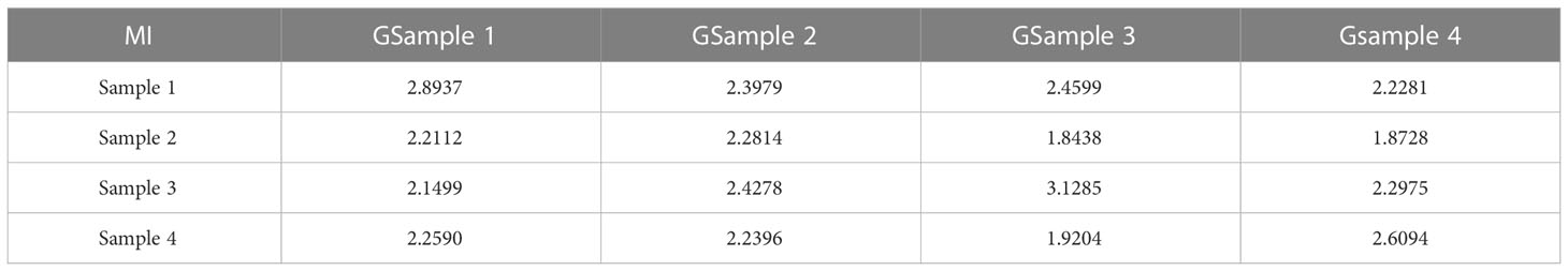
Table 2 Mutual information results.

TABLE 3

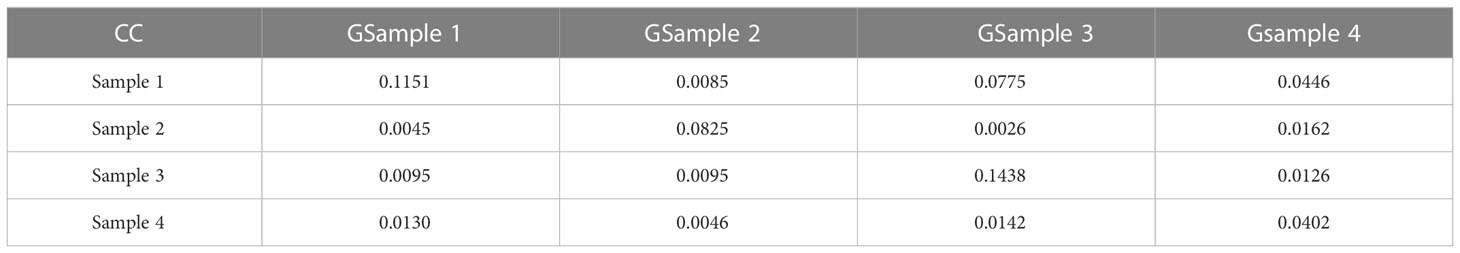
Table 3 Correlation coefficient results.

MI and CC are indices used to evaluate the similarity between two variables and for both indices, higher values correspond to a greater similarity between the variables. We see from the tables that MI and CC between samples of the same type, such as Sample 1 and Gsample 1, are higher than those between other samples. However, the gap between classes is not very obvious. To further verify the reliability of the generated samples, we used the DE, which is more suitable for nonlinear signal analysis, to compare the generated samples with the original samples. Similarly, we selected 50 samples of each kind and calculated the average value. The results are shown in Table 4.

TABLE 4

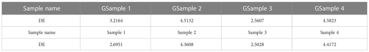
Table 4 Dispersion entropy results.

As shown in Table 4, the DE values of the generated samples of types 2, 3, and 4 are very close to the original samples, which indicates that the samples generated by GAN are consistent with the original samples, and there is diversity among samples. However, the DE values of type 2 and 4 are also relatively close, which is also one of the difficulties in the classification of ship-radiated noise. The DE values of type 1 had some gaps, but CC and MI performed better, and this also verifies the diversity of the generated samples. The generated samples could be therefore be used to form a new training dataset for training a ship-radiated noise classifier.

4 Classification based on deep learning

Given the connection between different network layers, deep neural networks extract signal features for classification inherently. Convolutional neural networks are a traditional type of deep neural network. Compared with SVMs, they require more data to ensure that the network will not be overfitted, but they perform better on unprocessed data. Deep networks with better performance have emerged with the continuous development of deep learning. ResNet He et al. (2015) uses direct mapping to connect different layers, solves the problem of gradient disappearance or gradient explosion problems, and greatly improves the model fitting capability than networks without this module. In this study, we used the sample length of 1,600 sampling points selected in Section 2 as the input size of the network for model construction, and the samples generated in Section 3 are used to mix with the original samples in different proportions to construct a new dataset as the training dataset of the network.

To observe the impact of generated samples on the final classification, we set up five training sets with different proportions of the original samples and the generated samples as follows: only 400 original samples, 400 original samples and 100 generated samples, 400 original samples and 200 generated samples, 400 original samples and 400 generated samples, and 400 original samples and 800 generated samples. The number of original samples in the test set is set according to the 10% ratio of the training set. The structure of the CNN is similar to the GAN discriminator, with the last dense classification layer changed to a layer using a four-way Softmax activation function, and the structure is shown in Figure 8. The parameters of three 1D-convolution layers are (64,3,2), (128,3,2), and (256,3,1). The first parameter is the number of convolution kernels; the second parameter is the kernel size; the last parameter is stride; and the value of padding is set to same, which means that it complements 0 uniformly during the sliding process of the convolution kernel. The parameter in the dense layer is set to (4,softmax), which means that the CNN used Softmax as the activation function for the four classifications. The structure of ResNet is shown in Figure 9. The parameters of the 1D-convolution layers before the residual modules are (64,3,1) and (64,3,1); the parameters of the 1D-convolution layer in the first batch of residual modules are (16,1,1), (16,3,1), and (64,1,1); and the parameters of the next 1D-convolution layer are (128,3,1). The parameters of the 1D-convolution layer in the first batch of residual modules are (32,1,1), (32,3,1), and (128,1,1). Then, the parameter of the first dense layer is (2048, relu), which means that the dimension of the output is 2,048, and the dense layer used the ReLU function as the activation function to fully connect the data. The parameter of the second dense layer is (4,softmax), and the function is same to the dense layer in CNN. The results are shown in Figures 10, 11.

FIGURE 8

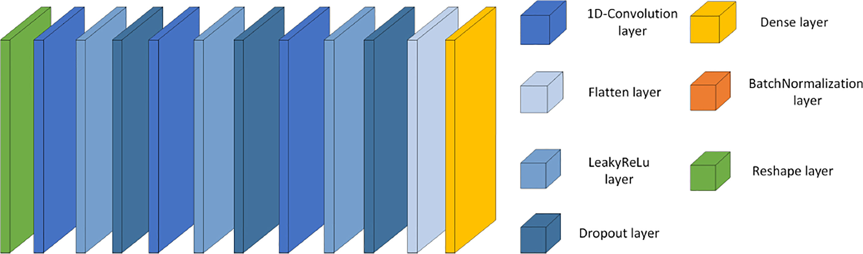
Figure 8 CNN structure.

FIGURE 9

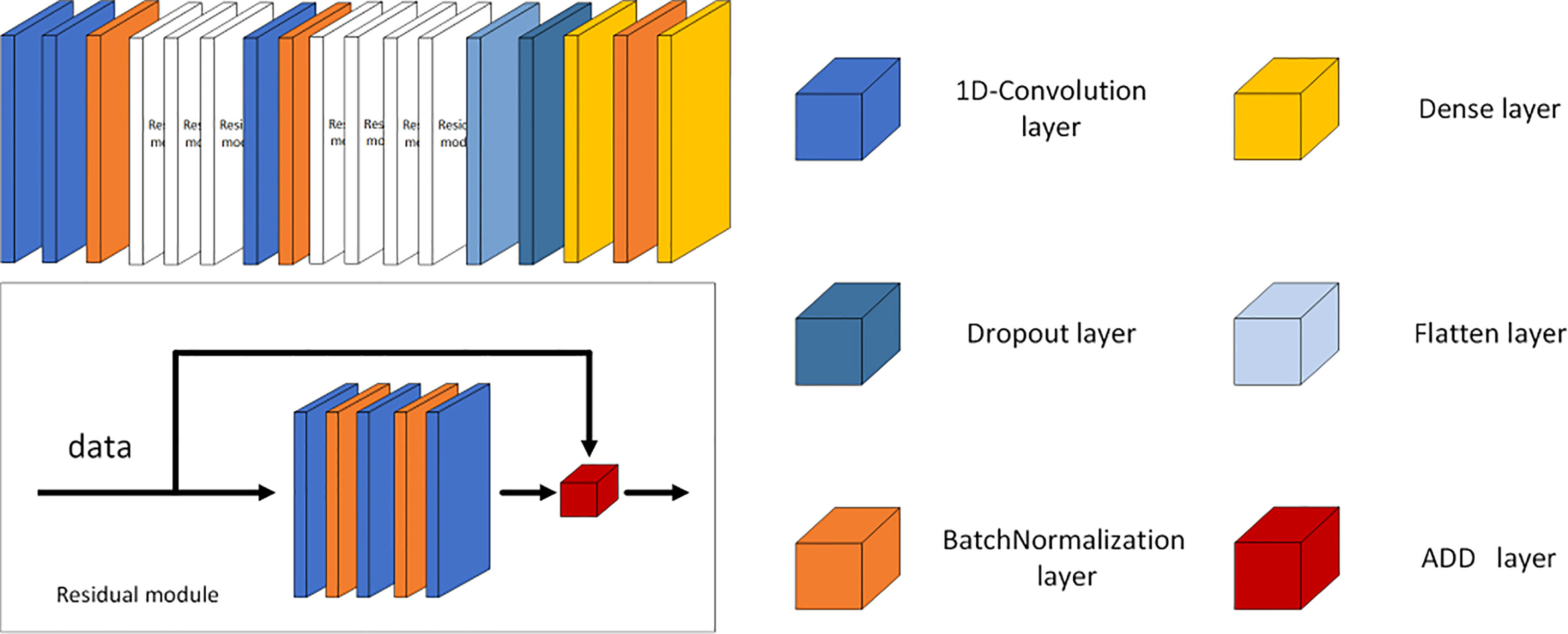
Figure 9 ResNet structure.

FIGURE 10

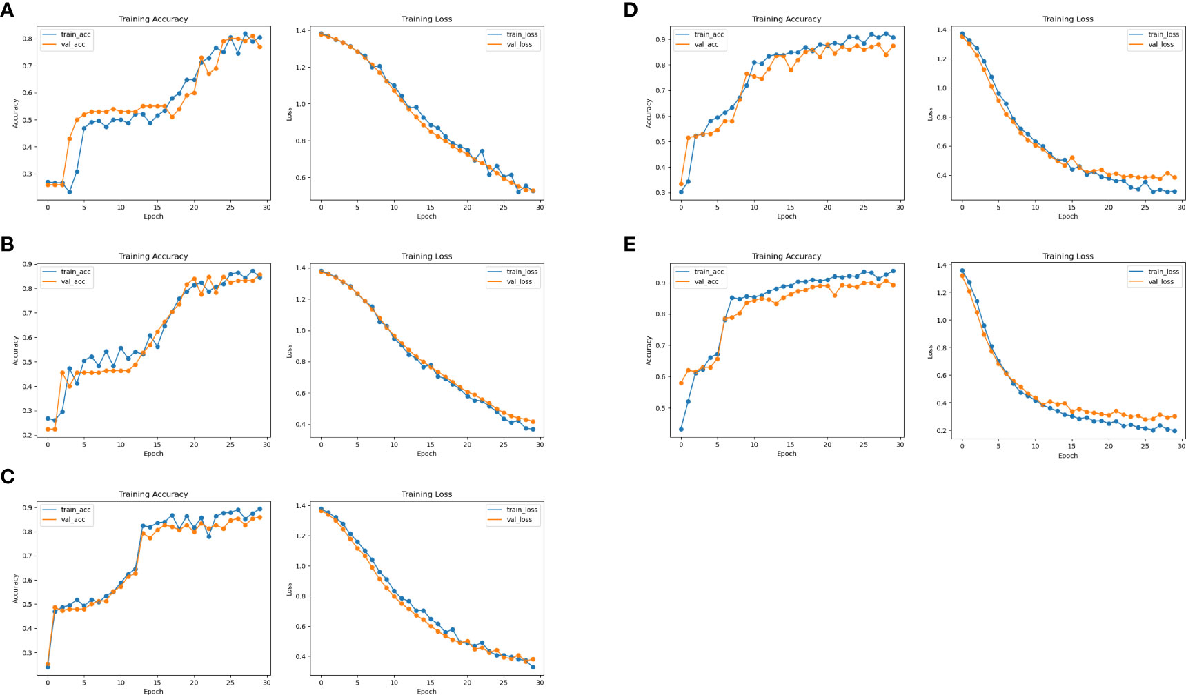
Figure 10 CNN classification results. (A) Results of the CNN on the original dataset. (B) Results of the CNN at 4:1 dataset. (C) Results of the CNN at 2:1 dataset. (D) Results of the CNN at 1:1 dataset. (E) Results of the CNN at 1:2 dataset.

FIGURE 11

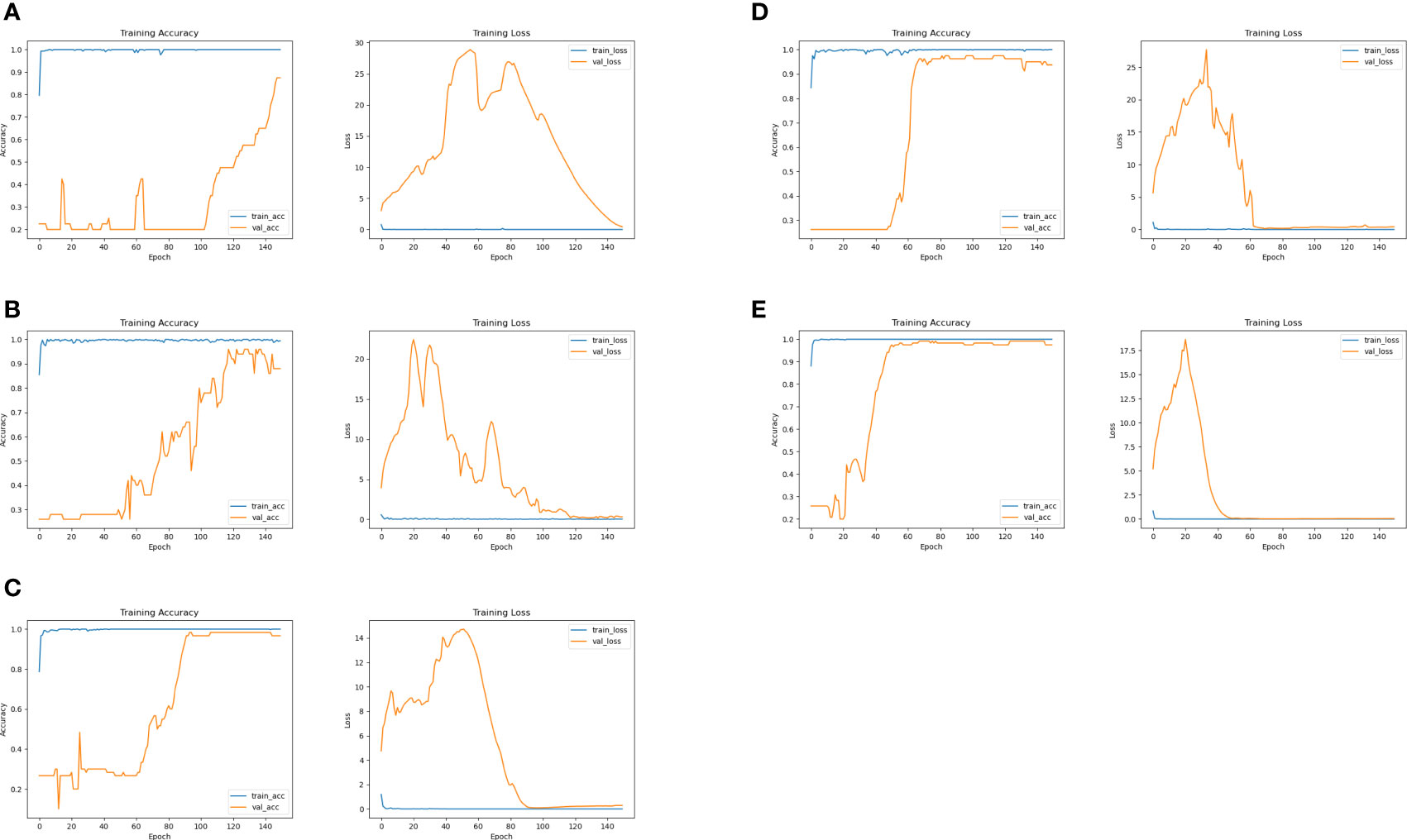
Figure 11 ResNet classification results. (A) Results of ResNet on the original dataset. (B) Results of ResNet at 4:1 dataset. (C) Results of ResNet at 2:1 dataset. (D) Results of ResNet at 1:1 dataset. (E) Results of ResNet at 1:2 dataset.

The images on the left are the training accuracy results, while the images on the right are the training loss results. Figures 10A and 11A show 400 original samples of 4 categories, including 100 samples in each category. They are then input into the traditional CNN and one-dimensional ResNet for classification.

The rest of the figures are the classification results obtained from the datasets formed when the ratio of original to generated samples is 4:1 in Figure 10B, 2:1 in Figure 10C, 1:1 in Figure 10D, and 1:2 in Figure 10E, respectively. In Figures 10, 11, the lines “train-acc” and “train-loss” are the results obtained in the training set, and “val-acc” and “val-loss” are the results obtained in the testing set.

The classification accuracy of the CNN using the dataset with only original samples is 79% in Figure 10A. When 100 generated samples are added to the dataset, the classification rate significantly improved, reaching 85.6% in Figure 10B. Adding another 100 generated samples to the dataset caused the classification accuracy to reach 86.68% in Figure 10C, with a 2:1 ratio of the original to generated samples. When the ratio is 1:1, the accuracy rose to 89.5% in Figure 10D. However, when the ratio is 1:2, the accuracy reached 90% in Figure 10E and did not increase significantly.

At this point, the sample size already met the requirements of the network structure, and the accuracy reached convergence, which also verifies the validity of the generated samples. ResNet has more network layers than a traditional CNN, and thus more training epochs are required. Therefore, the epoch number is set to 150. As shown in Figure 11, when we used the original dataset, the accuracy and loss converged slowly, and the accuracy only reached an eventual value of 87.5% in Figure 11A. As the number of samples increased, the accuracy gradually improved. After adding 100 samples into the dataset, the accuracy reached 92.5% in Figure 11B, but it is not stable and there are still some problems with overfitting.

Then, another 100 generated samples are added to the dataset, and the accuracy reached 98.33% in Figure 11C. The accuracy reached 97.5% in Figure 11D when the ratio of the original sample to the number of generated samples is 1:1. Finally, the accuracy reached 99.17% in Figure 11E when the ratio is 1:2. In the process of network model training and testing, each epoch took about 16 seconds. The number of epochs needed for convergence is reduced from 150 to 50 on testing set, and the convergence time is reduced from 40 minutes to 13.3 minutes. After network training is completed, when the new ship-radiated noise data are obtained, we only needed to perform sample segmentation and input them into the network directly without complex signal decomposition and manual feature extraction for classification. A classification result with an accuracy of 99% could be obtained within a few minutes.

5 Conclusion

In this paper, a 1-DDCGAN based on GAN is applied to extend ship-radiated noise under small sample size conditions. Deep neural network can extract sufficiently deep and essential features through the network structure when the sample size is large enough, and these features are used as a basis for classification. One-dimensional CNN and ResNet are designed for data analysis. And the accuracy is improved from 79% to 90% in CNN, from 87.5% to 99.17% in ResNet as the sample size increases.

Data availability statement

The original contributions presented in the study are included in the article/supplementary material. Further inquiries can be directed to the corresponding author.

Author contributions

ZX: Conceptualization, visualization, writing, project administration, original draft. RL: supervision, writing review. LW: supervision, writing review, editing. AZ: Supervision, conceptualization. JL: Writing review, editing. XT: Writing review, editing. All authors contributed to the article and approved the submitted version.

Funding

This work was supported by the Key Program of Marine Economy Development Special Foundation of Department of Natural Resources of Guangdong Province (GDNRC [2022]19), and Natural Resources Science and Technology Innovation Project of Fujian Province (KY-080000-04-2021-030).

Conflict of interest

Author XT was employed by Xiamen Weilai Marine Science and Technology Ltd.

The remaining authors declare that the research was conducted in the absence of any commercial or financial relationships that could be construed as a potential conflict of interest.

Publisher’s note

All claims expressed in this article are solely those of the authors and do not necessarily represent those of their affiliated organizations, or those of the publisher, the editors and the reviewers. Any product that may be evaluated in this article, or claim that may be made by its manufacturer, is not guaranteed or endorsed by the publisher.

References

Arniriparian S., Freitag M., Cummins N., Gerczuk M., Pugachevskiy S., Schuller B. (2018). “A fusion of deep convolutional generative adversarial networks and sequence to sequence autoencoders for acoustic scene classification,” in 2018 26th European signal processing conference (EUSIPCO) (Rome, Italy: IEEE), 977–981.

Google Scholar

Atanackovic L., Vakilian V., Wiebe D., Lampe L., Diamant R. (2020). “Stochastic ship-radiated noise modelling via generative adversarial networks,” in Global oceans 2020: Singapore–US gulf coast (Biloxi, MS, USA: IEEE), 1–8.

Google Scholar

Aziz W., Arif M. (2005). “Multiscale permutation entropy of physiological time series,” in 2005 Pakistan section multitopic conference (Karachi, Pakistan: IEEE), 1–6.

Google Scholar

Buda M., Maki A., Mazurowski M. A. (2018). A systematic study of the class imbalance problem in convolutional neural networks. Neural Networks 106, 249–259. doi: 10.1016/j.neunet.2018.07.011

PubMed Abstract | CrossRef Full Text | Google Scholar

Chen Z., Li Y., Cao R., Ali W., Yu J., Liang H. (2019). A new feature extraction method for ship-radiated noise based on improved ceemdan, normalized mutual information and multiscale improved permutation entropy. Entropy 21, 624. doi: 10.3390/e21060624

PubMed Abstract | CrossRef Full Text | Google Scholar

He K., Zhang X., Ren S., Sun J. (2015). Deep residual learning for image recognition. arXiv. doi: 10.48550/arXiv.1512.03385

CrossRef Full Text | Google Scholar

Ian G., Pouget-Abadie J., Mirza M., Xu B., Warde-Farley D. (2014). “Generative adversarial nets,” in Advances in neural information processing systems. arXiv. doi: 10.48550/arXiv.1406.2661

CrossRef Full Text | Google Scholar

Jiao S., Geng B., Li Y., Zhang Q., Wang Q. (2021). Fluctuation-based reverse dispersion entropy and its applications to signal classification. Appl. Acoust. 175, 107857. doi: 10.1016/j.apacoust.2020.107857

CrossRef Full Text | Google Scholar

Li Y., Geng B., Jiao S. (2022). Dispersion entropy-based lempel-ziv complexity: A new metric for signal analysis. Chaos Solitons Fractals 161, 112400. doi: 10.1016/j.chaos.2022.112400

CrossRef Full Text | Google Scholar

Li Y., Li Y., Chen X., Yu J. (2017). Denoising and feature extraction algorithms using npe combined with vmd and their applications in ship-radiated noise. Symmetry 9, 256. doi: 10.3390/sym9110256

CrossRef Full Text | Google Scholar

Li Y., Li Y., Chen X., Yu J., Yang H., Wang L. (2018). A new underwater acoustic signal denoising technique based on ceemdan, mutual information, permutation entropy, and wavelet threshold denoising. Entropy 20, 563. doi: 10.3390/e21010011

PubMed Abstract | CrossRef Full Text | Google Scholar

Li Z., Li Y., Zhang K. (2019). A feature extraction method of ship-radiated noise based on fluctuation-based dispersion entropy and intrinsic time-scale decomposition. Entropy 21, 693. doi: 10.3390/e21070693

PubMed Abstract | CrossRef Full Text | Google Scholar

Lin Z., Di C., Chen X., Hou Y. (2021). Acoustic recognition method in low snr based on human ear bionics. Appl. Acoust. 182, 108213. doi: 10.1016/j.apacoust.2021.108213

CrossRef Full Text | Google Scholar

Li J., Yang H. (2021). The underwater acoustic target timbre perception and recognition based on the auditory inspired deep convolutional neural network. Appl. Acoust. 182, 108210. doi: 10.1016/j.apacoust.2021.108210

CrossRef Full Text | Google Scholar

Noda J. J., Travieso-González C. M., Sánchez-Rodríguez D., Alonso-Hernández J. B. (2019). Acoustic classification of singing insects based on mfcc/lfcc fusion. Appl. Sci. 9, 4097. doi: 10.3390/app9194097

CrossRef Full Text | Google Scholar

Pan Z., Yu W., Yi X., Khan A., Yuan F., Zheng Y. (2019). “Recent progress on generative adversarial networks (gans): A survey,” in IEEE Access, Vol. 7. 36322–36333. doi: 10.1109/ACCESS.2019.2905015

CrossRef Full Text | Google Scholar

Pethiyagoda R., Moroney T. J., Macfarlane G. J., Binns J. R., McCue S. W. (2018). Time-frequency analysis of ship wave patterns in shallow water: modelling and experiments. Ocean Eng. 158, 123–131. doi: 10.1016/j.oceaneng.2018.01.108

CrossRef Full Text | Google Scholar

Qi J., Yang H., Sun H. (2020). “Mod-rrt*: A sampling-based algorithm for robot path planning in dynamic environment,” in IEEE Transactions on Industrial Electronics, Vol. 68. 7244–7251. doi: 10.1109/TIE.2020.2998740

CrossRef Full Text | Google Scholar

Radford A., Metz L., Chintala S. (2015). Unsupervised representation learning with deep convolutional generative adversarial networks. arXiv. doi: 10.48550/arXiv.1511.06434

CrossRef Full Text | Google Scholar

Richman J. S., Lake D. E., Moorman J. R. (2004). “). sample entropy,” in Methods in enzymology, vol. 384. (Cambridge, MA, USA: Academic Press), 172–184. doi: 10.1016/S0076-6879(04)84011-4

CrossRef Full Text | Google Scholar

Santos-Domínguez D., Torres-Guijarro S., Cardenal-López A., Pena-Gimenez A. (2016). Shipsear: An underwater vessel noise database. Appl. Acoust. 113, 64–69. doi: 10.1016/j.apacoust.2016.06.008

CrossRef Full Text | Google Scholar

Shi Y., Li B., Du G., Dai W. (2021). Clustering framework based on multi-scale analysis of intraday financial time series. Physica A: Stat. Mechan. its Appl. 567, 125728. doi: 10.1016/j.physa.2020.125728

CrossRef Full Text | Google Scholar

Wei X. (2016). “On feature extraction of ship radiated noise using 11/2 d spectrum and principal components analysis,” in 2016 IEEE international conference on signal processing, communications and computing (ICSPCC) (Hong Kong, China: IEEE), 1–4.

Google Scholar

Xie D., Esmaiel H., Sun H., Qi J., Qasem Z. A. H. (2020). Feature extraction of ship-radiated noise based on enhanced variational mode decomposition, normalized correlation coefficient and permutation entropy. Entropy 22, 468. doi: 10.3390/e22040468

PubMed Abstract | CrossRef Full Text | Google Scholar

Yang H., Cheng Y., Li G. (2021). A denoising method for ship radiated noise based on spearman variational mode decomposition, spatial-dependence recurrence sample entropy, improved wavelet threshold denoising, and savitzky-golay filter. Alexandria Eng. J. 60, 3379–3400. doi: 10.1016/j.aej.2021.01.055

CrossRef Full Text | Google Scholar

Yan X., Song H., Peng Z., Kong H., Cheng Y., Han L. (2021). Review of research results concerning the modelling of shipping noise. Polish Maritime Res. doi: 10.2478/pomr-2021-0027

CrossRef Full Text | Google Scholar

Zhang H., Junejo N. U. R., Sun W., Chen H., Yan J. (2020a). “Adaptive variational mode time-frequency analysis of ship radiated noise,” in 2020 7th international conference on information science and control engineering (ICISCE) (Changsha, China: IEEE), 1652–1656.

Google Scholar

Zhang X., Wu H., Sun H., Ying W. (2021). Multireceiver sas imagery based on monostatic conversion. IEEE J. Selected Topics Appl. Earth Observat. Remote Sens. 14, 10835–10853.

Google Scholar

Zhang W., Wu Y., Wang D., Wang Y., Wang Y., Zhang L. (2018). “Underwater target feature extraction and classification based on gammatone filter and machine learning,” in 2018 international conference on wavelet analysis and pattern recognition (ICWAPR) (Chengdu, China: IEEE), 42–47.

Google Scholar

Zhang X., Yang P. (2022). Back projection algorithm for multi-receiver synthetic aperture sonar based on two interpolators. J. Mar. Sci. Eng. 10, 718. doi: 10.3390/jmse10060718

CrossRef Full Text | Google Scholar

Zhang X., Yang P., Feng X., Sun H. (2022a). Efficient imaging method for multireceiver sas. IET Radar Sonar Navigat.

Google Scholar

Zhang X., Yang P., Sun H. (2022b). Frequency-domain multireceiver synthetic aperture sonar imagery with chebyshev polynomials. Electron. Lett.

Google Scholar

Zhang X., Yang P., Sun M. (2022c). Experiment results of a novel sub-bottom profiler using synthetic aperture technique. Curr. Sci. (00113891) 122, 461–464.

Google Scholar

Zhang X., Ying W., Yang P., Sun M. (2020b). Parameter estimation of underwater impulsive noise with the class b model. IET Radar Sonar Navigat. 14, 1055–1060.

Google Scholar