Reconstruction of horizontal tidal current fields in a shallow water with model-oriented coastal acoustic tomography

Reciprocal acoustic transmission and coastal acoustic tomography (CAT) is a powerful tool for measuring tidal currents in shallow coastal water, especially if data assimilation is employed. In previous CAT data assimilation studies, the ensemble Kalman filter (EnKF) has been implemented to assimilate observed path-averaged velocity, but ad-hoc procedures called localization and inflation, which compensate for issues associated with using ensemble approximation, were not always implemented. In this study, EnKF is applied to assimilate the path-averaged currents obtained from a reciprocal acoustic transmission experiment conducted at Mihara-Seto in the Seto Inland Sea, Japan, with four acoustic stations in 2020 to reconstruct spatiotemporal variations of tidal currents at the observation site. We executed EnKF with several combinations of different values of the inflation, localization, and the number of ensemble members. The resulting data assimilated velocity reconstructions are compared with acoustic Doppler current profiling (ADCP) results. The results show that data assimilation with EnKF improved the velocity reproduction compared with the model prediction and that implementing covariance inflation contributed to additional improvements. The covariance localization did not improve the results in our case. The best result in terms of fractional error variance (FEV) between the ADCP velocity was obtained from the case with 980 ensemble members with a covariance inflation of 1.01; the FEV was 7.9%. The case of 98 ensemble members with a covariance inflation of 1.01 resulted in similar performance; the FEV value was 8.2%. Thus, with the covariance inflation, the number of ensemble member used in previous CAT studies are reasonable. In the study, we also clarified the reason for the high-frequency variation in the observed path-averaged currents in a preliminary experiment; the path-averaged currents had captured the spatiotemporal variation of vortex generation associated with island wakes. The reciprocal acoustic transmission with EnKF can capture short-period variation over a long period; thus, it can be used in studies of coastal physical processes with various time scales.

1 Introduction

Ocean acoustic tomography (OAT) is a unique method of acoustical oceanography for remotely sensing the sound speed and current in the ocean interior (Munk and Wunsch, 1979; Munk et al., 1995). In OAT, one transmits and receives acoustic signals between multiple sources/receivers through the ocean, precisely determines travel times of acoustic signals, and then, applies an inverse method to the determined travel times to estimate the ocean interior states (sound speed and ocean currents) traversed by the acoustic paths. The effects of sound speed and ocean currents on the travel times can be separated by computing the sum and difference of the travel times obtained from reciprocal acoustic transmission. This OAT and reciprocal acoustic transmission methods have been applied to coastal shallow water, which may be referred to as coastal acoustic tomography (CAT). Readers can refer to Kaneko et al. (2020) and references therein for the application of reciprocal acoustic transmission (and CAT) in shallow water around Japan. Because of its usefulness, the concept of OAT and reciprocal acoustic transmission have further been applied to a very small port (e.g., Ogasawara and Mori, 2016) and/or rivers (e.g., Kawanisi et al., 2017). Additionally, multiple new approaches have been proposed, such as deploying networked array (Huang et al., 2013; Chen et al., 2021), moving ship tomography (Huang et al., 2019) originating from the work by Cornuelle et al. (1989), or physics based approach (Wang et al., 2018).

A promising method of OAT/CAT is a model-oriented inverse method (state estimation or data assimilation; Munk et al., 1995). Data method assimilation have now been widely used in science and engineering fields and there are multiple assimilation schemes (e.g., Evensen, 2009, and references therein). Among various assimilation schemes, the data assimilation with ensemble Kalman filter (EnKF; Evensen, 1994) is ease to implement yet powerful enough to reproduce tidal currents in shallow water by assimilating the reciprocal acoustic transmission data (Park and Kaneko, 2000; Lin et al., 2005). The CAT with EnKF data assimilation have been used to discuss physical process in coastal seas (Zhu et al., 2017; Chen et al., 2017; Zhu et al., 2021). Recently, CAT data assimilation is implemented with velocity fields obtained from an ocean radar observation (Zhu et al., 2022).

EnKF approximates model covariance by ensemble covariance, which enables the application of Kalman filter theory to nonlinear models (like a nonlinear numerical ocean model) and large state dimensions. However, approximating model covariance by ensemble covariance with a finite ensemble size causes several issues, such as long-range spurious or unphysical correlations in covariances (sampling error) and the underestimation of the ensemble variance. Thus, EnKF implementation requires somewhat ad-hoc tuning such as localization and inflation (e.g., Evensen, 2009). The common approach of localization is covariance localization, which damps long-range spurious correlation and localize the effect of data assimilation near the observation location (e.g., Hamill et al., 2001). The inflation is to broaden the updated analysis in order to counteract the excessive variance reduction caused by spurious correlations in the update (e.g., Anderson and Anderson, 1999).

The above mentioned localization and inflation have not been implemented commonly in CAT data assimilation studies. An advantage of CAT method in coastal shallow sea is that path-averaged currents can be measured and assimilated into ocean models with a short time interval (e.g., every few minutes). However, frequent Kalman filter updates with an underestimated ensemble variance (due to small ensemble sizes) leads to filter divergence. Filter divergence might happen in previous CAT studies. For example, there was a case that ensemble spreads of predicted path-averaged currents over some paths were not large enough for some period, and analysis steps of assimilation did not improve effectively (e.g., Figure 11 in Zhu et al., 2017). Therefore, it seems that the covariance inflation has possibility to improve the CAT data assimilation with EnKF, in particular when the path-averaged currents are assimilated frequently. An example of the use of covariance localization is that by Chen et al. (2017), which implemented the covariance localization to the problem of upwelling associated with typhoon passage (with relatively strong wind). On the one hand, tidal currents will be spatially correlated in a small study area, and covariance localization may not be required; on the other hand, if EnKF is used with small ensemble members, there will arise spurious correlation and localization may be required. Chen et al. (2017) implemented the covariance localization, but improvements associated with the localization is not clear.

We conducted a reciprocal acoustic transmission experiment between a pair of transceivers (i.e., acoustic stations) deployed in an area of complex coastlines with multiple islands and channels around Mihara-Seto in the Seto Inland Sea, Japan (Figure 1) in 2019 and demonstrated the capability of reciprocal acoustic transmission to capture high frequency variations of small magnitude in tidal currents (Taniguchi et al., 2021a). In 2020, we conducted a reciprocal acoustic transmission experiment using four acoustic stations deployed at the same observation site to determine the capability of data assimilation with reciprocal acoustic transmission to reproduce complex current velocity fields in the observation site. We developed a numerical ocean model for simulating depth-averaged flow around the observation site (i.e., two dimensional model) and applied EnKF to assimilating the path-averaged currents to the numerical ocean model.

FIGURE 1

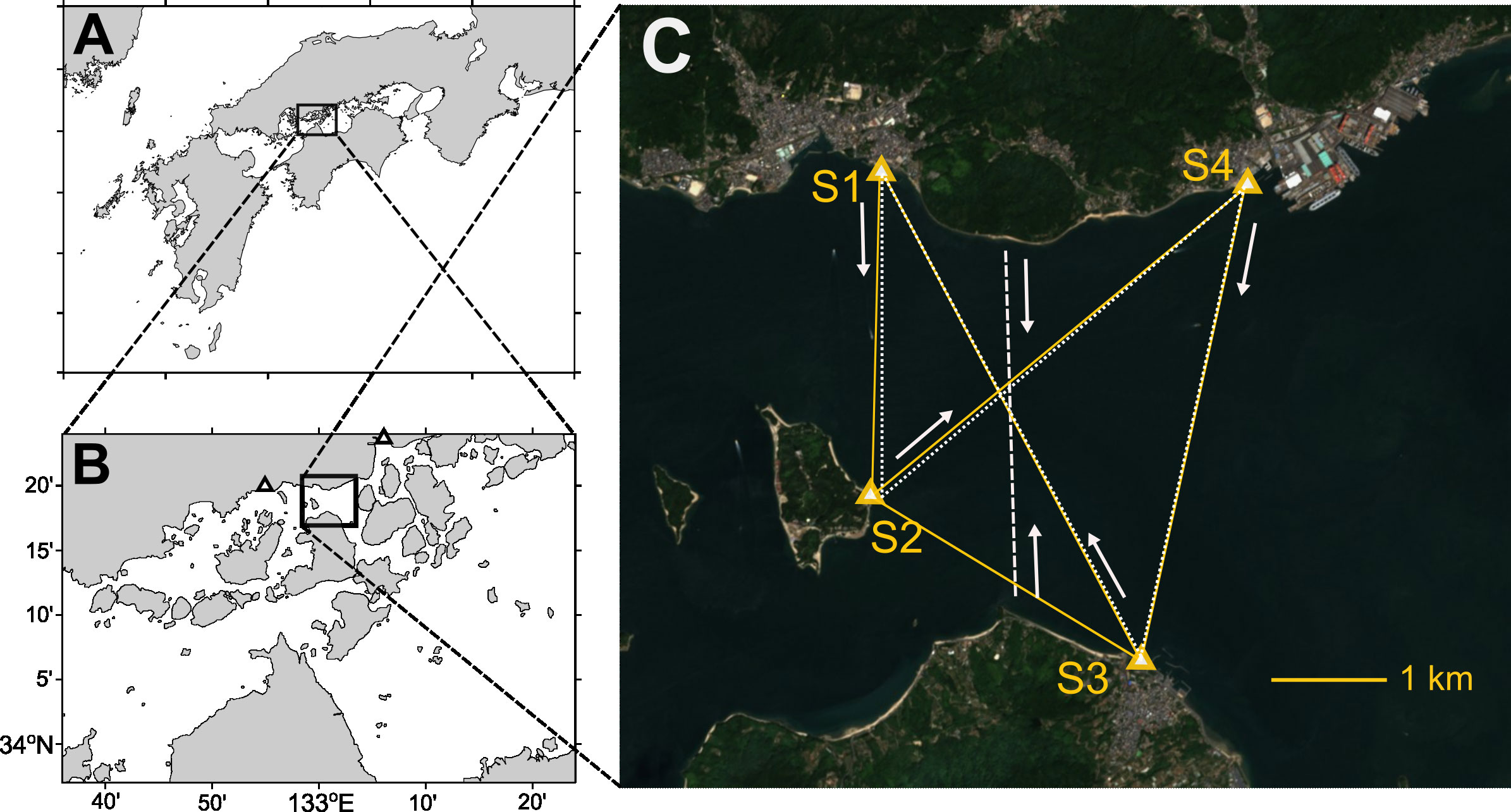
Figure 1 (A, B) Geographical location of observation site (Mihara-Seto) in the Seto Inland Sea, Japan; (C) satellite (Sentinel-2) image of observation site and locations of acoustic stations (four triangles with labels S1, S2, S3, and S4). The two black triangles in panel (B) is the location where astronomical tide information is obtained: Takehara for the west and Itozaki for the east. In panel (C), the five yellow lines are the acoustic transmission paths over each station pair; the white dashed and dotted lines indicate the tracks of shipboard acoustic Doppler current profiling (ADCP) observation performed on Oct. 30 and 31, respectively, with the arrows for the route direction.

The specific purpose of this paper is twofold. First, we clarify the performances of EnKF with path averaged currents in regard to the tuning parameters of covariance localization and covariance inflation as well as the number of ensemble members. We executed the sequential data assimilation of EnKF with several combinations for these values and compared the resulting velocity fields with the velocity from acoustic Doppler current profiling (ADCP) observation. Clarified results for the method performance can be a guidance for parameter choices and contribute to future study using the same method. The second purpose is to clarify the reasons for high-frequency variation found in the path-averaged currents in the preliminary experiment (Taniguchi et al., 2021a). Reciprocal acoustic transmission can be performed over a long period (or operationally) with sufficiently short time intervals. Although the data with short time interval may not contribute directory to reproducing spatially precise velocity field of tidal currents, the estimation can be precise for both spatially and temporally by combining with a numerical ocean model (thus, data assimilation method). As we shall see, the data assimilation results reveals that the path-averaged current had captured vortex generation behind an island (i.e., island wake). Such capability to reproduce the transient vortexes can advance the studies on physical processes on coastal shallow water.

2 Materials and methods

2.1 Field observation

An experiment on reciprocal acoustic transmission between four acoustic stations was conducted in a complex sea area of Mihara-Seto with multiple islands and channels from the end of October to December 2020. Figure 1 shows the geographical location of the observation site and the locations of the four acoustic stations (S1, S2, S3, and S4). The coast blocks the transmission between the S1 and S4 stations, and thus the travel time is not observable between them. The distances between the five station pairs (S1 and S2, S1 and S3, S2 and S3, S2 and S4, and S3 and S4) were 2842, 4895, 2805, 4300, and 4280 m, respectively. The travel-time measurement system used for this experiment was nearly the same as that used in a preliminary experiment in the same area in 2019 (Taniguchi et al., 2021a), which was initially developed for a moving-ship tomography study (Huang et al., 2019), with some changes and modifications. For this experiment, we used an electroacoustic transducer Model T235 (which can operate over a frequency band of 10–25 kHz) of Neptune Sonar as a transceiver. The ways of deploying the transceivers for stations S1 and S2 were the same as those in the preliminary experiment (Taniguchi et al., 2021a). The deployment of the S3 station was identical to that of the S1 station. For station S4, the transceiver was deployed about 1 m ahead of a pier using iron flames because there was rubble right next to the pier.

The reciprocal acoustic transmissions between the four stations were performed repeatedly every two minutes. A pulse compression method was implemented to increase the signal-to-noise ratio (SNR) without decreasing the time resolution. The transmitted signal in the experiment was a binary phase-shift keyed signal encoded by a pseudo-random binary sequence called a maximal length sequence (often referred to as an m-sequence).

Table 1 summarizes the transmission signal parameters for this experiment. In the experiment, we introduced two ideas on signal transmission (Taniguchi et al., 2021b). The first idea was about the periodicity of m-sequences: the transmission signal in the experiment was one period of an m-sequence of 2,047 digits (i.e., 11th order m-sequence; Table 1), but the last 63 and first 64 digits of the m-sequence were respectively added to the head and tail of the m-sequence to achieve the original auto-correlation property of repeated m-sequences. The other idea is about the transmission timing of the signal: the start time of each pulse was synchronized among all stations by using the one pulse-per-second signal of GPS, but time-shifted slightly so that the arrival signals do not overlap at all stations. Some of the results of the experiment are found in a report by Taniguchi et al. (2021b).

TABLE 1

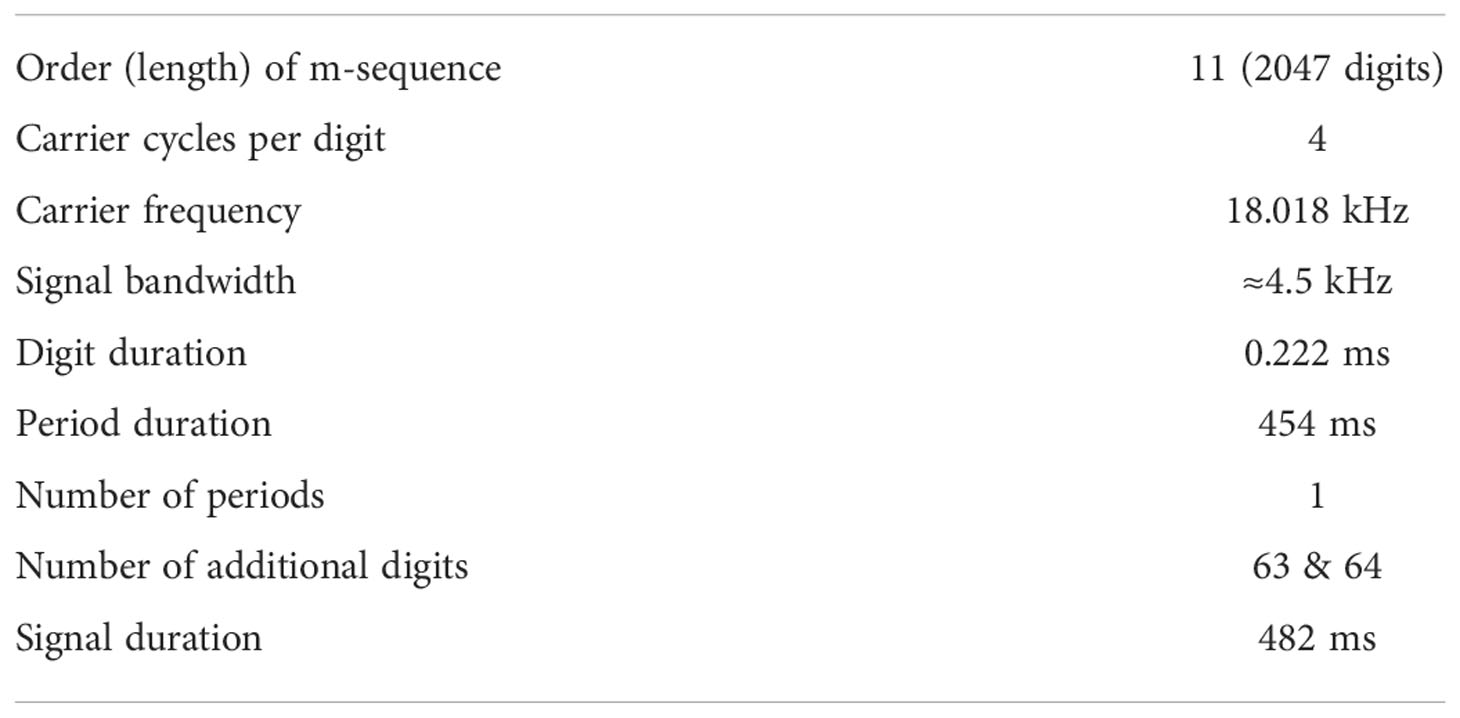
Table 1 Transmission signal parameters.

Travel times of acoustic signals were determined by detecting the time at which the received arrival pattern (i.e., the impulse response or cross-correlogram) first exceeded 14 dB. For each paired reciprocal acoustic transmission, differential travel times (τ_d) were computed from the determined travel times and converted to path-averaged current (u) as follows (Worcester, 1977; Howe et al., 1987; Zheng et al., 1997):

$\begin{array}{ll}u=\frac{c_0^2}{2L}{\tau }_d& (1)\end{array}$

where c₀ is the reference sound speed value, and L is the transceiver-to-transceiver distances. Here we assumed straight acoustic ray paths because the range-to-depth ratio is about 100:1, and the acoustic ray paths are nearly horizontal. Also, since the transceivers were nearly fixed in the experiment, the transceiver motion was not required to consider. The erroneous estimates of the path-averaged velocity were removed and linearly interpolated if the data gaps were less than 10 minutes. The obtained currents are path-averaged values but can be regarded as section-averaged currents because the tidal currents at the observation site are almost vertically uniform, as shown by an ADCP observation in the preliminary experiments (Taniguchi et al., 2021a). The path-averaged currents for each station pair were summarized as time series data starting from 16:00 on October 28, 2020. These time series of path-averaged (section-averaged) currents of the five station-pair were the data assimilated into a numerical ocean model.

We conducted shipboard ADCP observations on October 30 and 31 to obtain velocity data for comparison with data assimilation results. The ADCP used in the experiment was a WH-ADCP (Teledyne RD Instruments, Inc.). The details of the operating parameters for the ADCP observations are summarized in Table 2. The shipboard ADCP observations were made hourly from 07:00 to 17:00 along the north-south section on October 30 (dashed line in Figure 1C) and from 07:00 to 16:00 along the acoustic transmission lines (without the line connecting the S2 and S3 stations) on October 31 (dotted lines in Figure 1C). The fishing boat that had the ADCP installed traveled along each transect at an average ship speed of about 3–4 knots, taking about 20–45 min to complete the journeys. The ship track and speed were recorded using a differential GPS, which was used to correct the ADCP’s compass error (Trump and Marmorino, 1997). When the ship approached the S2 station, we allowed the ADCP’s transect to deviate from that of the acoustic transmission path for safety reasons because the location for the S2 station was continually used by ferry boats for passengers. In all, 21 cross-sections of velocity data were obtained along the north-south transect and along the transmission lines from these ADCP observations. After the shipboard ADCP observation, the recorded ADCP velocity data with the compass correction were averaged over the depth and then spatially (horizontally) averaged over about 100 m so that the spatial resolution of the ADCP velocity data is nearly the same as that of a numerical ocean model used in the data assimilation (see Sec. 2.2). This spatial average also corresponds to the time average over about 30 s.

TABLE 2

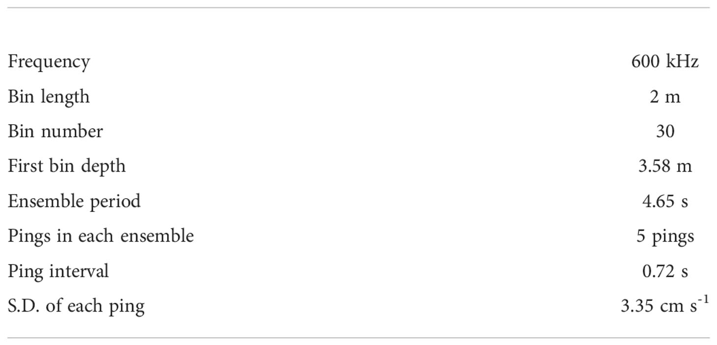
Table 2 ADCP operation parameters.

2.2 Numerical ocean model

A numerical ocean model used in this study is based on the depth-averaged shallow water equations of the following forms:

$\begin{array}{ll}\frac{\partial \eta }{\partial t}+\frac{\partial UD}{\partial x}+\frac{\partial VD}{\partial y}=0,& (2)\end{array}$

$\begin{array}{ll}\frac{\partial UD}{\partial t}+\frac{\partial U^{2}D}{\partial x}+\frac{\partial UVD}{\partial y}-fVD=-gD\frac{\partial \eta }{\partial x}+F_x-C_D\sqrt{U^2+V^2}U,& (3)\end{array}$

$\begin{array}{ll}\frac{\partial VD}{\partial t}+\frac{\partial UVD}{\partial x}+\frac{\partial V^{2}D}{\partial y}+fUD=-gD\frac{\partial \eta }{\partial y}+F_y-C_D\sqrt{U^2+V^2}V,& (4)\end{array}$

where (x,y) are the east-west and north-south coodinates; (U,V) are the eastward and northward components of the depth-averaged velocity; η is the free surface elevation; H is the water depth at rest; D is the total water depth (thus, D=H+η); f is the Coriolis parameter; g is the gravitational acceleration. The terms F_x and F_y are the lateral eddy viscosity and are defined according to

$\begin{array}{ll}{F}_x=\frac{\partial }{\partial x}\left(2H{A}_H\frac{\partial U}{\partial x}\right)+\frac{\partial }{\partial y}\left[H{A}_H\right(\frac{\partial U}{\partial y}+\frac{\partial V}{\partial x}\left)\right],& (5)\end{array}$

$\begin{array}{ll}{F}_y=\frac{\partial }{\partial y}\left(2H{A}_H\frac{\partial V}{\partial y}\right)+\frac{\partial }{\partial x}\left[H{A}_H\right(\frac{\partial U}{\partial y}+\frac{\partial V}{\partial x}\left)\right],& (6)\end{array}$

where A_H is the lateral kinematic eddy viscosity coefficient and was assigned a constant value of 4.8 m s^-2 in the present model. The last term in Eqs. (3) and (4) are the bottom stress, and the bottom drag coefficient C_D is given by the larger of the two values between 0.0025 and gn²/H^4/3 with Manning’s roughness coefficient n=0.0029.

The above shallow water equations are solved numerically using the finite difference method. The model domain is shown in Figure 2. The numerical discretization and integration schemes followed those used in Princeton Ocean Model (POM; Blumberg and Mellor, 1987). The grid space is 100 m. The time integration with a time step of 1 s was performed using a leap-frog scheme with a Robert-Asselin filter with an additional modification proposed by Williams (2009).

FIGURE 2

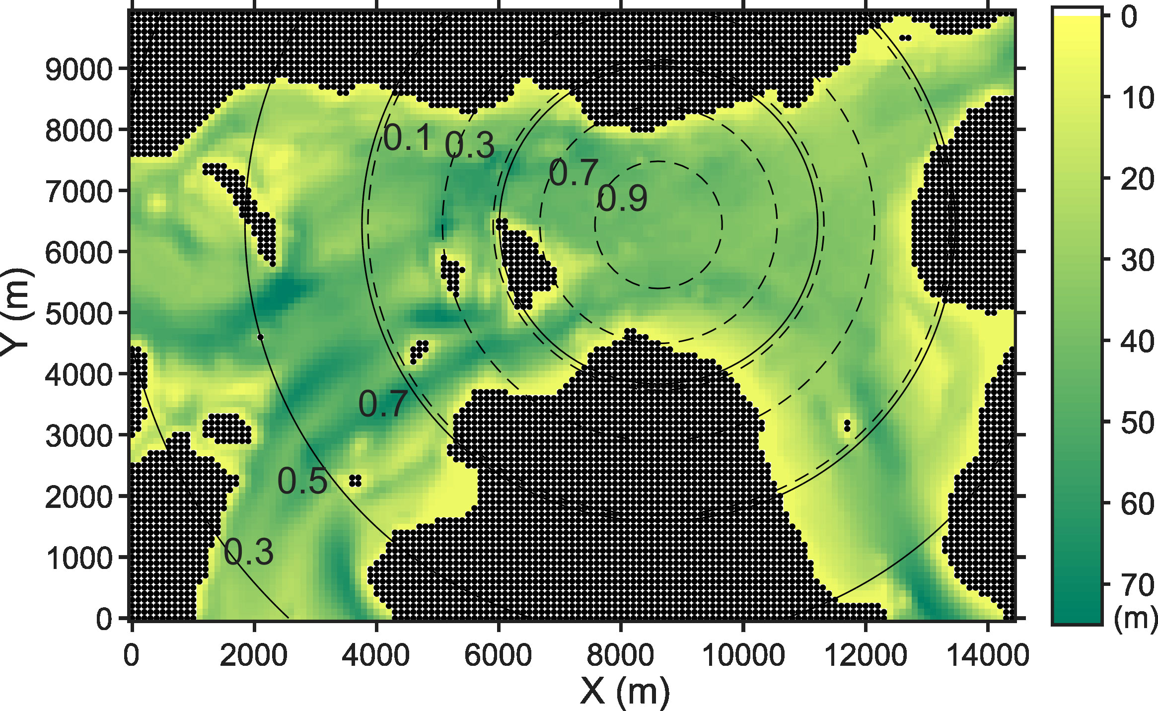
Figure 2 Domain of a numerical ocean model used in this study. The color indicates the water depth, and black dots correspond to land grids. The boundaries without dots (i.e., not land) are open boundaries where prescribed tidal forcing is given to drive the flow in the model domain. The dashed and solid circles are contours of the two covariance localization radii (4 km and 10 km) with a contour interval of 0.2.

The present model has six open boundaries (two at the west, east, and south). Tidal forcing at each open boundary drives the model interior. In the present model, a Flather condition, which is an extension of a radiation boundary condition, was implemented in the following way (e.g., Carter and Merrifield, 2007):

$\begin{array}{ll}{U}_{n,b}=U_n^{ext}\pm \sqrt{\frac{g}{H}}({\eta }_{b\pm 1}-{\eta }^{ext}),& (7)\end{array}$

where the subscripts n,b indicate the velocity normal to the boundary at the boundary grids; the superscript ext indicates using externally prescribed values. This Flather condition is less sensitive to errors in the prescribed boundary values compared with other boundary conditions, such as clamped surface elevations (Carter and Merrifield, 2007). The above Flather condition is provided for U at the west and east boundaries and V at the southern boundaries. The tidal elevations and normal velocities were constant along each open boundary in the present model. The tangential velocities at the boundary grids were given by the values of neighboring interior grids (i.e., a zero-gradient condition).

The prescribed tidal elevations at the west and east boundaries were derived from astronomical tides, i.e., the amplitudes and phases of five constituents (namely, M2, S2, K1, O1, and N2) at the nearest tide stations: Takehara for the west and Itozaki for the east (Figure 1B). These prescribed tidal elevations at the west and east boundaries are shown in Figure 3. There is no tide station near the two southern boundaries. Thus, the tidal elevations at the southwestern and southeastern boundaries were given by the same tidal elevations as the western and eastern boundaries, respectively. The tidal currents normal to the open boundaries were determined by using the information on path-averaged current via an ad-hoc way as follows. First, we applied a harmonic analysis to the path-averaged current observed between the S1 and S3 stations and estimated the amplitudes and phases of each tidal constituent at the observation site. The estimated phases for each tidal constituent were used to prescribe the normal velocity at the open boundaries. Second, we obtained the maximum tidal current at the east boundary as about 2.8 m s^-1 from a nautical chart (not shown here). This maximum current speed was multiplied by 0.8 to convert it to section averaged current speed, resulting in a maximum section-averaged current of 2.2 m s^-1. Third, the amplitudes of the estimated five tidal constituents for the normal velocity at the east boundary were scaled so that the reconstructed tidal currents by the five constituents reached 2.2 m s^-1 at the maximum during a spring tide. Then, amplitudes of the five constituents at other western and southern boundaries were determined so that the volume transport through these boundaries without the tidal elevations equal to that at eastern boundaries.

FIGURE 3

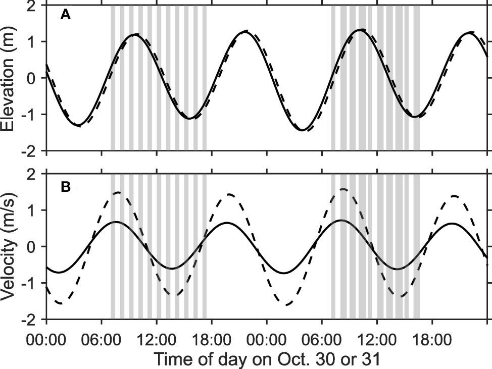
Figure 3 Time series of (A) tidal elevations and (B) tidal currents that were given as the open boundary conditions at the west (solid) and east (dashed) boundaries. The gray vertical bars indicate the time of the shipboard ADCP observation.

2.3 Data assimilation

As is the case with previous CAT data assimilation studies (Park and Kaneko, 2000; Lin et al., 2005; Zhu et al., 2017), the EnKF scheme (Evensen, 1994; Evensen, 2003; Evensen, 2009) accompanied Monte Carlo method is used to assimilate the path-averaged current data into the ocean model. In the present numerical ocean model, state variables are the east-west and north-south components of the depth-averaged velocity (U(x,y), V(x,y)) and sea surface elevation (tidal elevation; η). These state variables on all model grids are aligned and expressed as model state vector x_k where subscript k indicates the state vector at time k. The ocean model updates the model state vector x according to the governing equations and implemented numerical scheme. The relationship between the observed path-averaged current at time k and the model state vector x_k can be described as:

$\begin{array}{ll}{\mathit{y}}_k=\mathit{H}{\mathit{x}}_k+{\mathit{v}}_k,& (8)\end{array}$

where vector y_k contain the five path-averaged currents. Note that the observed path-averaged current cannot be assigned to a specific time step k of the model time step (1 s in the present model) because the acoustic signal travels and samples the ocean over a few seconds; thus, we assumed that the observed path-averaged currents are obtained at the scheduled time for each transmission (e.g., 00:00:00, 00:02:00, 00:04:00, and so on). The observation matrix H maps the model space (i.e., velocity fields) into observed space (i.e., path-averaged currents) and corresponds to the procedure that interpolates (U(x,y), V(x,y)) along the transmission paths, projects it onto the direction parallel to the paths, and averages over the paths. In practical computation, we did not define (or use) observation matrix H but computed Hx_k by interpolating, projecting, and path-averaging the velocity field at time k. The term v_k is observation noise and is assumed to be Gaussian noise with covariance R_k. The path-averaged currents are assumed to be independent over the station pairs, and thus, R_k is a diagonal matrix. We also assumed constant R_k over time in this study; thus, R_k=R. Considering the results of the preliminary experiment (Taniguchi et al., 2021a), we assigned 0.025² m² s^-2 for all the diagonal elements.

We assume here that the observed path-averaged currents are available at time k. The numerical ocean model predicts x_k of each N ensemble member to apply EnKF. The N state vectors x_k corresponding to N ensemble members forms a matrix:

$\begin{array}{ll}{\mathit{X}}_k=({\mathit{x}}_k^{(1)},{\mathit{x}}_k^{(2)},\dots ,{\mathit{x}}_k^{(N)}),& (9)\end{array}$

where ${\mathit{x}}_k^{(i)}$ is i-th ensemble member’s state vector. The ensemble mean and ensemble anomaly are computed as follows:

$\begin{array}{ll}{\overline{\mathit{x}}}_k=\frac{1}{N}{\displaystyle \mathbf{\sum }{}_{i=1}^N{\mathit{x}}_k^{(i)}}& (10)\end{array}$

and

$\begin{array}{ll}{\mathit{E}}_k=({\mathit{x}}_k^{\left(1\right)}-{\overline{\mathit{x}}}_k,{\mathit{x}}_k^{\left(2\right)}-{\overline{\mathit{x}}}_k,\dots ,{\mathit{x}}_k^{(N)}-{\overline{\mathit{x}}}_k).& (11)\end{array}$

With ${\tilde{\mathit{E}}}_k={\mathit{E}}_k/\sqrt{N-1}$, the ensemble covariance is formed as ${\tilde{\mathit{E}}}_k{\tilde{\mathit{E}}}_k^T$ where superscript T indicates matrix transpose. Correspondingly, a matrix of an ensemble of perturbed measurements (Burgers et al., 1998) are formed as:

$\begin{array}{ll}{\mathit{D}}_k=({\mathit{y}}_k,{\mathit{y}}_k,\dots ,{\mathit{y}}_k)+\sqrt{N-1}\mathit{S},& (12)\end{array}$

where S is the observation noise matrix whose columns are sampled from normal distribution with zero mean and covariance R and divided by $\sqrt{N-1}$. The ensemble covariance matrix for the perturbed measurements is formed as SS^T. With above D_k and SS^T, the ensemble of model states are updated as follows (Evensen et al., 2022):

$\begin{array}{ll}{\mathit{X}}_k^a={\mathit{X}}_k+{\tilde{\mathit{E}}}_k{(\mathit{H}{\tilde{\mathit{E}}}_k)}^{\text{T}}{(\mathit{H}{\tilde{\mathit{E}}}_k{(\mathit{H}{\tilde{\mathit{E}}}_k)}^{\text{T}}+\mathit{S}{\mathit{S}}^T)}^{-1}({\mathit{D}}_k-\mathit{H}{\mathit{X}}_k),& (13)\end{array}$

where ${\mathit{X}}_k^a$ indicates the updated ensembles of state vectors (i.e., ensemble of the assimilated model state vectors).

Approximating model covariance matrix by ensemble covariance matrix with a finite ensemble size causes several issues like long-range spurious or unphysical correlations in covariances. Covariance localization and inflation are commonly used to mitigate the impact of ensemble approximation (e.g., Evensen, 2009, and references therein). The covariance localization in this study was implemented as Kalman-gain localization (Chen and Oliver, 2017), which is given

$\begin{array}{ll}{\mathit{X}}_k^a={\mathit{X}}_k+{\mathit{\rho }}_1\circ {\tilde{\mathit{E}}}_k{(\mathit{H}{\tilde{\mathit{E}}}_k)}^{\text{T}}{(\mathit{H}{\tilde{\mathit{E}}}_k{(\mathit{H}{\tilde{\mathit{E}}}_k)}^{\text{T}}+\mathit{S}{\mathit{S}}^T)}^{-1}({\mathit{D}}_k-\mathit{H}{\mathit{X}}_k),& (14)\end{array}$

where ∘ in Eq. (14) indicates Schur (element-wise) product, and ρ_l is a matrix of localization (damping) function. As is the case with Chen et al. (2017), the localization is implemented with an artificial point observation at the center of the tomographic array. The damping function is a fifth order polynomial (Gaspari and Cohn, 1999) that approaches zero far from the artificial point observation location. We tested two cases with localization radii of 4 and 10 km. The contour of the two damping functions are shown in Figure 2. When a localization radius of 4 km was chosen, the value of the damping function at the most outside station was about 0.5, which was the same condition as Chen et al. (2017). In this case, only state variables on the grids around the center of the tomographic array were fully updated. We tested a case for a weak localization effect with a localization radius of 10 km. In this case, the value of the damping function at the most outside station was about 0.9.

A covariance inflation (Anderson and Anderson, 1999) is a procedure replacing the updated ensemble analysis according to:

$\begin{array}{ll}{\mathit{X}}_k^a\leftarrow {\rho }_i({\mathit{X}}_k^a-{\overline{\mathit{X}}}_k^a)+{\overline{\mathit{X}}}_k^a,& (15)\end{array}$

where ρ_i is the inflation factor and ${\overline{\mathit{X}}}^a$ indicates the ensemble average of X^a. This inflation procedure is performed after the model state vector is updated. The covariance inflation suppresses filter divergence because it compensates for the variance reduction due to spurious correlations and other effects, which leads to underestimation of the ensemble variance. We tested the 1.01 and 1.02 as ρ_i for the covariance inflation in this study.

2.4 Investigation of data assimilation

In this study, we investigate the performance difference in terms of ensemble members, covariance inflation, and localization. We performed the data assimilation with several combinations for these values. The cases we investigated are listed in Table 3. Particularly, we were interested in the performance degradation of the cases with 42 and 98 members compared with the cases with 980 members. Ensemble members of 42, 98, and 980 are nearly the half, equal to and 10 times the maximum number of ensemble members used in previous CAT studies (100; Park and Kaneko, 2000; Lin et al., 2005). For the cases with 980 members, we assumed that the number of ensemble member is enough and that covariance localization was not required; thus, we considered only the three cases regarding covariance inflation.

TABLE 3

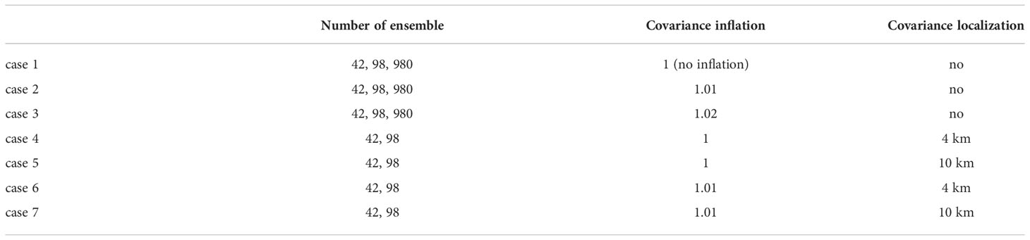
Table 3 Test cases of data assimilation.

The ensemble members were generated by adding noises to the amplitudes and phases of the five tidal constituents for both the tidal elevation and normal velocity at all open boundaries, following previous studies (Park and Kaneko, 2000; Lin et al., 2005; Zhu et al., 2017). The noises to the tidal elevation’s five constituents were generated from the normal distributions with zero mean and standard deviation of 10% (15% or 20%) of M2 (S2 or K1, O1, and N2) constituent’s amplitude and 2°, respectively. The corresponding amplitude of tidal elevation were 10.7, 7.1, 6.8, 4.4, and 4.4 cm for M2, N2, K1, O1, and N2 tidal constituents, respectively. We assumed that the normal velocities at open boundaries were more uncertain than the tidal elevation at the open boundaries. Thus, relatively large noises were added to the normal velocities at the open boundaries to generate ensemble members. The noises to the five tidal constituents of the normal velocity were generated from the normal distributions with zero mean and standard deviation of 10% (15% or 20%) of M2 (S2 or K1, O1, and N2) constituent’s amplitude and 20° for semi-diurnal tides and 10° for diurnal tides, respectively. The corresponding amplitudes of the normal velocity were 12.6, 7.4, 4.2, 1.8, and 5.2 cm s^-1 for M2, N2, K1, O1, and N2 tidal constituents, respectively. We also added noises to Manning’s roughness coefficient (n) and the lateral kinematic eddy viscosity coefficient (A_H). The noises to n and A_H were generated from the normal distributions with zero mean and standard deviation of 0.0002 and 0.4 m s^-2, respectively.

The velocity fields obtained from the data assimilation with the test cases in Table 3 were compared with the velocities obtained from the ADCP observations performed on October 30 and 31. Thus, we focused on assimilation results on October 30 and 31 in this paper. The model integration started at 00:00 on October 25, 2020, with no motion as the initial condition. The data assimilation step started at 16:00 on October 28, and the model state update was repeated every two minutes until 0:00 on November 1. The numerical model’s time integration in the first time step after updating state vector was replaced with the Euler method.

The comparison with the ADCP results was evaluated by correlation coefficient, root-mean-squared difference (RMSD), and fraction error variance (FEV). The definitions of the RMSD and fractional error variance are

$\begin{array}{ll}{\text{RMSD}}_U=\sqrt{\frac{1}{K}{\displaystyle \sum _i^K{(U_i^{\text{DA}}-U_i^{\text{ADCP}})}^2,}}& (16)\end{array}$

$\begin{array}{ll}{\text{RMSD}}_V=\sqrt{\frac{1}{K}{\displaystyle \sum _i^K{(V_i^{\text{DA}}-V_i^{\text{ADCP}})}^2}},& (17)\end{array}$

$\begin{array}{ll}\text{FEV}=\frac{{\displaystyle \sum {}_i^K}|(U_i^{DA}-U_i^{ADCP})+j(V_i^{DA}-V_i^{ADCP}){|}^2}{{\displaystyle \sum {}_i^K}|U_i^{ADCP}+j{V}_i^{ADCP}{|}^2},& (18)\end{array}$

where j×j=−1, K is the number of ADCP observation data, and |·| indicates computing the absolute value. For these comparisons, the data assimilation results were spatiotemporaly interpolated to obtain the velocity at the same locations and times as each ADCP velocity.

3 Results

The EnKF updates were performed with the cases listed in Table 3, and the resulting time series of velocity field was compared with the ADCP observed velocity. The results of the model prediction without the data assimilation was also compared with the ADCP results. Table 4 summarizes the results of the comparisons. The correlation coefficients of eastward and northward velocity between the model prediction and the ADCP results are 0.95 and 0.68, respectively. The RMSDs (RMSD_U and RMSD_V) are 0.29 and 0.20 m s^-1, and the fractional error variance is 19.6%. Although we implemented the information obtained from the observed path-averaged current into the open boundary condition in the numerical ocean model, there still were considerable differences from the ADCP results; thus, data assimilation is necessary.

TABLE 4

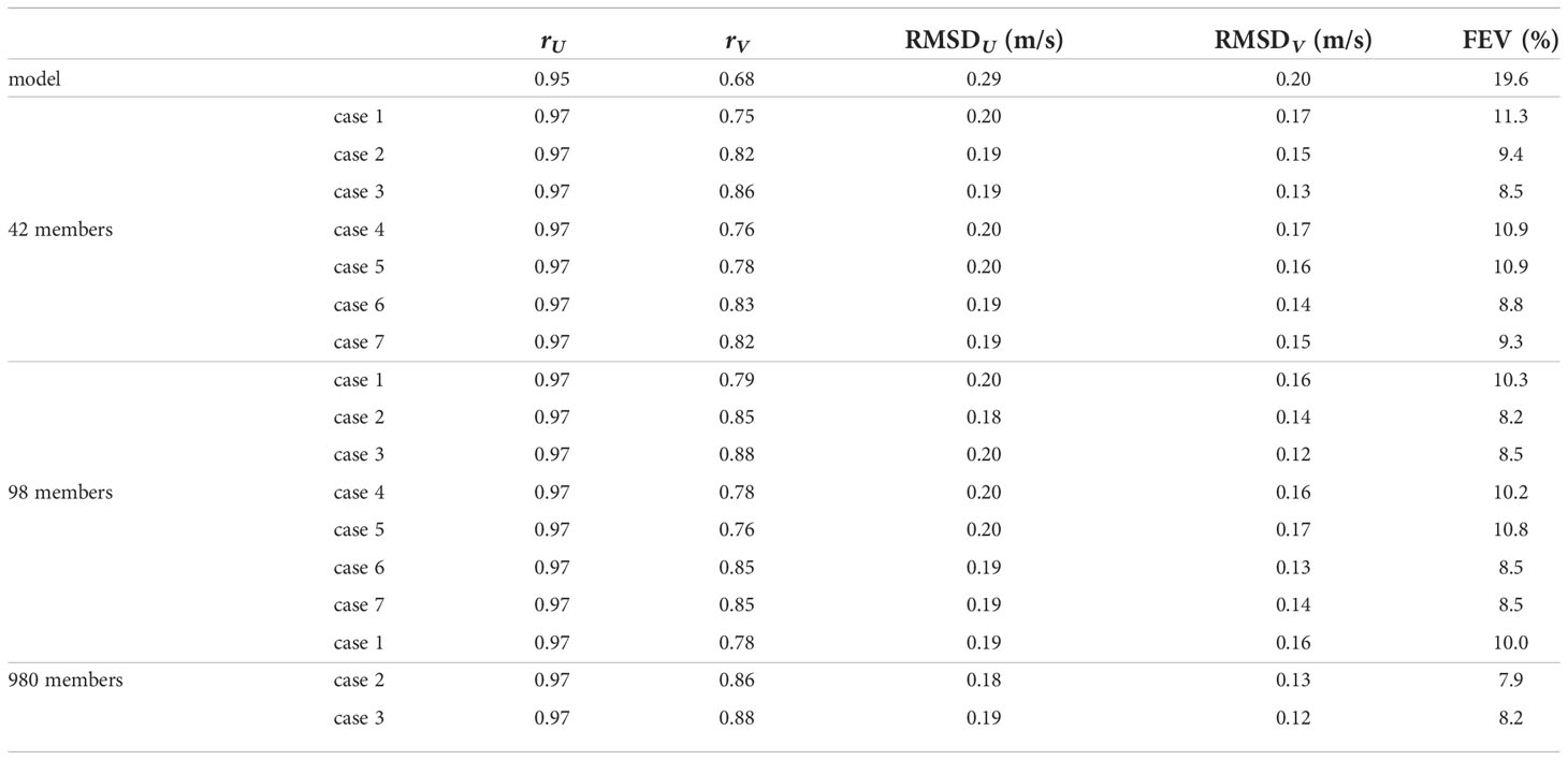
Table 4 Summary of the comparison with ADCP observed currents for all the test cases listed in Table 3.

The correlation coefficients of current velocity between the data assimilation and ADCP results are high. In particular, the correlation coefficients of the eastward current (r_U) are all 0.97. The correlation coefficients of the northward current is slightly lower than that of the eastward current but are still over 0.75. The RMSD is below 0.2 m s^-1 and the FEVs are about 8–11%. Implementing the covariance inflation improve the results compared with the results without the covariance inflation for all the tested ensemble member (test cases 2 and 3). On the other hand, implementing the covariance localization did not always reduce the RMSD or FEV. Implementing both covariance inflation and localization improved but was not always better than the results with covariance inflation only. There seems no clear difference between the results with covariance localization with different localization radii (cases 4 and 5, or 6 and 7). The test cases 2 and 3 with 980 ensemble members resulted in the smallest difference with reference to the ADCP results, but some cases with smaller ensemble member resulted in the similarly small differences (case 3 with 42 members and case 2 and 3 with 98 members).

Figure 4 shows the results with 980 ensemble members: the path-averaged currents predicted from the data assimilation results (left column) and the standard deviation of the path-averaged current ensembles (i.e., forecast ensemble spread; right column) for the five transmission paths. In general, the data assimilation results reproduced the observed path-averaged current patterns (black). However, the levels of fit are different between the test cases. Implementing the covariance inflation (red and yellow) and using the larger values (yellow) reproduced the path-averaged currents closer to the observed values. The case 2 with ρ_i=1.01 resulted in smaller FEV (7.9%) than that of case 3 (8.2%); however, in terms of the reproduced path-averaged currents, using ρ_i=1.02 may be desirable if one is interested in reproducing such high-frequency variation. The results without the covariance inflation (blue) could not reproduce some of the high-frequency variation, which might be under a filter divergence condition. The ensemble spread in the results with ρ_i=1 is nearly equal or somewhat larger than the assumed observation noise covariance (diagonal matrix with 0.025² m² s^-2). This indicates that even using large number of ensemble members can results in filter divergence if updating the state vector so often (2 min in this study); that is, the covariance inflation is necessary. The ensemble spread effectively enlarged by using the covariance inflation, in particular for the paths S1S2 and S3S4 (panel B1 and B5). For the path between S2 and S3, the path-averaged current observation failed during low tides because of the shallow bank near station S3 (Taniguchi et al., 2021b). During no observation, using ρ_i=1.02 caused relatively large ensemble spread (panel B3).

FIGURE 4

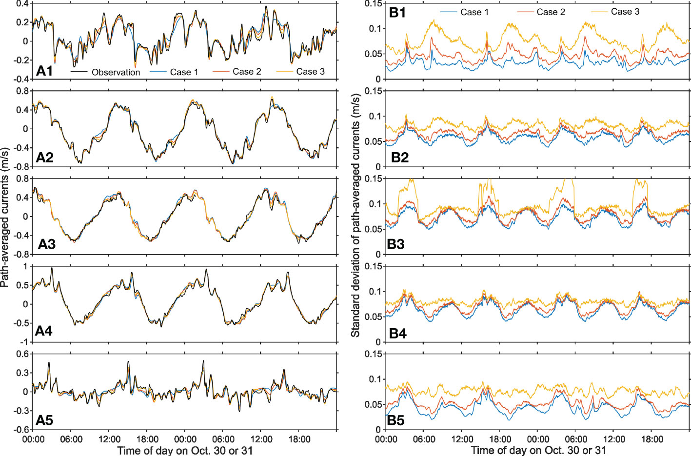
Figure 4 Results of data assimilation with 980 ensemble members. (A17–A5) Path-averaged currents along the station pairs S1S2, S1S3, S2S3, S2S4, and S3S4; (B1–B5) The standard deviation of path-averaged current ensembles (i.e., the forecast ensemble spread) just before the Kalman filter update in each transmission time for the same station pairs as of (A1–A5). The blue, red, and yellow lines are the results of cases 1, 2, and 3, respectively, and the black line in (A1–A5) indicates the observed path-averaged current.

Figures 5, 6 shows the same as Figure 4 but for the selected results (cases 1, 3, and 4) obtained from the data assimilation with 42 and 98 ensemble members. In the results with the 42 and 98 ensemble members, the path-averaged current reproduced from the data assimilation results agreed with the observed currents as is the case with the results of 980 ensemble members. The cases with covariance inflation (red) closely fit to the observed currents. The results with the covariance localization (yellow) did not improve the results much. It is also found that the difference between the data assimilation results and observed path-averaged current is smaller in the results with 980 ensemble members (gray in Figures 5A, 6A) than in 42 or 98 members.

FIGURE 5

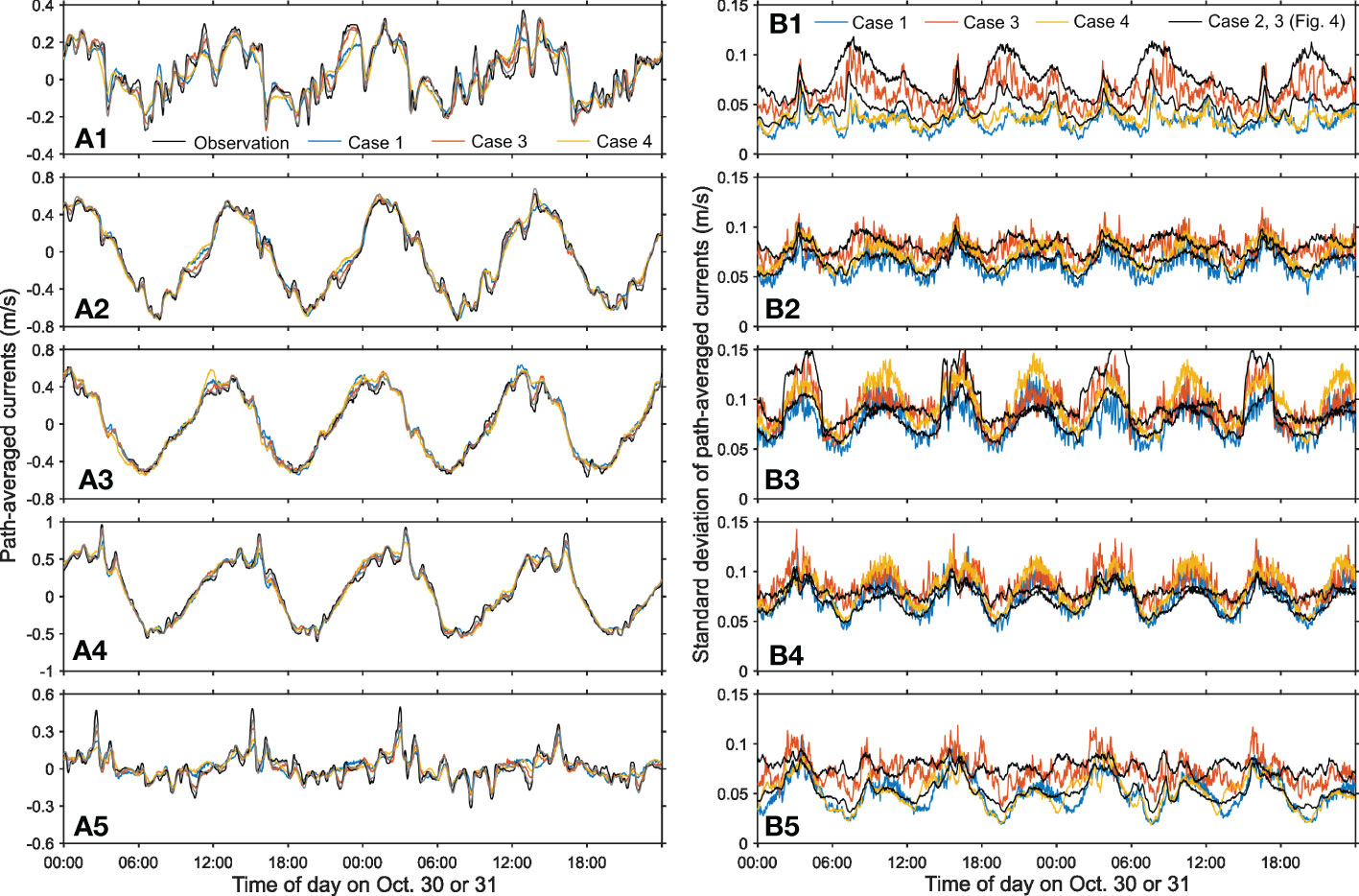
Figure 5 Same as Figure 3 but for the results of case 1 (blue), 3 (red), and 4 (yellow) with 42 ensemble members. The gray lines in panels (A1-A5) are the results of case 3 with 980 ensemble members. In panels (B1-B5), the two black lines are the results of case 2 and 3 with 980 ensemble members.

FIGURE 6

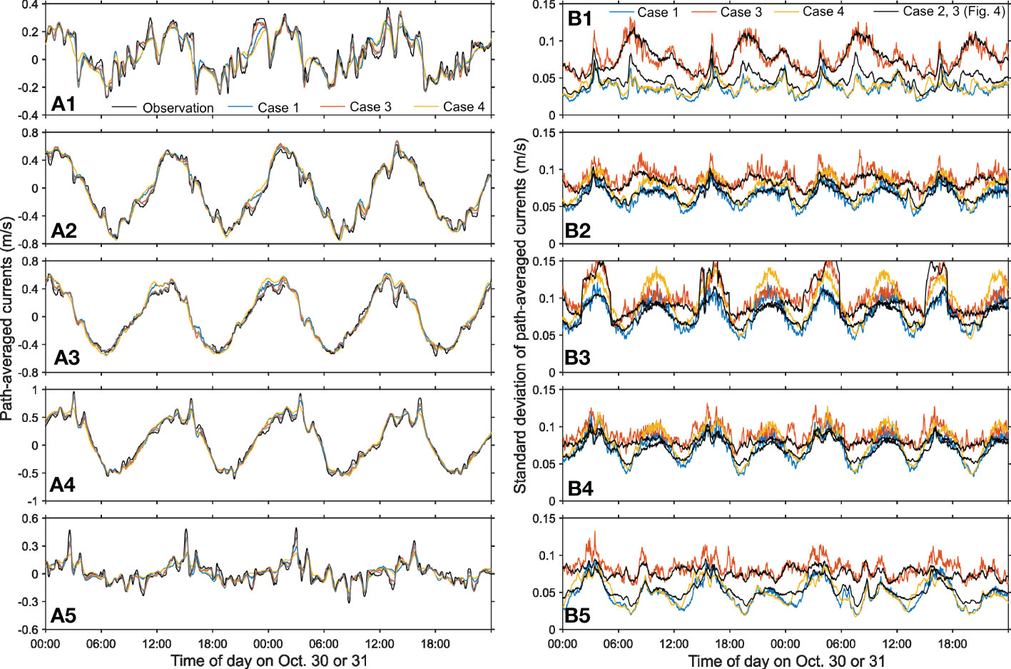
Figure 6 Same as Figure 4 but for the results of 98 ensemble members.

The ensemble spread in the results with 42 and 98 members shows that covariance inflation is also effective to enlarge the ensemble spread and to suppress filter divergence. The covariance localization does not always enlarge the ensemble spread; it is effective for the S2S3 and S2S4 paths (panels B3 and B4 in Figures 5, 6). For these paths, the ensemble spread of the test case 4 becomes sufficiently large during some specific periods. On the other hand, for the S1S2 and S3S4 paths, the ensemble spread is nearly equal to that of the results without both covariance localization and inflation. In the results with 42 and 98 members, it founds that the ensemble spread more fluctuates compared with the results with 980 members and even with the same covariance inflation value. The resulting ensemble spreads vary differently between the 98 (or 42) and 980 members.

The ADCP observed velocities and data assimilation results (case 3 with 98 ensemble members) are compared in Figure 7. Although only the results from one test case are shown in the figure, the results of other cases such as cases 2 and 3 with 980 ensemble members reproduced the nearly equivalent patterns of velocity fields. In the figure, the model predicted velocities are also compared with those of ADCP. While the model predicted velocities seems to reproduce the velocity patterns, but the discrepancy from the ADCP results are clearly found. In particular, the model prediction overestimates the velocity magnitude during the period with strong current. On the other hand, the data assimilation can reproduce the ADCP observed velocity patterns even the sharp spatial variation (e.g., the transects at 08:00 and 09:00 in panel B1). However, the velocity magnitude of data assimilation still slightly larger than that from ADCP observation during strong currents; the model’s overestimation was not perfectly corrected in the data assimilation results. The discrepancies between the data assimilation and ADCP results are also found near the coastlines (e.g., near the S4 station in the transects at 08:00 and 09:00 in panel B2) or around the curved flow during the period with weak currents (e.g., the transect at 12:00 in panel B3). There will be several reasons for this discrepancies between the data assimilation results and ADCP results during the weak currents. First, such weak current appears near the coastline, and the performance of the model (and assimilation too) may be restricted near the coastline because of the limited spatial resolution of the model. Also, there is no observation of path-averaged current along the coasts. Second, signal-to-noise ratio between the magnitude of tidal currents and assigned measurement noise become small during weak currents. Finally, tomographic path-averaged data are good at regularizing the red spectrum or fields with low wave number (e.g., Cornuelle and Worcester, 1996) like a nearly uniform flow during the strong current in the observation site, while the fields might be complex with vortex-shaped structures during weak currents (at slack water).

FIGURE 7

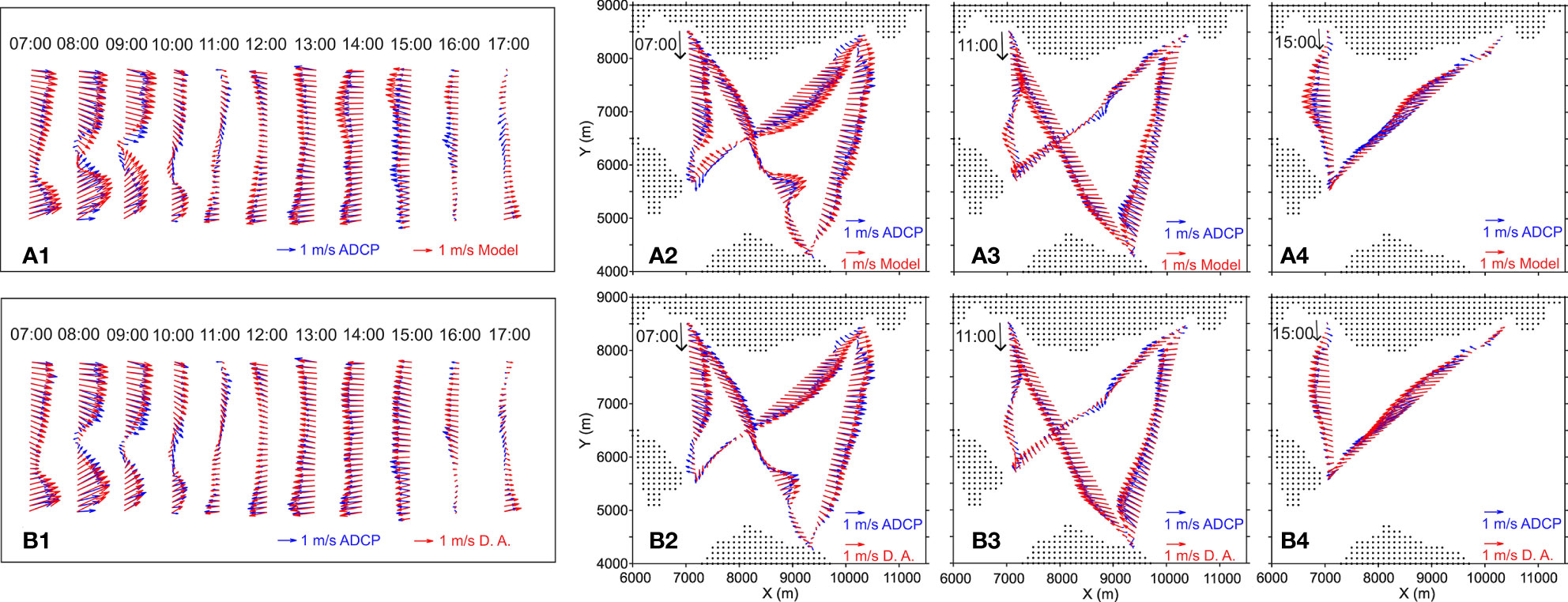
Figure 7 Comparison results of model prediction (panels A; first row) and data assimilation (panels B; second row) with the ADCP results. Panels (A1, B1) are the comparisons with the ADCP results on Oct. 30 (along the dashed line in Figure 1C), and panels (A2–A4, B2–B4) are the comparisons with the ADCP results on Oct. 31 (along the dotted lines in Figure 1C). The data assimilation result is obtained from case 3 with 98 ensembles.

In the results of our preliminary experiment along the S1 and S2 stations (Taniguchi et al., 2021a), the observed path-averaged current exhibited high-frequency oscillation with a period of about 1.5 h during the flood current. We can clarify the velocity fields causing those high-frequency variations with the data assimilation results. Figure 8 shows the time series of path-averaged currents along the S1 and S2 stations and six snapshots of the velocity fields during the periods with high frequency oscillation. The result used in the figure is from case 3 with 98 members. The observed and modeled results are also drawn in the path-averaged current’s time series plot. The data assimilation results reproduced the high-frequency variation in the observed path-averaged current (red and blue). The reproduced velocity snapshots exhibit the occurrence of a vortex at the island’s downstream (east) side. When the clockwise vortex exists behind the island, the path-averaged current exhibits a markedly sharp trend toward the S1 direction (at 7:30 and 9:00; panels C and F). On the other hand, when there is no clockwise vortex or an anticlockwise vortex behind the island, the path-averaged current has a trend in the direction of the S2 station (panels D, E, and G). That is, the high-frequency variation in the path-averaged current along the S1 and S2 stations during the flood tide is associated with the two vortex generations behind the island, i.e., due to the island wake. Note that the velocity fields at a northern part of the S1S2 path is nearly eastward and perpendicular to the path direction; thus, background eastward current less affect the variation in the S1S2 path-averaged current during the period. The numerical ocean model without data assimilation partly reproduced such island wake (the velocity fields are not shown here), but the occurrence timing and extent of the vortex were not well reproduced as we can expect from the model predicted path-averaged currents (the gray line in panel A).

FIGURE 8

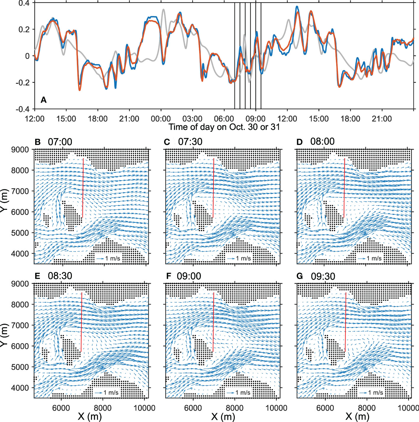
Figure 8 (A) Time series of path-averaged current between the S1 and S2 stations. The blue, red, and gray lines indicate the reciprocal acoustic transmission results, data assimilation results (case 3 with 98 members), and the model predictions, respectively. The positive value of the path-averaged currents corresponds to the flow toward the S1 station. Panels (B-G) show the snapshots of velocity fields at times shown as the vertical bars in (A). The red line in panels (B-G) is the path connecting the S1 and S2 stations.

In our previous report on this experiment, we showed that there were spike-like variations in the path-averaged currents between the S2 and S4 stations and the S3 and S4 stations with a slight time lag (Figure 4 in Taniguchi et al., 2021b). Such spike-like variation is found in almost every ebb tide. The velocity fields causing those spike-like variations are focused on in Figure 9. The model prediction did not reproduce the spike-like variation in the path-averaged current in the period shown in the figure but predicted several spike-like variation in other periods. The data assimilation result (case 3 with 98 ensemble members) reproduced the spike-like variation in the path-averaged currents (panels A1 and A2). Those spike-like variation may be associated with a strong current from the northeastern channel. During the period shown in Figures 9B, C, the relatively strong flow from the northeastern channel cross the S3S4 path with a slight angle; thus, the S3S4 path-averaged current shows rapid velocity variation toward negative value (toward the S3 station) at that time. During the same period, the flow is almost westward around the S2S4 path; thus, the path-averaged current between the S2 and S4 stations exhibits relatively large values. Then the area of the flow from the southeastern channel broadens northward (panels D and E). This variation cancels the contribution of the flow from the northeastern and southeastern channels to the path-averaged current along the S3S4 path, resulting in a path-averaged current with nearly zero. At the same time, strong flow from the northeastern channel reaches near the S2S4 path with the flow direction parallel to the path, causing further large (in the direction to S2 station) path-averaged current along the S2 and S4 stations. After that, the path-averaged current along both paths becomes nearly zero due to slack water (panel G). The path-averaged currents contain velocity information on both the magnitude and direction, and thus, the path-averaged current express rapid variation when both the magnitude and direction simultaneously cause the variation in the same sign (positively or negatively). The reproduced current velocity fields also exhibit markedly curved flow around the path between the S2 and S3 stations during the last half period (panels E and F); however, the period corresponds to low tide (Figure 3), and the transmission between the S2 and S3 station failed due to shallow bank near the S3 station. Thus, the velocity patterns near the S2S3 path can be somewhat uncertain. Applying data assimilation with successful five path-averaged currents will better clarify the velocity field time variation related to the spike-like variation in the path-averaged currents.

FIGURE 9

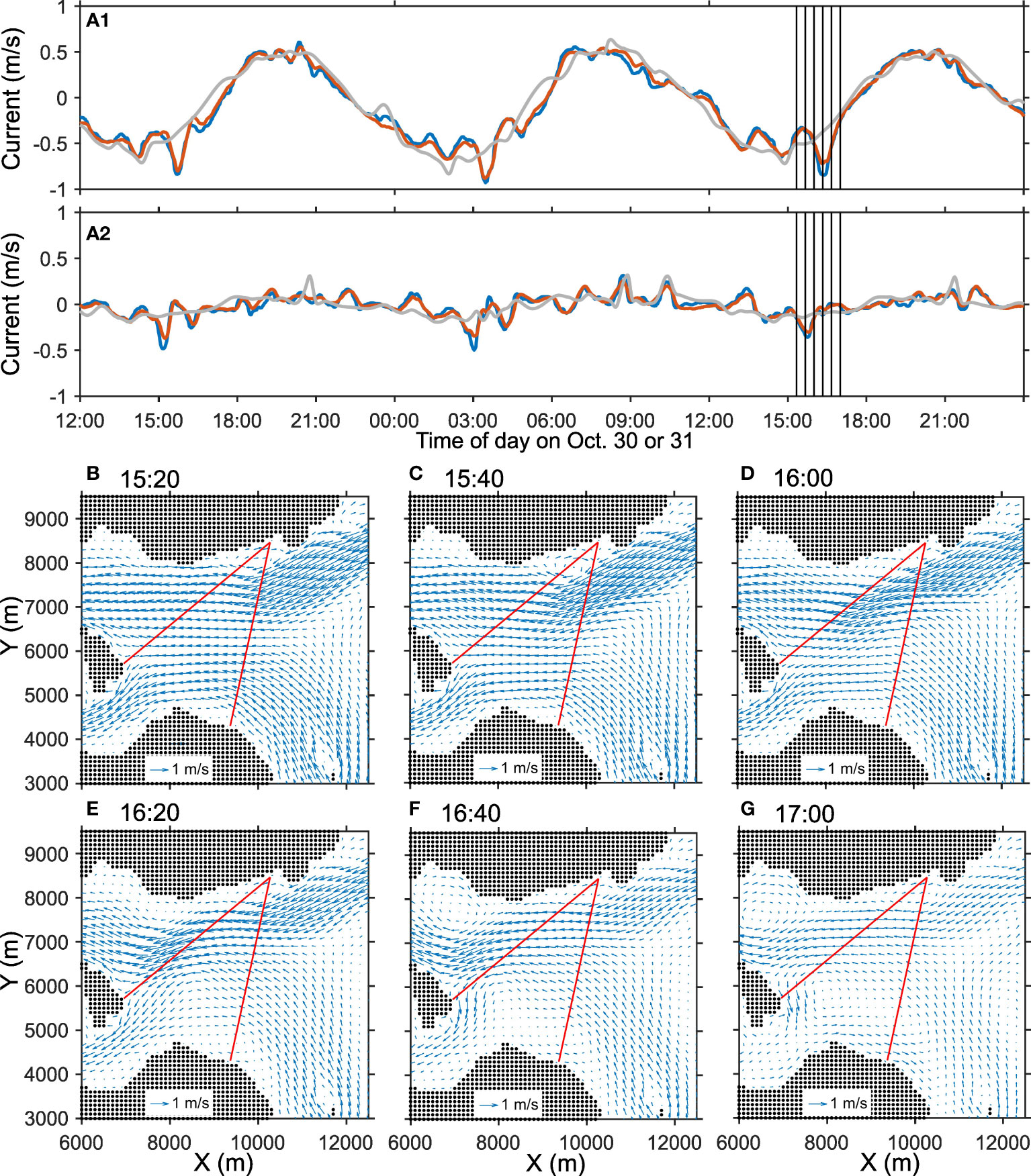
Figure 9 (A1, A2) time series of path-averaged current between the S2 and S4 stations and the S3 and S4 stations. The blue, red, and gray lines indicate the reciprocal acoustic transmission results, data assimilation results (case 3 with 98 members), and the model predictions, respectively. The positive value of the path-averaged currents corresponds to the flow toward the S4 station for both station pairs. Panels (B-G) show the snapshots of velocity fields at times shown as the vertical bars in (A). The red lines in panels (B-G) are the paths connecting the S2 and S4 stations and the S3 and S4 stations.

4 Discussion

The performance of EnKF with the several combination of covariance localization and inflation, and the number of ensemble member are investigated via the comparison with the ADCP results. These factors relate with the issues introduced by ensemble approximation of covariance matrix in Kalman filter: spurious correlation and filter divergence. These factors have not always been considered in the previous CAT studies (Park and Kaneko, 2000; Lin et al., 2005; Zhu et al., 2017). This may be because, in these studies (and in this study), the ensemble members are generated by adding noises to the open boundary forcing. Velocities around the open boundary are always different over ensemble members, and thus, permanent filter divergence do not occur, leading to somewhat untouched theme in the CAT data assimilation. However, as shown in this paper, covariance inflation, which spread ensembles after each updates, improves both the level of fit to the observed path-averaged currents and agreement with the ADCP result. In the present study, the constant inflation value of 1.01 or 1.02 worked and improved the results. With the covariance inflation, the difference of the results was minor between 98 and 980 ensemble members regarding the comparisons with the ADCP results. One note is that the numerical experiments shown in Table 4 were from the results of one realization for each test case. As the results (Figures 4–6) indicates, the results may depend on the noise added to the observed data (i.e., to make perturbed observation) and boundary condition, and the sensitivity to the added noise are larger with smaller ensemble members. Thus, the results in Table 4 may slightly change with different ensemble realizations; however, the superiority with covariance inflation and with larger ensemble members will be retained.

Low quality of assimilation results without covariance inflation is due to frequent update by observation with relatively small observational error (0.025 m s^-1). With frequent Kalman updates, ensembles may not spread sufficiently between updates and the next updates, leading to temporary filter divergence in some period. Thus, covariance inflation is required to inflate the analysis ensemble even with many ensembles. This indicates that the time interval between the Kalman updates may be extended although we conducted the acoustic transmission and the Kalman updates every two minutes. Note that however, there is flow patterns that cause spike-like or triangle-shape variation in the path-averaged currents (Taniguchi et al., 2021a; Taniguchi et al., 2021b); thus, one still needs high-frequent transmissions to measure (record) the path-averaged currents as references. Also, sufficiently frequent measurements and updates can recursively pull the ensembles toward the measured solution and do not allow the ensembles to diverge (to bimodal) even in strongly nonlinear dynamics (Evensen et al., 2022).

The comparisons with ADCP results suggest that covariance localization is not required if one focuses only inside the tomographic array. Here, we consider the performance differences in terms of spatial structure of covariance. Figure 10 shows the spatial map of ensemble correlation associated with cross-covariance ${\tilde{\mathit{E}}}_k{(\mathit{H}{\tilde{\mathit{E}}}_k)}^{\text{T}}$ in Eq. (13) (i.e., cross-covariance between the velocity field ensembles and path-averaged current ensembles) for eastward (U) and northward (V) components at a specific time of 9:00 on October 31, 2020. The results of the test case 3 with ensemble members of 980, 98, and 42, and the test case 4 with 42 ensemble members are shown. The results with 980 ensemble members (the first rows of panels A and B) shows high-correlation patches along the paths. In addition, there are weak correlations between each path-averaged current and velocity fields throughout the model domain. The results with 980 ensemble members had less spurious correlation because of sufficient number of ensemble members; thus, these weak spatial-correlations are physical correlations of tidal currents. Also, some of these spatial-correlation is partly explained by the characteristic of integral observations (path-averaged currents). As van Leeuwen (2019) demonstrated, non-local measurements (i.e., path-averaged currents) can influence distant state variables, which are not physically connected in the prior covariance but become connected via the non-local observation. The velocity fields throughout the model domain including those at open boundaries are corrected by the data assimilation via these correlation, and it is reasonable that the covariance localization is not required for this case. The results with 98 ensemble members (the second rows of panels A and B) show similar spatial structures of correlation but with slightly complex and higher (positively or negatively) correlation values, in particular, at outside the area covered by the reciprocal acoustic transmission. The results with 42 ensemble members (the third rows of panels A and B) show further spatially high-correlations. These correlations higher than that in the results of 980 ensemble members would be spurious correlation associated with insufficient ensemble members and sampling errors. However, if we focus on the area covered by reciprocal acoustic transmissions, the spatial patterns are retained even in the results with 42 ensemble members, resulting in similar performances between them (FEVs of 8.2, 8.5, and 8.5, respectively, when 980, 98, and 42 ensemble member were used). Short interval of Kalman update (2 minutes) is also responsible for the nearly equal performances.

FIGURE 10

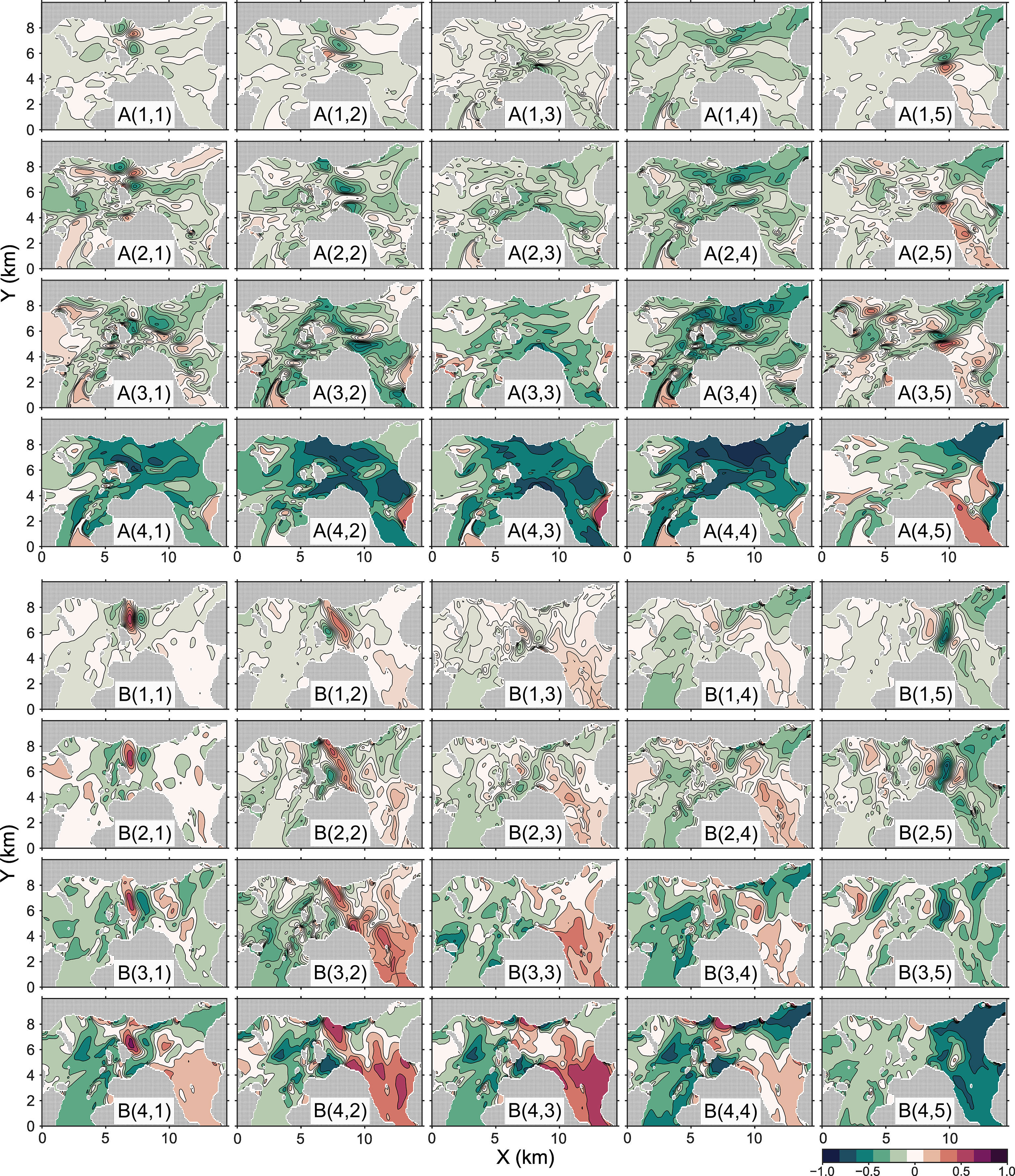
Figure 10 Spatial map of ensemble correlation associated with cross-covariance Ẽ_k(HẼ_k)^T in Eq. (13) for eastward (U; panels A) and northward (V; panels B) components at a specific time of 9:00 on October 31, 2020. In each panel (A, B), the first, second, and third rows show the results of case 3 with 980, 98, and 42 ensemble members, and the fourth row shows the result of case 4 with 42 ensemble members (see Table 3 for the test case). The column number indicates the station pair of the path-averaged currents: S1S2, S1S3, S2S3, S2S4, and S3S4, from the left to right column.

Figure 10 also shows the results of case 4 with 42 ensemble members (the fourth rows of panels A and B), which implemented the covariance localization with a localization radius of 4 km. The results with 42 ensemble members with covariance localization shows further high-correlation. This is because Kalman updates are limited to the center of the observation area and the model ensemble predictions are somewhat retained even along the reciprocal acoustic transmission paths. It is also noted that the small spatial structures of correlation found in the results without covariance localization (from the first to third rows) are weaken in the results with 42 ensemble members with covariance localization. It is naturally expected that EnKF does not properly updates the velocity fields with the structures found in the results without the covariance localization. In fact, Cornuelle and Worcester (1996) used simple numerical experiments and showed that the data assimilation with integral observations requires retaining full information in a model covariance matrix, i.e., off-diagonal components in model covariance matrix is important. Since the covariance localization, with a short localization radius in particular, quickly decreases the off-diagonal terms (as well as diagonal terms far from the observation location) to zeros, it makes Kalman filter not optimal scheme for integral data such as path-averaged currents. However, if we need to run the EnKF with further smaller number of ensemble members such as 20 (Zhu et al., 2017), spurious correlation will be more significant and affect the assimilation results. For such case, the covariance localization can be used to mitigate spurious correlation. When we performed the same numerical experiments with 20 ensemble members, the fractional error variance (FEV) were 15.6%, 10.2%, 10.0%, 11.6%, 12.0%, 9.9%, and 11.2% for the Case 1 to Case 7, respectively.

The velocity fields reproduced by the data assimilation revealed the reasons for the high-frequency or spike-like variations in the observed path-averaged currents (Taniguchi et al., 2021a; Taniguchi et al., 2021b). The high-frequency variation in the path-averaged current along the S1 and S2 stations is associated with the island wake. The data assimilation results revealed the repeated occurrences of clockwise and anticlockwise vortexes behind the island. It is noted that the numerical model potentially included the responsible mechanisms to reproduce the island wakes (the gray line in Figure 7). However, it would be unable to reproduce the island wake precisely by the numerical model alone with limited open boundary condition (only five tidal constituents with constant velocity along the boundary and no tangential velocity), because the extents and timings of wake generations are complex and vary with every flood tides, as expected by the time series plots of the S1S2 path-averaged current (Figure 8 and Figure 8 in Taniguchi et al., 2021a). The island wake is a research topic in the geophysical fluid dynamics over a long period, and even today, there have been studies associated with the island wake (e.g., Chang et al., 2013; Chang et al., 2019). The period of wake evolution T is related to the Strouhal number S_t=D/UT where D and U are the characteristic length of the island and the reference velocity. With approximate values of D=1.5 km (the north-south length), U=1.5 m s^-1, and T=1.5 h, we obtain S_t=0.185, which is close to the rough value of S_t (about 0.2) with a range of Reynolds number 200–2×10⁵. If we measure the vortex shedding period T and estimate the flow velocity, it would be regarded as a real-field application of the vortex flowmeter. The high-frequency variation in the S1S2 path-averaged current is not clear in the path-averaged current along the S3S4 path, which contain the northward velocity component same as the S1S2 path; thus, at this moment, it is expected that the vortexes quickly decay or corrupt. The data assimilation results also do not contain clear vortex street. Additional observation to sample the vortex in various angles will be required to reproduce the vortex generation, shape, downstream movement, and/or corruption more precisely. The island wake occurs almost every flood tide but only during a short period. For such a short observation period, a moving ship acoustic tomography (Huang et al., 2019) may be effectively used to improve the reproduction performance.

5 Summary and concluding remarks

In this paper, we investigated the performance of CAT data assimilation by applying EnKF to the path-averaged currents obtained from the 2020 reciprocal acoustic transmission experiment with four acoustic stations deployed at Mihara-Seto in the Seto Inland Sea, Japan. The results of EnKF with several combinations of the values of covariance localization, inflation, and the number of ensemble members were compared with the ADCP results. The results showed that data assimilation with EnKF improved the velocity reproduction compared with the model prediction and that implementing covariance inflation contributed to additional improvements for all the tested ensemble members. Thus, it is suggested that the covariance inflation should be implemented in CAT data assimilation with EnKF, in particular, when EnKF updates are performed frequently. Focusing on the velocity fields inside the tomographic array, we obtained nearly equivalent performance of EnKF over 98 and 980 ensemble members with covariance inflation. The covariance localization did not improve the results for the number of ensemble members of 42, 98 and 980.

In this study, we implemented EnKF as the data assimilation scheme for path-averaged currents, but this does not mean that EnKF always provides the best estimates. Rather, in our study, we purpose developing a near-real-time (nowcasting) tidal current reproducing system, and EnKF is suitable to implement as the term filter indicates (i.e., not the smoother). If the purpose is hindcasting, then ensemble Kalman smoother may provide better estimates (Evensen, 2009). Also, we did not explore the applicability of other data assimilation schemes such as square-root-filter, which would provide better performance when the ensemble member is small.

With the above-mentioned limitation, the obtained comparison results provide some guides when CAT data assimilation with EnKF is applied. The reproduced velocity fields agreed with the ADCP results; the fractional error variance is about 8%. Additional improvements would be possible by successful transmissions over all the five paths. The data assimilation results also revealed the reason for the high-frequency variation in the path-averaged currents found in the previous reciprocal acoustic transmission experiment conducted in the same area (Taniguchi et al., 2021a). The repeated generation (but only two or three) of vortexes during the flood tide at the downstream side of the island (i.e., island wakes) caused high-frequency variation in the path-averaged current. This, in turn, indicates that the reciprocal acoustic transmission and the resulting path-averaged current can be used to effectively detect temporal variation in the velocity fields associated with island wakes. Thus, while previous CAT studies have showed its usefulness, this study is an additional example demonstrating the usefulness of CAT as an observational method for the studies on coastal physical processes.

Data availability statement

The raw data supporting the conclusions of this article will be made available by the authors, without undue reservation.

Author contributions

NT, HM, and TT contributed to conception and design of the study. NT, TT, KY, HY, YS, and KH provided instrument resources and/or performed field observation, contributed to data acquisition. NT, MA, and HM contributed model development and validation. NT, TT, and KH contributed to data analysis methodology. NT wrote the first draft of the manuscript. HM, MA, YS, and TT wrote sections of the manuscript. All authors contributed to the article and approved the submitted version.

Funding

This work was partly supported by JSPS KAKENHI Grant Numbers 19H04292, 20H02369, 20K14964, 22K04563.

Acknowledgments

The authors are grateful to Geinan Fisheries Cooperative Association, Mihara-Shi Fisheries Cooperative Association, Ohmishima (Ehime Prefecture) Fisheries Cooperative Association, and TSUNEISHI SHIPBUILDING Co., Ltd. for their support in the reciprocal acoustic transmission experiment. The Sentinel-2 image in Figure 1 was downloaded from the EO browser (https://www.sentinel-hub.com/explore/eobrowser/).

Conflict of interest

Author TT, KY, and HY are employed by Fukken Co., LTD.

The remaining authors declare that the research was conducted in the absence of any commercial or financial relationships that could be construed as a potential conflict of interest.

Publisher’s note

All claims expressed in this article are solely those of the authors and do not necessarily represent those of their affiliated organizations, or those of the publisher, the editors and the reviewers. Any product that may be evaluated in this article, or claim that may be made by its manufacturer, is not guaranteed or endorsed by the publisher.

References

Anderson J. L., Anderson S. L. (1999). A monte carlo implementation of the nonlinear filtering problem to produce ensemble assimilations and forecasts. Monthly Weather Rev. 127, 2741–2758. doi: 10.1175/1520-0493(1999)127<2741:AMCIOT>2.0.CO;2

CrossRef Full Text | Google Scholar

Blumberg A. F., Mellor G. L. (1987). A description of a three-dimensional coastal ocean circulation model. In Three-Dimensional Coastal Ocean Models. Heaps N. S. Ed. doi: 10.1029/CO004p0001

CrossRef Full Text | Google Scholar

Burgers G., van Leeuwen P. J., Evensen G. (1998). Analysis scheme in the ensemble kalman filter. Monthly Weather Rev. 126, 1719–1724. doi: 10.1175/1520-0493(1998)126<1719:ASITEK>2.0.CO;2

CrossRef Full Text | Google Scholar

Carter G. S., Merrifield M. A. (2007). Open boundary conditions for regional tidal simulations. Ocean Model. 18, 194–209. doi: 10.1016/j.ocemod.2007.04.003

CrossRef Full Text | Google Scholar

Chang M.-H., Jan S., Liu C.-L., Cheng Y.-H., Mensah V. (2019). Observations of island wakes at high rossby numbers: Evolution of submesoscale vortices and free shear layers. J. Phys. Oceanogr. 49, 2997–3016. doi: 10.1175/JPO-D-19-0035.1

CrossRef Full Text | Google Scholar

Chang M.-H., Tang T. Y., Ho C.-R., Chao S.-Y. (2013). Kuroshio-induced wake in the lee of green island off taiwan. J. Geophys. Res.: Oceans 118, 1508–1519. doi: 10.1002/jgrc.20151

CrossRef Full Text | Google Scholar

Chen H., Chen H., Zhang Y., Xu W. (2021). Decentralized estimation of ocean current field using underwater acoustic sensor networks. J. Acoustical Soc. America 149, 3106–3121. doi: 10.1121/10.0004795

CrossRef Full Text | Google Scholar

Chen M., Kaneko A., Lin J., Zhang C. (2017). Mapping of a typhoon-driven coastal upwelling by assimilating coastal acoustic tomography data. J. Geophys. Res.: Oceans 122, 7822–7837. doi: 10.1002/2017JC012812

CrossRef Full Text | Google Scholar

Chen Y., Oliver D. S. (2017). Localization and regularization for iterative ensemble smoothers. Comput. Geosci. 21, 13–30. doi: 10.1007/s10596-016-9599-7

CrossRef Full Text | Google Scholar

Cornuelle B. D., Worcester P. F. (1996). “Ocean acoustic tomography: Integral data and ocean models,” in Modern approaches to data assimilation in ocean modeling, vol. 61 . Ed. Malanotte-Rizzoli P. (Amsterdam: Elsevier Oceanography Series), 97–115. doi: 10.1016/S0422-9894(96)80007-9

CrossRef Full Text | Google Scholar

Cornuelle B., Munk W., Worcester P. (1989). Ocean acoustic tomography from ships. J. Geophys. Res. 94 (C5), 6232–6250. doi: 10.1029/JC094iC05p06232

CrossRef Full Text | Google Scholar

Evensen G. (1994). Sequential data assimilation with a nonlinear quasi-geostrophic model using Monte Carlo methods to forecast error statistics. J. Geophys. Res.: Oceans 99, 10143–10162. doi: 10.1029/94JC00572

CrossRef Full Text | Google Scholar

Evensen G. (2003). The ensemble kalman filter: Theoretical formulation and practical implementation. Ocean Dynamics 53, 343–367. doi: 10.1007/s10236-003-0036-9

CrossRef Full Text | Google Scholar

Evensen G. (2009). Data assimilation: The ensemble kalman filter. earth and environmental science (Berlin Heidelberg: Springer).

Google Scholar

Evensen G., Vossepoel F., Leeuwen P. J. (2022). Data Assimilation Fundamentals. Cham: Springer International Publishing. p. 245. doi: 10.1007/978-3-030-96709-3

CrossRef Full Text | Google Scholar

Gaspari G., Cohn S. E. (1999). Construction of correlation functions in two and three dimensions. Q. J. R. Meteorol. Soc. 125, 723–757. doi: 10.1002/qj.49712555417

CrossRef Full Text | Google Scholar

Hamill T. M., Whitaker J. S., Snyder C. (2001). Distance-dependent filtering of background error covariance estimates in an ensemble kalman filter. Monthly Weather Rev. 129, 2776–2790. doi: 10.1175/1520-0493(2001)129<2776:DDFOBE>2.0.CO;2

CrossRef Full Text | Google Scholar

Howe B. M., Worcester P. F., Spindel R. C. (1987). Ocean acoustic tomography: Mesoscale velocity. J. Geophys. Res.: Oceans 92, 3785–3805. doi: 10.1029/JC092iC04p03785

CrossRef Full Text | Google Scholar

Huang C.-F., Li Y.-W., Taniguchi N. (2019). Mapping of ocean currents in shallow water using moving ship acoustic tomography. J. Acoustical Soc. America 145, 858–868. doi: 10.1121/1.5090496

CrossRef Full Text | Google Scholar

Huang C.-F., Yang T. C., Liu J.-Y., Schindall J. (2013). Acoustic mapping of ocean currents using networked distributed sensors. J. Acoustical Soc. America 134, 2090–2105. doi: 10.1121/1.4817835

CrossRef Full Text | Google Scholar

Kaneko A., Zhu X.-H., Lin J. (2020). Coastal acoustic tomography (Amsterdam: Elsevier). doi: 10.1016/C2018-0-04180-8

CrossRef Full Text | Google Scholar

Kawanisi K., Zhu X.-H., Fan X., Nistor I. (2017). Monitoring tidal bores using acoustic tomography system. J. Coast. Res. 33, 96–104. doi: 10.2112/JCOASTRES-D-15-00172.1

CrossRef Full Text | Google Scholar

Lin J., Kaneko A., Gohda N., Yamaguchi K. (2005). Accurate imaging and prediction of kanmon strait tidal current structures by the coastal acoustic tomography data. Geophys. Res. Lett. 32, L14607. doi: 10.1029/2005GL022914

CrossRef Full Text | Google Scholar

Munk W., Worcester P., Wunsch C. (1995). Ocean acoustic tomography. Cambridge monographs on mechanics (Cambridge: Cambridge University Press). doi: 10.1017/CBO9780511666926

CrossRef Full Text | Google Scholar

Munk W., Wunsch C. (1979). Ocean acoustic tomography: a scheme for large scale monitoring. Deep Sea Res. Part A. Oceanogr. Res. Papers 26, 123–161. doi: 10.1016/0198-0149(79)90073-6

CrossRef Full Text | Google Scholar

Ogasawara H., Mori K. (2016). Acoustical environment measurement at a very shallow port: Trial case in hashirimizu port. Japanese J. Appl. Phys. 55, 07KE17. doi: 10.7567/jjap.55.07ke17

CrossRef Full Text | Google Scholar

Park J.-H., Kaneko A. (2000). Assimilation of coastal acoustic tomography data into a barotropic ocean model. Geophys. Res. Lett. 27, 3373–3376. doi: 10.1029/2000GL011600

CrossRef Full Text | Google Scholar

Taniguchi N., Takahashi T., Yoshiki K., Yamamoto H., Hanifa A. D., Sakuno Y., et al. (2021a). A reciprocal acoustic transmission experiment for precise observations of tidal currents in a shallow sea. Ocean Eng. 219, 108292. doi: 10.1016/j.oceaneng.2020.108292

CrossRef Full Text | Google Scholar

Taniguchi N., Takahashi T., Yoshiki K., Yamamoto H., Sugano T., Mutsuda H., et al. (2021b). Reciprocal acoustic transmission experiment at mihara-seto in the seto inland Sea, Japan. Acoustical Sci. Technol. 42, 290–293. doi: 10.1250/ast.42.290

CrossRef Full Text | Google Scholar

Trump C. L., Marmorino G. O. (1997). Calibrating a gyrocompass using ADCP and DGPS data. J. Atmospheric Oceanic Technol. 14, 211–214. doi: 10.1175/1520-0426(1997)014<0211:CAGUAA>2.0.CO;2

CrossRef Full Text | Google Scholar

van Leeuwen P. J. (2019). Non-local observations and information transfer in data assimilation. Front. Appl. Mathematics Stat 5. doi: 10.3389/fams.2019.00048

CrossRef Full Text | Google Scholar

Wang T., Zhang Y., Yang T. C., Chen H., Xu W. (2018). Physics-based coastal current tomographic tracking using a kalman filter. J. Acoustical Soc. Am. 143, 2938–2953. doi: 10.1121/1.5036755

CrossRef Full Text | Google Scholar

Williams P. D. (2009). A proposed modification to the Robert—Asselin time filter. Monthly Weather Rev. 137, 2538–2546. doi: 10.1175/2009MWR2724.1

CrossRef Full Text | Google Scholar

Worcester P. F. (1977). Reciprocal acoustic transmission in a midocean environment. J. Acoust. Soc Am. 62, 895–905. doi: 10.1121/1.381619

CrossRef Full Text | Google Scholar

Zheng H., Gohda N., Noguchi H., Ito T., Yamaoka H., Tamura T., et al. (1997). Reciprocal sound transmission experiment for current measurement in the seto inland Sea, Japan. J. Oceanogr. 53, 117–127.

Google Scholar

Zhu Z.-N., Zhu X.-H., Guo X., Fan X., Zhang C. (2017). Assimilation of coastal acoustic tomography data using an unstructured triangular grid ocean model for water with complex coastlines and islands. J. Geophys. Res.: Oceans 122, 7013–7030. doi: 10.1002/2017JC012715

CrossRef Full Text | Google Scholar

Zhu Z.-N., Zhu X.-H., Zhang C., Chen M., Wang M., Dong M., et al (2021). Dynamics of tidal and residual currents based on coastal acoustic tomography assimilated data obtained in Jiaozhou Bay, China. J. Geophys. Res.: Oceans 126, e2020JC017003. doi: 10.1029/2020JC017003

CrossRef Full Text | Google Scholar

Zhu Z.-N., Zhu X.-H., Guan W., Zhang C., Chen M., Liu Z.-J., et al (2022). Synchronous Assimilation of Tidal Current-Related Data Obtained Using Coastal Acoustic Tomography and High-Frequency Radar in the Xiangshan Bay, China. Remote Sens. 14, 3235. doi: 10.3390/rs14133235

CrossRef Full Text | Google Scholar