A hybrid deep learning model for predicting the Kuroshio path south of Japan

At present, many prediction models based on deep learning methods have been widely used in ocean prediction with satisfactory results. However, few deep learning models are used to predict the Kuroshio path south of Japan. In this study, a hybrid deep learning prediction model is constructed based on the long short-term memory (LSTM) neural network, combined with the complex empirical orthogonal function (CEOF) and bivariate empirical mode decomposition (BEMD), called CEOF-BEMD-LSTM. We train the model by using a 50-year (1958-2007) long time series of daily mean positions of the Kuroshio path south of Japan extracted from a regional ocean reanalysis dataset. During the test period of 15 years (2008-2022) by using daily altimetry dataset, our model shows a good performance for the Kuroshio path prediction with the lead time of 120 days, with 0.44° root-mean-square error (RMSE) and 0.75 anomaly correlation coefficient (ACC). This model also has good prediction skill score (SS). Moreover, the CEOF-BEMD-LSTM model successfully hindcasts the formation of the latest Kuroshio large meander since the summer of 2017. Predictions of the Kuroshio path for the coming 120 days (from January1 to April 30, 2023) indicate that the Kuroshio will continue to remain in the state of the large meander. Besides, predictor(s) of the Kuroshio path south of Japan need to be sought and added in future research.

1 Introduction

The Kuroshio is the western boundary current of the North Pacific Subtropical Gyre. It originates from the bifurcated North Equatorial Current on the eastern side of the Philippines, flows into the East China Sea via the east of Taiwan Island, and then veers eastward through the Tokara Strait into the sea south of Japan (Usui et al., 2006; Usui, 2019; Qiu et al., 2021). As the second warmest current globally, the Kuroshio brings a large amount of heat to the southern coast of Japan (Tsujino et al., 2006). Due to topographic constraints, the Kuroshio path south of Japan exhibits three typical paths (Kawabe, 1995): the typical large meander (tLM) path, offshore non-large meander (oNLM) path, and nearshore non-large meander (nNLM) path (Figure 1). The variation of the Kuroshio path has large effects on climate, fisheries, and ship navigation (Nakata et al., 2000; Tsujino et al., 2006; Sugimoto et al., 2020; Sugimoto et al., 2021). Therefore, it is of great significance to conduct prediction of the Kuroshio path south of Japan.

FIGURE 1

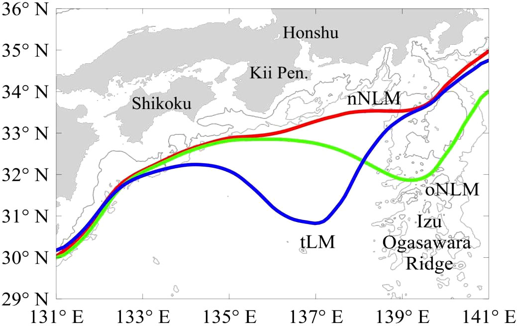
Figure 1 Three typical Kuroshio paths south of Japan: nNLM (red line), oNLM (green line), and tLM (blue line) derived from a regional ocean reanalysis described in section 2.1. Thin black contours are isobaths of 1 000 and 2 000 m.

Numerical prediction plays a dominant role in predicting the variation of the Kuroshio path south of Japan. Several studies used experiments to predict the variability of the Kuroshio path using data assimilation models, and the results showed that the predictive limit for the Kuroshio path south of Japan is about a couple of months (Komori et al., 2003; Kamachi et al., 2004; Miyazawa et al., 2005; Usui et al., 2006). The Japan Coastal Ocean Predictability Experiment (JCOPE), which is aimed to describe the Kuroshio path, Kuroshio Extensions, and Oyashio variability (Miyazawa et al., 2008; Miyazawa et al., 2009); It provides the Kuroshio prediction two months ahead of time.

As one of the most popular and consequential technologies, deep learning methods have been widely used for ocean prediction (Reichstein et al., 2019). Among them, the recurrent neural network (RNN) and its variants are known to work well in processing time series data to find the time-varying principles hidden in the time series data (Song et al., 2020). The long short-term memory (LSTM) neural network, as one of the essential variants of the RNN, can detect even minor changes from the time series and avoids the problem of vanishing gradient and exploding gradient (Hochreiter and Schmidhuber, 1997). In recent years, the LSTM neural network had a good performance in the time series prediction of ocean variables (Liu et al., 2018; Xiao et al., 2019; Shao et al., 2021b). However, few deep learning models are used to predict the Kuroshio path south of Japan.

In this study, we present a hybrid deep learning prediction model, combining the complex empirical orthogonal function (CEOF) analysis, bivariate empirical mode decomposition (BEMD) analysis, and LSTM neural network, named CEOF-BEMD-LSTM model, to predict the Kuroshio path south of Japan. The rest of this paper is organized as follows. In section 2, we introduce the data and methods. In section 3, we describe the prediction experiments and results of the Kuroshio path. Summary and discussion are given in section 4.

2 Data and methods

2.1 Data

We use the sea-surface height (SSH) data from an ocean reanalysis dataset, which is produced by a Northwest Pacific regional ocean reanalysis system, called China Ocean ReAnalysis (CORA, http://www.cmoc-china.cn; see Han et al., 2013). The CORA system uses a sequential three-dimensional variational (3D-Var) scheme implemented within a multigrid framework (Li et al., 2008), and assimilates satellite remote sensing sea-surface temperature (SST), altimetry SSH anomaly (SSHA), and in-situ temperature/salinity profiles into the parallelized Princeton Ocean Model with generalized coordinate system (POMgcs; Mellor et al., 2002; Ezer and Mellor, 2004). The daily reanalysis dataset from January 1958 to December 2007 is used for this study.

We also use the daily absolute dynamic topography (ADT) data of the Ssalto/Duacs altimeter products from January 2008 to December 2022 from the Copernicus Marine and Environment Monitoring Service (CMEMS) (https://marine.copernicus.eu) to conduct prediction experiments. The study domain is from 131°E to 141°E and from 29°N to 36°N (see Figure 1). The spatial resolution of both datasets in the study region is 0.25° × 0.25°.

In this study, the Kuroshio path south of Japan is defined by the 70-cm SSH isoline and 110-cm ADT isoline, respectively. The discrepancy between the definitions with these two datasets results from different reference mean sea surfaces used (Yang and Liang, 2019), but both definitions can capture the Kuroshio axis position well (Wu et al., 2022). The time series of the Kuroshio path (hereafter the Kuroshio path data), which are the latitude value in degrees (°) corresponding to each longitude of the study area, are selected as the truth to conduct subsequent prediction experiments. One part of the Kuroshio path data ranging from 1958 to 2007 serves as the training dataset to train the prediction model, and the other part from 2008 to 2022 is used as the testing dataset to test the prediction model.

2.2 Methods

2.2.1 EOF and CEOF analyses

The empirical orthogonal function (EOF) analysis is widely used in dimensionality reduction and pattern extraction in atmospheric and oceanic sciences (Hannachi et al., 2007). However, the EOF analysis cannot deal with propagating features. Therefore, the CEOF analysis is introduced to solve such problem.

In this study, the Kuroshio path data can be expressed as matrix X:

$\begin{array}{ll}X=\left(\begin{array}{ccccc}{x}_{11}& \dots & x_{1n}& \dots & x_{1n}\\ ⋮& ⋮& ⋮& ⋮& ⋮\\ x_{m1}& \dots & x_{mn}& \dots & x_{mN}\\ ⋮& ⋮& ⋮& ⋮& ⋮\\ x_{M1}& \dots & x_{Mn}& \dots & x_{Mn}\end{array}\right)& (1)\end{array}$

where the dimensions are M×N, with M representing the spatial dimension and N representing the temporal dimension.

The matrix X is first normalized, expressed as X':

$\begin{array}{ll}\text{X}\text{'}={\sigma }^{-1}(X-\overline{X})& (2)\end{array}$

where σ is the standard deviation matrix and $\overline{X}$is the climatology.

In the EOF analysis, the spatial modes (EOFs) and associated temporal coefficients (PCs) are obtained by performing a Jacobi decomposition on the covariance matrix of X'.

In the CEOF analysis, a Hermite matrix (U) is constructed by applying the Hilbert transform to the matrix X'. It can be further expanded as:

$\begin{array}{ll}\text{U}=\text{BP}& (3)\end{array}$

where P is composed of the complex EOFs (aka, spatial modes, hereafter CEOFs), while B is composed of the corresponding complex PCs (aka, temporal coefficients, hereafter CPCs). In this study, the temporal coefficients (PCs and CPCs) will be taken as the raw data for the input of the deep learning prediction model. Detailed information about the use of the CEOF analysis in this study is given in sections 3.1 and 3.2.

2.2.2 BEMD analysis

The empirical mode decomposition (EMD) analysis is an efficient method for data denoising (Huang et al., 1998). Rilling et al. (2007) purposed the BEMD to handle bivariate (complex) time series. This method considers the complex signal as a superposition of fast and slow oscillation components. First, the poles of the projection vectors of the complex signal in different directions and their envelopes are obtained; then, the mean of the envelope is defined as the slow oscillation signal, and the fast oscillation signal is obtained by separating it from the original signal, which is called the complex intrinsic mode function (CIMF). The BEMD analysis achieves the direct decomposition of a complex signal, and avoids the inconsistency between real and imaginary decompositions (Ma et al., 2015).

$\begin{array}{ll}y(t)={\displaystyle \sum _{i=1}^m{\text{CIMF}}_i(t)}& (4)\end{array}$

After the BEMD analysis, the original signal y(t) can be decomposed into m CIMFs, and expressed as:

In this study, the BEMD analysis is applied to the CPCs. Details about the use of the BEMD analysis in this study are provided in section 3.2.

2.2.3 LSTM neural network

The LSTM neural network can tackle the long-term dependence of sequence data well, and is regarded as a state-of-the-art method for time series prediction. As a variant of the RNN, it solves the problem of gradient vanishing and gradient explosion that exist in the traditional RNN (Hochreiter and Schmidhuber, 1997). Figure 2 shows the structure of an LSTM cell. The LSTM cell is made up of forget gate, input gate, and output gate. Specifically, the forget gate mainly selectively forgets the previous cell state quantity; the input gate mainly selectively memorizes the new input information; and the output gate selectively outputs the updated cell state quantity. The main calculation is defined by a series of equations as follows:

FIGURE 2

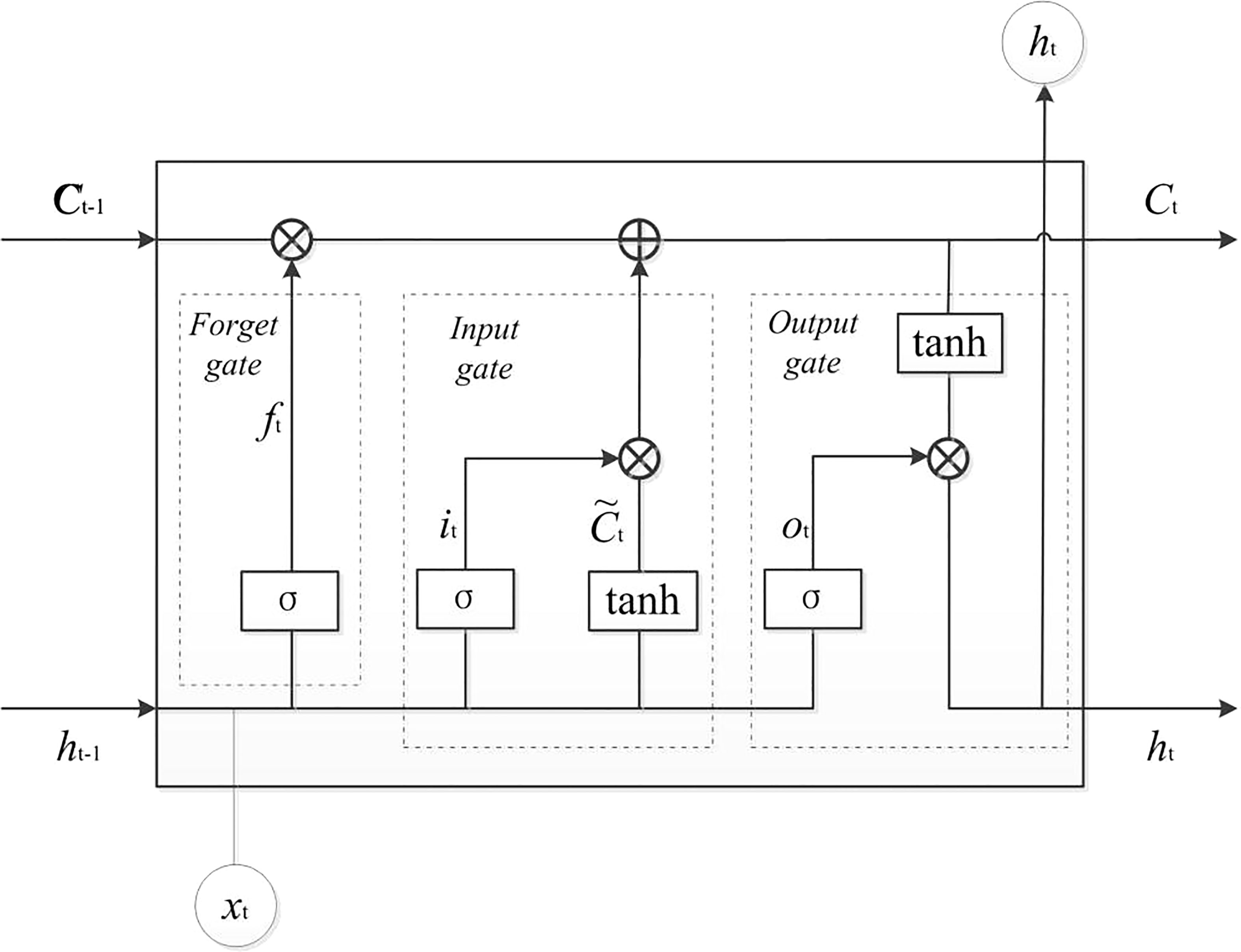
Figure 2 Structure of an LSTM cell.

$\begin{array}{ll}{f}_t=\sigma (W_f·[h_{t-1},x_t]+b_f)& (5)\end{array}$

$\begin{array}{ll}{i}_t=\sigma (W_i·[h_{t-1},x_t]+b_i)& (6)\end{array}$

$\begin{array}{ll}{\tilde{C}}_t=\text{tanh}(W_c·[h_{t-1},x_t]+b_C)& (7)\end{array}$

$\begin{array}{ll}{C}_t=f_t\ast C_{t-1}+i_t\ast {\tilde{C}}_t& (8)\end{array}$

$\begin{array}{ll}{o}_t=\sigma (W_o·[h_{t-1},x_t]+b_o)& (9)\end{array}$

$\begin{array}{ll}{h}_t=o_t\ast \tanh (C_t)& (10)\end{array}$

where f_t, i_t, and o_t represent the outputs of forget gate, input gate, and output gate, respectively. C_t is the cell state vector, and σ is the sigmoid function. W_f, W_i, Wo, and W_C are the corresponding weights; b_f, b_i, bo, and b_c are the corresponding biases. h_t is the output, ${\tilde{C}}_t$ is the new memory vector, and x_t is the input.

In this study, we build a 4-layer deep neural network model to conduct 120-day Kuroshio path prediction experiments based on the LSTM neural network. By trial and error, the size of the time window used to predict the Kuroshio path is set to 30, which means that we use the preceding 30-day Kuroshio path data for prediction. Besides, the adaptive moment estimation (Adam) is taken as the gradient optimization algorithm, which provides an optimized method for solving sparse gradients and noise problems (Song et al., 2020). The rectified linear unit (ReLU) function is used as the activation function. This function avoids the gradient vanishing problem of the sigmoid function and tanh function, and it has a high calculation efficiency.

2.2.4 Evaluation criteria

To evaluate the performance of the prediction models, we employ root-mean-square error (RMSE), anomaly correlation coefficient (ACC), and prediction skill score (SS) as the evaluation criteria. These calculation formulas are defined as follows:

$\begin{array}{ll}\text{RMSE}=\sqrt{\frac{{\displaystyle \sum _{j=1}^m{x}_{i,j}^P-x_{i,j}^T}}{m}}& (11)\end{array}$

$\begin{array}{ll}ACC=\frac{{\displaystyle \sum _{i=1}^n(x_{i,j}^P-{\overline{x}}_j^P)(x_{i,j}^T-{\overline{x}}_j^T)}}{\sqrt{{{\displaystyle \sum _{i=1}^n{(x_{i,j}^P-{\overline{x}}_j^P)}^2(x_{i,j}^T-{\overline{x}}_j^T)}}^2}}& (12)\end{array}$

$\begin{array}{ll}\text{SS}=1-\frac{\text{MSE}(p,o)}{\text{MSE}(c,o)}& (13)\end{array}$

where $x_{i,j}^P$ and $x_{i,j}^T$ are prediction and true values, respectively, of the Kuroshio path of the i^th grid point on the j^th day; . ${\overline{x}}_j^P={\displaystyle \sum _{i=1}^n{x}_{i,j}^P}$. and ${\overline{x}}_j^T={\displaystyle \sum _{i=1}^n{x}_{i,j}^T}$ are prediction and true mean values of the Kuroshio path on the j^th day, respectively;m is the number of days of testing data; n is the number of spatial grid points representing the Kuroshio path; RMSE is the root-mean-square error of the i^th grid point; and ACC is the spatial anomaly correlation coefficient of the j^th day. $\text{MSE}(p,o)=\frac{1}{m}{\displaystyle \sum _{j=1}^m{(x_{i,j}^P-x_{i,j}^T)}^2}$ denotes the mean square error between prediction and observations; $\text{MSE}(c,o)=\frac{1}{m}{\displaystyle \sum _{j=1}^m{(x_i^C-x_{i,j}^T)}^2}$denotes the mean square error between climatology and observations, in which $x_i^C$ is climatological value of the Kuroshio path of the i^th grid point.

3 Prediction experments

3.1 Comparison of EOF-LSTM and CEOF-LSTM models

First, we construct the CEOF-LSTM (EOF-LSTM) prediction model, based on the CEOF (EOF) analysis and LSTM neural network only (see Figure 6). To compare the performance from the CEOF analysis with the EOF analysis for the Kuroshio path prediction, we conduct 120-day Kuroshio path prediction experiments. After the CEOF (EOF) analysis, the Kuroshio path data are decomposed into several modes and separated into CEOFs (EOFs) and CPCs (PCs). To reduce the cost time, we use the first 16 CEOFs (18 EOFs) and their corresponding CPCs (PCs), accounting for 99% of the total variance, as input parameters to predict the CPC (PC) time series for different lead times. All the modes used pass the North significance test (North et al., 1982); and these CEOFs (EOFs) and CPCs (PCs) are able to reconstruct the main characteristics of the Kuroshio path. After training the model, the CPC (PC) time series of the significant Kuroshio path are predicted, and the Kuroshio paths are reconstructed by using these predicted CPCs (PCs) and the CEOFs (EOFs) from the CEOF (EOF) analysis. The residual from the unused higher-order modes of the CEOF (EOF) analysis (accounting for 1% of the total variance) at the start time serves as a correction to obtain the final prediction in a form of persistence. Such a correction can improve the prediction skill in the first three days of the lead time. Compared with the prediction experiment without the correction, the RMSEs of the CEOF-LSTM (EOF-LSTM) model prediction results are reduced by 12.2% (6.2%), 6.1% (2.7%), and 1.8% (0.7%), respectively; and the ACC values are increased by 0.0038 (0.0032), 0.0022 (0.0014), and 0.0007 (0.0007), respectively.

Figure 3 shows the averaged RMSE and ACC of the predictions for different lead times using CEOF-LSTM (red line) and EOF-LSTM (green line) models. The dashed black line indicates the climatological standard deviation of the 50-year (1958-2007) Kuroshio path. It can be seen that the RMSE of the CEOF-LSTM model is significantly smaller than that of the EOF-LSTM model for each lead time. The ACC of the CEOF-LSTM model is below 0.6 (the black dashed line in Figure 3B, which has the spatial ACC of 0.6, a thumb rule for measuring “usefulness” of predictions; Pendlebury et al., 2003) at the lead time of 100 days, while the ACC of the EOF-LSTM is below 0.6 as early as 35 days. When the lead time is 120 days, the RMSE of the CEOF-LSTM model is reduced by 12%, and the ACC is improved by 0.23 compared to the EOF-LSTM model.

FIGURE 3

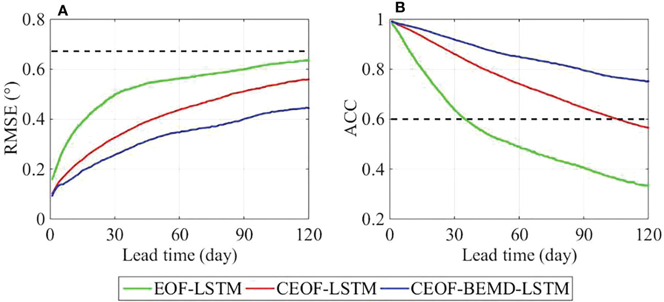
Figure 3 (A) Space-averaged RMSE (°) of the prediction using the EOF-LSTM, CEOF-LSTM, and CEOF-BEMD-LSTM models. The dashed black line indicates the climatological standard deviation of the Kuroshio path. (B) Averaged ACC values of the predictions using the EOF-LSTM, CEOF-LSTM, and CEOF-BEMD-LSTM models. The dashed black line indicates spatial ACC of 0.6, a thumb rule for measuring “usefulness” of predictions.

Figures 4A, C depict temporal-spatial distributions of RMSE for the 1-120 days Kuroshio path predictions using the EOF-LSTM and CEOF-LSTM models. The solid black contour indicates the prediction range where the RMSE at each location of the Kuroshio path reaches its climatological standard deviation. Both RMSEs exhibit similar spatial distributions, but the RMSE of the CEOF-LSTM model is smaller. To compare the RMSEs of these two models better, we also calculate the temporal-spatial distributions of difference between the RMSE of the CEOF-LSTM model and that of the EOF-LSTM model, as shown in Figure 5A. The RMSE of the CEOF-LSTM model is significantly smaller than that of the EOF-LSTM model in all regions, especially in the region of 137°-140°E. It can be reduced by as much as 0.3°.

FIGURE 4

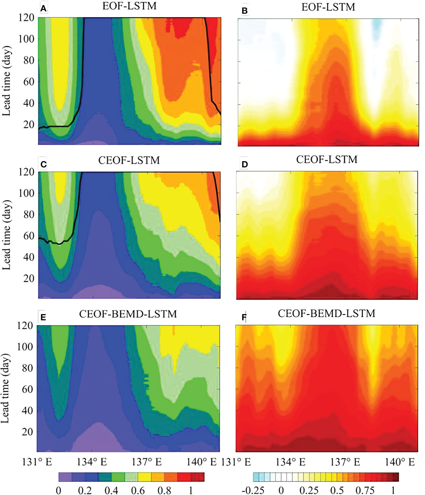
Figure 4 Left panels (A, C, E): Temporal-spatial distributions of RMSE (°) of the 1-120 days Kuroshio path predictions using EOF-LSTM, CEOF-LSTM, and CEOF-BEMD-LSTM models. The solid black contour indicates the prediction range where the RMSE at each location of the Kuroshio path reaches its climatological standard deviation. Right panels (B, D, F): Same as the left panels, except for temporal-spatial distributions of prediction skill score.

FIGURE 5

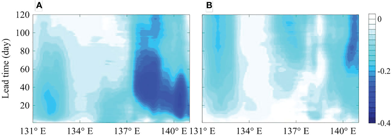
Figure 5 (A) Temporal-spatial distributions of difference between the RMSE of the CEOF-LSTM model and that of the EOF-LSTM model in the 1-120 days predictions. Negatives value means that the RMSE of the CEOF-LSTM model is smaller than that of the EOF-LSTM model. (B) Same as (A), except for the difference between the RMSE of CEOF-BEMD-LSTM model and that of the CEOF-LSTM model. Negatives value means that the RMSE of the CEOF-BEMD-LSTM model is smaller than that of the CEOF-LSTM model.

In summary, the CEOF analysis is significantly better than the EOF analysis for predicting the Kuroshio path south of Japan. It may be due to these following reasons: The CEOF analysis can resolve propagating wave signals (Bouzinac et al., 1998), which are closely related to the variation of the Kuroshio path, while the EOF analysis cannot reveal such signal characteristics. The LSTM neural network can capture and learn these signal features during the training process, and thus the prediction of the CEOF-LSTM model is better. Considering the comparison results and explanations above, we conduct further predictions based on the CEOF-LSTM model in the following-up experiments.

3.2 Prediction experiments using CEOF-BEMD-LSTM model

To improve the performance of the CEOF-LSTM model, we add the BEMD analysis to the prediction model (Rilling et al., 2007; Shao et al., 2021a), called the CEOF-BEMD-LSTM model. Figure 6 shows the framework of the CEOF-BEMD-LSTM model, which can be broken down into three parts: (A) data preprocessing, (B) LSTM prediction, and (C) correction. During the first part of data preprocessing, the Kuroshio path data are first divided into training dataset and testing dataset. Then, the CEOF analysis decomposes the training dataset into CEOFs and CPCs. The CPCs of the testing dataset are obtained by projecting the testing dataset onto the CEOFs. Next, the BEMD analysis is conducted on the first 16 CPCs (accounting for 99% of the total variance) to extract the CIMFs. Each CPC is decomposed into 16 CIMFs; and all the CIMFs serve as the inputs for the LSTM neural network. In the second part of LSTM prediction, the LSTM neural network is used to predict the CIMFs. After training and predicting, the predictions of the CPCs are obtained by using the predictions of the CIMFs, which are the outputs of the LSTM neural network. Based on the predictions of the CPCs and the CEOFs obtained from the CEOF analysis, the predictions of the Kuroshio path are reconstructed. In the last part of the correction, the final prediction is obtained by adding the residual, which consists of unused higher-order modes of the CEOF analysis (accounting for 1% of the total variance) at the start time, as a correction in a form of persistence. Similar to the results presented in section 3.1, the prediction skill in the first three days of the lead time is better than that of the prediction experiment without the correction. Specifically, the RMSEs of the prediction results are reduced by 14.2%, 6.4%, and 1.9%, respectively; and the ACC values are increased by 0.0038, 0.0023, and 0.0006, respectively.

FIGURE 6

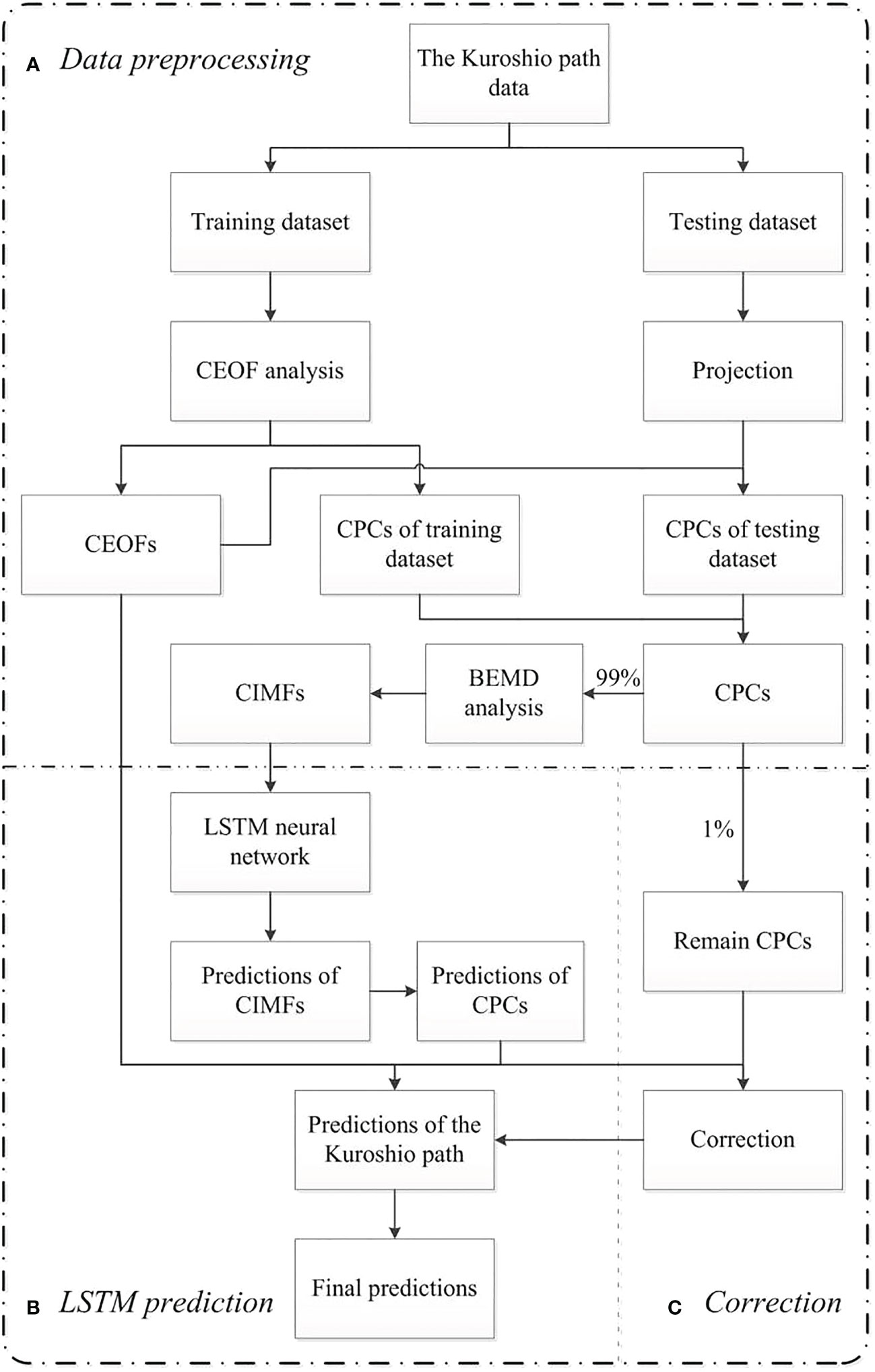
Figure 6 Framework of CEOF-BEMD-LSTM model.

In this section, we compare the predictions of the CEOF-BEMD-LSTM model with those of the CEOF-LSTM model to evaluate the performance of the CEOF-BEMD-LSTM model. Figure 3 shows the averaged RMSE and ACC values of the predictions for different lead times using the CEOF-LSTM (red line) and CEOF-BEMD-LSTM (blue line) models. The dashed black line indicates the climatological standard deviation of the 50-year (1958-2007) Kuroshio path. The RMSE of the CEOF-LSTM model is significantly larger than that of the CEOF-BEMD-LSTM model when the lead time is 120 days, and exceeding the climatological standard deviation of the Kuroshio path. Compared with the CEOF-LSTM model (red line), the performance of the CEOF-BEMD-LSTM model (blue line) exhibits better prediction results, with smaller RMSE and larger ACC (blue line). Even to 120 days, the RMSE of the CEOF-BEMD-LSTM model is much smaller than the climatological standard deviation of the Kuroshio path, and the ACC of the CEOF-BEMD-LSTM model exceeds 0.7. Compared with the CEOF-LSTM model, the RMSE of the CEOF-BEMD-LSTM model in the prediction results of day 120 is reduced by 26%, and the ACC is improved by 0.19.

Figures 4C, E show temporal-spatial distributions of RMSE for the 1-120 days Kuroshio path prediction results using the CEOF-LSTM and CEOF-BEMD-LSTM models. The solid black contour indicates the prediction range, where the RMSE of each location of the Kuroshio path achieves its climatological standard deviation. The RMSEs of both models expand progressively with increasing lead time; and the RMSEs of both models in the Kuroshio large meander region gradually converge downstream and attain their maxima in the Izu-Ogasawara Ridge (IOR) region with the same lead time. This is probably because the Kuroshio path in this region changes frequently, leading to lower signal-to-noise ratios and larger errors for the predictions. More importantly, the prediction range of the CEOF-BEMD-LSTM model exceeds 120 days (Figure 4E), while the prediction ranges of the CEOF-LSTM model are under 120 days in the upper Kuroshio (131°-135°E) and IOR (Figures 4C) and their RMSEs are larger. We also depict the temporal-spatial distributions of the difference between the RMSE of the CEOF-BEMD-LSTM model and that of the CEOF-LSTM model in the 1-120 days predictions. Figure 5B clearly shows that the RMSE of the CEOF-BEMD-LSTM model is smaller than that of the CEOF-LSTM model in all locations.

We also calculate the prediction skill score (SS) with each model to further evaluate the predictions. The SS is positive (negative) when the accuracy of the prediction is greater (less) than the accuracy of the climatology (Murphy, 1988). Meanwhile, the closer the SS approaches toward 1, the better the prediction. The temporal-spatial distributions of SS for the 1-120 days Kuroshio path predictions using the EOF-LSTM, CEOF-LSTM, and CEOF-BEMD-LSTM models are described in the right panels of Figure 4. The SSs of all models show similar distributions. Specially, the SSs decrease gradually as the lead time increases. They are larger in the 135°-138°E region and gradually decrease to the east and west (Figures 4D, F). Moreover, the CEOF-BEMD-LSTM model demonstrates the best SS. When the lead time is 120 days, the SS of this model is still maintained above 0.3, being larger than other models’. In the meanwhile, the SS remains relatively high in the IOR despite the large RMSE in the region. To summarize, the CEOF-BEMD-LSTM model exhibits the best prediction skill in the 120-day Kuroshio path prediction experiments.

3.3 The latest Kuroshio large meander prediction

The latest Kuroshio large meander occurred in August 2017, and is the second Kuroshio large meander in this century. As a unique phenomenon, the Kuroshio large meander has a significant impact on climate change along the southern coast of Japan (Sugimoto et al., 2020; Sugimoto et al., 2021). Therefore, Kuroshio large meander prediction is one of the important goals to conduct the experiments for predicting the Kuroshio path south of Japan. Considering the best performance of the CEOF-BEMD-LSTM model presented in section 3.2, we use the CEOF-BEMD-LSTM model to predict the latest Kuroshio large meander next.

Figure 7 depicts the predictions of the Kuroshio path with the lead time of 120 days from July 1 (1-day) to October 28 (120-day), 2017. In general, the Kuroshio large meander transforms from the nearshore non-large meander. However, this one switched from the offshore non-large meandering path (Figure 7A), accompanied by a smaller meander in the IOR. Then, the smaller meander continued to be advected downstream with decreasing amplitude and eventually disappeared (Figures 7B, C). Meanwhile, a trigger meander from upstream was advected to the southern sea of Honshu with increasing amplitude, eventually forming a stable Kuroshio large meander path (Figures 7D–I). Overall, the predicted Kuroshio path captures this process, namely, which implies that the Kuroshio path prediction with the CEOF-BEMD-LSTM model can predict the latest Kuroshio large meander formation process. Noted that the prediction errors exist within the region of Kuroshio large meanders and the prediction magnitude is smaller than the actual Kuroshio path (Figures 7C–I).

FIGURE 7

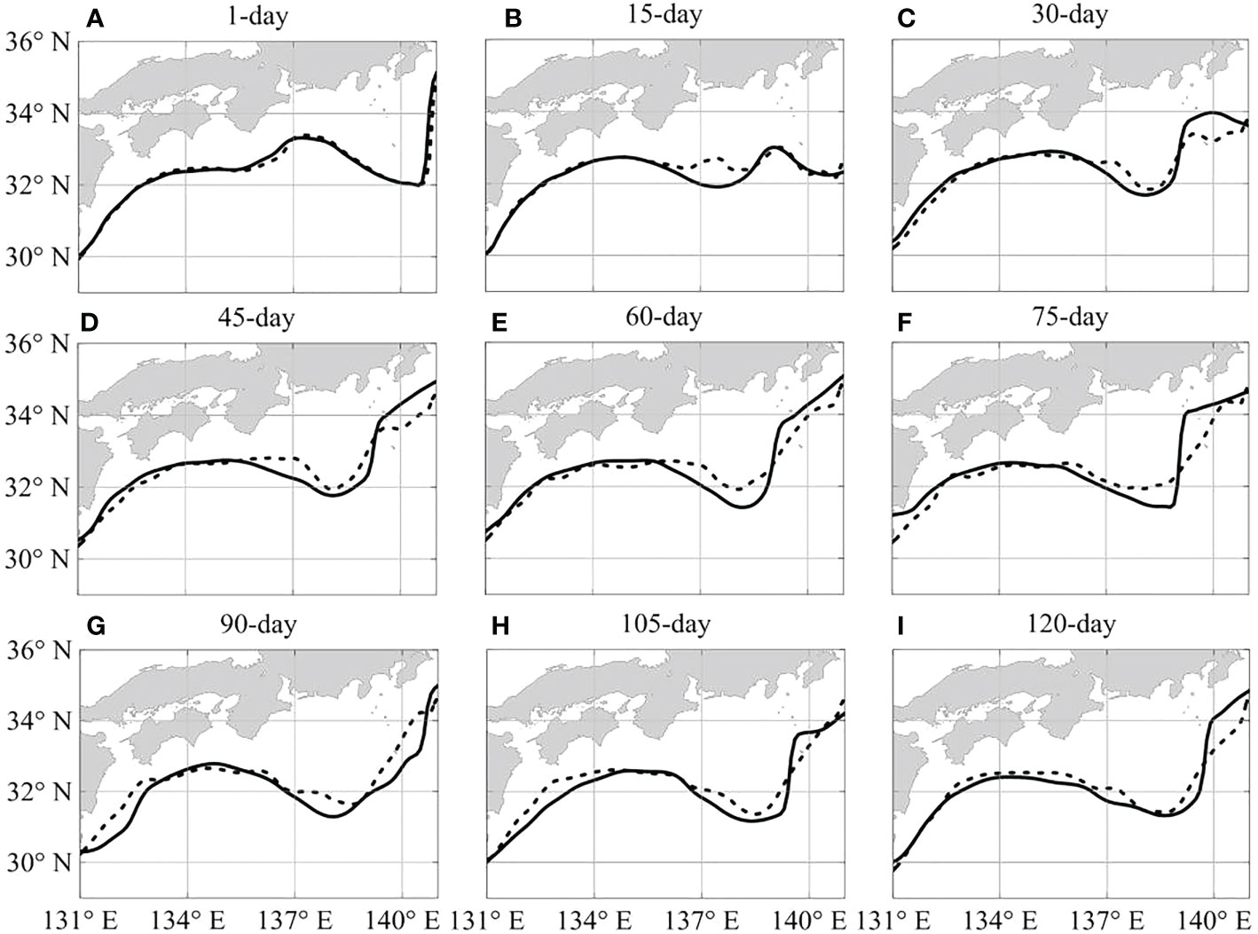
Figure 7 Prediction results of the Kuroshio path with the lead time of 120 days from July 1 (1-day) to October 28 (120-day), 2017 (A–I). The solid curve represents the true path, and the dashed one represents the prediction.

The latest Kuroshio large meander has lasted for five years and remains so. In the final part of this section, we use the CEOF-BEMD-LSTM model to predict the Kuroshio path south of Japan for 120 days from January 1 (1-day) to April 30 (120-day), 2023. The prediction results indicate that the Kuroshio will remain in the state of the large meander (Figure 8). The position of the large meander will gradually shift westward from 137.4°E on January 1, 2023 (dashed red line) to 136.5°E on April 30, 2023 (dashed brown line).

FIGURE 8

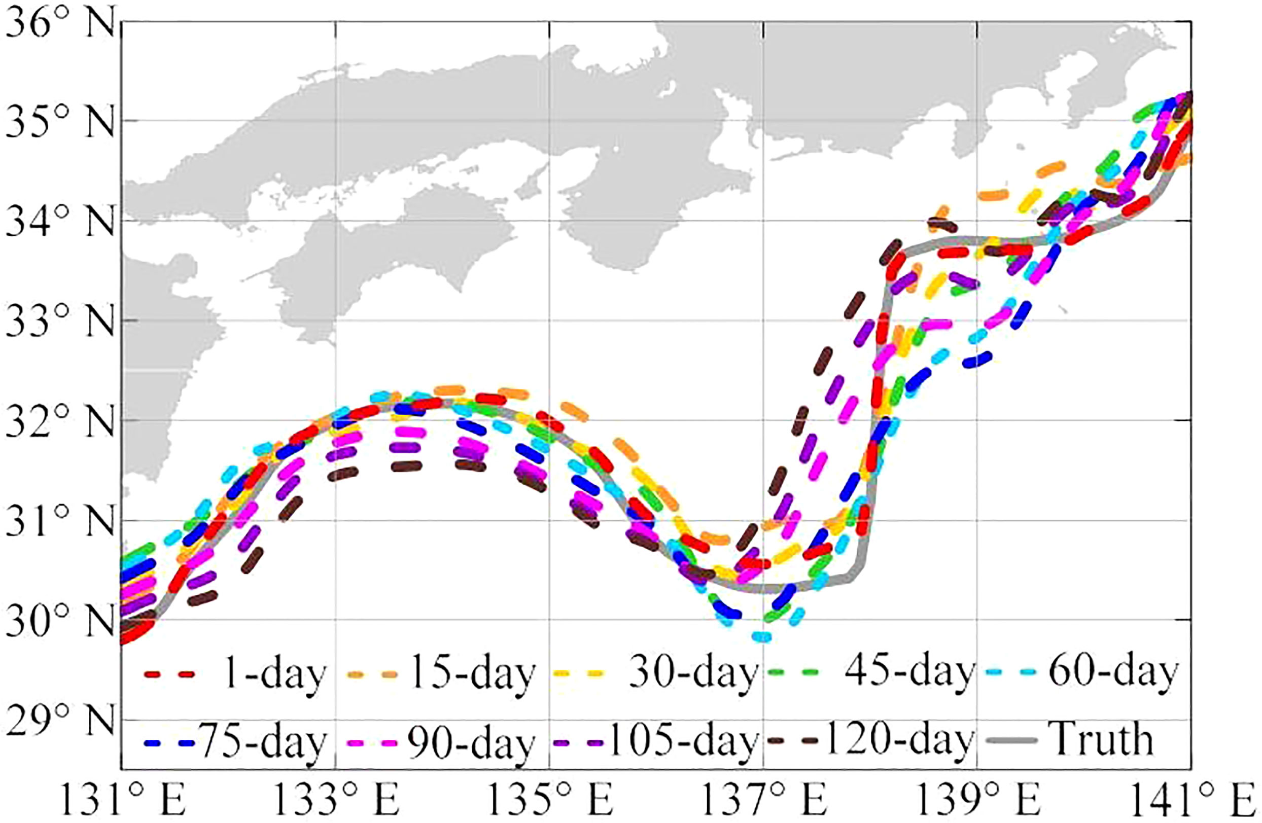
Figure 8 Prediction results of the Kuroshio path with the lead time of 120 days from January 1 (1-day) to April 30 (120-day), 2023. The solid gray curve represents the truth at lead-time of one day.

4 Summary and discussion

In this study, a hybrid deep learning prediction model, called CEOF-BEMD-LSTM model, is developed for predicting the Kuroshio path south of Japan based on the CEOF analysis, BEMD analysis, and LSTM neural network. To evaluate the performance of this model, we use the Kuroshio path data obtained from the CORA reanalysis dataset from 1958 to 2007 (50 years) as a training dataset, and its counterpart from the altimetry data from 2008 to 2022 as a testing dataset, to conduct 120-day Kuroshio path prediction experiments. Prediction results show that the CEOF-BEMD-LSTM model has good performance in the 120-day prediction range evaluated by using two common deterministic skill metrics, the ACC and RMSE. Even when the lead time is 120 days, the RMSE is about 0.44°, which is less than the climatological standard deviation, and the ACC can still reach 0.75, which is greater than 0.6 (a widely used measure for forecast verification; Pendlebury et al., 2003). This model also exhibits a good prediction skill score (SS). Besides, the model successfully hindcasts the formation of the latest Kuroshio large meander since the summer of 2017. Finally, we predict the Kuroshio path from January 1 to April 30, 2023, and the predictions indicate that the Kuroshio will continue to be a large meander.

Comparatively speaking, the prediction range of the traditional numerical prediction is usually 60 days (Komori et al., 2003; Miyazawa et al., 2005; Usui et al., 2006). At present, the JCOPE operational system provides the prediction of the Kuroshio path south of Japan with a two-month lead time (https://fra-roms.fra.go.jp/fra-roms/). However, since its predictions are given in figures with no statistics of the prediction results available, we cannot compare our results with theirs quantitatively. Currently, its two-month predictions show that the Kuroshio will continue to be a large meander, as our model does.

Some recent studies showed that the inclusion of appropriate predictors can improve the prediction range of deep learning models (e.g., Oh and Suh, 2018; Liang et al., 2021). In future research, great effort is required to seek predictor(s) of the Kuroshio path south of Japan, which should be encoded in a reasonable way.

Data availability statement

Publicly available datasets were analyzed in this study. This data can be found here: http://www.cmoc-china.cn/pages/productService.html https://resources.marine.copernicus.eu/product-detail/SEALEVEL_GLO_PHY_L4_NRT_OBSERVATIONS_008_046/DATA-ACCESS https://resources.marine.copernicus.eu/product-detail/SEALEVEL_GLO_PHY_L4_MY_008_047/DATA-ACCESS.

Author contributions

XW and ZJ constructed the prediction model and conducted the prediction experiments. XW wrote the initial draft and revised the manuscript. GH and WL proposed the main ideas and revised the manuscript. LC and WD provided high-performance data processing and revised the manuscript. All authors contributed to the article and approved the revised version.

Funding

This research is sponsored by the National Natural Science Foundation of China (grant 41876014).

Acknowledgments

The authors thank the following data and tool providers: the National Marine Data and Information Service (http://www.cmoc-china.cn) for providing the daily CORA dataset, the Copernicus Marine and Environment Monitoring Service for providing the altimetry dataset (https://resources.marine.copernicus.eu), Google for providing the open source machine learning framework TensorFlow (https://www.tensorflow.org/), Keras (https://keras.io/) for conducting deep learning prediction experiments, and Scikit-learn (http://scikit-learn.org/stable/) for providing the machine learning library based on which the experiments are conducted. The authors sincerely appreciate the reviewers for their valuable comments and suggestions on improving the quality of this paper.

Conflict of interest

The authors declare that the research was conducted in the absence of any commercial or financial relationships that could be construed as a potential conflict of interest.

Publisher’s note

All claims expressed in this article are solely those of the authors and do not necessarily represent those of their affiliated organizations, or those of the publisher, the editors and the reviewers. Any product that may be evaluated in this article, or claim that may be made by its manufacturer, is not guaranteed or endorsed by the publisher.

References

Bouzinac C., Vazquez J., Font J. (1998). Complex empirical orthogonal functions analysis of ERS-1 and TOPEX/POSEIDON combined altimetric data in the region of the Algerian current. J. Geophys. Res.-Oceans 103 (C4), 8059–8071. doi: 10.1029/97JC02909

CrossRef Full Text | Google Scholar

Ezer T., Mellor G. L. (2004). A generalized coordinate ocean model and a comparison of the bottom boundary layer dynamics in terrain-following and in z-level grids. Ocean Model. 6 (3-4), 379–403. doi: 10.1016/s1463-5003(03)00026-x

CrossRef Full Text | Google Scholar

Han G., Li W., Zhang X., Wang X., Wu X., Fu H., et al. (2013). A new version of regional ocean reanalysis for coastal waters of China and adjacent seas. Adv. Atmos. Sci. 30 (004), 974–982. doi: 10.1007/s00376-012-2195-4

CrossRef Full Text | Google Scholar

Hannachi A., Jolliffe I. T., Stephenson D. B. (2007). Empirical orthogonal functions and related techniques in atmospheric science: a review. Ini. J. Climatol. 27, 1119–1152. doi: 10.1002/joc.1499

CrossRef Full Text | Google Scholar

Hochreiter S., Schmidhuber J. (1997). Long short-term memory. Neural Computation. 9 (8), 1735–1780. doi: 10.1162/neco.1997.9.8.1735

PubMed Abstract | CrossRef Full Text | Google Scholar

Huang N. E., Shen Z., Long S. R., Wu M. C., Shih H. H., Zheng Q., et al. (1998). The empirical mode decomposition and the Hilbert spectrum for nonlinear and non-stationary time series analysis. Proc. R. Soc. London Ser. A-Mathemat. Phys. Sci. 454, 903–995. doi: 10.1098/rspa.1998.0193

CrossRef Full Text | Google Scholar

Kamachi M., Kuragano T., Sugimoto S., Yoshita K., Sakurai T., Nakano T., et al. (2004). Short-range prediction experiments with operational data assimilation system for the Kuroshio south of Japan. J. Oceanogr. 60, 269–282. doi: 10.1023/B:JOCE.0000038333.97882.51

CrossRef Full Text | Google Scholar

Kawabe M. (1995). Variations of current path, velocity, and volume transport of the Kuroshio in relation with the large meander. J. Phys. Oceanogr. 25, 3103–3117. doi: 10.1175/1520-0485(1995)025,3103:VOCPVA.2.0.CO;2

CrossRef Full Text | Google Scholar

Komori N., Awaji T., Ishikawa Y., Kuragano T. (2003). ). short-range forecast experiments of the Kuroshio path variabilities south of Japan using TOPEX/Poseidon altimetric data. J. Geophys. Res.-Oceans 108 (C1), 3010. doi: 10.1029/2001JC001282

CrossRef Full Text | Google Scholar

Liang X. S., Xu F., Rong Y., Zhang R., Tang X., Zhang F. (2021). El Niño modoki can be mostly predicted more than 10 years ahead of time. Sci. Rep. 11 (1), 17860. doi: 10.1038/s41598-021-97111-y

PubMed Abstract | CrossRef Full Text | Google Scholar

Liu J., Zhang T., Han G., Gou Y. (2018). TD-LSTM: Temporal dependence-based LSTM networks for marine temperature prediction. Sensors 18 (11), 3797. doi: 10.3390/s18113797

PubMed Abstract | CrossRef Full Text | Google Scholar

Li W., Xie Y., He Z., Han G., Liu K., Ma J., et al. (2008). Application of the multigrid data assimilation scheme to the China seas’ temperature forecast. J. Atmos. Oceanic Technol. 25 (11), 2106–2116. doi: 10.1175/2008JTECHO510.1

CrossRef Full Text | Google Scholar

Ma Y., Li G., Wang Y., Zhou H., Zhang B. (2015). Random noise attenuation by f-x spatial projection-based complex empirical mode decomposition predictive filtering. Appl. Geophys. 12, 47–54. doi: 10.1007/s11770-015-0467-3

CrossRef Full Text | Google Scholar

Mellor G. L., Häkkinen S. M., Ezer T., Patchen R. C. (2002). “A generalization of a sigma coordinate ocean model and an intercomparison of model vertical grids,” in Ocean forecasting. Eds. Pinardi N., Woods J. (Berlin, Heidelberg: Springer), 55–72. doi: 10.1007/978-3-662-22648-3_4

CrossRef Full Text | Google Scholar

Miyazawa Y., Kagimoto T., Guo X., Sakuma H. (2008). The Kuroshio large meander formation in 2004 analyzed by an eddy-resolving ocean forecast system. J. Geophys. Res.-Oceans. 113, C10015. doi: 10.1029/2007JC004226

CrossRef Full Text | Google Scholar

Miyazawa Y., Yamane S., Guo X., Yamagata T. (2005). Ensemble forecast of the Kuroshio meandering. J. Geophys. Res.-Oceans. 110, C10026. doi: 10.1029/2004JC002426

CrossRef Full Text | Google Scholar

Miyazawa Y., Zhang R., Guo X., Tamura H., Ambe D., Lee J. S. (2009). Water mass variability in the western north pacific detected in a 15-year eddy resolving ocean reanalysis. J. Oceanogr. 65 (6), 737–756. doi: 10.1007/s10872-009-0063-3

CrossRef Full Text | Google Scholar

Murphy A. H. (1988). Skill scores based on the mean square error and their relationships to the correlation coefficient. Mon. Wea. Rev. 116 (12), 2417–2424. doi: 10.1175/1520-0493(1988)116<2417:SSBOTM>2.0.CO;2

CrossRef Full Text | Google Scholar

Nakata H., Funakoshi S., Nakamura M. (2000). Alternating dominance of postlarval sardine and anchovy caught by coastal fishery in relation to the Kuroshio meander in the enshu-nada Sea. Fish. Oceanogr. 9 (3), 248–258. doi: 10.1046/j.1365-2419.2000.00140.x

CrossRef Full Text | Google Scholar

North G. R., Bell T. L., Cahalan R. F., Moeng F. J. (1982). Sampling errors in the estimation of empirical orthogonal functions. Mon. Wea. Rev. 110 (7), 699–706. doi: 10.1175/1520-0493(1982)110<0699:SEITEO>2.0.CO;2

CrossRef Full Text | Google Scholar

Oh J., Suh K. D. (2018). Real-time forecasting of wave heights using EOF-wavelet-neural network hybrid model. Ocean engineering. 150, 48–59. doi: 10.1016/j.oceaneng.2017.12.044

CrossRef Full Text | Google Scholar

Pendlebury S. F., Adams N. D., Hart T. L., Turner J. (2003). Numerical weather prediction model performance over high southern latitudes. Mon. Wea. Rev. 131 (2), 335–353. doi: 10.1175/1520-0493(2003)131<0335:NWPMPO>2.0.CO;2

CrossRef Full Text | Google Scholar

Qiu B., Chen S., Schneider N., Oka E., Sugimoto S. (2021). On reset of the wind-forced decadal Kuroshio extension variability in late 2017. J. Climate. 33 (24), 10813–10827. doi: 10.1175/JCLI-D-20-0237.1

CrossRef Full Text | Google Scholar

Reichstein M., Camps-Valls G., Stevens B., Jung M., Denzler J., Carvalhais N., et al. (2019). Deep learning and process understanding for data-driven earth system science. Nature 566, 195–204. doi: 10.1038/s41586-019-0912-1

PubMed Abstract | CrossRef Full Text | Google Scholar

Rilling G., Flandrin P., Goncalves P., Lilly J. M. (2007). Bivariate empirical mode decomposition. IEEE Signal Process. Lett. 14 (12), 936–939. doi: 10.1109/LSP.2007.904710

CrossRef Full Text | Google Scholar

Shao Q., Hou G., Li W., Han G., Liang K., Bai Y. (2021a). Ocean reanalysis data-driven deep learning forecast for sea surface multivariate in the South China Sea. Earth Space Sci. 8, e2020EA001558. doi: 10.1029/2020EA001558

CrossRef Full Text | Google Scholar

Shao Q., Li W., Han G., Hou G., Liu S., Gong Y., et al. (2021b). A deep learning model for forecasting sea surface height anomalies and temperatures in the South China Sea. J. Geophys. Res.-Oceans. 126, e2021JC17515. doi: 10.1029/2021JC017515

CrossRef Full Text | Google Scholar

Song T., Jiang J., Li W., Xu D. (2020). A deep learning method with merged LSTM neural networks for SSHA prediction. IEEE J-STARS. 13, 2853–2860. doi: 10.1109/JSTARS.2020.2998461

CrossRef Full Text | Google Scholar

Sugimoto S., Qiu B., Kojima A. (2020). Marked coastal warming off Tokai attributable to Kuroshio large meander. J. Oceanogr. 76 (2), 141–154. doi: 10.1007/s10872-019-00531-8

CrossRef Full Text | Google Scholar

Sugimoto S., Qiu B., Schneider N. (2021). Local atmospheric response to the Kuroshio large meander path in summer and its remote influence on the climate of Japan. J. Climate. 34 (9), 3571–3589. doi: 10.1175/JCLI-D-20-0387.1

CrossRef Full Text | Google Scholar

Tsujino H., Usui N., Nakano H. (2006). Dynamics of Kuroshio path variations in a high-resolution general circulation model. J. Geophys. Res.-Oceans. 111, C11001. doi: 10.1029/2005JC003118

CrossRef Full Text | Google Scholar

Usui N., Nagai T., Saito H., Suzuki K., Takahashi M. (2019). Progress of studies on Kuroshio path variations south of Japan in the past decade, in the Kuroshio current: physical, biogeochemical, and ecosystem dynamic, Vol. 9. Eds. Nagai T., Saito H., Suzuki K., et al, American Geophysical Union (AGU). 147–161. doi: 10.1002/9781119428428.ch9

CrossRef Full Text | Google Scholar

Usui N., Tsujino H., Fujii Y., Kamachi M. (2006). Short-range prediction experiments of the Kuroshio path variabilities south of Japan. Ocean Dynam. 56, 607–623. doi: 10.1007/s10236-006-0084-z

CrossRef Full Text | Google Scholar

Wu X., Zhao Y., Han G., Li W., Shao Q., Cao L., et al. (2022). Temporal-spatial oceanic variation in relation with the three typical Kuroshio paths South of Japan. Acta Oceanol. Sin. 41 (2), 15–25. doi: 10.1007/s13131-021-1941-9

CrossRef Full Text | Google Scholar

Xiao C., Chen N., Hu C., Wang K., Gong J., Chen Z. (2019). Short and mid-term sea surface temperature prediction using time-series satellite data and LSTM-AdaBoost combination approach. Remote Sens. Environ. 233, 111358. doi: 10.1016/j.rse.2019.111358

CrossRef Full Text | Google Scholar

Yang Y., Liang X. S. (2019). New perspectives on the generation and maintenance of the Kuroshio large meander. J. Phys. Oceanogr. 49 (8), 2095–2113. doi: 10.1175/JPO-D-18-0276.1

CrossRef Full Text | Google Scholar