Inversion of shallow seabed structure and geoacoustic parameters with waveguide characteristic impedance based on Bayesian approach

Underwater acoustic technology is essential for ocean observation, exploration and exploitation, and its development is based on an accurate predication of underwater acoustic wave propagation. In shallow sea environments, the geoacoustic parameters, such as the seabed structure, the sound speeds, the densities, and the sound speed attenuations in seabed layers, would significantly affect the acoustic wave propagation characteristics. To obtain more accurate inversion results for these parameters, this study presents an inversion method using the waveguide characteristic impedance based on the Bayesian approach. In the inversion, the vertical waveguide characteristic impedance, which is the ratio of the pressure over the vertical particle velocity, is set as the matching object. The nonlinear Bayesian theory is used to invert the above geoacoustic parameters and analysis the uncertainty of the inversion results. The numerical studies and the sea experiment processing haven shown the validity of this inversion method. The numerical studies also proved that the vertical waveguide characteristic impedance is more sensitive to the geoacoustic parameters than that of single acoustic pressure or single vertical particle velocity, and the error of simulation inversion is within 3%. The sea experiment processing showed that the seabed layered structure and geoacoustic parameters can be accurately determined by this method. The root mean square between the vertical waveguide characteristic impedance and the measured impedance is 0.38dB, and the inversion results accurately represent the seabed characteristics in the experimental sea area.

1. Introduction

At present, using acoustic waves is the only method for detecting over long distances in seawater (Zhang et al., 2020; Miao et al., 2021a; Miao et al., 2021b). Underwater acoustic technology has become indispensable ocean observation, exploration, and exploitation (Xing et al., 2021; Zhang et al., 2021; Rong and Xu, 2022). The development of underwater acoustic technology is based on accurate prediction of underwater acoustic wave propagation (Zhou et al., 2021).

In the shallow seas, the structure and geoacoustic parameters of the seabed significantly affect underwater acoustic propagation (Guo et al., 2017; Yu et al., 2022). The geoacoustic parameters in each seabed layer, such as sound speeds, density and attenuations, all have significant effects on the underwater acoustic field prediction, the sonar performance prediction, the underwater acoustic detection and the underwater acoustic communication (Zhang et al., 2022; Zhao et al., 2022). Therefore, the acquisition of geoacoustic parameters is particularly important in shallow sea (Zhang et al., 2019; Yang et al., 2020). Although, the geoacoustic parameters can be obtained by direct core sample measurements, it is very time consuming and costly to obtain enough samples for a large area. Acoustic waves can propagate rapidly over a large area and carry amounts of information about the shallow seabed, requiring estimation of geoacoustic parameters.

In recent years, several studies have been conducted to derive geoacoustic parameters from shallow sea acoustic data. In these studies, the geoacoustic parameters could be inverted by matching the propagation characteristics of the acoustic waves with replicates from the acoustic computational model. As a results, the geoacoustic parameters inversion method was proposed (Yang et al., 2020). Hermand (Hermand, 1999) investigated an inversion method to rapidly estimate the distribution of seabed acoustic features using a controlled source and a single hydrophone. In the acoustic parameter inversion experiment conducted by the Chinese Academy of Sciences, the seabed sound speed and attenuation coefficient of the seabed were determined based on using the pulse waveform and transimission loss (Li et al., 2000). Park et al. (Park et al., 2005) used the time-domain waveform received from a towed array to invert the geoacoustic parameters, the inversion result is consistent with the previous measurementresults in the same sea area. By matching the acoustic pressure field excited with a point source, Zheng et al. (Zheng et al., 2021) studied a Bayesian inversion method for geoacoustic parameters in a shallow sea. However, the above inversion methods all belong to active inversion, which primarily uses the acoustic pressure field as the match object, which is actively excited by a point acoustic source. Recent research shows that, in a shallow sea, the acoustic pressure field lacks some acoustic field information, and resulting in its insensitivity to some geoacoustic parameters, which causes it to be insensitive to some geoacoustic parameters, reducing the accuracy of the inversion results. From the persoective of environmental protection, it is better to use passive acoustics inversion from the sources of opportunity in the propagation medium (Ren and Hermand, 2013; Li et al., 2019; Li et al., 2022). These sources of chance, such as ship noise, sea noise, and marine animal sounds, are widely distributed in shallow seas. However, their unknown propagation characteristics, appearances, and durations make passive inversion considerably more difficult than active inversion. With the advent of acoustic vector sensors, they have provided ideas for the development of passive inversion methods (Zhang et al., 2010).

Acoustic vector sensors can simultaneously measure the scalar acoustic field and the vector gradient field (first order as vector velocity field, or second order as acceleration field), which can contain more information about the acoustic field suitable for passive geoacoustic inversion (Sun et al., 2020). Geoacoustic parameters inversion using acoustic vector sensors has been a hot topic in the last decade.(Huang et al, 2010; Dahl et al, 2022). Santos et al. achieved a reliable estimation of seabed parameters using high-frequency signals and a small aperture vertical vector sensor array (Santos et al., 2009). Sun and Li (Sun et al., 2013) used a vector sensor array to invert the geoacoustic parameters, and effectively reduce the estimation range of seabed sound speed. Zhu et al. compared the acoustic pressure, the vertical particle velocity, and the vertical waveguide characteristic impedance for each geoacoustic parameter of a shallow seabed. The results showed that the waveguide characteristic impedance was more sensitive to changes in the geoacoustic parameters (Zhu et al., 2015). Dahl used automatic vector recorders to record ship noise and then estimated the seabed characteristics using them (Dahl and Dall'Osto, 2020). All of the above studies prove that the research on geoacoustic parameters inversion using vector sensors is beneficial, and the combinations of scalar and vector fields are more suitable for passive geoacoustic parameters inversion. However, in the current inversion research, most studies only considered the effect of seabed compression-wave (P-wave) speed, that is, the seabed is preset as a single-layer liquid seabed model, and the layered structure of the seabed is ignored. It is still a challenge to determine the seabed structure and the geoacoustic parameters of each seabed layer simultaneously (Ren et al., 2018; Kavoosi et al., 2021).

When analyzing inversion results, existing researches has focused on the optimal solution under specific conditions. Because geoacoustic parameter inversion is a complex, multidimensional, nonlinear optimization problem, the uncertainty analysis of inversion results is also vital. Uncertainty analysis of the results can be performed using the Bayesian approach to inversion (Tollefsen and Dosso, 2020). The Bayesian method combines prior information from the model with the measured dataset. It performs quantitative statistical analysis of the inversion results of parameters, and expresses the posterior probability density (PPD) of the inversion results. The Bayesian information criterion (BIC) can also determine the optimal model that fully explains the observed data using different parameterizations (Dosso et al., 2017).

To obtain more accurate inversion results, this study presents an inversion method with waveguide characteristic impedance based on the Bayesian approach. In an inversion, the vertical waveguide characteristic impedanceis set as the match object, and the Bayesian theory is used to invert the seabed structure, the sound speeds, the densities and the sound speed attenuations in seabed layers. We anticipate that these research results will enrich existing applications of acoustic vector sensor and can be used to develop an effective inversion method for geoacoustic parameters in complex shallow sea environments.

The remainder of this paper is organized as follows. Section 2 and Section 3 present the waveguide characteristic impedancein shallow sea and the proposed Bayesian inversion method are introduced in Section 2 and Section 3, respectively. Section 4 dicusses the advantages of the waveguide characteristic impedance in geoacoustic inversion and reviews the effectiveness of the proposed inversion method is verified also in this section. Section 5 describes the application of theproposed method using ship-radiated noise data measured in the Dalian Sea area. Finally, the conclusions are summarized in Section 6.

2. Modeling of waveguide characteristic impedance

Considering the influence of seabed shear-wave (S-wave) speed on acoustic propagation in a shallow sea cannot be ignored (Zhu et al., 2015). In this study, the characteristics of the shallow seabed were regarded as a semi-infinite elastic seabed covered with a uniform horizontal layered medium with multiple elastic sediments (Zheng et al., 2020). The modeling is performed assuming N×2D in a cylindrical coordinate system. Ignoring the mutual coupling of acoustic waves between the two-dimensional vertical planes in the θ direction, in the (r, z) plane, set z=0 to represents the sea surface, the downward sea surface is the direction of the positive value of the depth z-axis, and the positive r-axis represents the acoustic field propagation direction. A schematic representation of the model is shown in Figure 1.

FIGURE 1

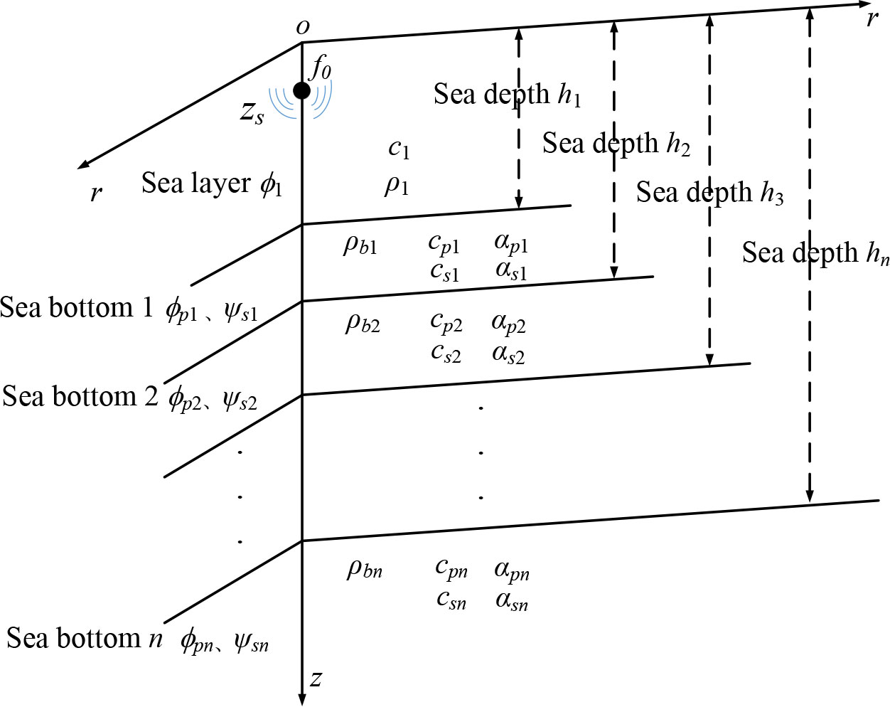
Figure 1 The shallow water environment model with an n-layered elastic seabed.

As shown in Figure 1, the depth of the sea layer is set as h₁, the sound source with frequency f₀ is located at the depth of the seawater layer z_s, and the density and the sound speed in the layer are ρ₁ and c₁, respectively. The density, compression-wave (P-wave) speed, S-wave speed, P-wave speed attenuation, S-wave speed attenuation, and layer thickness of the seabed layers are represented by ρ_bn, c_pn, c_sn, α_pn, α_sn and h_n, respectively. These above parameters are the seabed geoacoustic parameters to be inverted in this study.

In the context of the acoustic wave theory, the physical quantities in the model can be represented by the displacement potential function. Setting thedisplacement potential function in the seawater layer is ϕ₁, it satisfies the wave equation as follows:

$\begin{array}{ll}\frac{1}{r}\frac{\partial }{\partial r}\left(r\frac{\partial {\varphi }_1}{\partial r}\right)+\frac{{\partial }^2{\varphi }_1}{\partial z^2}+k_1^2{\varphi }_1=-4\pi \delta (r,z-z_s)0\le z\le h_1& (1)\end{array}$

its formal solution is

$\begin{array}{ll}{\varphi }_1(r,z,\omega )={\displaystyle \underset{0}{\overset{\infty }{\int }}{Z}_1(z,\xi ,\omega )J_0(\xi r)\xi \text{d}\xi }& (2)\end{array}$

where Z₁ is the ordinary differential equation of depth z and horizontal wavenumber ξ, and J₀ is the zero-order Bessel function. A detailed theoretical derivation can be found in the literature (Zhu et al., 2020).

The acoustic pressure field p, and the particle velocity field v can be expressed as follows:

$\begin{array}{ll}p(r,z,\omega )={\rho }_1{\omega }^{2}S\left(\omega \right){\varphi }_1={\rho }_1{\omega }^{2}S\left(\omega \right){\displaystyle \underset{0}{\overset{\infty }{\int }}{Z}_1(z,\xi ,\omega )J_0(\xi r)\xi d\xi }& (3)\end{array}$

$\begin{array}{ll}\mathbf{\text{v}}(r,z,\omega )=\{\begin{array}{c}{v}_r(r,z,\omega )=-i\omega S\left(\omega \right)\frac{\partial {\varphi }_1}{\partial r}=i\omega S\left(\omega \right){\displaystyle \underset{0}{\overset{\infty }{\int }}{Z}_1(z,\xi ,\omega ){\text{J}}_0(\xi r){\xi }^2\text{d}\xi }\\ v_z(r,z,\omega )=-i\omega S\left(\omega \right)\frac{\partial {\varphi }_1}{\partial z}=-i\omega S\left(\omega \right){\displaystyle \underset{0}{\overset{\infty }{\int }}\frac{\partial \left[Z_1(z,\xi ,\omega )\right]}{\partial z}{J}_0(\xi r)\xi d\xi }\end{array}& (4)\end{array}$

S(ω) represents the source level at f₀.

In general, the normal mode method (NMM) and the fast field method (FFM) can be used to solve Equation (3) and Equation (4) for the shallow sea environment, FFM converts the integral formula in the two equations into the form of Fourier transform and solved directly, it is more suitable for the rapid calculation of shallow sea acoustic field (Zhu et al., 2020). Therefore, in this study, the FFM is selected for solving the above-parameterized model. By discretizing the horizontal wavenumber ξ and the propagation distance r, the p and v can be calculated by Equation (5) and Equation (6).

$\begin{array}{ll}p\left(r_j,z,\omega \right)=\frac{{\rho }_1{\omega }^2\Delta \xi }{\sqrt{\mathrm{2\pi }{r}_j}}{\text{e}}^{\text{i}\left({\xi }_{\min }{r}_j-\frac{\text{π}}{4}\right)}{\displaystyle \sum _{l=0}^{N_S-1}\left[Z_1\left(z,{\xi }_l\right){\text{e}}^{\text{i}{r}_{min}l\Delta \xi }\sqrt{{\xi }_l}\right]{\text{e}}^{\text{i}\frac{2\pi lj}{N_S}}}& (5)\end{array}$

$\begin{array}{ll}\mathbf{\text{v}}\left(r,z,\omega \right)=\{\begin{array}{c}{v}_r\left(r_j,z,\omega \right)=\frac{\omega \Delta \xi }{\sqrt{\mathrm{2\pi }{r}_j}}{\text{e}}^{\text{i}\left({\xi }_{\min }{r}_j-\frac{\text{π}}{4}\right)}{\displaystyle \sum _{l=0}^{N_S-1}\left[{\xi }_l{\text{Z}}_1\left(z,{\xi }_l\right)e^{\text{i}{r}_{\min }l\Delta \xi }\sqrt{{\xi }_l}\right]{\text{e}}^{\text{i}\frac{2\pi lj}{N_S}}}\\ v_z\left(r_j,z,\omega \right)=\frac{-\text{i}\omega \Delta \xi }{\sqrt{\mathrm{2\pi }{r}_j}}{\text{e}}^{\text{i}\left({\xi }_{\min }{r}_j-\frac{\text{π}}{4}\right)}{\displaystyle \sum _{l=0}^{N_S-1}\left[\frac{\partial \left[{\text{Z}}_1\left(z,{\xi }_l\right)\right]}{\partial z}{e}^{\text{i}{r}_{\min }l\Delta \xi }\sqrt{{\xi }_l}\right]{\text{e}}^{\text{i}\frac{2\pi lj}{N_S}}}\end{array}& (6)\end{array}$

The waveguide characteristic impedance in the acoustic field (Zhu et al., 2015; Ren et al., 2018), is defined as the ratio of acoustic pressure over particle velocity, which can be generally expressed as Equation (7).

$\begin{array}{ll}\mathbf{\text{Z}}(r,z,\omega )=\frac{p(r,z,\omega )}{v(r,z,\omega )}=\{\begin{array}{c}{Z}_r(r,z,\omega )=\frac{{\rho }_1{\omega }^{2}S\left(\omega \right){\varphi }_1}{-i\omega S\left(\omega \right)\frac{\partial {\varphi }_1}{\partial r}}={\rho }_1\omega \frac{{\displaystyle \sum _{l=0}^{N_S-1}\left[Z_1\left(z,{\xi }_l\right)e^{\text{i}{r}_{min}l\Delta \xi }\sqrt{{\xi }_l}\right]{\text{e}}^{\text{i}\frac{2\pi lj}{N_S}}}}{{\displaystyle \sum _{l=0}^{N_S-1}\left[{\xi }_l{Z}_1\left(z,{\xi }_l\right)e^{\text{i}{r}_{\min }l\Delta \xi }\sqrt{{\xi }_l}\right]{\text{e}}^{\text{i}\frac{2\pi lj}{N_S}}}}\\ Z_z(r,z,\omega )=\frac{{\rho }_1{\omega }^{2}S\left(\omega \right){\varphi }_1}{-i\omega S\left(\omega \right)\frac{\partial {\varphi }_1}{\partial z}}=\text{i}{\rho }_1\omega \frac{{\displaystyle \sum _{l=0}^{N_S-1}\left[Z_1\left(z,{\xi }_l\right)e^{\text{i}{r}_{min}l\Delta \xi }\sqrt{{\xi }_l}\right]{\text{e}}^{\text{i}\frac{2\pi lj}{N_S}}}}{{\displaystyle \sum _{l=0}^{N_S-1}\left[\frac{\partial \left[Z_1\left(z,{\xi }_l\right)\right]}{\partial z}{e}^{\text{i}{r}_{\min }l\Delta \xi }\sqrt{{\xi }_l}\right]{\text{e}}^{\text{i}\frac{2\pi lj}{N_S}}}}\end{array}& (7)\end{array}$

As illustrated in the above two equations, the source level S(ω), which intrinsically exists in p and v is absent in Z. Consequently, the waveguide characteristic impedance is a unique feature of being S(ω) independent. Because it is difficult to measure the the source level accurately Z has a significant advantage for geoacoustic parameters inversion at-sea operations, especially for passive inversion.

For the l^th factorization in the waveguide characteristic impedance, the expression of Z can be simplified as follows:

$\begin{array}{ll}\mathbf{\text{Z}}(r,z,\omega )=\{\begin{array}{c}{Z}_r(r,z,\omega )=\frac{{\rho }_1\omega }{{\xi }_l}\\ Z_z(r,z,\omega )=\text{i}{\rho }_1\omega \frac{Z_1\left(z,{\xi }_l\right)}{\frac{\partial \left[Z_1\left(z,{\xi }_l\right)\right]}{\partial z}}\end{array}& (8)\end{array}$

Compared with the horizontalwaveguide characteristic impedance Z_r, the vertical waveguide characteristic impedance Z_z depends crucially relies on the displacement potential function ϕ₁ and its derivative function. These functions have been shown to contain more information about the shallow sea environment, which making the Z_z more sensitive to the changes in shallow sea environmental parameters, as well as the seabed geoacoustic parameters (Zhu et al., 2015)

3. Bayesian inversion theory and derivation

3.1. Bayesian inversion theory

In Bayesian theory, the unknown parameters (environmental and model parameters) are considered as random variables (Jeon et al., 2022; Jiang and Zhang, 2022). Let d be a vector of experiment data, and let m be the vector of unknown parameters of a model I. Both d and m are related by Bayes’ rule

$\begin{array}{ll}P(\mathbf{\text{m}}|\mathbf{\text{d}},I)=\frac{P(\mathbf{\text{d}}|\mathbf{\text{m}},I)P(\mathbf{\text{m}}|I)}{P(\mathbf{\text{d}}|I)}& (9)\end{array}$

The dependence on model I is suppressed for simplicity, and includes I when considering model selection. P(m) is the prior probability density function (PDF) and P(d) is the PDF. P(m|d) is the PPD that solves the inversion problem in Bayesian theory. P(d|m) is the conditional PDF of the data d given parameters m. When d represents the experimental data, P(d|m) is interpreted as a function of m, known as the likelihood function L(m), which can generally be written as follows:

$\begin{array}{ll}L(\mathbf{\text{m}})\propto \exp \left[-E(\mathbf{\text{m}})\right]& (10)\end{array}$

where E(m) is the error function. Because the P(d) is independent of m, after normalizing the Equation (9) can be written as follows:

$\begin{array}{ll}P(\mathbf{\text{m}}|\mathbf{\text{d}})=\frac{\exp \left[-E(\mathbf{\text{m}})\right]P(\mathbf{\text{m}})}{{\displaystyle \int \exp \left[-E({\mathbf{\text{m}}}^{\prime })\right]P({\mathbf{\text{m}}}^{\prime })d{\mathbf{\text{m}}}^{\prime }}}& (11)\end{array}$

where the domain of integration spans the parameter space.

The interpretation of the PPD for multidimensional problems requires the estimation of the properties of the parameter value, uncertainties, and inter-parameters, such as the maximum posterior probability (MAP) model, mean model, and marginal probability distributions, which are defined, respectively, as follows:

$\begin{array}{ll}\widehat{\mathbf{\text{m}}}={\mathrm{Arg}}_{\max }\left\{P(\mathbf{\text{m}}|\mathbf{\text{d}})\right\}& (12)\end{array}$

$\begin{array}{ll}\overline{\widehat{\mathbf{\text{m}}}}={\displaystyle \int {\mathbf{\text{m}}}^{\prime }}P({\mathbf{\text{m}}}^{\prime }|\mathbf{\text{d}})\text{d}{\mathbf{\text{m}}}^{\prime }& (13)\end{array}$

$\begin{array}{ll}P\left(m_i|\mathbf{\text{d}}\right)={\displaystyle \int \delta \left(m_i-{m^{\prime }}_i\right)}P\left({\mathbf{\text{m}}}^{\prime }|\mathbf{\text{d}}\right)\text{d}{\mathbf{\text{m}}}^{\prime }& (14)\end{array}$

3.2. Error function and model selection

The data uncertainty distribution, which defined by the error function, is critical for Bayesian inversion (Zheng et al., 2020). However, it is difficult to determine the distribution that requires reasonable assumptions. In Bayes’ rule, the error function E(m) is established based on the likelihood function L(m), assuming a Gaussian data errors assumption.

$\begin{array}{ll}L\left(\mathbf{\text{m}}\right)={\displaystyle \prod _{f=1}^F\frac{1}{{\pi }^K\left|C_{\text{m}}^f\right|}}\exp \left\{-{\left[Z_z^{f_{\text{mea}}}-Z_z^{f_{\text{pre}}}\left(\mathbf{\text{m}}\right)\right]}^{\text{T}}{\left(C_{\text{m}}^f\right)}^{-1}\left[Z_z^{f_{\text{mea}}}-Z_z^{f_{\text{pre}}}\left(\mathbf{\text{m}}\right)\right]\right\}& (15)\end{array}$

where ${\text{Zz}}_{{\text{f}}_{\text{mea}}}^{}$ represents the measured vertical waveguide characteristic impedance data, ${\text{Zz}}_{{\text{f}}_{\text{pre}}}^{}$ (m) and ${\text{C}}_m^{\text{f}}$ represent the model prediction of the vertical waveguide characteristic impedance data and the covariance matrix.

If source information is not available, ${\text{Z}}_z^{{\text{f}}_{\text{pre}}}$ (m) can be expressed as follows:

$\begin{array}{ll}{Z}_z^{f_{\text{pre}}}\left(\mathbf{\text{m}}\right)=A^f{\text{e}}^{i{\theta }_f}{Z}_z^{f_{\text{FFM}}}\left(\mathbf{\text{m}}\right)& (16)\end{array}$

where ${\text{Zz}}_{f_{\text{FFM}}}^{}$ (m) is the vertical waveguide characteristic impedance predicted by the FFM, A^f and θ ^f are the magnitude and phase of the unknown complex source at each frequency f, respectively. L(m) can be maximized concerning the source by setting ∂L(m)/∂A^f=∂L(m)/∂θ ^f , resulting in

$\begin{array}{ll}{A}^f{\text{e}}^{i{\theta }_f}=\frac{{\left[Z_z^{f_{\text{FFM}}}\left(\mathbf{\text{m}}\right)\right]}^{*}{Z}_z^{f_{\text{pre}}}\left(\mathbf{\text{m}}\right)}{{\left|Z_z^{f_{\text{FFM}}}\left(\mathbf{\text{m}}\right)\right|}^2}& (17)\end{array}$

Then, L(m) can be written as

$\begin{array}{ll}L\left(\mathbf{\text{m}}\right)={\displaystyle \prod _{f=1}^F\frac{1}{{\left(\pi v^f\right)}^K}}\exp \left[-\frac{B^f\left(\mathbf{\text{m}}\right)Z_z^{f_{\text{pre}}}}{v^f}\right]& (18)\end{array}$

where B^f(m) is the normalized Bartlett disqualification.

To obtain a maximum-likelihood estimate of the data variance by setting the ∂L(m)/∂v^f = 0 , the maximum likelihood solution of v^f is:

$\begin{array}{ll}{\stackrel{⌢}{v}}^f=\frac{B^f\left(\mathbf{\text{m}}\right){\left|Z_z^{f_{\text{pre}}}\right|}^2}{K}& (19)\end{array}$

Using Equation(16) in Equation(15) and Equation(6), the error function E(m) becomes

$\begin{array}{ll}E\left(\mathbf{\text{m}}\right)=K{\displaystyle \sum _{f=1}^F\ln }\left[B^f\left(\mathbf{\text{m}}\right){\left|Z_z^{f_{\text{pre}}}\right|}^2\right]& (20)\end{array}$

The MAP model for measured data can be found by minimizing the sum of the error function, indicating the correlation between measured and predicted data (Jiang and Zhang, 2022).

Owing to the large number of parameters that need to be inverted, an accurate selection of the seabed parameterized model that best matches the measured data is also extremely important for multi-layer seabed geoacoustic parameter inversion. In this study, based on the establishment of the error function E(m), an accurate selection of the best-parameterized model is performed according to the Bayesian information criterion (BIC).

BIC is an asymptotic approximation of the Bayesian formula P(d|I) of the model I. The model I represents the multi-layer seabed model used in this paper, that is, given measurement data d, the likelihood function of model I, and its expression is as follows:

$\begin{array}{ll}-2lnP(\text{d}|I)\approx BIC\equiv -2\text{ln}L(\mathbf{m}|I)+M\ln (N)& (21)\end{array}$

where M is the number of parameters in model I, and N is the number of observed data. The parameterization with the smallest BIC value was selected as the most appropriate model.

4. Numerical study

4.1. Sensitivity study for inversion parameters

To comprehensively investigate the feasibility of the vertical waveguide characteristic impedance in inversion, the sensitivity of the geoacoustic parameters of each seabed layer under this inversion method was investigated. In this study, a two-layer seabed shallow sea model was considered as an example. In this model, the density (ρ_b1, ρ_b2), P-wave speed (c_p1, c_p2), S-wave speed (c_s1, c_s2), P-wave speed attenuation in the semi-infinite elastic seabed and elastic sediment on layer (α_p1, α_p2), S-wave speed attenuation (α_s1, α_s2) and layer thickness (h₂) were the seabed geoacoustic parameters to be inverted.

Based on the model established in Section 2 and the error function in Section 3, the sensitivity of the geoacoustic parameters, which are inverted, to the error function E(m) is investigated by numerical simulation. The fixed variable method is used to study the sensitivity of the geoacoustic parameters. In this technique, when studying the sensitivity of a particular parameter to the error function, i.e., with other parameters unchanged, only the change of the parameter in question in its previous interval is changed, and the statistical error function changes. For the reception of a single vector sensor in the simulation, the water depth is set as h₁ = 100m, the sound source depth z_s and the single sensor receiving depth z_r are set to 10 m and 20 m, respectively, and the sound source frequency f₀ = 150 Hz. The receiver range interval was set to 0m-1000m. The actual values and previous intervals of the geoacoustic parameters are listed in Table 1.

TABLE 1

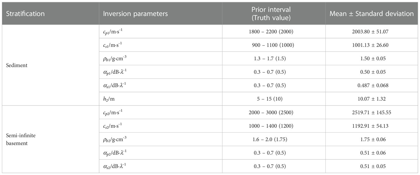
Table 1 Inversion results of seabed parameters in the simulation environment.

$\begin{array}{ll}\{\begin{array}{c}\text{T}{\text{L}}_p=-201\text{g}\left|\frac{p(r,z,\omega }{p_{ref}{|}_{r-1m}}\right|p_{ref}=\frac{{\text{e}}^{i{k}_{0}r}}{r}\\ \text{T}{\text{L}}_{v_z}=-201\text{g}\left|\frac{v_z(r,z,\omega }{v_{ref}{|}_{r-1m}}\right|v_{ref}=\frac{k_0}{\rho \omega }\frac{{\text{e}}^{i{k}_{0}r}}{r}\\ Z{L}_{z_z}=10\lg \left|\frac{Z_z(r,z,\omega )}{Z_{ref}}\right|Z_{ref}=1.48\times {10}^6\text{Pa}·\text{s}/\text{m}\end{array}& (22)\end{array}$

Figures 2A–C show the propagation characteristic curves in Table 1 for the p, v_z and Z_z, respectively. The transmission loss curves TL_p and TL_vz are used to describe the propagation characteristic of p and v_z, and the waveguide characteristic impedance curve ZL_Zz is used to describe the propagation characteristic of Z_z. These curves are defined by Equation (22) (Zhu, 2014).

FIGURE 2

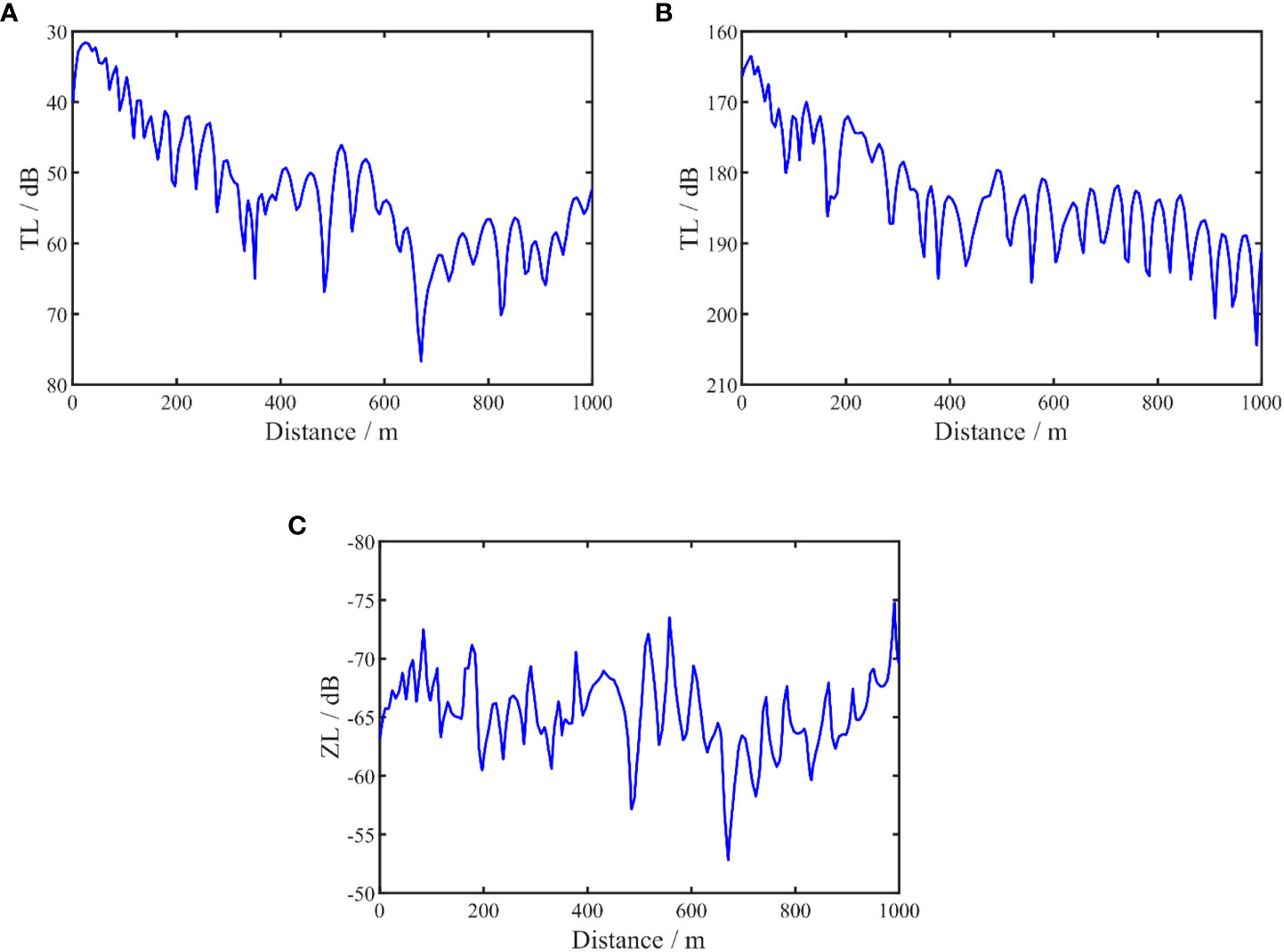
Figure 2 The calculated level for the p, v_z and Z_z, respectively. acoustic pressure (A), vertical particle velocity (B) and waveguide characteristic impedance (C).

From the comparison results, it can be seen that at some distances, that lead to notable peaks of the waveguide characteristic impedance Z_z, these peaks contain important information from the environment. This fluctuation is evident at short distances. As the propagation distance increases, the numerical value decreases at long distances decreases, and the change is relatively weakened. The fluctuation of the vertical waveguide characteristic impedance is more evident in the propagation distance because its definition cancels the influence of the source level and wave front expansion. The waveguide characteristic impedance also compensates for the transmission loss caused by the expansion of the wavefront, which is more conducive to the use of the waveguide information. Therefore, it is more suitable for the inversion of geoacoustic parameters as the match object.

The accuracy of the inversion result strongly depends on the sensitivity of the physical quantity to the geoacoustic parameters. The inversion results obtained with geoacoustic parameters with low sensitivity had larger uncertainty and lower inversion accuracy. When the sensitivity of a specific geoacoustic parameter is discussed in the inversion, the other parameters are fixed and only change the value of the discussed parameter within the range of interest. The value of the error function E(m) for the discussed parameter reflects its sensitivity within the range of interest.

The sensitivities of p, v_z, and Z_z to the geoacoustic parameters in Table 1 are compared in Figures 3, 4. The two figures show the comparative results for the geoacoustic parameters in sediment and basement for a frequency of 150 Hz. In these figures, the blue curve represents p, the black curve represents v_z, and the red curve represents Z_z. The results show that Z_z is much more sensitive to these geoacoustic parameters than p or v_z, all the parameters will have an impact on the E(m) for Z_z. Z_z shows higher sensitivity to wave speed and sediment layer thickness than to density and sound speed attenuation. The sensitivities of p and v_z were relatively close in the sediment and basement layers. Among the other parameters, the sensitivity of sound speed attenuation is relatively low, but Z_z has the most significant improvement in the sensitivity of these parameters. This means that using Z_z as the match object can improve the accuracy of the inversion results, especially for the sound speed attenuation.

FIGURE 3

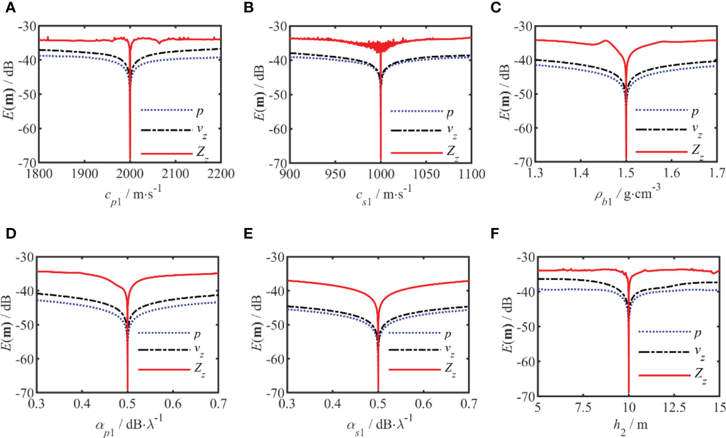
Figure 3 The sensitivity analysis of the error function E(m)) for the geoacoustic parameters of the sedimentary layers. (A–F) corresponds to the c_p1, c_s1, ρ_b1, α_p1, α_s1, and h₂, respectively. The red curve represents is for the vertical waveguide characteristic impedance, and the black curve represents the vertical particle velocity and blue curve is for the acoustic pressure.

FIGURE 4

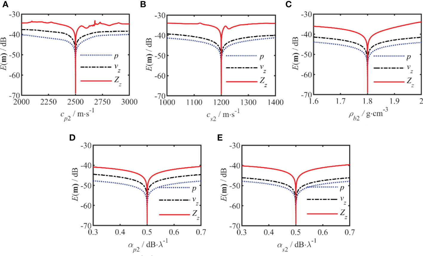
Figure 4 The sensitivity analysis of the error function E(m)) for the geoacoustic parameters of the semi-infinite seabed. (A–E) corresponds to the c_p2, c_s2, ρ_b2, α_p2, and α_s2, respectively. The red curve represents for the vertical waveguide characteristic impedance, the black curve represents the vertical particle velocity and blue curve is for the acoustic pressure.

According to the above analysis results, Z_z has been shown to have higher sensitivity to geoacoustic parameters than p and v_z. Z_z is expected to provide higher precision for geoacoustic parameters in geoacoustic inversion than when only p or v_z is used, especially for sound speed attenuations.

4.2. Simulation inversion results

In this section, the feasibility of the Bayesian inversion method using the characteristic impedance of a vertical waveguide is studied through simulations. In the simulation, the shallow sea model, listed in Table 1, was selected as the measurement environment. The true values of the geoacoustic parameters for the two-layered structure of the seabed are the inverse objects, and the vertical waveguide characteristic impedance data, as calculated in Figure 2C, are used as the measurement data ${\text{Zz}}_{{\text{f}}_{\text{mea}}}^{}$ for matching in the inversion. The parametric search optimization is performed by minimizing Equation (21) using the adjusted optimization annealing algorithm.

Model selection was performed by evaluating different layered models using BIC to determine the simplest parameterization that matches the measured data, and the results are shown in Figure 5. The BIC values of the three inversion models with different hierarchical structures are 36.52, 34.24, and 36.93, respectively. Based on the BIC, the 2-layer model was selected as the best-parameterized model, and the selected result agreed with the specification in Table 1.

FIGURE 5

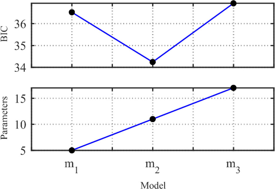
Figure 5 The result of model selection, the number of model parameters and the BIC value.

Table 1 also shows the average and standard deviation of the maximum a posteriori probability estimate of the vertical waveguide characteristic impedance inversion results. Compared with the preset true value, it can be seen that the maximum error is within 0.3%. To further verify the accuracy of the inversion results, Figure 6 shows a comparison of the waveguide characteristic impedance curve ZL_Zz calculated using the true simulation value and inversion results. From the comparison of the results in Figure 6, it can be seen that the two curves are in agreement. The root mean square (RMS) of the inversion results was 0.38 dB, which proves the reliability of the results obtained with this inversion method.

FIGURE 6

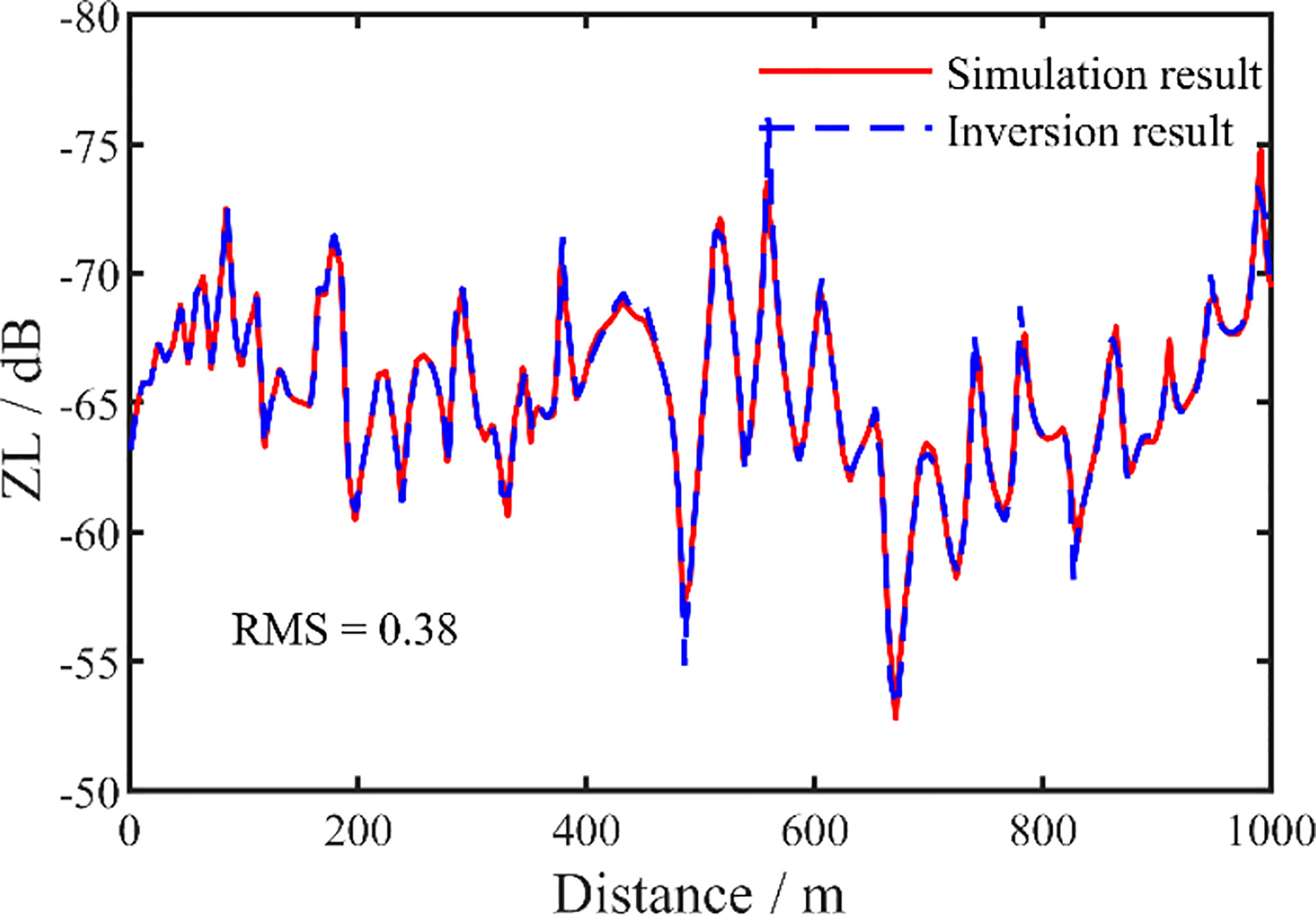
Figure 6 Comparison of the vertical waveguide characteristic impedance inversion results of simulation data. The inversion result is the dashed line and the experimental data is the solid line.

Figures 7, 8 show the PPDs of the inverted geoacoustic parameters in the sediment layer and semi-infinite basement, respectively. In each figure, the vertical axis represents the probability of each parameter and the red line represents the true simulation value of each parameter. The average value and standard deviation of the inversion results are represented by the blue segment, with the average value shown in the center. The length of the blue segment reflects the standard deviation of each parameter. The PPD distribution range characterizes the uncertainty of each parameter. It can be seen from the results that the maximum probability density of each parameter is close to its true value. The uncertainty of the inversion results for each parameter is consistent with the results of the sensitivity analysis.

FIGURE 7

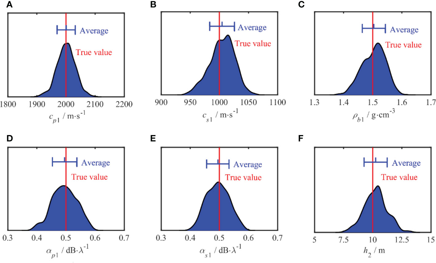
Figure 7 One-dimensional marginal probability distribution of sedimentary parameters. The red line means the true values of each parameter in simulation. The blue segments represent the average value and the standard deviation.

FIGURE 8

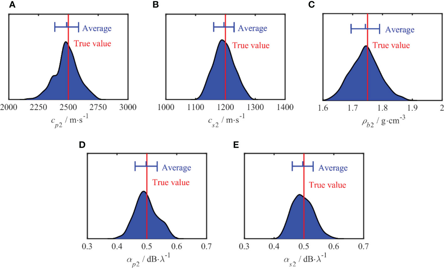
Figure 8 One-dimensional marginal probability distribution of semi-infinite parameters. The red line represents the true values of each parameter in the simulation. The blue segments represent the average value and the standard deviation.

The marginal probability distribution between the two parameters is shown in Figure 9, which shows the uncertainty of the joint parameters. From the figures, it can be seen that the centralized probability density distributions characterize lower uncertainties, and all true values are close to the highest probability of PPD. The results combined with the sound speed attenuation have a broader distribution, the results combined with α_s2 and α_p2 are more distinct, and the span in the attenuation direction is larger. In conjunction with the analysis of the inversion accuracy of each parameter, it can be seen that, the sound speed attenuation has little effect on the theoretical acoustic pressure field in the process of matching inversion. Therefore, many results that deviate from the true value are retained, resulting in a more comprehensive distribution range.

FIGURE 9

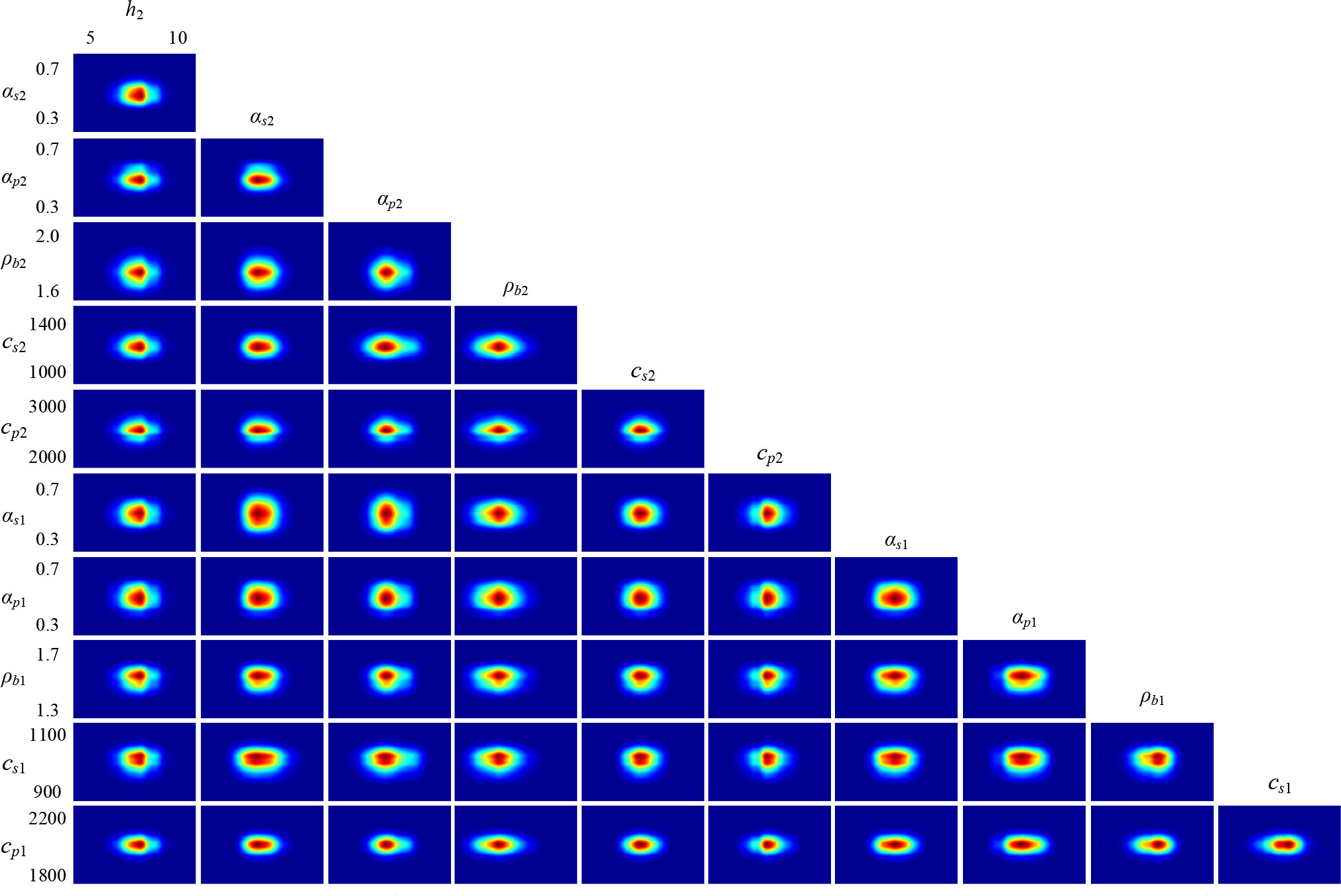
Figure 9 Two-dimensional joint marginal probability density distribution for 2-layer model.

5. Experiment results

5.1. Experiment description

To further illustrate the feasibility of the inversion method in practice, experimental data were processed and discussed. An experiment to measure sound-propagation was conducted in a shallow sea near Dalian. The water depth in the experimental area was approximately 25 m. According to previous information, the upper layer of the seabed in this sea area is sandy sediment and the lower layer is bedrock (Ren et al., 2018). During the measurement, a wideband signal was generated by the source ship engine along tracks at distance intervals of approximately 3 km, the depth of the sound source is equivalent to 1 m underwater. The signals were received by a vector hydrophone composed of acoustic pressure and vertical particle velocity in three directions, with a sampling frequency of 8192 Hz, and it is placed 5 m underwater by the receiver ship. The experimental configuration is shown in Figure 10. The deployment of the source and receiver ships are shown in Figure 10A. The motion trajectories of the two ships are shown in Figure 10B, where the solid black line represents the motion trajectory of the source ship and the solid red line represents the floating trajectory of the receiver ship during the experiment. The squares represent the recorded positions of the two ships at the beginning of the experiment and the circles represent the relative positions of the two ships at the end of the ship noise measurement. The motion trajectory of the yellow diamond represents the ambient noise measured after the experiment.

FIGURE 10

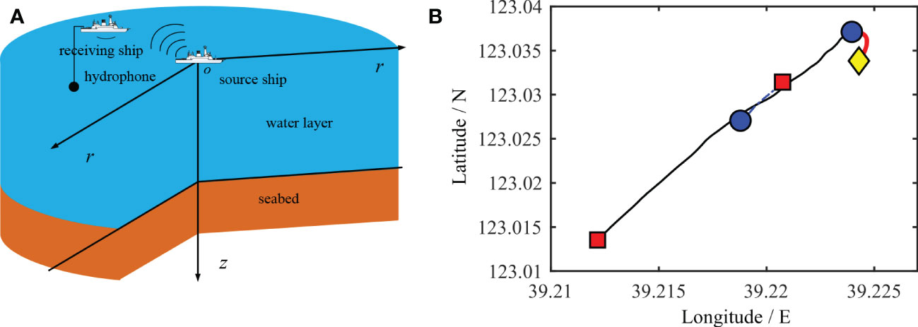
Figure 10 Schematic diagram of the experimental configuration, the deployment of the source ship and receiving ship (A) and the longitude and latitude of the distance between the two ships (B).

Before the start of the experiment, the line connecting the two ships was the x-coordinate, and the positive direction of the receiving ship was the y-coordinate. In this coordinate system, Figure 11A shows the distance between the source ship and receiving ship with time during the experiment. Figure 11B shows the relationship between the sound speed profile and the sea depth in the experimental area.

FIGURE 11

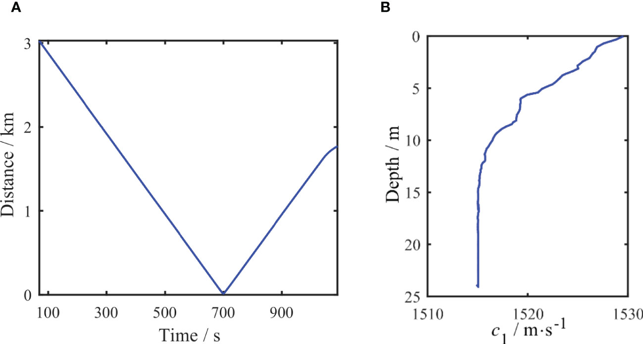
Figure 11 The distance between the source ship and the receiving ship with time during the experiment (A), and the sound speed profile of the experiment sea area (B).

Figure 12 shows the acoustic pressure signal and the vertical particle velocity signal received from the vector hydrophone in the experiment. The recorded signals in the time domain and the corresponding low-frequency analysis recording (LOFAR) images are all given. Because the distance between the source ship and the receiving ship could satisfy the “distant-near-distant” relationship during the measurement, the amplitude of the two received signals in the time domain has the characteristic of “small-large-small.” According to the LOFAR images corresponding to the signal received from each channel, the two received signals all show distinct interference striations in the range (time)–frequency domain.

FIGURE 12

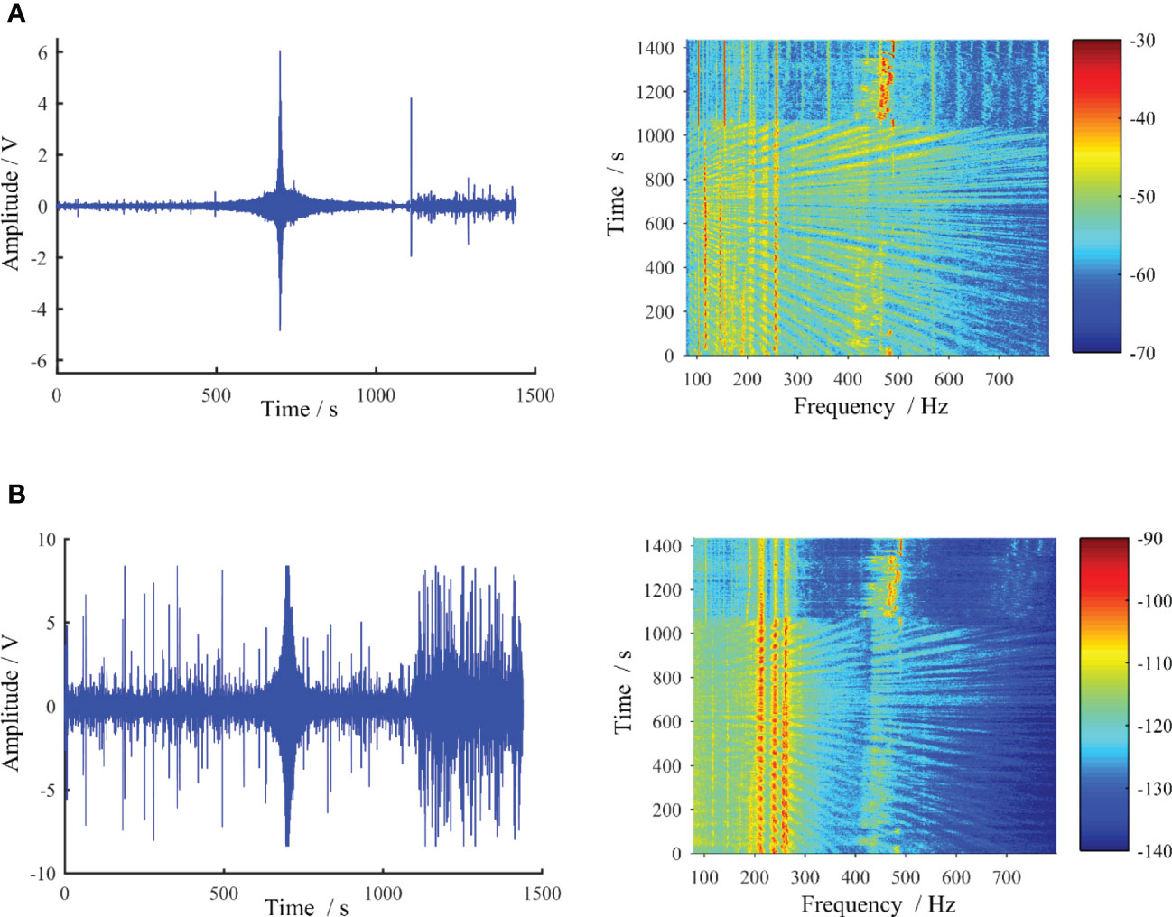
Figure 12 The recorded vector signals in time-domain and the corresponding LOFAR images, acoustic pressure (A) and vertical particle velocity (B).

To satisfy the propagation conditions of the point sources, the experimental data in the 0-700 s time period were selected for inversion. From the pressure p and the vertical particle velocity v_z measured by the vector hydrophone, the vertical waveguide characteristics impedance Z_z can be determined. To analyze the measurement results, we chose the 210 Hz signal, which can be seen more clearly in the time-frequency diagram, as the match object for the inversion. The depth of the source z_s was equal to 1 m, the depth of the vector sensor z_r=5 m, and the water depth of the experimental sea area was 25 m.

5.2. Inversion results and analysis

Model selection studies were performed for the three modes to determine the optimal parameterization for each parameter in each case. The unknown sound speed and density are assumed to depend on depth, as the acoustic pressure is mainly sensitive to these parameters. Therefore, each additional layer increases the number of parameters by six. Nonlinear optimizations for the impedance level inversion were performed to estimate the error function and hence the BIC for three different parameterizations with one to three uniform layers (including the basement layer). The results of the model selection are summarized in Figure 13 in terms of BIC values and number of layers. Note that, for intuitive presentation, the BIC values are normalized so that the minimum is unity. The results show that the lowest BIC value corresponds to the 2-layer inversion model. The inversion results (average + standard deviation) obtained with the 2-layer model are listed in Table 2, including the average and standard deviation with a confidence level of 70%. When comparing the inversion results of the same data (Ren, 2013), it was found that the speed and density of the sound were consistent within the error range.

FIGURE 13

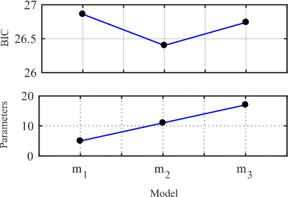
Figure 13 The result of model selection, the number of model parameters and the BIC value.

TABLE 2

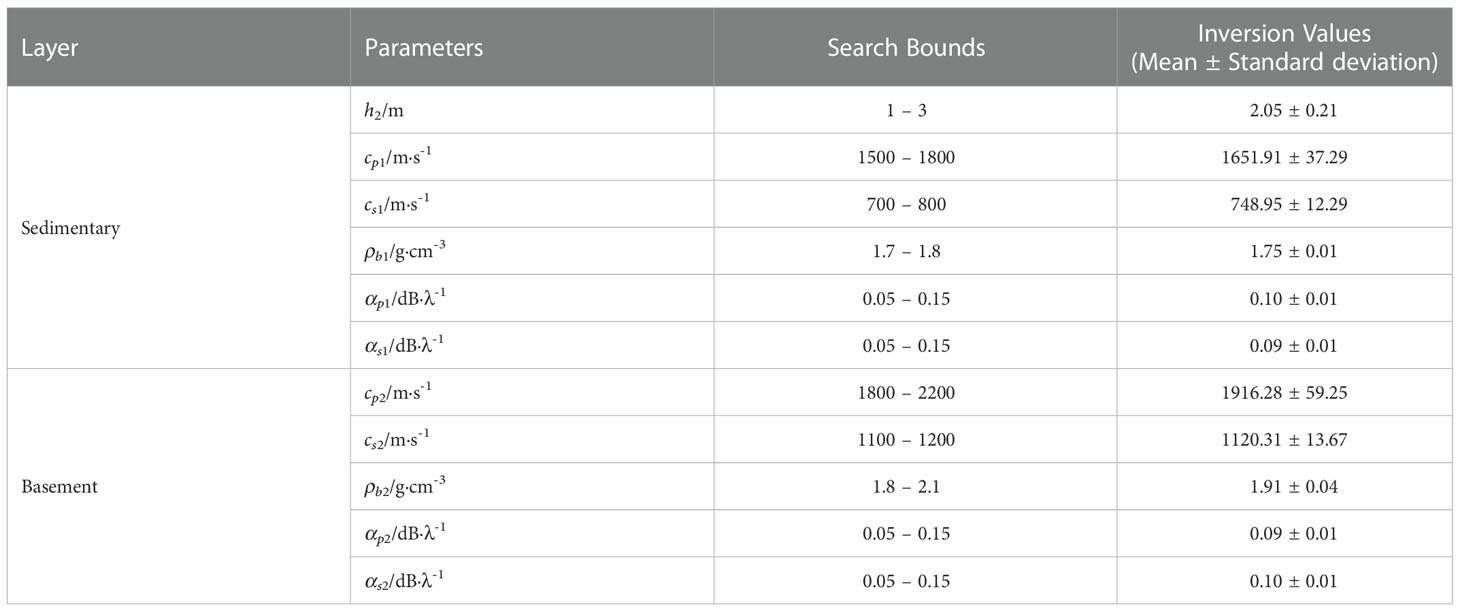
Table 2 Results of the measured data inversion.

The feasibility of the inversion method was further verified by comparing the inversion and measurement results. Figure 14 shows the comparison of the transmission loss curves TL_p (in Figure 14A) and the waveguide characteristic impedance curve ZL_Zz (in Figure 14B) obtained by the inversion of the two-layer model with the experimental data. The result of the inversion is the dashed line, and the experimental data is the solid line. Comparing the distribution trends of TL_p and ZL_Zz, it can be seen that ZL_Zz has a higher degree of consistency, especially at a larger distance. The ZL_Zz comparison results were better and showed higher stability. The RMS values of TL_p and ZL_Zz are 3.7 dB and 2.3 dB, respectively. A better fit for ZL_Zz was also indicated by the RMS values.

FIGURE 14

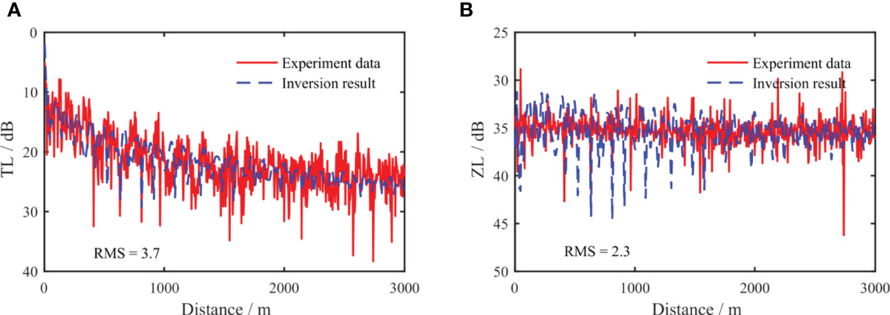
Figure 14 Comparison of inversion results of measured data. Acoustic pressure (A), vertical waveguide characteristic impedance level (B). The inversion result is the dashed line and Ex-periment data is the solid line.

The marginal probability distributions for the parameters of the two-layer model inversion are estimated using Metropolis–Hastings sampling and are shown in Figures 15, 16, respectively. The red line represents the position with the highest probability density, i.e., the MAP value, and the blue line represents the average and standard deviation of the inversion results, with the average shown in the middle of the segment. Compared to the PPDs of the simulation inversion results, the distribution range of the PPDs obtained from the experimental data is more comprehensive, indicating that they are subject to larger uncertainties, and the uncertainties of the different parameters also vary. Compared to other parameters, the parameter h₂ has a narrow peak in the sediment layer, and the distribution of the sound speed attenuation (α_p1, α_s1) in the interval is relatively flat. The uncertainty of the parameters of the semi-infinite seabed was higher than that of the sedimentary layers.

FIGURE 15

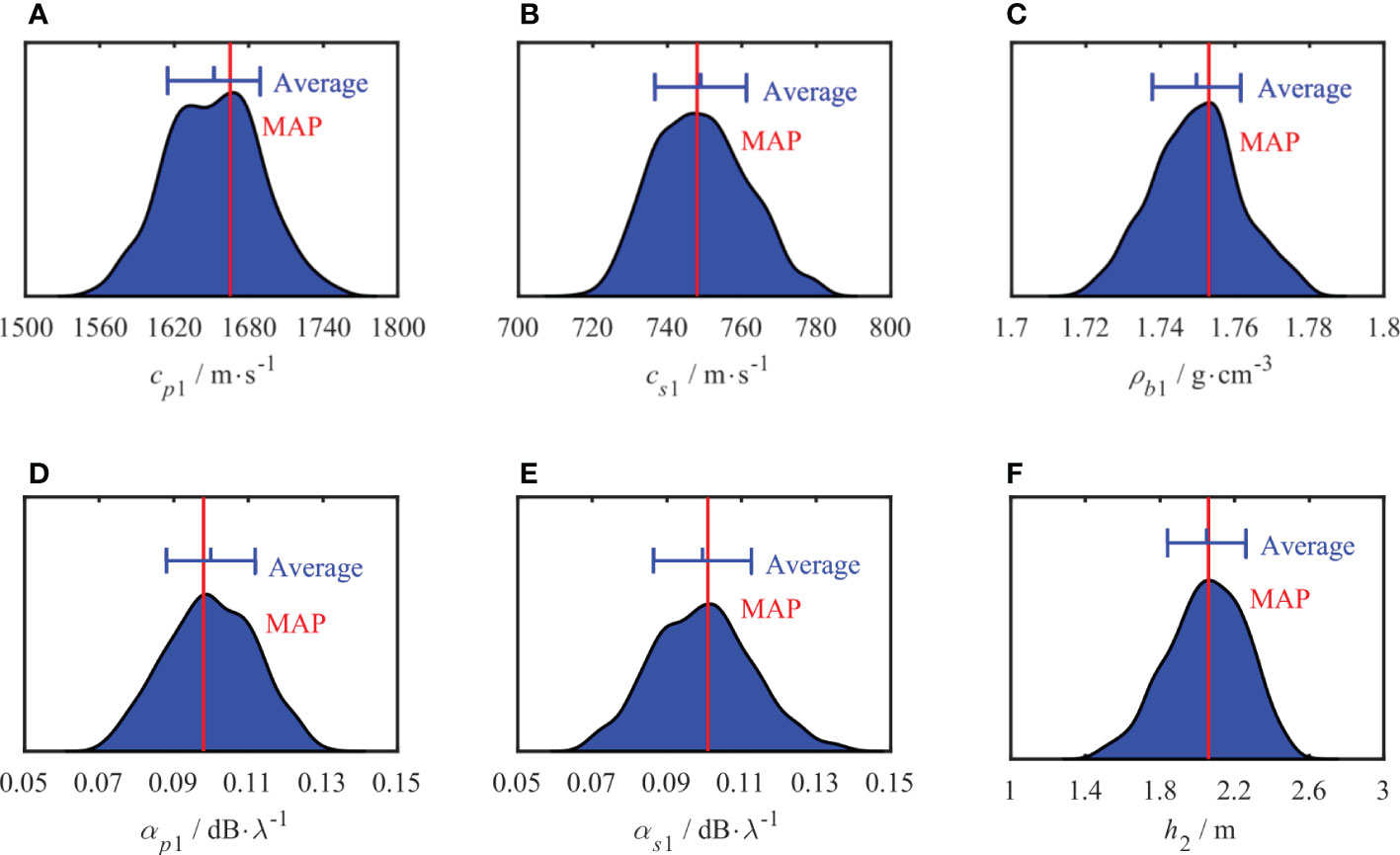
Figure 15 One-dimensional marginal probability distribution of sedimentary parameters. MAP value (red line), Average (blue vertical line in the middle) and standard deviation (blue vertical lines at both ends).

FIGURE 16

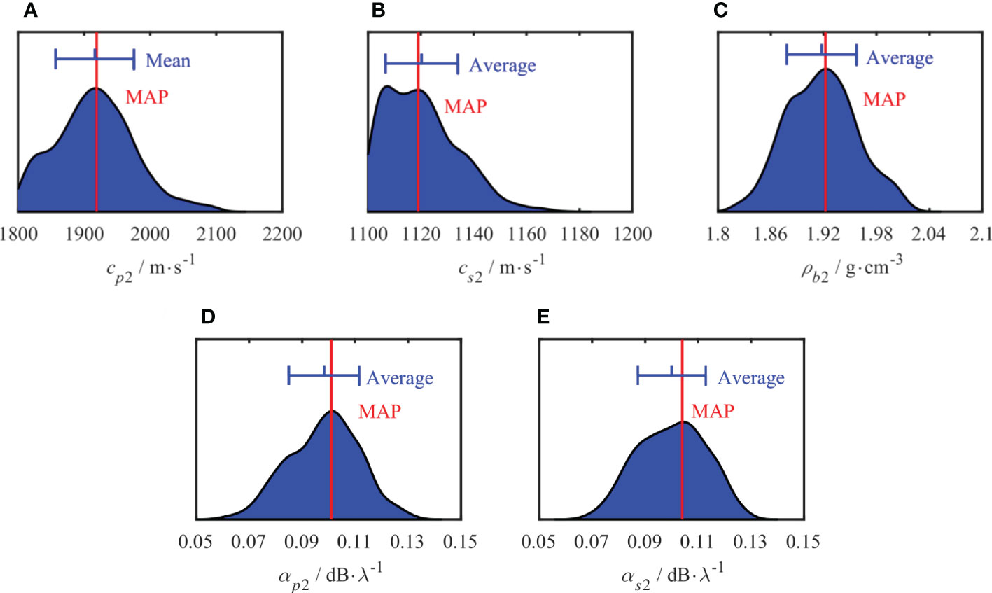
Figure 16 One-dimensional marginal probability distribution of semi-infinite parameters. MAP value (red line), Average (blue vertical line in the middle) and standard deviation (blue vertical lines at both ends).

The marginal probability distribution between the two parameters in the experimental data inversion is shown in Figure 17, which shows the uncertainty of the joint parameter. Compared with the two-dimensional probability density distribution in the simulation analysis, the distribution range obtained from the experimental data is more comprehensive, indicating that it has a higher uncertainty. This may be owing to the larger interference in the experiment. During the inversion process, more interference values affect the inversion results. This is consistent with the results of the one-dimensional probability density distribution. The probability density distribution of the individual joint parameters still exhibited a relatively obvious bright spot distribution, as shown in Figure 17. The parameters combined with h₂ are self-explanatory and have a narrower distribution range, indicating that the uncertainty of combining the two is small. With increasing depth, the fate of each parameter increased in the lower seabed compared to that in the upper layer. This feature is observed in the marginal probability distribution, and the inversion of the measured data is more evident.

FIGURE 17

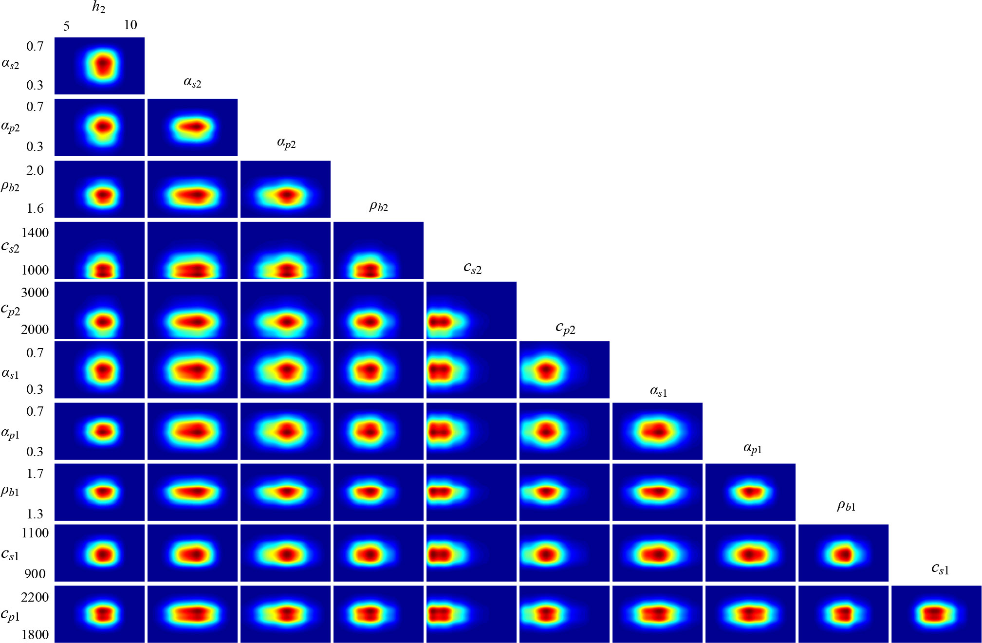
Figure 17 Two-dimensional marginal probability density distribution.

6. Conclusions

To obtain more accurate inversion results for geoacoustic parameters in shallow seas, a new geocaoustic inversion method is presented in this study based on the nonlinear Bayesian approach and set the vertical waveguide characteristic impedance Z_z as the match object,. The main conclusions are as follows:

(1) According to analysis results, in shallow sea environment with layered elastic seabed, the vertical waveguide characteristic impedance Z_z is proved has high sensitivity for geoacoustic parameters than that for p and v_z. Geoacoustic parameters include seabed structure, sound speed, density, and sound speed attenuation in seabed layers. Z_z is expected to provide higher precision for these geoacoustic parameters in geoacoustic inversion than the single acoustic pressure p or the single vertical particle velocity v_z, especially for sound speed attenuation, and Z_z is more suitable for geoacoustic parameter inversion.

(2) The Bayesian inversion approach can characterize the inversion result by the PPD from the statistical point of view. The best-parameterized model in inversion can be accurately selected based on the BIC. The Bayesian inversion approach can also measure the uncertainty of an inversion result. Because the inversion has a certain degree of randomness, it is more reasonable to determine the inversion result from the perspective of probability.

(3) Based on the experimental data of ship-radiated noise in the Dalian offshore area, the feasibility and reliability of the proposed inversion method were verified in practice. The sea experiment’s inversion shows that the layered structure of the seabed and geoacoustic parameters can be accurately determined by this method. The RMS between the vertical waveguide characteristic impedance and the measured impedance is 0.38 dB, and the inversion results accurately reflect the characteristics of the seabed in the experimental area, and the inversion seabed structure is accordance with the previous information of experiment area.

We anticipate that these research results will enrich existing applications of acoustic vector sensors, and can be used to develop an effective inversion method for geoacoustic parameters in complex shallow sea environments, as well as to develop underwater acoustic technologies for long-range detection in seawater.

Data availability statement

The raw data supporting the conclusions of this article will be made available by the authors, without undue reservation.

Author contributions

HZ and YX processed data, and co-authored wrote the original manuscript. QR supervised the study and reviewed the manuscript. XL and JW contributed to image format modification. ZC contributed to data. SZ and HF reviewed the manuscript. All authors contributed to the article and approved the submitted version.

Funding

This research was found by the Zhejiang Province key research and development program (Grant No: 2020C02004), the Science Foundation of Donghai Laboratory (Grant No: DH-2022KF01018), the Marine defense Innovation Fund (Grant No: JJ-2020-701-09), the Science Foundation of Key Laboratory of Submarine Geosciences (Grant No: KLSG2201), Marine Science Zhejiang First-class Discipline Open Project Funding Project (Grant No: OFMS005).

Acknowledgments

We acknowledge the National Key Laboratory, College of Underwater Acoustic Engineering, Harbin Engineering University, China for supporting in this research.

Conflict of interest

The authors declare that the research was conducted in the absence of any commercial or financial relationships that could be construed as a potential conflict of interest.

Publisher’s note

All claims expressed in this article are solely those of the authors and do not necessarily represent those of their affiliated organizations, or those of the publisher, the editors and the reviewers. Any product that may be evaluated in this article, or claim that may be made by its manufacturer, is not guaranteed or endorsed by the publisher.

References

Dahl P.-H., Dall'Osto D.-R. (2020). Estimation of seabed properties and range from vector acoustic observations of underwater ship noise. J. Acoust. Soc Am. 147, 345–350. doi: 10.1121/10.0001089

CrossRef Full Text | Google Scholar

Dahl P.-H., Dall'Osto D.-R. (2022). Range-dependent inversion for seabed parameters using vector acoustic measurements of underwater ship noise. IEEE J. Ocean Eng. 47, 682–689. doi: 10.1109/JOE.2021.3086880

CrossRef Full Text | Google Scholar

Dosso S.-E., Dong H., Duffaut K. (2017). Model selection for profile structure in Bayesian geoacoustic inversion. Acoust. Soc Am.J. 14, 3470–3470. doi: 10.1121/1.4987215

CrossRef Full Text | Google Scholar

Guo X.-L., Yang K.-D., Ma Y.-L. (2017). Geoacoustic inversion for bottom parameters via Bayesian theory in deep ocean. Chin. Phys. Lett. 34, 68–72. doi: 10.1088/0256-307X/34/3/034301

CrossRef Full Text | Google Scholar

Hermand J.-P. (1999). Broad-bandgeoacoustic inversion in shallow sea from waveguide impulse response measurements on a single hydrophone: theory and experimental results. IEEE J. Ocean. Eng. 24, 41–66. doi: 10.1109/48.740155

CrossRef Full Text | Google Scholar

Huang Y.-W., Yang S.-E. (2010). Spatial-temporal coherence of acoustic pressure and particle velocity in surface-generated noise. J. Harbin. Eng. Univ. 31, 137–143. doi: 10.3969/j.issn.1006-7043.2010.02.001

CrossRef Full Text | Google Scholar

Jeon Y., Lee S.-J., Kim S. (2022). Estimation of shallow s-wave structures from the quasi-transfer spectrum and Bayesian inversion using microarray data at a deep drilling site at chungnam. Geosci. J. 26, 367–383. doi: 10.1007/s12303-021-0034-2

CrossRef Full Text | Google Scholar

Jiang X.-D., Zhang W. (2022). The research on Bayesian inference for geophysical inversion. Rev. Geophys. Planet. Phys. 53, 159–171. doi: 10.19975/j.dqyxx.2021-042

CrossRef Full Text | Google Scholar

Kavoosi V., Dehghani M.-J., Javidan R. (2021). Underwater acoustic source positioning by isotropic and vector hydrophone combination. J. Sound Vib. 501, 116031. doi: 10.1016/J.JSV.2021.116031

CrossRef Full Text | Google Scholar

Li X.-M., Piao S.-C., Zhang M.-H., Liu Y. (2019). A passive source location method in a shallow water waveguide with a single sensor based on Bayesian theory. Sensors 19, 1452. doi: 10.3390/s19061452

PubMed Abstract | CrossRef Full Text | Google Scholar

Li W.-L., Qiu J.-S., Lei P.-Y., Chen X.-H., Fan F., Deng X.-J., et al. (2022). A real-time passive acoustic monitoring system to detect Yangtze finless porpoise clicks in ganjiang river, China. Front. Mar. Sci. 9. doi: 10.3389/fmars.2022.883774

PubMed Abstract | CrossRef Full Text | Google Scholar

Li F.-H., Zhang R.-H. (2000). Bottom sound speed and attenuation inverted by using pulsed waveform and transmission loss. Acta Acustica. 25, 297–302. doi: 10.3321/j.issn:0371-0025.2000.04.002

CrossRef Full Text | Google Scholar

Miao Y.-J., Li J.-H., Sun H.-X. (2021a). Multimodal sparse time-frequency representation for underwater acoustic signals. IEEE J. Ocean. Eng. 46, 642–653. doi: 10.1109/JOE.2020.2987674

CrossRef Full Text | Google Scholar

Miao Y.-J., Zakharov V.-Z., Sun H.-X., Li J.-H., Wang J.-F. (2021b). Underwater acoustic signal classification based on sparse time-frequency representation and deep learning. IEEE J. Ocean. Eng. 46, 952–962. doi: 10.1109/JOE.2020.3039037

CrossRef Full Text | Google Scholar

Park C., Seong W., Gerstoft P. (2005). Geoacoustic inversion in time domain using ship of opportunity noise recorded on a horizontal towed array. J. Acoust. Soc Am. 117, 1933–1941. doi: 10.1121/1.1862574

PubMed Abstract | CrossRef Full Text | Google Scholar

Ren Q.-Y. (2013). Using ship noise for ocean bottom geoacoustic parameters inversion (Harbin. Eng. Univ: Harbin, China). doi: 10.7666/d.D430310

CrossRef Full Text | Google Scholar

Ren Q.-Y., Hermand J.-P. (2013). “Passive pressure and vector geoacoustic inversion offshore Amazon Rio mouth: A sensitivity study,” in Acoustics in Underwater Geosciences Symposium (RIO Acoustics) (IEEE) Rio de Janeiro, Brazil, 1–4. doi: 10.1109/rioacoustics.2013.6683979

CrossRef Full Text | Google Scholar

Ren Q.-Y., Piao S.-C., Ma L., Guo S.-M., Liao T.-J. (2018). Geoacoustic inversion using ship noise vector field. J. Harbin Eng. Uni. 39, 236–240. doi: 10.11990/jheu.201609031

CrossRef Full Text | Google Scholar

Rong S., Xu Y. (2022). Motion parameter estimation of AUV based on underwater acoustic doppler frequency measured by single hydrophone. Front. Mar. Sci. 9. doi: 10.3389/fmars.2022.1019385

PubMed Abstract | CrossRef Full Text | Google Scholar

Santos P., Rodríguez O., Felisberto P., Jesus S. (2009). “Geoacoustic matched-field inversion using a vertical vector sensor array,” in Int. Conf. Underwater. Acoust. Measurements. (UAM), Nafplion: Greece, 1–3

Google Scholar

Sun D.-J., Ma C., Yang T.-C., Mei J.-D., Shi W.-P. (2020). Improving the performance of a vector sensor line array by deconvolution. IEEE J. Ocean Eng. 45, 1063–1077. doi: 10.1109/JOE.2019.2912586

CrossRef Full Text | Google Scholar

Sun M., Li F.-H., Zhu L.-M. (2013). Geoacoustic inversion with a vector sensor array in shallow sea water. Tech. Acoust. 32, 73–74. doi: 10.1063/1.4765947

CrossRef Full Text | Google Scholar

Tollefsen D., Dosso S.-E. (2020). Ship source level estimation and uncertainty quantification in shallow water via Bayesian marginalization. J. Acoust. Soc Am. 147, 339–344. doi: 10.1121/10.0001096

CrossRef Full Text | Google Scholar

Xing C.-X., Wu Y.-W., Xie L.-X., Zhang D.-Y. (2021). A sparse dictionary learning-based denoising method for underwater acoustic sensors. Appl. Acoust. 180, 108140.1–108140.13. doi: 10.1016/j.apacoust.2021.108140

CrossRef Full Text | Google Scholar

Yang H., Lee K., Choo Y., Kim K. (2020). Underwater acoustic research trends with machine learning: ocean parameter inversion applications. J. Ocean. Eng. Technol. 34, 371–376. doi: 10.26748/KSOE.2020.016

CrossRef Full Text | Google Scholar

Yu S.-W., Xiao L., Sun W.-T. (2022). Parameter measurement of aircraft-radiated noise from a single acoustic sensor node in three-dimensional space. Front. Mar. Sci. 9. doi: 10.3389/fmars.2022.996493

PubMed Abstract | CrossRef Full Text | Google Scholar

Zhang X.-B., Wu H.-R., Sun H.-X., Ying W.-W. (2021). Multireceiver SAS imagery based on monostatic conversion. IEEE J-STARS 14, 10835–10853. doi: 10.1109/JSTARS.2021.3121405

CrossRef Full Text | Google Scholar

Zhang X.-B., Yang P.-X., Dai X.-T. (2019). Focusing the multireceiver SAS data based on the fourth order Legendre expansion. Circ. Syst. Signal Pr. 38, 2607–2629. doi: 10.1007/s00034-018-0982-6

CrossRef Full Text | Google Scholar

Zhang X.-B., Yang P.-X., Huang P., Sun H.-X., Ying W.-W. (2022). Wide-bandwidth signal-based multireceiver SAS imagery using extended chirp scaling algorithm. IET Radar Sonar Nav. 16, 531–541. doi: 10.1049/rsn2.12200

CrossRef Full Text | Google Scholar

Zhang H.-G., Yang S.-E., Piao S.-C., Ren Q.-Y., Ma S.-Q. (2010). A method for calculating an acoustic vector field. J. Harbin. Eng. Univ. 31, 470–475. doi: 10.3969/j.issn.1006-7043.2010.04.011

CrossRef Full Text | Google Scholar

Zhang X.-B., Ying W.-W., Yang P.-X., Sun M. (2020). Parameter estimation of underwater impulsive noise with the class b model. IET Radar Sonar Nav. 14, 1055–1060. doi: 10.1049/iet-rsn.2019.0477

CrossRef Full Text | Google Scholar

Zhao Y.-P., Xie S.-D., Ma C. (2022). Experimental investigations on the hydrodynamics of a multi-body floating aquaculture platform exposed to sloping seabed environment. Front. Mar. Sci. 9. doi: 10.3389/fmars.2022.1049769

PubMed Abstract | CrossRef Full Text | Google Scholar

Zheng G.-X., Piao S.-C., Zhu H.-H., Zhang H.-Z., Li N.-S. (2021). Bayesian Inversion method of geoacoustic parameter in shallow sea using acoustic pressure field. J. Harbin. Eng. Univ. 42, 497–504. doi: 10.11990/jheu.201906062

CrossRef Full Text | Google Scholar

Zheng G.-X., Zhu H.-H., Wang X.-H., Sartaj K., Li N.-S., Xue Y.-Y. (2020). Bayesian Inversion for geoacoustic parameters in shallow Sea. Sensors 20, 2150. doi: 10.3390/s20072150

PubMed Abstract | CrossRef Full Text | Google Scholar

Zhou J.-B., Tang J., Yang Y.-X. (2021). A study on the estimation of source bearing in an ASA wedge: Diminishing the estimation error caused by horizontal refraction. J. Mar. Sci. Eng. 9, 1449. doi: 10.3390/jmse9121449

CrossRef Full Text | Google Scholar

Zhu H.-H. (2014). Geoacoustic parameters inversion based on vertical waveguide characteristic impedance in acoustic vector field (Harbin. Eng. Univ: Harbin, China). doi: 10.7666/d.D749708

CrossRef Full Text | Google Scholar

Zhu H.-H., Piao S.-C., Zheng H., Zhang H.-G., Tang Y.-F. (2015). Research on geoacoustic parameters inversion in shallow sea from acoustic impedance. Tech. Acoust. 34, 204–206.

Google Scholar

Zhu H.-H., Zhu J., Tang J., Zhang H.-G., Zheng G.-X. (2020). Effect of sediment acoustic characteristics on low-frequency acoustic field distribution in shallow water. Acta Acustica 45, 664–674. doi: 10.15949/j.cnki.0371-0025.2020.05.006

CrossRef Full Text | Google Scholar