Biomass prediction method of nuclear power cold source disaster based on deep learning

Given the insufficient early warning capacity of nuclear cold source biological disasters, this paper explores prediction methods for biomass caused by nuclear cold source disasters based on deep learning. This paper also uses the correlation analysis method to determine the main environmental factors. The adaptive particle swarm optimization method was used to optimize the depth confidence network model of the Gaussian continuous constrained Boltzmann machine (APSO-CRBM-DBN). To train the model, the marine environmental factors were used as the main input factors and the biomass after a period of time was used as the output for training. Optimal prediction results were obtained, and thus, the prediction model of biomass caused by the nuclear cold source disaster was established. The model provides an accurate scientific basis for the early warning of cold source disasters in nuclear power plants and has important practical significance for solving the problem of biological blockage at the inlet of cold source water in nuclear power plants.

1 Introduction

In recent years, with the change of marine ecological environment, the water inlet blockage of nuclear power source caused by marine organisms has become more and more serious (Tang et al., 2017). The nuclear safety accident and economic loss caused by it have been paid more and more attention by all countries in the world. Since 2004, there have been nearly 200 clogged intakes at nuclear power plants around the world, the vast majority of which are caused by jellyfish, seaweed, aquatic plants, shellfish, fish, and other marine organisms. These blockages lead to power reduction or reactor shutdown of units, which seriously affects the safe operation of nuclear power plants (Ruan, 2015; Tang et al., 2017). In the winter of 2014 and 2015, the phaeocystis red tide in the coastal waters of Guangxi covered the waters near Fangchenggang, and the phaeocystis (2–3 cm) clogged the filter apparatus, posing a threat to the safety of the cold source system of nuclear power facilities. In December 2009, a large number of water weeds invaded and blocked the filtration system of the pump station of unit 4 of the CRUAS nuclear power plant in France, resulting in the loss of cold source of the unit (Tang et al., 2017). In 2012, a large number of jellyfish invaded the cooling water system of a nuclear power plant in California, USA (Tang et al., 2017). In July 2014, a large number of jellyfish flooded into the intake of the circulating water filtration system of the Hongyanhe Nuclear Power Plant, leading to the shutdown of Unit H1/2. In August 2015, a large number of Haitian melons rushed into the water inlet of Ningde No. 3 unit, resulting in unit shutdown operation. In January 2016, the No. 2 unit of the Lingao Nuclear Power Plant was in emergency shutdown due to the influx of shrimp into the water intake (Meng et al., 2018; Meng et al., 2019; Zhang et al., 2020). In April 2018, just at the critical time of the Boao Forum for Asia, a large amount of seaweed flooded into the Changjiang Nuclear Power Plant in Hainan Province, blocking the drum filter screen and causing the circulating water pump to trip. Two units of the Changjiang Nuclear Power Plant were shut down, and the whole plant lost power supply to the outside world. Marine biological disaster is an urgent problem facing the safety of our coastal nuclear power operation.

In order to prevent or reduce the impact of marine disaster-causing organisms, domestic and foreign nuclear power plants have also taken active defense measures. The main approach is to develop a marine disaster biological monitoring system, in order to give early warning before the disaster-causing organisms reach the grid and filter drum network. Kim and Myung (2018); Kim et al. (2016) collected jellyfish videos on the water surface with cameras mounted on drones, identified and calculated the density of jellyfish in the video frame images, monitored the biomass of disaster-causing organisms in real time, and made track prediction in combination with meteorological and hydrodynamic environment, which could play an early warning role to a certain extent and gain the response time to take measures such as fishing and interception. Meng et al. (2018) established underwater acoustic detection and optical imager for real-time monitoring of marine organisms in the waters near the nuclear power intake. When the biomass reaches a certain threshold, the system software starts to give an early warning. Martin-Abadal et al. (2020) proposed a jellyfish real-time monitoring system based on the deep learning method. The deep learning model processes underwater monitoring videos to realize jellyfish identification and quantitative estimation. A number of scholars (Yang et al., 2018; French et al., 2019; Han et al., 2022) have developed a real-time monitoring system of underwater sonar image, which, combined with hydrodynamic elements, and based on algorithms such as neural networks, gives early warning to marine organisms. However, in many cases, the accumulation rate of disaster-causing organisms is very fast. When the biomass is detected to increase sharply, the response time left for nuclear power plants is very short. Therefore, relying only on real-time monitoring system cannot fundamentally solve the problem. The most effective approach is to develop an early warning system for marine catastrophes to realize early warning before the catastrophes arrive at the grid and filter drum network. At this time, the establishment of an accurate biomass prediction model is an important scientific basis for the system to realize early warning.

A highly nonlinear model between marine environmental parameters and disaster-induced biomass is needed to predict the biomass of nuclear cold sources. Highly nonlinear models are usually constructed by training on traditional artificial neural networks or machine learning methods, such as deep learning. Many biological prediction models for red tide algal blooms have been built by scholars from various countries based on marine environmental data (Zohdi and Abbaspour, 2019), but few prediction models for organisms are caused by nuclear cold sources. Based on the analysis of marine environmental data, this paper uses the mixed APSO-CRBM-DBN deep learning algorithm to study a prediction method that can accurately predict disaster-induced biomass of nuclear power cold sources. We have built an accurate prediction model for the disaster-induced biomass of nuclear power cold sources.

2 Methodology

In this paper, the correlation analysis of marine environmental monitoring data and disaster-causing biomass data was carried out by using the multi-factor correlation analysis method, and the main influencing parameters were determined. Nuclear disaster-causing organisms are affected by a variety of marine environmental factors, and the mapping relationship is nonlinear; thus, it is difficult to predict using the regression model. Therefore, this paper builds a deep confidence network model, trains marine environmental data and pointed pen cap data, and obtains a prediction model suitable for predicting the disaster-causing biomass of nuclear cold source.

2.1 Model input influence factor determination

Organisms that cause nuclear disasters are comprehensively affected by marine environmental parameters. These environmental impact parameters vary for different organisms. Therefore, to improve the accuracy of the model, it is necessary to more accurately determine the environmental parameters affecting the proliferation and aggregation of relevant organisms. In this study, the input environmental impact parameters were selected as comprehensively as possible. The autocorrelation coefficient method was then used to calculate the contribution of each parameter to the biomass, and the correlation coefficients between the parameters were used to calculate the correlation between the parameters. The range of environmental parameters was refined as well.

The correlation coefficient between parameters denotes the covariance of the multivariate parameter matrix. In multivariate probability statistics, the spread matrix is a statistic used to estimate the covariance of a multidimensional normal distribution. An n-dimensional sample represents the adoption of n different environmental parameters, where each dimension represents the time series of one parameter. The matrix X of m x n represents the data matrix of the above n parameters, where X=[x₁,x₂, ,x_n]. The sample mean is $\overline{x}=\frac{1}{n}{\displaystyle \sum _{j=1}^n{x}_j}$, where x_j is the jth column in X. The semi-positive definite matrix of the dispersion matrix is as follows:

$\begin{array}{ll}\begin{array}{c}S={\displaystyle \sum _{j=1}^n\left(x_j-\overline{x}\right)}{\left(x_j-\overline{x}\right)}^T\\ =\left({\displaystyle \sum _{j=1}^n{x}_j{x}_j^T}\right)-nx{\overline{x}}^T\end{array}& (1)\end{array}$

In the formula, the dispersion matrix S=XC_nX^TC_nX^T, where C_n is the centering matrix. The equation to calculate C_n is as follows:

$\begin{array}{ll}{C}_n=I_n-\frac{1}{n}O& (2)\end{array}$

where O represents the matrix with all the elements equal to 1. In maximum likelihood estimation, given n data samples, the covariance C_ML of a multidimensional normal distribution can be expressed as a normalized divergence matrix, and the correlation coefficient between multiple parameters can be obtained.

$\begin{array}{ll}{C}_{ML}=\frac{1}{n}S& (3)\end{array}$

In this paper, the autocorrelation coefficient method was adopted to calculate the contribution of environmental parameters to biomass. The time series of biomass and other environmental parameters is defined as X and Y, and the number of elements is N (N represents the length of the time series), where x_i and y_i are elements in X and Y, respectively, and $\overline{x}$,$\overline{y}$ are sample means, respectively. The correlation coefficient is defined mathematically as:

$\begin{array}{ll}r=\frac{{\displaystyle \sum _{i=1}^n\left(x_i-\overline{x}\right)\left(y_i-\overline{y}\right)}}{\sqrt{{\displaystyle \sum _{i=1}^n{\left(x_i-\overline{x}\right)}^2{\displaystyle \sum _{i=1}^n{\left(y_i-\overline{y}\right)}^2}}}}& (4)\end{array}$

2.2 Model design

The model consists of a visible layer, a hidden layer, and an output layer. The input layer is continuously monitoring data, including ecological, hydrodynamic, and other environmental parameters and biomass. The input layer data are represented by x(t),t=1,2, ,T, where T is the number of samples in the data time series. the output layer is the biomass at time t + MT, and M can be flexibly adjusted according to the specific prediction time. Figure 1 shows the biomass prediction model structure of a nuclear cold source disaster.

FIGURE 1

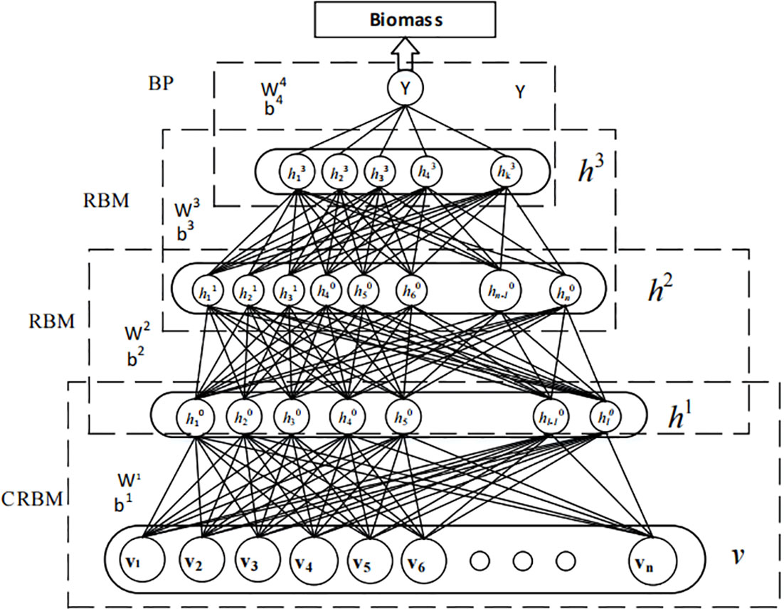
Figure 1 Biomass prediction model of nuclear cold source disaster.

If the output matrix after model learning is Y, there is the output:

$\begin{array}{ll}Y=u(X)& (5)\end{array}$

In the formula above, u(X) is the deep learning model function.

2.3 Algorithm design

The algorithm formula based on the CRBM-DBN prediction model is:

$\begin{array}{ll}\begin{array}{l}E\left(v,h;\theta \right)={\displaystyle \sum _{i=1}^n\frac{{\left(v_i-a_i\right)}^2}{2{\delta }_i^2}}-\\ {\displaystyle \sum _{j=1}^m{b}_j{h}_j}-{\displaystyle \sum _{i=1}^n{\displaystyle \sum _{j=1}^m\frac{w_{ij}{v}_i{h}_j}{{\delta }_i^2}}}\end{array}& (6)\end{array}$

In Equation (6), θ={ ω,a,b } ={ ω=(ω_ij)_n×m,a=(a_i)_n,b=(b_j)_m } is the parameter of CRBM; and are the vectors of visible and hidden elements of CRBM, respectively. ω_ij is the weight of symmetric connection between the visible cell, v_i, and the hidden cell, h_j. a₁ is the bias of the visible layer element, v_i, and b_j is the bias of the hidden element, h_j. ${\delta }_i^2$ is the standard deviation of the Gaussian noise of the visible layer element, v_i. n and m are the numbers of visible element, v_i, and the hidden element, h_j, respectively, and δ_i is the standard variance vector of the visible layer Gaussian.

There is no link in the CRBM layer of the prediction model, and the conditional probability of visible layer and hidden layer elements can be calculated by Equations (7) and (8):

$\begin{array}{ll}\begin{array}{l}P\left(h_j=1\mid v\right)=\\ \sigma \left({\displaystyle \sum _{i=1}^n{w}_{ij}{v}_i+b_j}\right)\end{array}& (7)\end{array}$

$\begin{array}{ll}P\left(v_i=1\mid h\right)=N\left({\sigma }_i{\displaystyle \sum _{j=1}^m{w}_{ij}{h}_j+a_i,{\sigma }_i^2}\right)& (8)\end{array}$

where σ(x) is the sigmoid activation function, and its expression is σ(x)=(1+e^−x)⁻¹ , N(μ,V) , which represents the Gaussian function with expectation μ and variance V. In order to characterize the complex nonlinear relationship between input and output variables, the prediction model was trained by combining unsupervised and supervised trainings.

2.4 Optimization based on the APSO algorithm

The prediction accuracy of the deep learning model depends mainly on the hyperparameters composed of the learning rate, the number of hidden layer neurons, and the number of hidden layers. However, there is no set of perfect methods to guide the selection of these parameters. This paper uses an adaptive particle swarm optimization algorithm (APSO) to improve the global search ability based on the basic particle swarm optimization algorithm (PSO). This algorithm has fast convergence speed, high precision, and better-optimized performance. Figure 2 shows the flowchart of the optimized model training. Figure 2A shows the training process of the prediction model, which calls the parameters optimized by APSO algorithm for model training. Figure 2B shows the flowchart of the optimization algorithm. The particle swarm optimization algorithm first initializes the hyperparameter according to the empirical value, converts the position into the form of network parameter, and regards the mean square error as the fitness value to calculate the fitness value of each particle in the particle swarm, and update it. If the fitness value is reduced to meet the condition of convergence, the optimal particle is outputted as the optimization hyperparameter of the deep learning model. The adaptive PSO algorithm mainly includes the following steps: Set the population size of the particle swarm as N, and set a four-dimensional vector for each particle. Here, X_i1 represents the learning rate, while X_i2, X_i3, and X_i4 represent the number of nodes in the hidden layer.

FIGURE 2

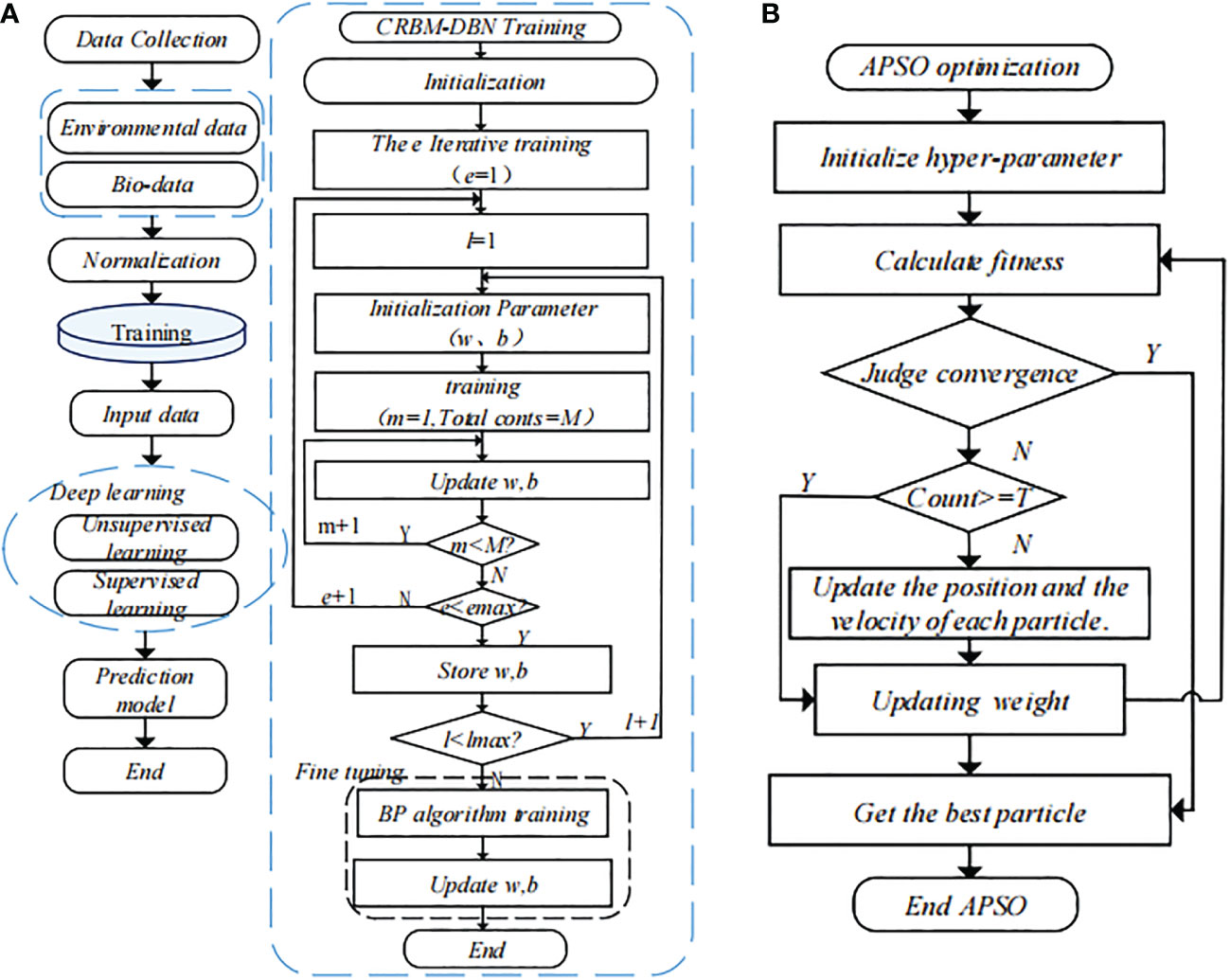
Figure 2 Training process of the APSO-CRBM-DBN disaster-induced biomass prediction model. (A) Predictive model training process. (B) APSO optimization process.

1 Read the dataset and initialize the APSO;

2 Particle 1, particle 2,… and particle n training model;

3 The reconstruction error is taken as a fitness function, and the fitness training model of each particle is calculated. The particle, $X_{pbest}^k$, with the maximum fitness and the globally optimal particle, $X_{gbest}^k$, are searched in the iteration.

$\begin{array}{ll}{F}_{fitness}=\frac{{{\displaystyle \sum _{i=1}^N{\displaystyle \sum _{j=1}^m\left(p_{ij}-t_{ij}\right)}}}^2}{N}& (9)\end{array}$

Here, N represents the number of samples in the dataset, m represents the dimension of each data, p_ij represents the reconstructed value of the j-dimension monitoring data in the ith sample in the dataset, and t_ij represents its true value.

④ The velocity and position of each particle are updated by Equations (10) and (11).

$\begin{array}{ll}\begin{array}{l}{v}_{i,t+1}^d=\omega v_{i,t}^d+c_1\ast r_1\ast \left(p_{i,t}^d-x_{i,t}^d\right)\\ +c_2\ast r_2\ast \left(p_{g,t}^d-x_{i,t}^d\right)\end{array}& (10)\end{array}$

$\begin{array}{ll}{x}_{i,t+1}^d=x_{i,t}^d+x_{i,t+1}^d& (11)\end{array}$

$\begin{array}{ll}\omega =\frac{{\omega }_{\max }-({\omega }_{\max }-{\omega }_{\max })k}{T}& (12)\end{array}$

$\begin{array}{ll}\{\begin{array}{c}{C}_1=\frac{C_{\max }-\left(C_{\max }-C_{\min }\right)k}{T}\\ C_2=\frac{C_{\max }+\left(C_{\max }-C_{\min }\right)k}{T}\end{array}& (13)\end{array}$

Above, ω , C₁, and C₂ are the inertial weight and acceleration factor values at the kth iteration.C_max and C_min are the maximum and minimum initial acceleration factor values, respectively, and T is the number of iterations

⑤ Judge whether the fitness function is small enough. If it is small enough, end the algorithm training and select the optimal particle to design the prediction model. Otherwise, go to step 2 to continue the training.

3 Experiments

3.1 Dataset

To effectively verify the accuracy of the prediction model of biomass caused by nuclear power cold source disaster, combined with the training cost of the model, 200 samples were selected as the training set and 40 samples were selected as the test set from the 2,000 continuous and synchronous environmental and biological monitoring data samples obtained from the Changjiang Station of the nuclear power plant in Hainan for 4 months. The environmental parameters in the data samples mainly included temperature, salinity, chlorophyll, dissolved oxygen, flow velocity, flow direction, and wave height. Organisms mainly include nib cap snails, prawns, and phaeocystis. The paper first selected nib cap snails with high biological abundance as research objects, and then used correlation parameter analysis to select environmental parameters closely related to the organisms. Temperature, salinity, chlorophyll, and dissolved oxygen were initially selected as the main influencing parameters and as input parameters of the deep learning model. Figure 3 shows the correlation analysis between input parameters and output biological abundance. Table 1 shows partial tip cap snail abundance and environmental data.

FIGURE 3

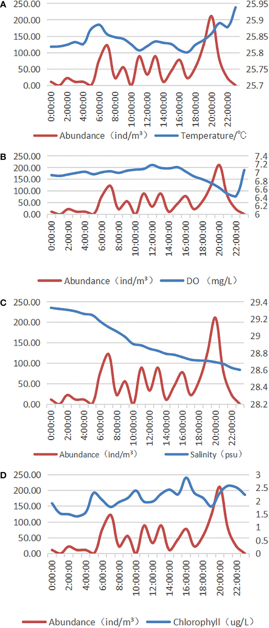
Figure 3 Input and output correlation analysis. (A) Correlation analysis between the abundance and temperature of tip pen cap snails. (B) Correlation analysis between the abundance of tip cap snails and dissolved oxygen. (C) Correlation analysis of spikelet abundance and salinity. (D) Correlation analysis between the abundance of pointy pen cap snails and chlorophyll.

TABLE 1

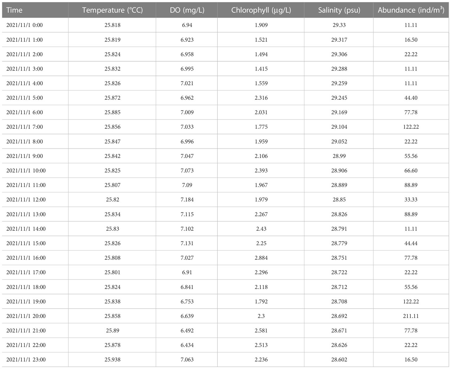
Table 1 Partial tip cap snail abundance and environmental data.

3.2 Data preprocessing

In the prediction model, temperature, salinity, chlorophyll, dissolved oxygen, and the current abundance of nib cap snails were selected as the influence factors in the input layer, and the biological abundance of nib cap snails after an interval of 24 h was selected as the output layer. The frequency of real-time monitoring data is different, and there are invalid data in the monitored data; thus, it is necessary to preprocess the data to obtain high-quality sample data suitable for model training. Therefore, in this paper, the common multiple of frequency is calculated to synchronize the monitoring data elements in the time domain. At the same time, the nonlinear filtering method and correlation analysis between elements are used to remove the noise of environmental data. It is assumed that marine organisms present uniform distribution, and when the monitoring data have a large deviation, the paper calculates the deviation change to judge the anomaly, removes the abnormal value, and finally processes and obtains the synchronized continuous environmental and biological abundance data with an interval of 1 h, which is suitable for model training. The complete dataset is in the supplementary materials.

The formula for median filtering and minimum filtering is:

$\begin{array}{ll}x(k)=\min ium\{x(k-N),···,x(k),···,x(k+N)\}& (14)\end{array}$

$\begin{array}{ll}\overline{x}(k)=medium\left\{x(k-N),\cdots ,x(k),\cdots ,x(k+N)\right\}& (15)\end{array}$

where x(k) and $\overline{x}(k)$ represent the monitoring value at moment k and the filtering window of the monitoring data, respectively. The window length was 2N + 1.

The formula of nearest neighbor interpolation is:

$\begin{array}{ll}x(t)=x_i+\frac{x_{i+1}-x_i}{t_{i+1}-t_i}\text{x}(t-ti)& (16)\end{array}$

In the above equation, x(t) is the interpolation value at time t; t_i,,y and t_i+1,y_i+1 are the positions and values of the front and back ends of the missing data segment.

A linear method was adopted to normalize the input layer data. The formula is as follows:

$\begin{array}{ll}x\text{'}=0.1+\frac{x-x_{\min }}{x_{\max }-x_{\min }}& (17)\end{array}$

In the above equation, x and x' are the values before and after normalization of the impact factor, respectively; x_max and x_min are the maximum and minimum values of the impact factor sequence, respectively.

3.3 Parameter initialization

Model parameters included model depth, the node number of the model input and output layers, learning rate, weight, and bias. The CRBM-DBN model consisted of one visible layer, two hidden layers, and one output layer. The number of nodes in the input layer was 5, and the number of nodes in the output layer was 1. The weight and bias of the model were initialized by random functions as shown in Equation (18).

$\begin{array}{ll}\{\begin{array}{c}W=0.1\text{r}andn(n,m)\\ b=0.1\times \text{rand}n(1,m)\\ a=0.1\times \text{rand}n(1,n)\end{array}& (18)\end{array}$

3.4 Model evaluation

In order to better analyze the prediction effect of the model, two common index parameters, root mean square error (RMSE) and mean absolute error (MAE), are used as the evaluation indexes of the accuracy of the prediction model, which are defined as follows:

$\begin{array}{ll}RMSE=\sqrt{\frac{1}{n}{\displaystyle \sum _{i=1}^n{\left(Y_i-{\widehat{Y}}_i\right)}^2}}& (19)\end{array}$

$\begin{array}{ll}MAE=\frac{1}{n}{\displaystyle \sum _{i=1}^n\left|Y_i-{\widehat{Y}}_i\right|}& (20)\end{array}$

3.5 Experimental results

The normalized dataset was divided into training and test sets. The model experiment was designed. After model optimization, the model depth was two layers, the learning rate was 0.05, and the number of nodes in the hidden layer was 9 and 11. The fitting curves of predicted and true biomass were drawn, and the root mean square error (RMSE) and mean absolute error (MAE) were used as evaluation criteria to analyze the fitting situation. The performance values in Table 2 clearly confirm the validity of the prediction model and optimization method. Figure 4 is the prediction result. Figure 4A shows the fitting diagram of predicted value and actual monitoring value before and after optimization, and Figure 4B shows the training error loss of the predicted model. It can be seen that the model could effectively fit the changing trend of biomass, and the fitting effect was better after optimization of the algorithm.

TABLE 2

Table 2 Experimental results.

FIGURE 4

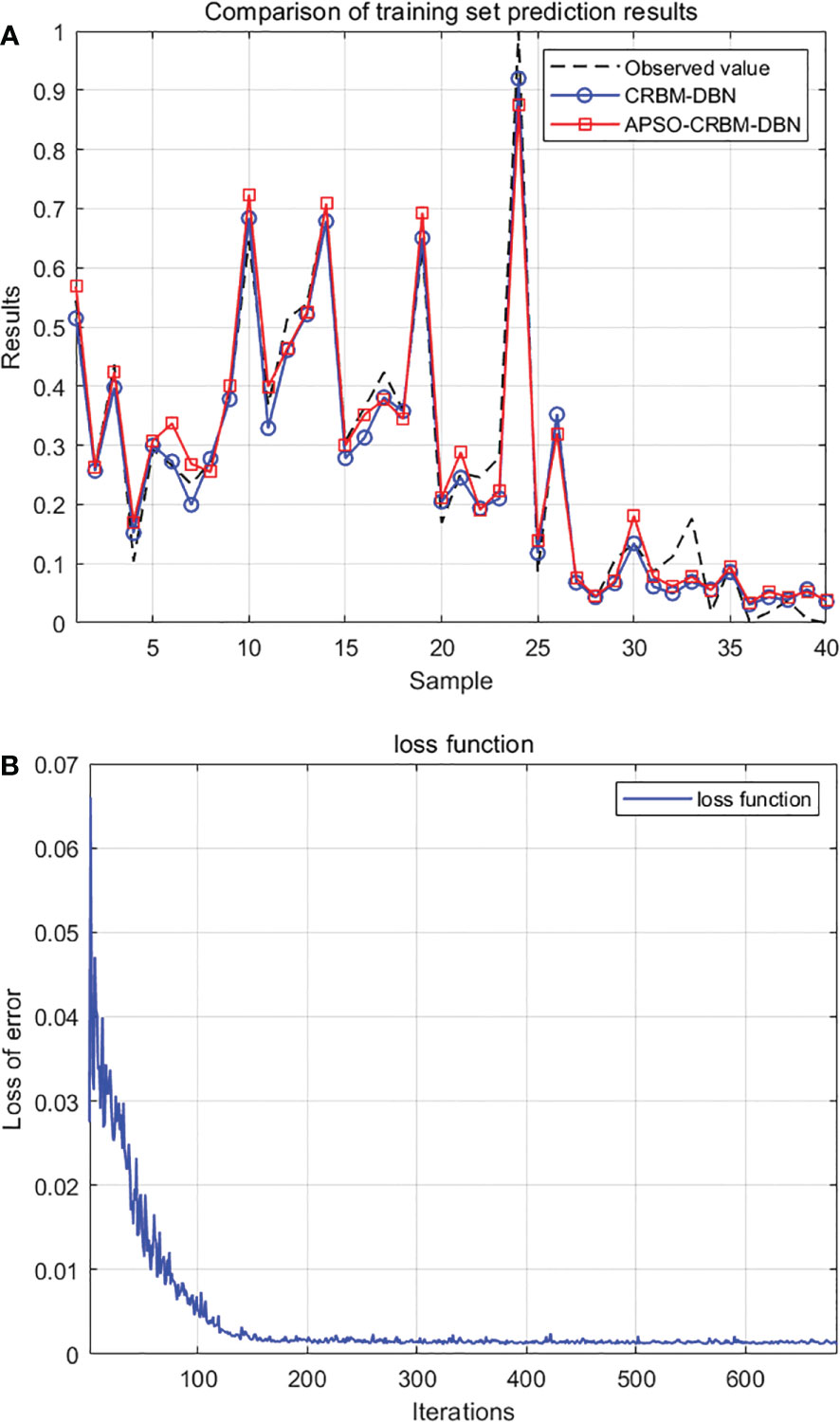
Figure 4 Model prediction results. (A) Comparison before and after optimization. (B) Predict model error losses.

4 Conclusion

Based on the real-time monitoring data of the Binhai Nuclear Power Plant, this paper carried out research on the prediction method of disaster-causing biomass of nuclear power plants. The main input environmental parameters were selected by parameter correlation analysis, and the deep learning algorithm of particle swarm optimization was adopted to simulate the nonlinear relationship between marine environmental parameters and typical disaster-causing organisms, taking the tip pen cap snails as an example. The model suitable for nuclear power cold source disaster-induced biomass prediction is trained, and the effectiveness of the model is effectively verified by performance indicators, which has important practical significance for solving the problem of biological blockage of cold source water intakes in nuclear power plants.

Data availability statement

The original contributions presented in the study are included in the article/Supplementary Material. Further inquiries can be directed to the corresponding author.

Author contributions

JH and SL designed the model. CL, LY, and JL collected and analyzed the data. YS completed the model test. JH and LS finished the algorithm program writing. JH completed writing the paper. All authors contributed to the article and approved the submitted version.

Funding

This work was supported by the open Research Fund of the Key Laboratory of Marine Ecological Monitoring and Restoration Technology, Ministry of Natural Resources [MEMRT202116], the Innovation Fund of the National Center for Marine Technology [Y1200Z006], and the Key R&D Plan of China [2018YFC1407506].

Acknowledgments

The author wishes to thank senior engineer SL, senior engineer CL, engineer LS, engineer LY, and senior engineer YS for their helpful comments to improve this paper.

Conflict of interest

Author Lei Sun is employed by Toec Technology Co., Ltd, Tianjin, China.

The remaining authors declare that the research was conducted in the absence of any commercial or financial relationships that could be construed as a potential conflict of interest.

Publisher’s note

All claims expressed in this article are solely those of the authors and do not necessarily represent those of their affiliated organizations, or those of the publisher, the editors and the reviewers. Any product that may be evaluated in this article, or claim that may be made by its manufacturer, is not guaranteed or endorsed by the publisher.

Supplementary material

The Supplementary Material for this article can be found online at: https://www.frontiersin.org/articles/10.3389/fmars.2023.1100396/full#supplementary-material

References

French G., Mackiewicz M., Fisher M., Challiss M., Knight P., Robinson B., et al. (2019). “JellyMonitor: Automated detection of jellyfish in sonar images using neural networks,” in 2018 14th IEEE International Conference on Signal Processing (ICSP). (Beijing, China: IEEE) 406–412. doi: 10.1109/ICSP.2018.8652268

CrossRef Full Text | Google Scholar

Han Y., Chang Q., Ding S., Gao M., Zhang B., Li, et al. (2022). Research on multiple jellyfish classification and detection based on deep learning. Multimedia Tools Appl. 14), 81. doi: 10.1007/s11042-021-11307-y

CrossRef Full Text | Google Scholar

Kim H., Koo J., Kim D., Jung S., Shin J. U., Lee S., et al. (2016). Image-based monitoring of jellyfish using deep learning architecture. IEEE Sensors J. 16 (8), 2215–2216. doi: 10.1109/JSEN.2016.2517823

CrossRef Full Text | Google Scholar

Kim K., Myung H. (2018). Autoencoder-combined generative adversarial networks for synthetic image data generation and detection of jellyfish swarm. IEEE Access, 6, 54207–54214. doi: 10.1109/ACCESS.2018.2872025

CrossRef Full Text | Google Scholar

Martin-Abadal M., Ruiz-Frau A., Hinz H., Gonzalez-Cid Y. (2020). Jellytoring: real-time jellyfish monitoring based on deep learning object detection. Sensors (Basel, Switzerland) 20 (6), 1708. doi: 10.3390/s20061708

PubMed Abstract | CrossRef Full Text | Google Scholar

Meng Y. H., Liu L., Guo X. J., Liu N., Liu Y. (2018). An early-warning and decision-support system of marine organisms in a water cooling system in a nuclear power plant. J. Dalian Ocean Univ. 33 (01), 108–112. doi: 10.16535/j.cnki.dlhyxb.2018.01.017

CrossRef Full Text | Google Scholar

Meng W., Liu Y., Jian-Wen L. I., Liu X. L., Guo X. J., Cheng Z. J. (2019). Early warning model for marine organism detection in a nuclear power plant based on multi-source information fusion technology. Journal of Dalian Ocean University 34, 06, 840–845. doi: 10.16535/j.cnki.dlhyxb.2019-020

CrossRef Full Text | Google Scholar

Meng W., Liu Y., Zong H., Liu X., Meng Y., Li ,. J. (2018). “Early warning model for marine organism detection in nuclear power stations,” in 2018 Chinese control and decision conference (CCDC), (Shenyang, China: IEEE) 1999–2004. doi: 10.1109/CCDC.2018.8407454

CrossRef Full Text | Google Scholar

Ruan G. (2015). Reason analysis and corresponding strategy for cooling water intake blockage at nuclear power plants. nuclear power engineering. Nuclear Power Engineer. 36(S1), 151–154. doi: 10.13832/j.jnpe.2015.S1.0151

CrossRef Full Text | Google Scholar

Tang Z., Cheng F., Jin X., Sun L., Bao R., Liu Y., et al. (2017). An automatic marine-organism monitoring system for the intake water of the nuclear power plant. Ann. Nucl. Energy. 109, 208–211. doi: 10.1016/j.anucene.2017.05.040

CrossRef Full Text | Google Scholar

Yang L., Zong H., Wei M. (2018). “Early warning model for marine organism detection based on BP neural network,” in 2018 37th Chinese Control Conference (CCC). (Wuhan, China: IEEE) 1909–1914. doi: 10.23919/ChiCC.2018.8483112

CrossRef Full Text | Google Scholar

Zhang J., Zhang S., An C., Luan Y., Li W. (2020). An effective detection method based on the biological acoustic characteristics of the outlet of nuclear power plant. IOP Conf. Ser. Mater. Sci. Eng. 780, 22034. doi: 10.1088/1757-899X/780/2/022034

CrossRef Full Text | Google Scholar

Zohdi E., Abbaspour M. (2019). Harmful algal blooms (red tide): A review of causes, impacts and approaches to monitoring and prediction. Int. J. Environ. Sci. Technol. 16 (3), 1789–1806. doi: 10.1007/513762-018-2108-X

CrossRef Full Text | Google Scholar