The strategies preventing particle transportation into the inlets of nuclear power plants: Mechanisms of physical oceanography

The formation of aquatic organism aggregations near the inlets of nuclear power plants (NPPs) has become an important global concern, as the aggregated organisms can block the cooling systems of NPPs, and, therefore, threaten their operational safety. In this study we focus on the trajectory of aquatic organisms, that is., how these organisms can be transported to the inlets of NPPs by physical ocean processes related to currents and waves. The Changjiang NPP, located on the west side of Hainan Island in China, is occasionally subject to serious gulfweed blocking events in spring. To study the physical mechanism, with the use of a three-dimensional numerical current–wave-coupled model, the current and wave conditions near the NPP were simulated. Based on the model, several particle-tracking simulations were run to evaluate the extent of the blocking that occurred in the inlet of the NPP’s cooling system with different forcings introduced. The results showed that the windage effect and the surface Stokes drift induced by waves were the main causes of blocking events in the Changjiang NPP, with the former transporting surface particles from upstream and the latter transporting surrounding particles onshore, into the NPP’s inlet. Further simulations revealed that bending of the inlet and changing the offshore mouth to downstream mouth could limit the blocking greatly, as particles were seldom transported into the mouth by cross-shore transport processes such as the Stokes drift. We suggest that such findings may provide a valuable reference for the development of strategies to prevent aquatic organism aggregation events in other NPPs.

1 Introduction

With the intensive studies and applications of nuclear power, more and more nuclear power plants (NPPs) are being built around the globe. When it comes to the maintenance and management of NPPs, the problem of blockages in NPP cooling systems is particularly serious, because of the high risk it poses to the operational safety of NPPs. The primary cause of NPP blocking events is the formation of aquatic organism aggregations. The rate of growth and aggregation of aquatic organisms is closely bound up with their surrounding environment, and this relationship has been a focus for many researchers (e.g., Li et al., 2011; Zeng et al., 2021; Liu et al., 2022). However, physical ocean processes, such as the tide, ocean circulation, and waves, can also cause blocking events by transporting organisms into the inlets of NPPs, and research into these processes is scarce.

Despite the vertical mixing associated with wind and turbulence, aquatic organisms stay afloat on the ocean surface most of the time owing to their inherent buoyancy and comparatively weak swimming ability, meaning that the surface current has a critical role in the transportation of these organisms. Depending on the dominant forcings, and space or timescales, currents can be divided into different components, including geostrophic currents, and tides and density-driven flows. Surface currents are dominated by wind and wave dynamics, which means that the Ekman current and the Stokes drift are critical to surface particle transport. The Ekman current (Ekman, 1905) is induced by winds; it is strong at the surface and decays with depth. The direction of the Ekman current deviates from the wind direction at a relative angle that changes with depth and shallow topography, being right and left of the wind at surface level in the northern and southern hemispheres, respectively. The Stokes drift (Stokes, 1847) is a material transport mechanism arising from the depth-varying orbital velocities of Stokes’s wave motions. The Stokes drift occurs at a much thinner layer than the Ekman current, but it can nevertheless significantly contribute to the surface transport of aquatic organisms: the current magnitude over the upper few centimeters of the water column can be several-fold greater than the average over the upper 10 m (Tamura et al., 2012; Clarke and van Gorder, 2018; Laxague et al., 2018). In open oceans, where waves are mostly generated by local winds, the Stokes drift direction and magnitude are closely related to wind conditions. Meanwhile, in nearshore regions, where waves are generally swell waves that have propagated from afar, the Stokes drift direction changes with water depth. This process is called wave refraction, and can be explained by Snell’s law. It results from the decrease in wave phase velocity that occurs in response to reduced water depth as the wave propagates onshore. The wave changes direction, following the direction of the gradient of water depth, leading to the onshore Stokes drift transport. The estimation of the Stokes drift from observational data has been the focus of many articles (e.g., Ardhuin et al., 2009; Ardhuin et al., 2018), in which the wind-dependent proxy approximations, or the more precise calculations using wave spectra, have been used to estimate the Stokes drift. The latter is commonly used as the parameterization in numerical models with different modifications (e.g., Breivik et al., 2014; Breivik et al., 2016).

The use of numerical models is quite practical in studying the trajectory and transport mechanism of surface particles, as it requires fewer human and material resources. The challenges of applying numerical models lies in the accuracy of simulating particle trajectories, which in turn depends on the model resolution as well as the correct expressions of the introduced forcings. Current models calculate current fields by solving the continuity and Navier–Stokes momentum equations; however, the validity of model results is constrained over a certain scale because of limitations related to their computational cost and Courant–Friedrichs–Lewy (CFL) conditions; in other words, such models cannot reproduce real physical processes, such as waves and turbulence, on a small scale. Meanwhile, the generation, propagation, and dissipation of waves are simulated using either phase-resolving or phase-averaged models. Phase-resolving models describe the actual wave motion in great detail, with a resolution that is within the scale of wavelength and wave period, but are seldom used in studies to investigate particle tracking as their computational cost is too high, and they are generally useful only in a laboratory setting, in which detailed analysis is conducted. Phase-averaged models, however, focus on the conservation of wave energy, and are therefore the preferred choice in wave modeling (Holthuijsen, 2007).

The combined use of current and wave models provides us with more accurate data for the calculation of particle trajectories. However, currents and waves are not independent from each other. The theory underlying wave–current interaction (WCI) has been studied and debated in many articles (e.g., McWilliams et al., 2004; Lane et al., 2007; Ardhuin et al., 2008; Mellor, 2008; Bennis et al., 2011). WCI can be divided into two parts: current effects on waves (CEW) and wave effects on currents (WEC). CEW, in most studies, is introduced as the Doppler shifts by currents and elevation changes in the wave dispersion relation; while WEC is a bit more complicated, and includes conservative terms such as wave-induced pressure, material transport by the Stokes drift, and vortex force, as well as non-conservative terms related to wave breaking and bottom drag. In model applications, the inclusion of WEC shows indirect impacts on the current field, especially in the nearshore region, where the wave-breaking processes are intensive (Uchiyama et al., 2009; Uchiyama et al., 2010; Guérin et al., 2018); such impacts are the result of energy transfer and dissipation induced by waves, which link to the physical processes such as the Stokes drift, wave breaking, wave spreading, white bubbles, surface roughness shifting, etc. (Cavaleri et al., 2012; Suzuki and Fox-Kemper, 2016).

Current-wave-coupled models have been adopted in many studies to explore the role of surface current and waves in the transport of floating particles, such as oil, algae, and microplastics (e.g., Drivdal et al., 2014; Fraser et al., 2018; Onink et al., 2019). For example, Fraser et al. (2018) found that kelp could travel over 20,000 km and cross the strong circumpolar currents to reach Antarctica by ocean eddies and the Stokes drift; Onink et al. (2019) found that the accumulation of floating microplastic particles was mainly due to Ekman currents, while the Stokes drift could lead to increased transport to Arctic regions.

Apart from current and wave, windage effect and turbulence movement also play a role in surface particle transport. The term “windage effect” or “leeway” describes the direct forcing effect of wind, pushing surface particles; it is not only dependent on local wind conditions, but it is also associated with the size, shape, and exposed area of particles (Chubarenko et al., 2016). Such inherence makes it difficult to replicate the windage effect in particle-tracking simulations, as particles have different characteristics, and even a change in the area exposed may change the transport trajectory. To date, the windage effect has most commonly been expressed in particle-tracking simulations as a simplified term, which is proportional to the local wind speed (e.g., Breivik et al., 2011; Duhec et al., 2015). Turbulence movement takes place at such a small scale that it is hard to reproduce it accurately in current models; it is highly random, but could be important to particle transport related to the mixing process (Steinbuck et al., 2011; Grimes et al., 2021). In particle-tracking simulations, turbulence movement is usually parameterized as a random walk term associated with the local diffusivity.

In this paper, we describe the use of a current–wave-coupled model to study the trajectory of aquatic organisms near the Changjiang NPP, which is located on the west side of Hainan Island in China, and occasionally experiences blocking events in spring, when gulfweed outbreaks occur in the nearby area. The goal of this paper is to explore the physical mechanisms that transport gulfweed into the inlet of the NPP, and discuss strategies that could help to prevent subsequent blocking events.

2 Methodology

2.1 Study region

We chose the Changjiang NPP and its surrounding area as our study region (Figure 1A). There are two sites where gulfweed outbreaks commonly occur, about 3 km and 5 km east of the NPP along the coast (Figure 1B). At these sites, large quantities of gulfweed are seen frequently on the ocean surface, particularly in spring, as the gulfweed’s rotten roots detach from the ocean floor, causing gulfweed to float upwards. As a result of currents and winds shifting in a southwestward direction during weather events, gulfweed from these two sites comes to be in the NPP’s upstream area, and sometimes causes blocking events inside the NPP’s inlet. In early November 2021, a small field campaign was carried out in our study region, with four acoustic Doppler current profilers (ADCPs) deployed at different stations (Figure 1A) to collect current data for 3 days; these data were used for current validation to assess the model performance. Unfortunately, there was a lack of observational station data for waves in our study region. As an alternative, L3-significant wave height data from Jason-3 (NOAA/EUMETSAT/NASA/CNES), SARAL/AltiKa (CNES/ISRO) and CFOSAT (CNSA/CNRS/IFREMER/SHOM/METEOFRANCE) satellites were used to evaluate the wave field calculated by model over the entire model domain (Figure 1C).

FIGURE 1

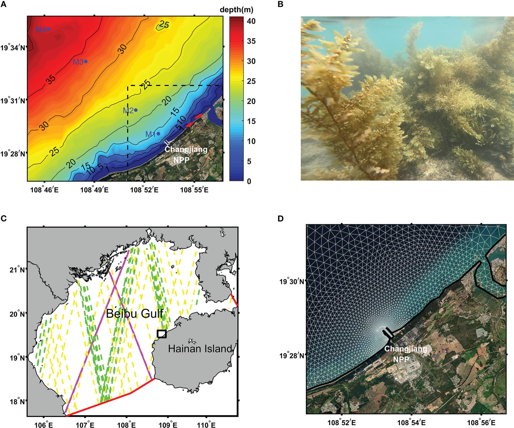
Figure 1 (A) The study region with bottom topography (colored shading). The positions of current stations are indicated by blue markers. The two red elliptical markers indicate the locations of two gulfweed source sites near the coast. The dashed rectangular box marks the area of particle release in particle-tracking simulations, whereas the solid white line at the coast outlines the inlet mouth of the Changjiang nuclear power plant (NPP). (B) Photograph of gulfweed taken at the source locations. The gulfweed plants in the photograph are approximately 2 m in height. (C) Model domain. The two solid red lines are the open boundaries of the model. Dashed lines track the Jason-3 (magenta), SARAL/AltiKa (yellow), and CFOSAT (green) satellite trajectories from late December 2018 to early April 2019. The solid black rectangular box corresponds to the study region. (D) Computational grid in the study region (white line). Note that this is only part of the model grid. The entire grid over the model domain is not shown.

2.2 Model description and setting

The semi-implicit cross-scale hydroscience integrated system model (SCHISM) was used to calculate current fields in our study. SCHISM is a three-dimensional (3D), unstructured-grid ocean model that solves the Reynolds-averaged Navier–Stokes equation using the semi-implicit finite-element formulation, which shows enhanced numerical stability and low numerical dissipation (Zhang et al., 2016). The high flexibility of SCHISM makes it appropriate for model applications of cross-scale interactions as well as ocean regions with complex topography and coastlines. As an open source, community-supported model, SCHISM has been adopted worldwide, and it is continually being developed by the embedding of different modules into its model system, such as those for waves, sediment transport, and ecosystem. The wave module embedded in SCHISM is based on the third-generation spectral wind–wave model (WWM) of Roland et al. (2012), which is a phase-averaged model that calculates wave fields by solving the wave action equation (e.g., Komen et al., 1994) as follows:

$\begin{array}{ll}\frac{\partial }{\partial t}N + {\nabla }_X(\dot{X}N) + \frac{\partial }{\partial \sigma }(\dot{\sigma }N) + \frac{\partial }{\partial \theta }(\dot{\theta }N) = S_{tot},& (1)\end{array}$

where ∇_X is the horizontal gradient operator, σ is the relative wave frequency, and θ is the wave direction; $\dot{X}$, $\dot{\sigma }$, and $\dot{\theta }$ are the velocities in the geographical, frequency, and direction phase spaces, respectively; N denotes to E/σ, with E being the variance density of surface elevations; and S_tot is the total source term, including energy input from wind and non-linear wave interactions, as well as energy dissipation by whitecapping, wave breaking, and bottom friction. The coupling of SCHISM and WWM is conducted at a source code level by exchanging variables between the two models with the same subdomains in the parallel MPI implementation to ensure efficiency and avoid interpolation. During the exchange, values for water elevation, wet and dry flags, and velocities are passed from SCHISM to WWM to calculate CEW, while the calculated radiation stress or vortex force term, total surface stress, and wave orbital velocity (needed for the calculation of wave-induced bottom stress) from WWM are run through SCHISM to determine WEC.

The entire computational grid we used covered a larger domain (Figure 1C) that included our study region (Figure 1D), with the horizontal spatial resolution ranging from about 3 km in the central area to approximately 30 m at the land boundary. There was a sink being set at the inner side of the Changjiang NPP’s inlet, with a constant sucking flux of 100 m³/s. The discretization of 23 layers in the vertical direction was adopted based on the hybrid S–Z coordinates, with h_c , θ_b , and θ_f set to 10, 0.7, and 5.0, respectively. The model simulation period was from 1 November 2018 to 10 April 2019, and the SCHISM model was run twice—one run was coupled with WWM, whereas the other was not, so that wave effect could be explored from the comparably different outcomes. In early November 2021, an additional run was carried out to compare the model performance with the observational current data from the field campaign. SCHISM and WWM shared the same computational grid and the same time step of 60 s. The boundary data of SCHISM were obtained using a robust operational ocean model simulation of the Taiwan Strait (Liao et al., 2013; Chen et al., 2014; Lin et al., 2016), which provided daily temperature, salinity, and velocity measurements for the linear interpolation at the open boundary. Tidal forcing was calculated from 13 main tidal constituents obtained from the FES2014 tide model (Carrere et al., 2016). The atmospheric data, with a 1-hour time resolution and 0.2° spatial resolution from the weather research and forecast (WRF) model product of the Fujian Marine Forecasts, were used to compute atmospheric forcing in SCHISM and WWM. The five necessary wave parameters (significant wave height, mean wave direction, mean directional spreading, peak frequency, and mean zero-downcrossing wave period) for constructing wave spectra at the open boundary were interpolated using the data from a global hindcast product (Rascle and Ardhuin, 2013). The vortex force formulation was chosen for the coupling in WWM with the wave roller turned off, and both spectral and direction discretization were set to 30 bins. The initial fields for SCHISM were obtained from the same ocean model product for boundary data, whereas the initial fields for WWM were set to zero since the wave field developed quickly enough to remove initial error within hours.

2.3 Particle-tracking simulations

A Lagrangian particle‐tracking model is provided inside the SCHISM code package for post processing of the model outputs. In our study cases, we assumed that the gulfweed keeps floating at the ocean surface, and thus only the horizontal movement of particles was calculated. Such assumptions are valid, as gulfweed is buoyant and does not have the ability to move vertically in the way, for example, that dinoflagellate does. When adopting all the forcing terms, the trajectory of each gulfweed particle is calculated independently according to the below formula:

$\begin{array}{ll}\Delta X = (U + W + \nabla K_X + SD)\Delta t + RW,& (2)\end{array}$

where ΔX is the horizontal position change for each time step, and Δt is the time step interval; U is the water velocity and W is the proxy of windage effect, which is set to 3% of local wind speed at a 10-m height in our study; ∇K_X is horizontal gradient of diffusion coefficient, which is used to calculate the virtual advection term from regions of low to high diffusivity to prevent spurious aggregation (Visser, 1997); SD is the overall surface Stokes drift; and RW is the random walk representing turbulence movement. The SD term is calculated from WWM by summing the surface Stokes drift of each spectral and direction bin with:

$\begin{array}{ll}{U}_{st} = \sigma \overrightarrow{\mathit{\text{k}}}\frac{\text{cosh}(2kz + 2kD)}{{\text{sinh}}^2(kD)}E,& (3)\end{array}$

where σ and E are the same as in Equation (1), $\overrightarrow{\mathit{\text{k}}}$ is the horizontal wavenumber vector, D is the water depth, and z equals zero at the surface. Finally, the RW term is calculated with a smaller time step by $R\sqrt{6K_X(\Delta t^{*})}$, with R being a uniform random number between –1 and 1, K_X being the turbulent diffusion coefficient, and Δt^* being half of the time step. By alternately adding or removing the W, SD, and RW terms in Equation (2), the corresponding simulation results can be compared to investigate the impacts of windage effect, the Stokes drift, and turbulence movement, respectively.

All the simulations were carried out from 1 to 5 April 2019, as a serious gulfweed blocking event occurred during this period. Particle trajectories were calculated using the outputs at 10-min interval from SCHISM (and WWM in the case of the coupled run). For each model output, the particle positions were upgraded in 100 substeps using Equation (2). By carrying out sensitivity experiments, we found that the variation in results decreased as the number of substeps increased, and at the number of substeps we adopted, 100, approximated to zero. During each simulation, particles were released every hour throughout the first simulation day; thereafter, the simulation was kept running for the last 4 simulation days without any particles being released. In each release, 1,452 particles were placed uniformly on the ocean surface at approximately 200-m intervals throughout the study region (Figure 1A), with the exception of the coastal area, where water depth was less than 0.5 m, to reduce unnecessary computational costs. As a result, each particle release site had 24 trajectories, corresponding to the 24 release times, in the first simulation day for each particle-tracking simulation; the probabilistic intensity of each spot was calculated as the ratio of the number of trajectories that came to be inside the NPP’s inlet to the total number (which is exactly 24) of trajectories.

3 Results

3.1 Model validation

Figure 2 shows the current validation results between the 3-day observational station data and the corresponding model outputs in November 2021, which included eastward velocity and northward velocity at three depths: near surface, middle layer, and near bottom. The basic statistics—mean bias (MB), root-mean-square difference (RMSD), and correlation coefficient (CC)—are shown in Table 1. In general, the calculated currents at stations agreed well with observations, with correlation coefficients higher than 0.8 in some station layers. Orbital significant wave heights from atellite data and model outputs over the whole model domain from late December 2018 to early April 2019 are compared in Figure 3, which reveals an overall good model performance for waves, with MB, RMSD, and CC being 0.11 m, 0.41 m, and 0.84, respectively.

FIGURE 2

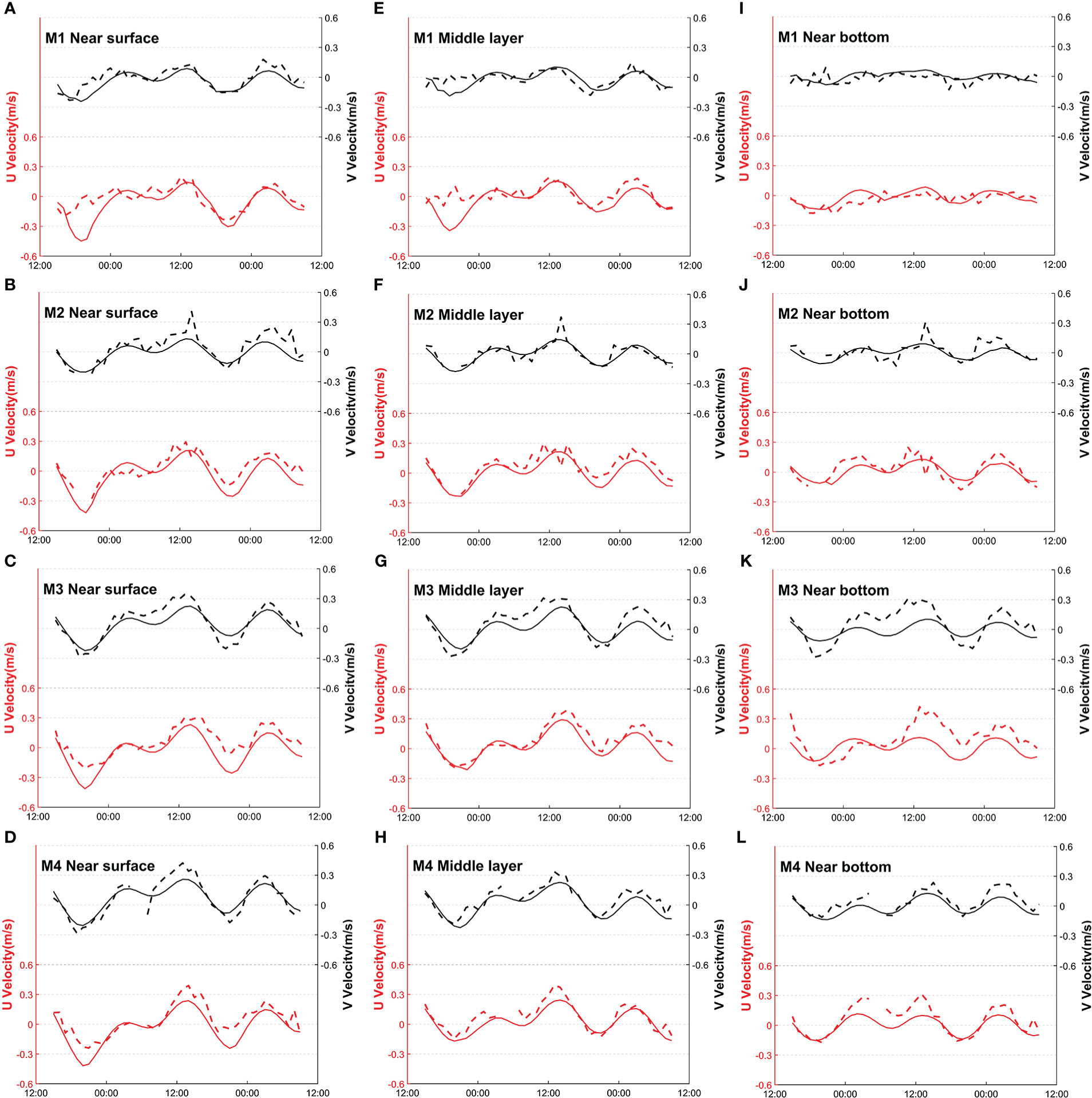
Figure 2 (A–L) Current validation between observational data and model outputs at the near surface, middle layer, and near bottom of M1, M2, M3, and M4 stations operating from 2 to 4 November 2021. The black lines at the top indicate northward current velocity (V) at different times (right-hand axis), whereas the red lines below indicate eastward current (U) velocity (left-hand axis). Dashed lines are observational data, and solid lines are model outputs.

TABLE 1

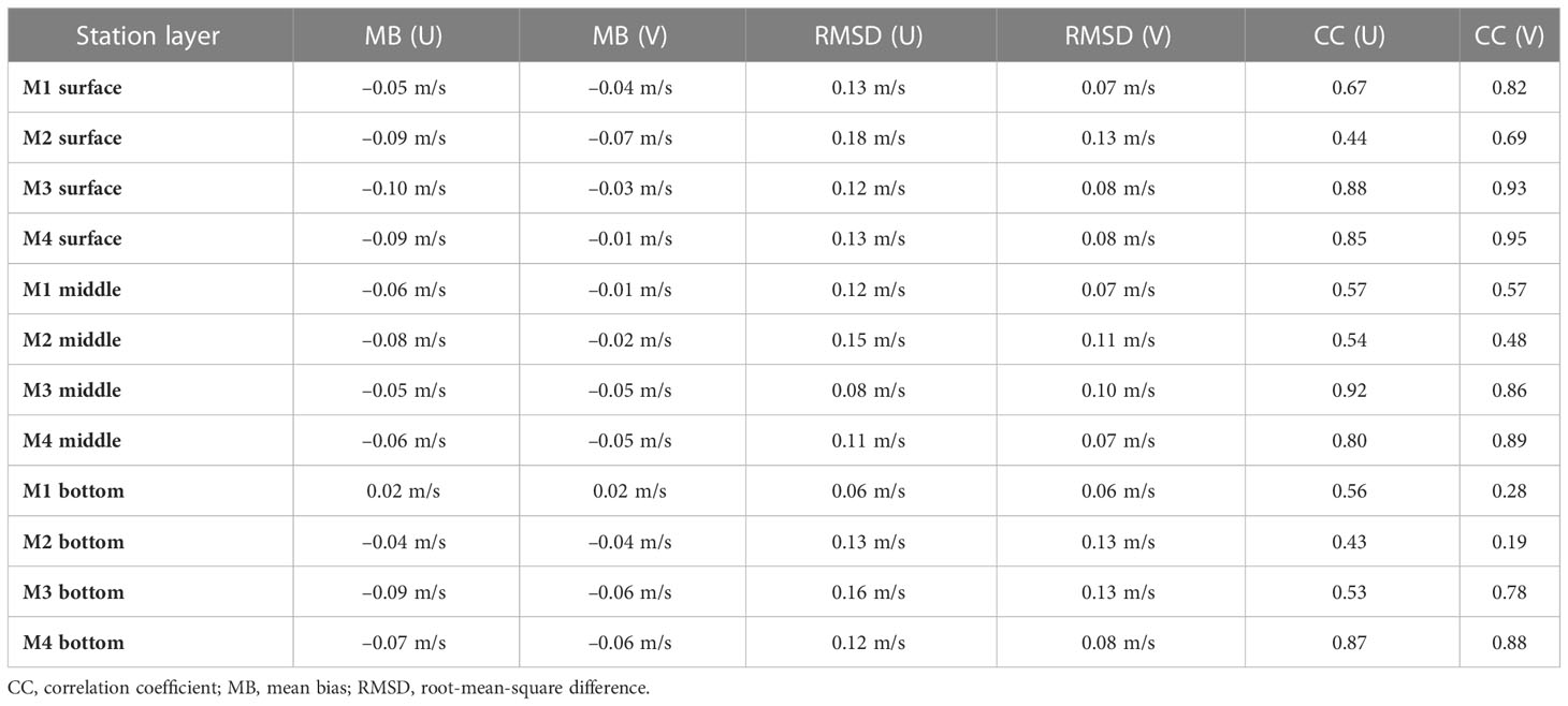
Table 1 Basic statistics for current validation between observational data and model outputs.

FIGURE 3

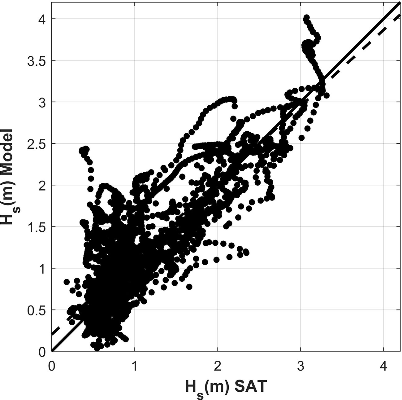
Figure 3 Scatter diagram of significant wave height from the satellite data and corresponding model outputs. The solid black line indicates the ideal fit and the black dashed line shows the linear regression for the two datasets, with a slope of 0.92.

3.2 Current, wind, and the Stokes drift fields

Figure 4 shows the time-averaged fields in the study region during the simulation period (1–5 April 2019). The mean surface current field (Figure 4A) reveals that there is a general southwestward velocity higher than 0.1 m/s in the region, with the magnitude dropping near the shore and the current direction slightly shifting toward the west in offshore areas. The wind field at a 10-m height (Figure 4B) showed a nearly homogeneous pattern, with the direction being southwestward over the region, and the magnitude dropping linearly from north to south. As for the surface Stokes drift field (Figure 4C), its direction was more southward than that for the current and wind field offshore, and became perpendicular to the coast as it got near the shore. The Stokes drift velocity was at its highest near the shore, and was at its lowest close to the coastline and inside the NPP’s inlet.

FIGURE 4

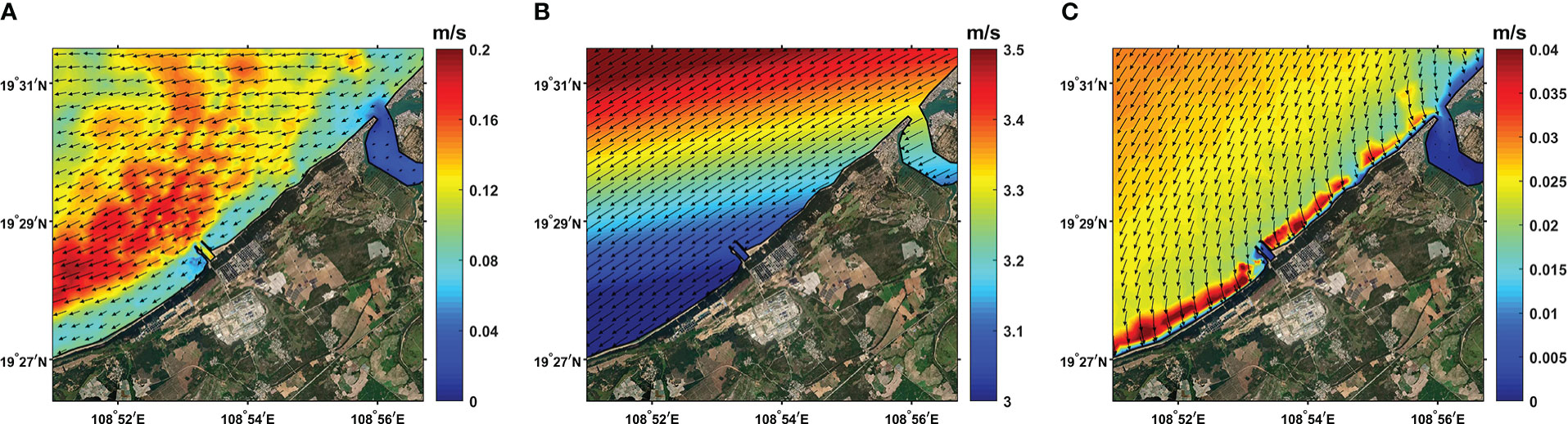
Figure 4 Time-averaged horizontal fields during the simulation period (1–5 April 2019), with colored shading showing the vector magnitude. (A) Surface current field. (B) Wind field at a 10-m height. (C) The surface Stokes drift field.

3.3 Particle-tracking simulation results

The results of the probabilistic intensity (hereinafter PI) distributions of the different simulations are shown in Figure 5, and the setting for each simulation can be found in Table 2. PI indicates the relevance of the location of released particles to their likelihood of reaching the NPP’s inlet. A PI of 100% indicates that all of the particles released in a given location will be transported to the NPP’s inlet during the simulation period, whereas a PI of 0% indicates that all of the released particles at a given location will not be transported to the NPP’s inlet. For each simulation, a non-zero PI value occurred only at the area upstream of the inlet, near the coast, which indicated that this area accounted for the particle transport into the inlet. When the windage effect was included (Figures 5D–F), the area with a high PI value extended upstream along the coast from the inlet to the outside of the study region, covering the two gulfweed source sites. The pattern of the highest PI value in the simulation was seen when the Stokes drift was included (Figure 5F), with the area with a PI value exceeding 90% occurring approximately 6 km upstream from the inlet and about 500 m offshore. The simulation results of the current model without waves (Figure 5D) showed a slightly different pattern, that is, a high PI value applied to the area at a shorter distance off the coast, but a low PI value extended further offshore. The simulation results of the current–wave model without the Stokes drift included resulted in an area with a high PI value that was smaller than in the case of the other two simulations (Figure 5E), as the area to which a low PI value applied was further offshore than in the simulation including the Stokes drift (Figure 5F), but covered a shorter distance than the simulation without waves (Figure 5D). With the windage effect excluded (Figures 5A–C, the PI distributions of the three simulation results showed obvious shrinking compared with those with the windage effect included (Figures 5D–F), with a high PI value observed only in the area very close to the east side of the inlet and pressed into the coastline as it extended upstream, and no longer covering the two gulfweed source sites. The simulation of current–wave model with the Stokes drift had the highest PI value among the three simulations (Figure 5C), with the area to which its non-zero PI value applied extending about 10 km upstream from the inlet. The impact of turbulence movement on particle trajectories in our study, whether or not included, was negligible in all simulations (not shown in this paper).

FIGURE 5

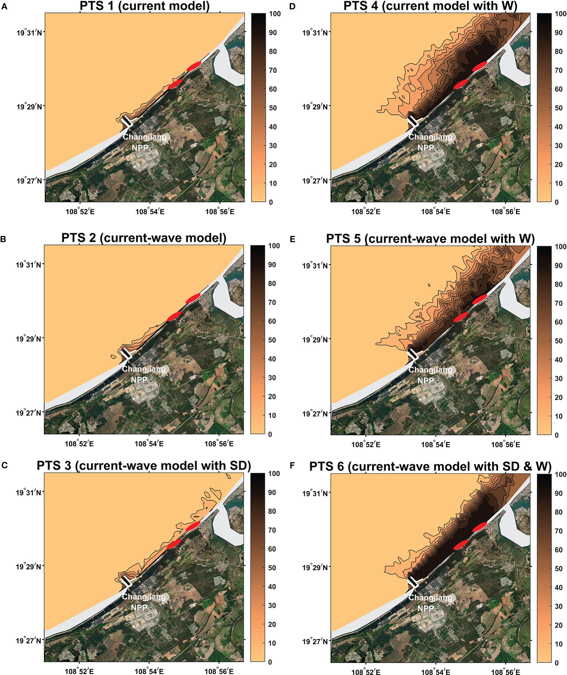
Figure 5 (A–F) Probabilistic intensity distributions of different particle-tracking simulation results. Color shading represents the odds (expressed as a percentage) of the particles released in the region being transported into the NPP’s inlet. The higher the value, the greater the likelihood that particles released at that location are transported into the inlet during the simulation period. The two red elliptical markers indicate the locations of two gulfweed sources near the coast.

TABLE 2

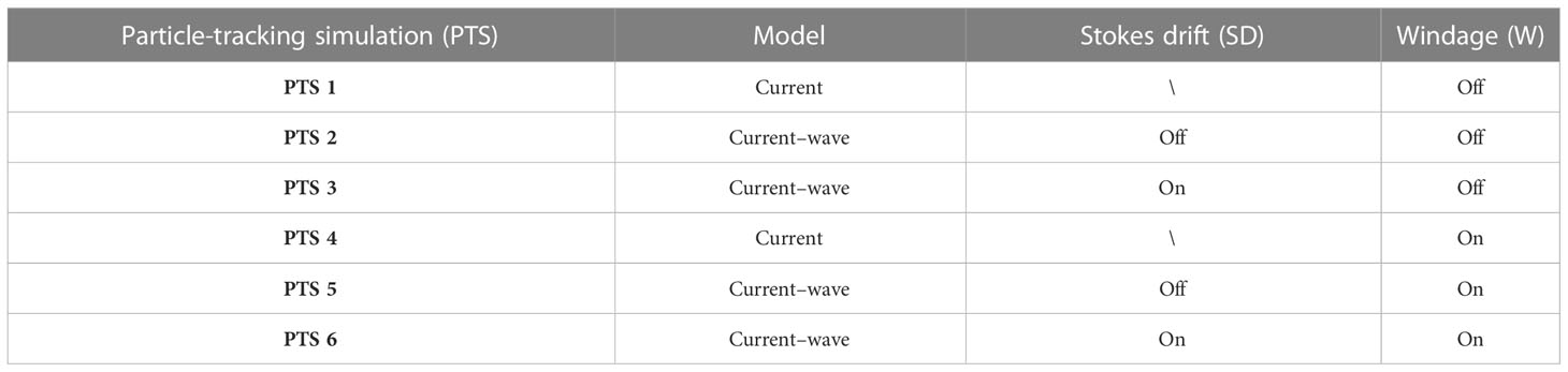
Table 2 Experimental settings for particle-tracking simulations.

4 Discussion

The formation of aquatic organism aggregations can lead to blocking events in NPP inlets, and thus compromise the operational safety of NPPs. In addition to the local growth and aggregation related to environmental disturbances, the transport of aquatic organisms can also be the cause of blocking events. To study the physical processes associated with currents and waves that transport aquatic organisms into the inlets of NPPs, a 3D current–wave-coupled model with high resolution was used to provide current and wave fields for the post-processed particle-tracking simulations (computational resolution should be of a higher standard when wave fields are to be calculated in a numerical model, as wave at the ocean surface is mainly related to wind speed, which in turn has a time period in seconds). With a spatial resolution of 30 m near the coast and a time step of 60 s for solving both currents and waves, the coupled model we used was sufficient to simulate the physical processes of interest for this study. The validation results revealed good model performance, though we used the satellite data to validate modeled wave fields only because of the lack of observational station data for waves in our study region.

Particle-tracking simulations compute the trajectory of virtual particles with the introduced forcings. In this paper, we used the field data of current, wave, and wind provided by model to simulate the gulfweed trajectory, as gulfweeds transported from the nearby area could cause serious blocking events inside the inlet of the NPP in our study region. With probabilistic intensity (PI) calculated from the simulation results, we evaluated the impact of different forcings on the gulfweed transport that could lead to blocking inside the NPP inlet.

Before looking at the simulation results, the time-averaged fields (Figure 4) during the simulation period partly revealed the role of current, wind, and the Stokes drift induced by wave action. The surface current (Figure 4A) transported upstream particles near the coast with an increased velocity magnitude, as well as a slightly offshore inclination, which would move particles away from the inlet as they floated downstream. Meanwhile, wind moving in a southwestward direction (Figure 4B), and the associated decrease in velocity magnitude along its direction, would be more likely to cause the accumulation of particles in the downstream area. Finally, the surface Stokes drift showed an onshore velocity overall (Figure 4C). Near the shore, the Stokes drift reached its maximum velocity while its direction became more perpendicular to the coast, which in turn caused strong cross-shore transport of particles. These field patterns showed that current, wind, and the Stokes drift have different impacts on the transport of particles in different areas. For example, although the current had a higher order of magnitude than the Stokes drift over the study region, the inverse could be true near the shore, where the current is weak and the Stokes drift is strong.

The windage effect is an important forcing in particle-tracking simulations, for it represents the direct wind forcing on surface particles. We used a 3% wind speed at a 10-m height as a proxy for the windage effect to simplify evaluation of its impact on particle tracking. The simulation results showed that the PI value in the upstream area of the inlet increased greatly when the windage effect was introduced (Figures 5D–F), and in most areas, the PI value exceeded 60%, compared with its value of less than 20% without the inclusion of the windage effect (Figures 5A–C). The fact that high PI values at the two gulfweed source sites were observed only when windage effect was included indicates that the windage effect was the main force that transported gulfweed from the gulfweed source sites to the NPP’s inlet. Simulations carried out in late December 2018 produced similar results (not shown in this paper). All of these simulation results revealed that windage effect had a significant part in the blocking events in our study region. In fact, cross-shore transport only counts when particles are transported by windage effect from an upstream area to the surrounding of the inlet mouth.

For model calculations, the windage effect, along with the Stokes drift, is generally estimated as being 3% of local wind speed at a 10-m height. However, such rough estimations are clearly not applicable to all scenarios. Haza et al. (2019) evaluated different parameterizations of Lagrangian velocity in the northern Gulf of Mexico using substantial trajectories of the drifters launched during the Lagrangian submesoscale experiment (LASER). The authors found variations in trajectory improvement under different wind and wave conditions, as well as in different geographic regions. As our model adopted only the wind-dependent estimation of the windage effect, without considering other factors, further studies are needed to provide a more comprehensive view.

The highest PI value was observed in the simulation that included both the Stokes drift and the windage effect (Figure 5F), and revealed the significance of the Stokes drift to the transportation of particles to the NPP’s inlet in our study region. Because of wave refraction, the Stokes drift shifted in a direction more perpendicular to the coast as it got closer to shore. As a result, stronger cross-shore transport occurred near the shore when the Stokes drift force was included in the simulation, which led in turn to more opportunities for the upstream particles to be transported into the offshore inlet mouth. In addition, this could account for the serious blocking events inside the inlet.

Apart from the Stokes drift, the wave effect could also indirectly have an impact on the current (WEC). Near the shore region, WEC mainly changes the current pattern by two processes: the offshore anti-Stokes flow and the littoral wave-induced current. The anti-Stokes flow results from the onshore Stokes drift, that is, to maintain the water conservation, the onshore Stokes drift would cause an anti-flow to balance the water transport. Guérin et al. (2018) studied the effect of WEC on water setup near the coast and found a typical wave-induced vertical circulation—an onshore flow at the upper layer and an offshore undertow, the magnitude of which changes with the beach slope and wave energy. The study of littoral wave-induced current can be traced back to the works of Longuet-Higgins (1970a, 1970b), which found that the littoral current was the result of the dynamic balance between bottom friction and an introduced wave dissipation term. Uchiyama et al. (2009) found that a strong littoral current occurred at the location where wave breaking was strong, with the bottom drag adjusting the current—broad, weak current with low drag, and narrow, strong current with high drag. From our results, the WEC can be seen in Figures 5D and E—when the Stokes drift transport was excluded from the particle-tracking simulations, the current–wave-coupled model (Figure 5E) indicated that the chance of the particles being transported into the NPP’s inlet was, overall, lower than that in the current model without waves (Figure 5D), which might be related to the offshore transport of the anti-Stokes flow, as well as to the strong littoral wave-induced current.

To support the discussions of the transport forcing terms mentioned above, another model simulation was run to provide additional analysis results. The model and post-processed particle-tracking simulations were run using the same settings as the original ones, except for the model computational grid, which used a downstream mouth of the inlet (C2, Figure 6A) instead of the original offshore mouth structure (C1, Figure 1D). The results showed that the PI distributions were the same pattern for all simulations (Figure 6B)—non-zero PI values were observed only inside the inlet, which revealed an absolute isolation of the inlet for the outside surface particles. These results support our theory that cross-shore means of particle transportation, such as the Stokes drift, have an important impact on blocking events, as it was shown that, when adopting a downstream structure for the NPP inlet, blocking events could be greatly limited through the prevention of the cross-shore transportation of particles from upstream.

FIGURE 6

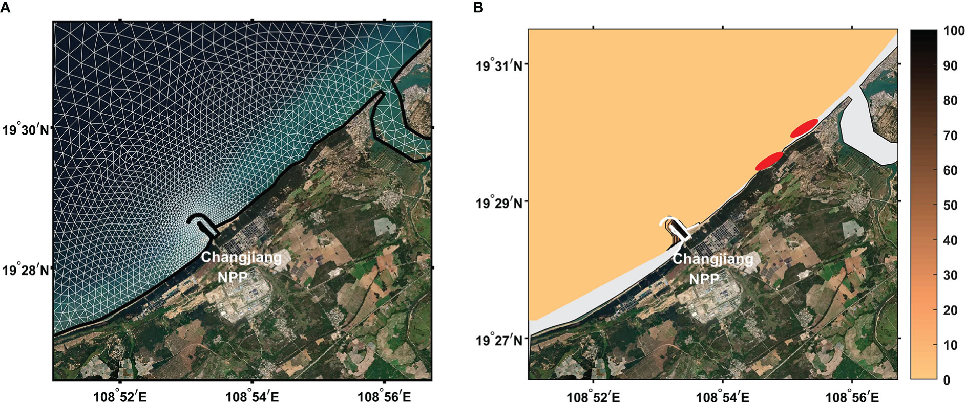
Figure 6 (A) Computational grid in the study region (white line) for the new model case. (B) Probabilistic intensity distribution calculated from outputs of the new model case, which yields the same result for all particle-tracking simulations. The two red elliptical markers indicate the locations of two gulfweed source sites near the coast.

The current–velocity profiles of the two model cases were compared. The profile sections selected for the two cases are shown in Figure 7, with two magenta dots marking the section fragment closest to the inlet mouth. In each case, four velocity profiles at 6-hour intervals were chosen to analyze the current pattern, with a positive value (red) representing inflow to the inlet and a negative value (blue) representing outflow from the inlet (Figure 8). The current profiles of C1 (offshore mouth) showed a relatively stable pattern, with an inflow velocity core maintaining at the middle layer (Figures 8A–D), which reflected the constant sucking flux of the NPP’s inlet. The surface current was mostly inflow, and it had a magnitude of approximately 0.02 m/s, which was comparable to those of the surface current and the Stokes drift around the inlet mouth (Figure 7A). In addition, both the surface current and the Stokes drift transported particles into the inlet. Meanwhile, for C2 (downstream mouth), the current profiles were more unstable and without an obvious pattern, which could have strong velocity shear vertically (Figures 8E, F) or horizontally (Figures 8G, H with surface outflow and underneath inflow). The mechanism of such pattern shifts might be due to the interaction between topography and tidal activity in the region, which requires further exploration, and is currently out with the scope of our study. Nevertheless, we did observe that the high current variation, along with the negligible surface Stokes drift near the downstream mouth (Figure 7B), added more uncertainty to particle trajectories, which might account for their reduced inlet-blocking opportunities when compared with C1.

FIGURE 7

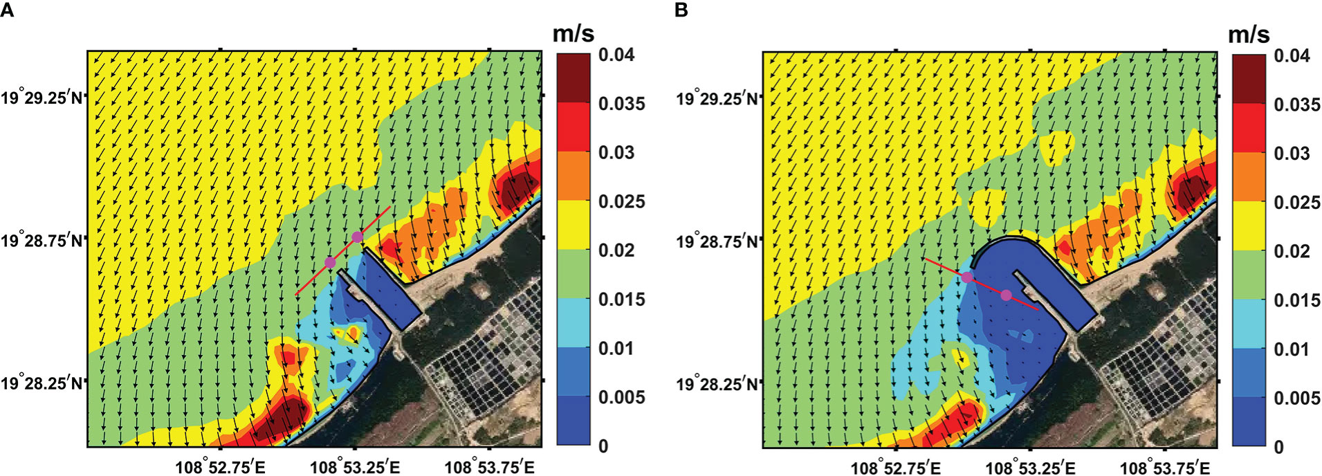
Figure 7 The position of current–velocity profile section (red line) for two model cases: (A) C1, with an offshore inlet mouth, and (B) C2, with a downstream inlet mouth. The two magenta dots in the red line mark the section fragment closest to the inlet mouth. The black vectors indicate the mean surface Stokes drift on 2 April 2019, with color shading representing the vector magnitude.

FIGURE 8

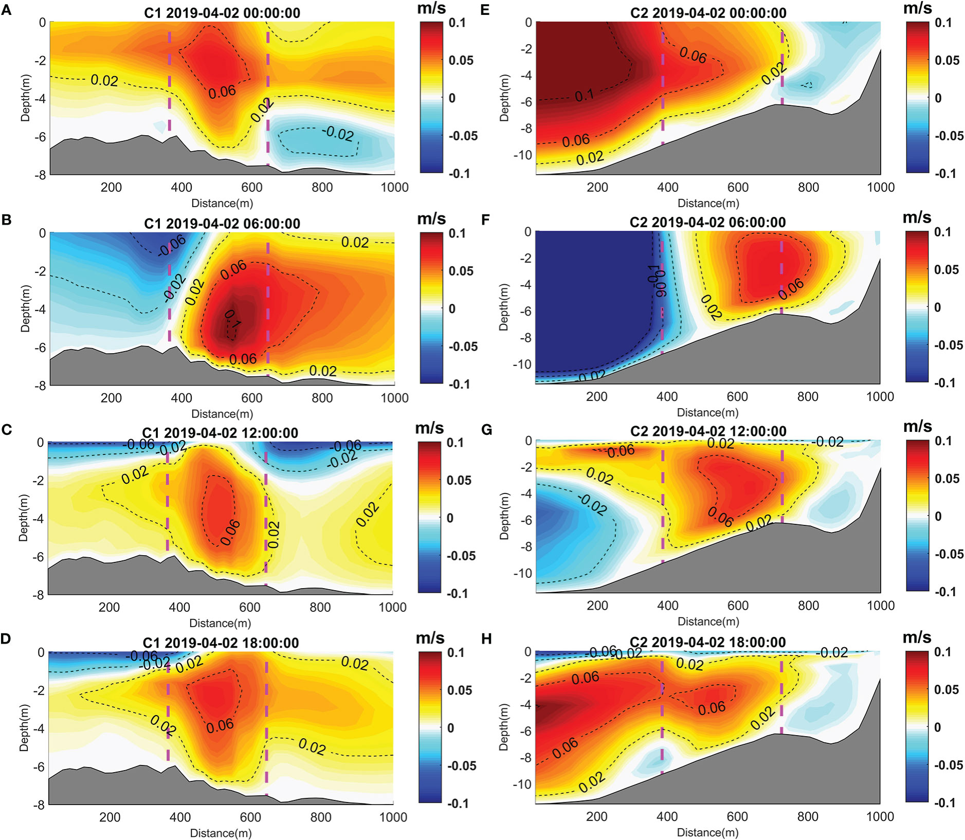
Figure 8 Velocity profiles with 6-hour intervals of the two model cases: (A–D) C1, with an offshore inlet mouth, and (E–H) C2, with a downstream inlet mouth. Colored shading represents the horizontal velocity magnitude perpendicular to the section, with a positive value (red) representing inflow and a negative value (blue) representing outflow near the inlet. The gray patch is the section topography, whereas the two magenta vertical lines correspond to the two magenta dots in Figure 7, which mark the section fragment closest to the inlet mouth.

In conclusion, our results suggested that windage effect and the Stokes drift had an important impact on gulfweed blocking events inside the NPP’s inlet in our study. With the wind field being appropriate, that is, the two gulfweed sources being upstream of the NPP, the windage effect would transport gulfweed from the gulfweed source sites to the inlet’s surroundings, and the Stokes drift would then transport surrounding gulfweed onshore into the inlet. Further simulations revealed that a downstream mouth structure of the inlet could greatly limit the likelihood of blocking by interrupting the cross-shore transport from the Stokes drift, which might be a potential prevention strategy for blocking events in other NPPs. However, there are some aspects of the research in this paper which are open to improvement and further exploration. For example, the proxy for the windage effect could be improved by considering particle characteristics, as well as considering adjustments under different conditions; the results of different wave model setting should be compared with the study of the role of wave action in dissipation processes, such as wave breaking and wave-induced bottom drag; and the physical mechanism responsible for the current pattern near the inlet requires further dynamic diagnosis.

Data availability statement

The raw data supporting the conclusions of this article will be made available by the authors, without undue reservation.

Author contributions

JLi and MX performed the research and prepared the manuscript. JLin provided necessary support for conducting the field campaign. YJ supervised the work, and provided supportive data and guidance for numerical models. All authors contributed to the article and approved the submitted version.

Acknowledgments

This work was supported by the Chinese Ministry of Science and Technology through the National Key Research and Development Program of China (2022YFA1004404). The field work was supported by grant (U22A20579, 41961144011, 41876004) from Natural Science Foundation of China (NSFC). S. Fang, Y. Yu and Z. Xu from Information and Network Center of Xiamen University are acknowledged for the help with the high-performance computing.

Conflict of interest

The authors declare that the research was conducted in the absence of any commercial or financial relationships that could be construed as a potential conflict of interest.

Publisher’s note

All claims expressed in this article are solely those of the authors and do not necessarily represent those of their affiliated organizations, or those of the publisher, the editors and the reviewers. Any product that may be evaluated in this article, or claim that may be made by its manufacturer, is not guaranteed or endorsed by the publisher.

References

Ardhuin F., Aksenov Y., Benetazzo A., Bertino L., Brandt P., Caubet E., et al. (2018). Measuring currents, ice drift, and waves from space: the sea surface kinematics multiscale monitoring (SKIM) concept. Ocean Sci. 14, 337–354. doi: 10.5194/os-14-337-2018

CrossRef Full Text | Google Scholar

Ardhuin F., Jenkins A. D., Belibassakis K. A. (2008). Comments on ‘‘The three-dimensional current and surface wave equations’’. J. Phys. Oceanography 38, 1340–1350. doi: 10.1175/2007JPO3670.1

CrossRef Full Text | Google Scholar

Ardhuin F., Marie L., Rascle N., Forget P., Roland A. (2009). Observation and estimation of lagrangion, stokes, and eulerian currents induced by wind and waves at the sea surface. J. Phys. Oceanography 39, 2820–2838. doi: 10.1175/2009JPO4169.1

CrossRef Full Text | Google Scholar

Bennis A. C., Ardhuin F., Dumas F. (2011). On the coupling of wave and three-dimensional circulation models: choice of theoretical framework, practical implementation and adiabatic tests. Ocean Model. 40, 260–272. doi: 10.1016/j.ocemod.2011.09.003

CrossRef Full Text | Google Scholar

Breivik Ø., Allen A., Maisondieu C., Roth J. (2011). Wind-induced drift of objects at sea: the leeway field method. Appl. Ocean Res. 33, 100–109. doi: 10.1016/j.apor.2011.01.005

CrossRef Full Text | Google Scholar

Breivik Ø., Bidlot J. R., Janssen P. A. (2016). A stokes drift approximation based on the Phillips spectrum. Ocean Model. 100, 49–56. doi: 10.1016/j.ocemod.2016.01.005

CrossRef Full Text | Google Scholar

Breivik Ø., Janssen P. A., Bidlot J. R. (2014). Approximate stokes drift profiles in deep water. J. Phys. Oceanography 44, 2433–2445. doi: 10.1175/JPO-D-14-0020.1

CrossRef Full Text | Google Scholar

Carrere L., Lyard F., Cancet M., Guillot A., Picot N. (2016). FES 2014, a new tidal model–validation results and perspectives for improvements. ESA Living Planet Conference Prague.

Google Scholar

Cavaleri L., Fox-Kemper B., Hemer M. (2012). Wind waves in the coupled climate system. Bull. Am. Meteorological Soc. 93, 1651–1661. doi: 10.1175/BAMS-D-11-00170.1

CrossRef Full Text | Google Scholar

Chen Z. Y., Yan X. H., Jiang Y. W. (2014). Coastal cape and canyon effects on wind-driven upwelling in northern Taiwan strait. J. Geophysical Res. Oceans 119, 4605–4625. doi: 10.1002/2014jc009831

CrossRef Full Text | Google Scholar

Chubarenko I., Bagaev A., Zobkov M., Esiukova E. (2016). On some physical and dynamical properties of microplastic particles in marine environment. Mar. pollut. Bull. 108, 105–112. doi: 10.1016/j.marpolbul.2016.04.048

PubMed Abstract | CrossRef Full Text | Google Scholar

Clarke A., van Gorder S. (2018). The relationship of near-surface flow, stokes drift, and the wind stress. J. Geophysical Res. Oceans 123, 4680–4692. doi: 10.1029/2018JC014102

CrossRef Full Text | Google Scholar

Drivdal M., Broström G., Christensen K. H. (2014). Wave-induced mixing and transport of buoyant particles: application to the statfjord a oil spill. Ocean Sci. 10, 977–991. doi: 10.5194/os-10-977-2014

CrossRef Full Text | Google Scholar

Duhec A. V., Jeanne R. F., Maximenko N., Hafner J. (2015). Composition and potential origin of marine debris stranded in the western Indian ocean on remote Alphonse island, Seychelles. Mar. pollut. Bull. 96, 76–86. doi: 10.1016/j.marpolbul.2015.05.042

PubMed Abstract | CrossRef Full Text | Google Scholar

Ekman V. W. (1905). On the influence of the earth’s rotation on ocean currents. Arch. Math. Astron. Phys. 2, 1–52.

Google Scholar

Fraser C. I., Morrison A. K., Hogg A. M., Macaya E. C., van Sebille E., Ryan P. G., et al. (2018). Antarctica’s ecological isolation will be broken by storm-driven dispersal and warming. Nat. Climate Change 8, 704–708. doi: 10.1038/s41558-018-0209-7

CrossRef Full Text | Google Scholar

Grimes D. J., Feddersen F., Giddings S. N. (2021). Long-Distance/Time surf-zone tracer evolution affected by inner-shelf tracer retention and recirculation. J. Geophysical Res. Oceans 126, 1–22. doi: 10.1029/2021jc017661

CrossRef Full Text | Google Scholar

Guérin T., Bertin X., Coulombier T., de Bakker A. (2018). Impacts of wave-induced circulation in the surf zone on wave setup. Ocean Model. 123, 86–97. doi: 10.1016/j.ocemod.2018.01.006

CrossRef Full Text | Google Scholar

Haza A. C., Paldor N., Özgökmen T. M., Curcic M., Chen S. S., Jacobs G.. (2019). Wind-based estimations of ocean surface currents from massive clusters of drifters in the gulf of Mexico. J. Geophysical Research: Oceans 124, 5844–5869. doi: 10.1029/2018jc014813

CrossRef Full Text | Google Scholar

Holthuijsen L. H. (2007). Waves in oceanic and coastal waters (Cambridge, U. K: Cambridge University Press), 1–7.

Google Scholar

Komen G. J., Cavaleri L., Donelan M., Hasselmann K., Hasselmann S., Janssenet P. A. (1994). Dynamics and modelling of ocean waves (Cambridge, U. K: Cambridge University Press), 532.

Google Scholar

Lane E. M., Restrepo J. M., McWilliams J. C. (2007). Wave–current interaction: A comparison of radiation-stress and vortex-force representations. J. Phys. Oceanography 37, 1122–1141. doi: 10.1175/JPO3043.1

CrossRef Full Text | Google Scholar

Laxague N. J. M., Özgökmen T. M., Haus B. K. (2018). Observations of near-surface current shear help describe oceanic oil and plastic transport. Geophysical Res. Lett. 45, 245–249. doi: 10.1002/2017gl075891

CrossRef Full Text | Google Scholar

Liao E. H., Jiang Y. W., Li L., Hong H. S., Yan X. H. (2013). The cause of the 2008 cold disaster in the Taiwan strait. Ocean Model. 62, 1–10. doi: 10.1016/j.ocemod.2012.11.004

CrossRef Full Text | Google Scholar

Li T., Liu S., Huang L., Huang H., Lian J., Yan Y., et al. (2011). Diatom to dinoflagellate shift in the summer phytoplankton community in a bay impacted by nuclear power plant thermal effluent. Mar. Ecol. Prog. Ser. 424, 75–85. doi: 10.3354/meps08974

CrossRef Full Text | Google Scholar

Lin X. Y., Yan X. H., Jiang Y. W., Zhang Z. C. (2016). Performance assessment for an operational ocean model of the Taiwan strait. Ocean Model. 102, 27–44. doi: 10.1016/j.ocemod.2016.04.006

CrossRef Full Text | Google Scholar

Liu Q., Zhou L., Zhang W., Zhang L., Tan Y., Han T., et al. (2022). Rising temperature contributed to the outbreak of a macrozooplankton creseis acicula by enhancing its feeding and assimilation for algal food nearby the coastal daya bay nuclear power plant. Ecotoxicology Environ. Saf. 238. doi: 10.1016/j.ecoenv.2022.113606

CrossRef Full Text | Google Scholar

Longuet-Higgins M. S. (1970b). Longshore currents generated by obliquely incident sea waves: 2. J. Geophysical Res. 75, 6790–6801. doi: 10.1029/JC075i033p06790

CrossRef Full Text | Google Scholar

Longuet-Higgins M. S. (1970a). Longshore currents generated by obliquely incident sea waves: 1. J. Geophysical Res. 75, 6778–6789. doi: 10.1029/JC075i033p06778

CrossRef Full Text | Google Scholar

McWilliams J. C., Restrepo J. M., Lane. E. M. (2004). An asymptotic theory for the interaction of waves and currents in coastal waters. J. Fluid Mechanics 511, 135–178. doi: 10.1017/S0022112004009358

CrossRef Full Text | Google Scholar

Mellor G. L. (2008). The depth-dependent current and wave interaction equations: a revision. J. Phys. Oceanography 38, 2587–2596. doi: 10.1175/2008JPO3971.1

CrossRef Full Text | Google Scholar

Onink V., Wichmann D., Delandmeter P., van Sebille E. (2019). The role of ekman currents, geostrophy, and stokes drift in the accumulation of floating microplastic. J. Geophysical Research: Oceans 124, 1474–1490. doi: 10.1029/2018JC014547

CrossRef Full Text | Google Scholar

Rascle N., Ardhuin F. (2013). A global wave parameter database for geophysical applications. part 2: Model validation with improved source term parameterization. Ocean Model. 70, 174–188. doi: 10.1016/j.ocemod.2012.12.001

CrossRef Full Text | Google Scholar

Roland A., Zhang Y. J., Wang H. V., Meng Y., Teng Y., Maderich V., et al. (2012). A fully coupled 3D wave-current interaction model on unstructured grids. J. Geophysical Research: Oceans 117, C00J33. doi: 10.1029/2012jc007952

CrossRef Full Text | Google Scholar

Steinbuck J. V., Koseff J. R., Genin A., Stacey M. T., Monismith S. G. (2011). Horizontal dispersion of ocean tracers in internal wave shear. J. Geophysical Res. 116, C11031. doi: 10.1029/2011JC007213

CrossRef Full Text | Google Scholar

Stokes G. G. (1847). On the theory of oscillatory waves. Trans. Cambridge Philos. Soc. 8, 441–473.

Google Scholar

Suzuki N., Fox-Kemper B. (2016). Understanding stokes forces in the wave-averaged equations. J. Geophysical Research: Oceans 121, 3579–3596. doi: 10.1002/2015JC011566

CrossRef Full Text | Google Scholar

Tamura H., Miyazawa Y., Oey L.-Y. (2012). The stokes drift and wave-induced mass flux in the north pacific. J. Geophysical Res. 117, C08021. doi: 10.1029/2012JC008113

CrossRef Full Text | Google Scholar

Uchiyama Y., McWilliams J. C., Restrepo J. M. (2009). Wave-current interaction in nearshore shear instability analyzed with a vortex force formalism. J. Geophysical Res. 114, C06021. doi: 10.1029/2008jc005135

CrossRef Full Text | Google Scholar

Uchiyama Y., McWilliams J. C., Shchepetkin A. F. (2010). Wave–current interaction in an oceanic circulation model with a vortex-force formalism: Application to the surf zone. Ocean Model. 34, 16–35. doi: 10.1016/j.ocemod.2010.04.002

CrossRef Full Text | Google Scholar

Visser A. W. (1997). Using random walk models to simulate the vertical distribution of particles in a turbulent water column. Mar. Ecol. Prog. Ser. 158, 275–281. doi: 10.3354/meps158275

CrossRef Full Text | Google Scholar

Zeng L., Chen G., Wang T., Zhang S., Dai M., Yu J., et al. (2021). Acoustic study on the outbreak of creseise acicula nearby the daya bay nuclear power plant base during the summer of 2020. M Mar. pollut. Bull. 165. doi: 10.1016/j.marpolbul.2021.112144

CrossRef Full Text | Google Scholar

Zhang Y. J., Ye F., Stanev E. V., Grashorn S. (2016). Seamless cross-scale modeling with SCHISM. Ocean Model. 102, 64–81. doi: 10.1016/j.ocemod.2016.05.002

CrossRef Full Text | Google Scholar